On compatibility of string effective action with an accelerating universe

Abstract

In this paper, we fully investigate the cosmological effects of the moduli-dependent one-loop corrections to the gravitational couplings of the string effective action to explain the cosmic acceleration problem in early (and/or late) universe. These corrections comprise a Gauss-Bonnet (GB) invariant multiplied by universal non-trivial functions of the common modulus $\sigma$ and the dilaton $\phi$. The model exhibits several features of cosmological interest, including the transition between deceleration and acceleration phases. By considering some phenomenologically motivated ansatzs for one of the scalars and/or the scale factor (of the universe), we also construct a number of interesting inflationary potentials. In all examples under consideration, we find that the model leads only to a standard inflation ($w\geq-1$) when the numerical coefficient $\delta$ associated with modulus-GB coupling is positive, while the model can lead also to a non-standard inflation ($w<-1$), if $\delta$ is negative. In the absence of (or trivial) coupling between the GB term and the scalars, there is no crossing between the $w<-1$ and $w>-1$ phases, while this is possible with non-trivial GB couplings, even for constant dilaton phase of the standard picture. Within our model, after a sufficient amount of e-folds of expansion, the rolling of both fields $\phi$ and $\sigma$ can be small. In turn, any possible violation of equivalence principle or deviations from the standard general relativity may be small enough to easily satisfy all astrophysical and cosmological constraints.

1 Introduction

Dark energy, or cosmological vacuum energy, spread on every point in space exerts gravitationally smooth and negative pressure and hence leads to cosmic inflation, a phenomenon which is not accounted for by ordinary matter and General Relativity (GR). Unfortunately, at the moment the origin of dark energy (and its associated cosmic acceleration) is arguably the murkiest question in cosmology - and the one that, when answered, may provide deepest insights into the origin (and the fate) of our universe, establishing synergies between the microscopic physics and cosmological length scales.

In recent years, the cosmic acceleration problem has been addressed in hundreds of papers proposing various kinds of modification of the energy-momentum tensor in the ‘vacuum’ – the source of gravitationally repulsive negative pressure. Some examples of recent interest include braneworld modifications of Einstein’s GR [1], scalar-tensor gravity [2], phantom (ghost) field [3], K-essence [4] or ghost condensate [5], $f(R)$-gravity that adds terms proportional to inverse powers of $R$ [6] or $R^{n}$ ($n\geq 2$) terms, or both these effects at once [7], thereby modifying in a very radical manner the Einstein’s GR itself. All these proposals typically include a more or less disguised feature, non-locality, other than classical or quantum instabilities. A recent review by Copeland, Sami and Tsujikawa [8] summarizes the prospects and limitations of these proposals in an elegant way.

String theory is much more ambitious and far reaching than any of the above ideas, and it may be compatible with a de Sitter universe (see, e.g. [9]). It has been known that a cosmological compactification of classical supergravity – the low energy description of string/M theory – on compact hyperbolic spaces [10, 11], or Ricci-flat twisted spaces [12], naturally leads to a period of cosmic acceleration. Furthermore, fundamental scalar fields abundant in such higher–dimensional gravity theories potentially provide a natural source for gravitationally repulsive vacua, as well as a mechanism for generating the observed density perturbations [13]. In this respect, the best framework where one can hope to fully explain the dark energy effect is perhaps string/M theory.

A strong motivation for a cosmology based on string theory [14], that goes beyond the standard cosmology and incorporates Einstein’s theory in a more general framework, is that it may shed light on the nature of the cosmological singularities arising in GR. Moreover, string theory has the prospect of unification of all other interactions, see [15] for a review. An interesting question is which version of string theory, if any, among the presently known five (which are related to each other by various dualities [16]), best describes the physical world. A successful superstring theory should naturally incorporate realistic cosmological solutions.

String theory, as a theory of quantum gravity in one time and nine space dimensions, literally contains (or predicts) an infinite number of scalar fields. Most of the scalars in string theory, arising from a compactification to four-dimensions, are structure moduli associated with the (six-dimensional) internal geometry of space (Calabi-Yau spaces or Calabi-Yau shapes), which do not directly couple with the spacetime curvature tensor and hence to Einstein gravity [17]. It is well appreciated that, at least, one of the Kähler moduli (or the modulus associated with the overall size of the internal compactification manifold) naturally couples to (standard) Einstein gravity via Riemann curvature invariants [18, 19].

According to conventional wisdom superstrings involve a minimum length scale only a few order of magnitude larger than the Planck length, $l_{P}\sim{10}^{-33}$ cm, and, in turn, string theory leads to a modification of Einstein’s theory only at very short distances. This idea is perfectly reasonable when we study small fluctuations in the fixed (time-independent) background, but may not be generally true, for the scalars such as the dilaton ($\phi$) and the modulus field ($\sigma$) and their couplings to various curvature terms, which arise universally in any four-dimensional heterotic superstring model, may be important in any cosmological solution of the string effective action (see, for example [20, 21]). In this paper, we therefore investigate as to whether the evolutions of $\phi$ and $\sigma$, and their couplings to a Gauss-Bonnet term, can explain the cosmic acceleration problem at early (and/or late) universe.

This paper is organized as follows. In section 2 we briefly discuss the limitations of a standard cosmological model where Einstein’s gravity is coupled to a scalar field with a self-interaction potential alone. In section 3 we first motivate ourselves to a more general action which consists of, in addition to a standard scalar potential, scalars dependent loop corrections to the gravitational couplings of the string effective action and write the full set of field equations for the metric, the modulus and the dilaton. In section 4 we first write down the equations of motion as a monotonous system of first order differential equations, and present various analytic solutions by allowing at most two variables of the model to take some specific forms. In section 5, we do a similar analysis but expressing the field equations in an alternative form, which we find more appropriate for implementing our knowledge about the coupling functions and the behaviour of the accelerating solutions at early or late-times. At the end of both sections 4 and 5 we provide an overview of the different solutions being discussed there. In section 6, we will have a cursory look in the system where gravity is non-minimally coupled to mater and radiation. Our conclusions are summarized in section 7.

2 The standard scenario

In a standard cosmological scenario, one assumes that for a given scalar field $\sigma$ with a self-interaction potential $V(\sigma)$, the Einstein gravity is described by the action:

$$S=\int d^{4}{x}\left[\sqrt{-g}\left(\frac{1}{2\kappa^{2}}R-\frac{\gamma}{2}(\nabla\sigma)^{2}-V(\sigma)\right)\right],$$ (1)

where $\kappa$ is the inverse Planck mass $m_{\rm Pl}^{-1}=(8\pi G_{N})^{1/2}$, $\gamma$ is the coupling constant and $\sigma$ is the classical scalar field whose stress-energy tensor is set by the choice of the potential. What one normally wants is a well motivated potential for the desired evolution. This often refers to a cosmological potential that allows at least an epoch of cosmic inflation or acceleration/deceleration regime.

A real motivation for an effective action of the form (1) arises from the fact that inflation with the dynamics of a self-interaction potential, $V(\sigma)>0$, provides a natural mechanism for generating the observed density perturbations [13]. To this end, one defines the spacetime metric in standard Friedmann-Robertson-Walker (FRW) form:

$$ds^{2}=-dt^{2}+a(t)^{2}\sum_{i=1}^{3}(dx^{i})^{2},$$ (2)

where $a(t)$ is the scale factor of the universe. The Hubble parameter that measures the expansion rate of the universe is given by $H\equiv\dot{a}/a$, where the dot denotes a derivative with respect to proper time $t$. One also assumes that the scalar field $\sigma$ obeys an equation of state (EoS), with an equation of state parameter given by

$$w\equiv\frac{p}{\rho}=-\frac{2}{3}\frac{\dot{H}}{H^{2}}-1=\frac{2q}{3}-\frac{1}{3},$$ (3)

where $q\equiv-a\ddot{a}/\dot{a}^{2}$ is the deceleration parameter. This definition of $w$ does not depend on the number of (scalar) fields in the model. The ‘equation of state’ parameter $w$ is essentially a measure of how squishy the substance is. It is when $w<-1/3$ a gravitationally repulsive pressure exerted by one or more scalar fields can drive the universe into an accelerating phase ($q<0$). In particular, the cosmological constant $\Lambda$ as a source of dark energy or vacuum energy means that $w_{\Lambda}=\rho_{\Lambda}/p_{\Lambda}=-1$.

In the last two decades, many authors have studied cosmology based on (1) by considering various ad hoc choice of the scalar potential $V(\sigma)$ (the recent reviews [22] provide an exhaustive list of references). Written in terms of the following dimensionless variables:

$${\cal X}\equiv\kappa^{2}\frac{\gamma}{2}\left(\frac{\dot{\sigma}}{H}\right)^{2},\quad{\cal Y}\equiv\kappa^{2}\frac{V(\sigma)}{H^{2}},\quad\varepsilon\equiv\frac{\dot{H}}{H^{2}},$$ (4)

the field equations, obtained by varying the action (1), satisfy the following simple relationships [23]:

$${\cal Y}=3+\varepsilon,\quad{\cal X}=-\varepsilon.$$ (5)

The time-evolution of the scalar field is given by $\sigma(t)=\kappa^{-1}\int{\rm d}{t}[-2\dot{H}/\gamma]^{1/2}$. Clearly, the model lacks its predictability, since $\varepsilon$ (and hence ${\cal Y}$) is arbitrary. This arbitrariness in the potential has motivated many physicists/cosmologists to consider models with some specific choices of the potential, e.g. quadratic/chaotic potential $V(\sigma)=V_{0}+\frac{1}{2}m^{2}\sigma^{2}$, power-law potential $V(\sigma)=\sum m_{Pl}^{4-n}\lambda_{n}\,{\sigma^{n}}$, inverse power-law potential $V(\sigma)=\Lambda^{4}(\sigma_{0}/\sigma)^{n}$ ($n\geq 2$), the axion-potential $V(\sigma)=\Lambda^{4}(C\pm\cos(\sigma/\sigma_{0}))$, etc. This approach to the problem, starting from Linde’s model of chaotic inflation [24], may be motivated from different particle physics models or effective field theory. Without a complete theory of fundamental gravity, the validity of these potentials (to explain the dark energy problem) is not clear. The choice of possibilities for the potential also mimics the fact that the exact nature and origin of an inflationary potential (or dark energy) has not been convincingly explained yet.

A common (if not conservative) argument sometimes expressed in the literature is the following. To explain a particular value of one new parameter (acceleration, i.e., the second derivative of the scale factor, $\ddot{a}$), it is enough to introduce another new parameter in the set up of the model. To this aim, one often fixes the time dependence of the scale factor, by making a particular ansätz for it, which then fixes the parameter $\varepsilon$, and then finally find a potential, using (4)-(5), which supports this particular $a(t)$. For instance, for the power-law expansion, $a(t)\propto t^{\alpha}$, such a potential is given by $V=V_{0}\,\rm e^{-\sqrt{2/\alpha}\,(\sigma/m_{\rm Pl})}$. In this fashion one may find a good approximation at each energy scale, but the corresponding solution may have little relevance when one attempts to study a wider range of scales, including an early inflationary epoch.

Action (1) is remarkably simple but not sufficiently general as it excludes, for example, the coupling between the field $\sigma$ (a run away Kähler modulus) and the Riemann curvature invariants, as predicted correctly by some version of string theory [19]. Also the best motivated scalar-tensor theories which respect most of GR’s symmetries naturally include the GB type curvature invariants multiplied by field dependent couplings. That is to say, the most general scalar-tensor theories may involve one more parameter, the GB integrand multiplied by a non-trivial function of $\sigma$ or $\phi$. One may wonder whether such extra degree of freedom added to the standard model ruins the theory, leading to a plethora of both qualitative and analytic behaviour of cosmological solutions. This is generally not the case; the knowledge about the $\sigma$ (and/or $\phi$)-dependent couplings may even help to construct a realistic cosmological model with time-varying $\varepsilon$ (which otherwise remains arbitrary) without destroying the basic characteristics of the standard model (1).

3 Effective action and equations of motion

String theory gives rise to two kinds of modifications of the Einstein’s theory. The first one is associated with the contribution of an infinite tower of massive string modes and leads to $\alpha^{\prime}$-corrections, and the second one is due to quantum loop effects (string coupling expansion) [18]. Therefore, if we wish a cosmological model to inherit maximum properties of the low energy string effective action and its associated early universe cosmology, then it may be necessary to include an additional scalar, namely, the dilaton field $\phi$, which plays the role of string loop expansion parameter. To this aim, the effective action for the system may be taken to be [19, 20]

$$S=\int d^{4}{x}\sqrt{-g}\left[\frac{1}{2\kappa^{2}}R-\frac{\gamma}{2}(\nabla\sigma)^{2}-V(\sigma)-\frac{\zeta}{2}(\nabla\phi)^{2}+\frac{1}{8}[\lambda(\phi)-\delta\xi(\sigma)]{\cal R}^{2}_{GB}\right],$$ (6)

where ${{\cal R}^{2}_{GB}}\equiv R^{2}-4R_{\mu\nu}R^{\mu\nu}+R_{\mu\nu\rho\sigma}R^{\mu\nu\rho\sigma}$ is the Gauss-Bonnet (GB) integrand. It is assumed that there is no potential term corresponding to the field $\phi$. The GB term ${\cal R}^{2}_{GB}$ has been multiplied by non-trivial functions of $\phi$ and $\sigma$, otherwise it would remain a topological invariant in four dimensions. One would expect ${\cal R}^{2}_{GB}$ to be small in the present epoch and that mass scales associated with the dilaton and the modulus to be smaller than $m_{Pl}$, so that they would not be dominating the dynamics. Only when these two conditions are met, can the higher-derivative corrections to the action be neglected and does string theory go over to an effective quantum field theory [14]. Furthermore, we will consider for most of this paper that $\gamma>0$, $\zeta>0$, so that both $\sigma$ and $\phi$ are canonical (real) scalar fields.

It is worth noting that a GB integrand multiplied by a function of $\phi$ is already present at the string tree-level in the next to leading-order $\alpha^{\prime}$ expansion [18], and a non-trivial $\xi(\sigma)$ exists at the one-loop order [19]. One also notes that the (semi)classical tests of Newtonian gravity typically deal with small fluctuations in the fixed (time-independent) background and thus are unaffected by the GB type modification of Einstein’s theory. Another beauty of the action (6) is that the equations of motion for the modulus-dilaton-graviton system form a set differential equations with no more than second derivatives of the fields or the metric, which can be solved exactly with some specific choice of the (coupling) parameters, or a prior knowledge about the evolution of one of the scalars, and/or the scale factor, $a(t)$.

As compared to the four-dimensional perturbative string effective action obtained from a compactification of 10d heterotic superstring on a symmetric orbifold [19], action (6) lacks the terms proportional to $R\tilde{R}=\eta^{\mu\nu\rho\lambda}R_{\mu\nu}\,^{\sigma\tau}R_{\rho\lambda\sigma\tau}$ (where $\eta^{\mu\nu\rho\lambda}\equiv\epsilon^{\mu\nu\rho\lambda}/\sqrt{-g}$ and $\epsilon^{\mu\nu\rho\lambda}$ a totally anti-symmetric tensor) which however give a trivial contribution in the background (2). The numerical coefficient $\delta$ typically depends on the massless spectrum of every particular model; in [19], it was found to be associated with the four-dimensional trace anomaly of the $N=2$ supersymmetry of the theory. Here we absorb this coefficient into the coupling function $\xi(\sigma)$.

An often asked question is the following: what are the choices for $V(\sigma)$, $\xi(\sigma)$ and $\lambda(\phi)$)? And what could motivate these choices? One can take a different point of view: it may be more productive to know what form of the potential (or the scalar-GB couplings) offers the best resolution to the dilemma posed by the current cosmic acceleration or the dark energy problem. In some perturbative string amplitude computations, $V(\sigma)$ appeared to be absent [19], implying that it is a phenomenologically-motivated term. Whatever the origin of the potential, $V(\sigma)$, in (6) may be, we believe that the $\sigma$-dependence of the potential is quite universal. This was also the case revealed recently from type IIB string theory compactified on a (deformed) conifold [9]; this study also includes some supersymmetry breaking non-perturbative effects, mainly those coming from different branes and fluxes present in the extra dimensions. Typically, the moduli potentials are generated by fluxes, so $V(\sigma)$ in (6) may take into account a contribution from fluxes.

Recently, [25] examined a cosmological solution for the system (6) with the simplest choice of the scalar potential and the modulus-GB coupling, namely $V(\sigma)=V_{0}{\rm e}^{-2\sigma/\sigma_{0}},\quad\xi(\sigma)=\xi_{0}{\rm e}^{2\sigma/\sigma_{0}}$, deleting the $\phi$-dependent terms. Even this simple system led to plethora of qualitative behaviors of cosmological solutions, among which one may accommodate lots of data, including the dark energy’s ‘equation of state’ parameter, $w$. However, a solution of the type $a(t)\propto t^{\alpha}$ with $\alpha>0$, or $a(t)\propto(t_{\infty}-t)^{\alpha}$ with $\alpha<0$, i.e. a power-law expansion for which $\varepsilon=$ const, does not support the transition from acceleration to deceleration as well as the crossing between quintessence ($w>-1$) to phantom ($w<-1$) phases. A non-constant $\varepsilon$ is generally required for achieving a natural exit from inflation in the early universe cosmology as well as for explaining a transition from deceleration to acceleration in the expansion of the (late) universe, which has been viewed as a recent phenomenon [26]. Thus we shall normally consider a situation in which $\varepsilon$ (and hence the EoS parameter, $w\equiv-2\varepsilon/3-1$) dynamically changes as it happens in inflationary cosmology.

A study has been recently made in [27] by considering a variant of the action (6), which includes additional $\phi$-dependent higher curvature terms and also a non-trivial coupling between $\phi$ and the Einstein-Hilbert term, i.e. in the presence of a single scalar field (a dilaton or compactification modulus). The method authors used there to find the solutions was mainly to identify analytically some asymptotic solutions and then try to join them numerically. A similar approach was taken previously in the paper [20], for the action (6) with $V(\sigma)=0$ ([28, 29] provided further generalizations with a non-zero spatial curvature). In this work, we examine the system analytically, by writing the field equations as a monotonous system of first (and second) order differential equations. In the background (2), the equations of motion derived from the action (6) are given by (see, e.g., [20, 30])

$$0=-\frac{3}{\kappa^{2}}H^{2}+\frac{\gamma}{2}\dot{\sigma}^{2}+\frac{\zeta}{2}\dot{\phi}^{2}+V(\sigma)-3H^{3}\dot{f},$$ (7)

$$0=\frac{1}{\kappa^{2}}(2\dot{H}+3H^{2})+\frac{\gamma}{2}\dot{\sigma}^{2}+\frac{\zeta}{2}\dot{\phi}^{2}-V(\sigma)+H^{2}\ddot{f}+2H\dot{H}\dot{f}+2H^{3}\dot{f},~{}~{}$$ (8)

$$0=\gamma(\ddot{\sigma}+3H\dot{\sigma})+\frac{dV(\sigma)}{d\sigma}+\frac{1}{8}\,\frac{d\xi(\sigma)}{d\sigma}\,{\cal R}^{2}_{GB},$$ (9)

$$0=\zeta(\ddot{\phi}+3H\dot{\phi})-\frac{1}{8}\,\frac{d\lambda(\phi)}{d\phi}\,{\cal R}^{2}_{GB},$$ (10)

where $f\equiv\lambda(\phi)-\xi(\sigma)$. Note that $\phi=$ const is a solution of the last equation above only if $\lambda(\phi)=$ const, implying a trivial coupling between $\phi$ and the GB term. Because of the Bianchi identity, one of the equations is redundant and may be discarded, as it will be trivially satisfied by a solution obtained by solving three equations only: equations (7) and (8) are not functionally independent. More precisely, the linear combination $H\times(7)+H\times(8)-\frac{1}{3}\,{\dot{\sigma}}\times(9)-\frac{1}{3}\,{\dot{\phi}}\times(10)$ yields the time derivative of (7). One may drop, for instance, (8), so that (7), (9) and (10) form a set of independent equations of motion.

In [23], we analysed the model by treating $\phi$ as a constant, which then leaves only $\sigma$ as a dynamical field. This analysis was partly motivated from an earlier observation by Antoniadis et al. [20], in the $V(\sigma)=0$ case, that the behaviour of solutions depends crucially on the form of $\sigma$-dependent string one-loop corrections, while the $\phi$-dependent contribution is negligible and may be ignored. This has got another clear motivation: in string theory context, fixing of the volume (or Kähler) moduli, is only an approximate idea (see, e.g.[9, 31]).

We are not interested in the situation where the contributions coming from the GB term dominates the other terms in the effective action, which is consistent with our approximation of neglecting higher derivative terms, like $(\nabla\sigma)^{4}$ and also higher curvature terms. For all solutions to be discussed below, the squared of the Hubble parameter, $H^{2}$, will decay faster than the couplings $\lambda(\phi)$ and $\xi(\sigma)$ grow with time. Thus the moduli/dilaton dependent two (and higher) loop corrections to higher derivative terms or terms higher than quadratic in the Riemann tensor, which give at least sixth powers of $H$, are small and may be neglected. Nevertheless, it is interesting to note that a four-dimensional string effective action without a Gauss-Bonnet term, but including terms up to quartic in $\sigma$, $(\nabla\sigma)^{4}$, give rise to solutions supporting inflation and/or dark energy universe. There also exist models where an accelerated expansion can be realized without a field potential; some examples are the K-inflation and dilatonic ghost condensate [32].

We study here a model without matter couplings; only the matters that are present in a fundamental theory such as a string/M theory arise from the decay of the fields, like $\sigma$ and $\phi$. In the last section, however, we will have a cursory look in the system where $\phi$ is coupled (non-)minimally to ordinary matter and radiation.

4 First-order system

Let us define the following dimensionless variables:

$${\cal X} \equiv \kappa^{2}\frac{\gamma}{2}\left(\frac{\dot{\sigma}}{H}\right)^{2},\qquad{\cal Y}\equiv\kappa^{2}\frac{V(\sigma)}{H^{2}},\qquad{\cal W}\equiv\kappa^{2}\frac{\zeta}{2}\left(\frac{\dot{\phi}}{H}\right)^{2},$$

$${\cal U} \equiv \kappa^{2}\dot{\sigma}{H}\frac{{\rm d}\xi(\sigma)}{d\sigma},\qquad{\cal V}\equiv\kappa^{2}\dot{\phi}{H}\frac{{\rm d}\lambda(\phi)}{d\phi},\qquad\varepsilon\equiv\frac{\dot{H}}{H^{2}}.$$ (11)

In terms of these variables, equations (7)-(10) take the following form (see the Appendix for details)

$$0 = -3+{\cal X}+{\cal Y}+{\cal W}+3{\cal U}-3{\cal V},$$ (12)

$$0 = 2\varepsilon+3+{\cal X}-{\cal Y}+{\cal W}+{\cal V}^{\prime}-{\cal U}^{\prime}+(\varepsilon+2)({\cal V}-{\cal U}),$$ (13)

$$0 = {\cal X}^{\prime}+2{\cal X}(\varepsilon+3)+{\cal Y}^{\prime}+2{\cal Y}\varepsilon+3{\cal U}(\varepsilon+1),$$ (14)

$$0 = {\cal W}^{\prime}+2{\cal W}(\varepsilon+3)-3{\cal V}(\varepsilon+1),$$ (15)

where the prime denotes a derivative with respect to $N$, where $N=\ln(a(t)/a_{0})=\int H{\rm d}t$ is the number of e-folds. We also note that $\dot{\sigma}/H=\sigma^{\prime}$ and $\dot{\phi}/H=\phi^{\prime}$.

In our discussion we normally assume that the scale factor of the universe before inflation is $a_{0}$, so initially, $N\equiv\ln(a(t)/a_{0})=0$. At late times, one has $N\gg 0$, since $a(t)\gg a_{0}$. However, this assumption may just be reversed, especially, if one wishes to apply the model to study a late-time cosmology, where one normalizes the scale factor such that its present value is $a_{0}$, which then implies that $N<0$ in the past, since $a(t)<a_{0}$.

In a known example of heterotic string compactification [19, 20], one defines, to leading order in string loop expansions, $\lambda(\phi)=\lambda_{0}\rm e^{\phi}$ and $\xi(\sigma)=\ln 2-\frac{\pi}{3}\,\rm e^{\sigma}+\sigma+4\sum_{n=1}^{\infty}\ln(1-\rm e^{-2n\pi\rm e^{\sigma}})$; the latter implies that ${\rm d}\xi/{\rm d}\sigma\sim-{\rm sgn}(\sigma)\frac{2\pi}{3}\sinh(\sigma)\leq 0$ and hence ${\cal U}>0$ ($<0$) for $\dot{\sigma}H<0$ ($>0$). For other choice of $\lambda(\phi)$, $\xi(\sigma)$ can be different. For this reason, as well as for generality, we would prefer to keep both $\lambda(\phi)$ and $\xi(\sigma)$ arbitrary. At any rate, the scalar GB couplings of the above forms may be realized as special limits of a more general class of solutions discussed in this paper.

First we note that the system of equations (12)-(15) may be expressed broadly into the following two categories (branches):

$${\cal Y}=3+\varepsilon-\frac{1}{2}{\cal U}^{\prime}-\frac{1}{2}(5+\varepsilon){\cal U}+\frac{1}{3}(1+\varepsilon){\cal W},$$

$${\cal X}=-\varepsilon+\frac{1}{2}{\cal U}^{\prime}-\frac{1}{2}(1-\varepsilon){\cal U}+\frac{1}{3}(2-\varepsilon){\cal W},$$

$${\cal W}=\rm e^{-4(N-N_{0})},\qquad\varepsilon=\varepsilon(N),\qquad{\cal U}={\cal U}(N),$$ (16)

for ${\cal V}=\frac{2}{3}{\cal W}$, where $N_{0}$ is an integration constant, and

$${\cal Y} = \frac{{\cal V}^{\prime}-{\cal U}^{\prime}}{2}+{\cal V}-{\cal U}+\frac{({\cal W}^{\prime}+6{\cal V})({\cal U}-{\cal V}-2)}{2(2{\cal W}-3{\cal V})},$$

$${\cal X} = \frac{{\cal U}^{\prime}-{\cal V}^{\prime}}{2}-\frac{({\cal W}^{\prime}+8{\cal W}-6{\cal V})({\cal U}-{\cal V}-2)}{2(2{\cal W}-3{\cal V})}-{\cal W}-1,$$

$$\varepsilon = \frac{-{\cal W}^{\prime}-6{\cal W}+3{\cal V}}{2{\cal W}-3{\cal V}},$$ (17)

for ${\cal V}\neq\frac{2}{3}{\cal W}$. In the first case, for $N\gg N_{0}$, the time variation of $\phi$ is exponentially suppressed, $\phi^{\prime}\simeq 0$.

Below we present a number of interesting cosmological solutions (as well as construct inflationary potentials), by considering some a prior information about the evolution of one of the scalar fields and/or the scale factor. Our discussions also generalize past investigations in the literature where comparison is possible.

4.1 Deleting $\sigma$-dependent terms

If we drop the $\sigma$-dependent terms, then we find

$$\zeta{\phi^{\prime}}^{\,2}-6\kappa^{2}\phi^{\prime}H^{2}\lambda_{,\,\phi}-\frac{6}{\kappa^{2}}=0,\qquad\zeta\kappa^{2}\phi^{\prime}\phi^{\prime\prime}+\frac{\zeta}{2}\,\kappa^{2}(5+\varepsilon){\phi^{\prime}}^{\,2}+3\varepsilon+3=0$$ (18)

as the set of two independent equations. It is not difficult to see that $\phi^{\prime}$ which decreases faster than $1/a^{2}$ can lead to an accelerated expansion, that is, $\varepsilon>-1$. Note that in general $N$ depends on the field $\phi$, and its first time derivative, $\dot{\phi}$ (or $\phi^{\prime}$). However, if the slow roll-condition $\zeta\phi^{\prime}\simeq\lambda_{\,\phi}H^{2}(1+\varepsilon)$ is satisfied at a particular epoch, then in that epoch $N$ primarily depends on the field value. The simplest ansätz is $\phi\equiv\phi_{0}N+$ const. Then we find

$$H(\phi)=H_{\lower 2.0pt\hbox{$\scriptstyle 0$}}\,\rm e^{-\,p(\phi/\phi_{0})},\qquad\lambda(\phi)=\lambda_{0}\,\rm e^{2p(\phi/\phi_{0})}+\lambda_{1},$$ (19)

where $p=(6+5\zeta\kappa^{2}\phi_{0}^{2})/(6+\zeta\kappa^{2}\phi_{0}^{2})$. For a canonical $\phi$ ($\zeta>0$), this solution does not give a cosmic acceleration.

For instance, in an inflationary model motivated by brane worlds, one may consider a modified ansätz: $\Delta N\equiv(1/\alpha)\ln(\phi/\phi_{0})\equiv(1/\alpha)\ln\tilde{\phi}$; here $\phi_{0}$ may characterize the minimum separation between two moving branes. Hence

$$H(\phi)=H_{\lower 2.0pt\hbox{$\scriptstyle 0$}}\,\tilde{\phi}^{-1/\alpha}\left(6+\mu\tilde{\phi}\right)^{-1-4/\alpha},\qquad\lambda_{,\,\phi}=\frac{\mu\tilde{\phi}-6}{6\kappa^{2}\alpha\phi H^{2}},$$ (20)

where $\mu\equiv\zeta\kappa^{2}\phi_{0}^{2}\alpha^{2}$. The universe accelerates for $\alpha<-4$. Of course, one may solve the system of equations (18) by making an even more complicated ansätz, such as $\phi=\phi_{0}\tanh(\alpha\Delta N)$, which may motivated, for example, by some domain wall solutions. The two examples that we discussed above are of simpler kind.

4.2 Deleting $\phi$-dependent terms

If we drop all $\phi$-dependent terms or simply consider a constant dilaton background, then we find

$${\cal X}+{\cal Y}+3U=3,\qquad U^{\prime}-(1-\varepsilon)U-2(X+\varepsilon)=0.$$ (21)

First, as is often the case in most inflationary models, satisfying slow-roll conditions, we shall assume that $N\equiv\sigma/\sigma_{0}+$ const. Then there exist two classes of solutions: the first class of solutions is characterized by

$$\xi(\sigma)=\xi_{\lower 2.0pt\hbox{$\scriptstyle 0$}}\,\rm e^{\beta\sigma/\sigma_{\lower 2.0pt\hbox{$\scriptstyle 0$}}}+\xi_{1},\qquad V(\sigma)=\frac{1-\delta}{\kappa^{2}}\,H(\sigma)^{2}=\frac{2\left(1-\delta\right)}{3\kappa^{4}\,\xi^{\prime}}\equiv V_{\lower 2.0pt\hbox{$\scriptstyle 0$}}\,\rm e^{-\beta\sigma/\sigma_{\lower 2.0pt\hbox{$\scriptstyle 0$}}},$$ (22)

where $\beta\equiv 1+3\delta$ and $\delta\equiv\gamma\kappa^{2}\sigma_{\lower 2.0pt\hbox{$\scriptstyle 0$}}^{2}/2$. These are nothing but the GB coupling and the scalar potential considered, for instance, in [25]; such terms may be generated also using the formalism discussed in [33]). The second class of solution may be characterized by the potential

$$V(\sigma)=(3-3\kappa^{2}H^{2}\xi^{\prime}-\delta)H^{2},$$ (23)

where the Hubble parameter is a solution of the differential equation:

$$\frac{H^{\prime}}{H}=\frac{\kappa^{2}H^{2}(\xi^{\prime\prime}-\xi^{\prime})-2\delta}{2-3\kappa^{2}H^{2}\xi^{\prime}}.$$ (24)

Especially, for the power-law expansion, $H\equiv H_{0}\,\rm e^{\varepsilon_{0}N}$, or equivalently $a(t)\propto(c_{0}t+t_{1})^{p}$, we find

$$\xi(\sigma)=\xi_{0}\rm e^{2p(\sigma/\sigma_{0})}+\xi_{1}\,\rm e^{(1+3p)(\sigma/\sigma_{0})}+\xi_{2},$$ (25)

where $\xi_{0}\equiv p(1-\delta p)/[(1+p)\kappa^{2}H_{0}^{2}]$, and $\xi_{1}$ and $\xi_{2}$ are arbitrary constants. Unlike result (22), the GB coupling is now a sum of two exponential terms.

In fact, alternatively, one can solve the equations (21) by making reasonable ansätzes for two of the variables; in particular, for ${\cal X}\equiv x_{0}\,\rm e^{2\alpha_{1}N}$ and ${\cal U}\equiv u_{0}\,\rm e^{\alpha_{2}N}$, we find $V(\sigma)=3m_{Pl}^{2}H^{2}(1-\lambda_{0}\sigma^{2}-\lambda_{1}\sigma^{\alpha_{2}/\alpha_{1}})$, where $\lambda_{0}$ and $\lambda_{1}$ take the sign of $x_{0}$ and $u_{0}$, respectively. Similarly, with $\alpha_{1}\simeq 0$, we find $V(\sigma)=m_{Pl}^{2}H^{2}(V_{0}+V_{1}\,\rm e^{-\alpha_{2}\sqrt{\gamma/x_{0}}\,\sigma})$. The cosmological applications of these potentials will be discussed elsewhere.

4.3 Late-time cosmology: two scalar case

Consider that the field $\sigma$ is rolling slowly such that $\kappa|\sigma^{\prime}|\equiv\sqrt{2\sigma_{0}/\gamma}$ and $\kappa H^{-1}\equiv\sqrt{y_{0}}\,V^{-1/2}$, where $\sigma_{0}$ is a (small) constant and $y_{0}>0$. These are good approximations for late-time cosmology. Then from (4) we find

$$\kappa\phi^{\prime}=\pm\sqrt{\frac{2}{\zeta}}\,\rm e^{-\,2(N-N_{0})},\quad\kappa|\xi_{,\,\sigma}|=\frac{1}{H^{2}}\sqrt{\frac{\gamma}{2\sigma_{0}}}\,\frac{A_{-}}{3},\quad\varepsilon=-1+\frac{2(y_{0}-2\sigma_{0})}{A_{+}},$$ (26)

where $A_{\lower 2.0pt\hbox{$\scriptstyle\pm$}}\equiv 3+\frac{\zeta}{2}\,\kappa^{2}{\phi^{\prime}}^{\,2}\pm(\sigma_{\lower 2.0pt\hbox{$\scriptstyle 0$}}+y_{\lower 2.0pt\hbox{$\scriptstyle 0$}})$ and

$$H\propto\rm e^{(m-1)N}\,{A_{+}}^{m/4},$$ (27)

where $m\equiv 2(y_{\lower 2.0pt\hbox{$\scriptstyle 0$}}-2\sigma_{\lower 2.0pt\hbox{$\scriptstyle 0$}})/(\sigma_{\lower 2.0pt\hbox{$\scriptstyle 0$}}+y_{\lower 2.0pt\hbox{$\scriptstyle 0$}}+3)$. A cosmic acceleration occurs for $m>0$, which is equivalent to the condition $V(\sigma)>2K(\sigma)$ in the standard model, i.e., without the GB coupling. A phantom-like equation of state, namely $w<-1$ (or $\varepsilon>0$) may be obtained by satisfying $\zeta\kappa^{2}{\phi^{\prime}}^{\,2}<2(y_{0}-5\sigma_{0}-3)$, or $m>1$ if $\phi$ is constant.

One notes that $\phi^{\prime}=-\,\frac{\phi}{2}+c$, where $c$ is an arbitrary constant. The scalar potential may be given by

$$V(\sigma)=\rm e^{\kappa\beta_{1}\sigma}\,\left(\Lambda_{0}+\Lambda_{1}\,\rm e^{-\,\kappa\beta_{2}\sigma}\right)^{m/4},$$ (28)

where $\beta_{1}\equiv(m-1)\sqrt{\frac{\gamma}{2\sigma_{0}}}$ and $\beta_{2}\equiv\sqrt{\frac{8\gamma}{\sigma_{0}}}$. Equivalently,

$$V(\sigma)\to V(\sigma,\phi)=\Lambda_{0}\,\rm e^{\kappa\beta_{1}\sigma}\,\left[\kappa^{2}\left(\phi^{2}-4c\phi\right)\right]^{m/4},$$ (29)

up to a shift in $\phi$. A scalar potential exponential in $\sigma$ (and multiplied by a non-trivial function of the dilaton field $\phi$) may be motivated in string theory, via a study of gaugino condensation; in this context, $\sigma$ may be viewed as one of the Kähler moduli (see, e.g. [34, 9]).

Figure 1: A non-constant dilaton case. The parameters are chosen as $y_{0}=3$, $\sigma_{0}=3/5$ (cf equation (30)) and $\phi^{\prime}\propto\rm e^{-\beta\Delta N/2}$. There exists a solution crossing the barrier $w=-1$, only if $\beta\gtrsim 5$. For $\beta<5$, the universe passes smoothly from a decelerating phase ($w>-1/3$) to an accelerating phase ($w<-1/3$), but it does not cross the barrier $w=-1$.

We can manipulate the system of equations (4) so as to obtain the expression for $\varepsilon$:

$$\varepsilon=-1+\frac{2(y_{0}-2\sigma_{0})-{\cal W}^{\prime}-4{\cal W}}{\sigma_{0}+y_{0}+3+{\cal W}},$$ (30)

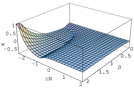
where ${\cal W}=\frac{\zeta}{2}\kappa^{2}{\phi^{\prime}}^{\,2}$. This class of solution is available only if $\phi\neq$ const, more precisely, if ${\cal W}^{\prime}+4{\cal W}\neq 0$. A solution satisfying ${\cal W}^{\prime}+4{\cal W}<2(y_{0}-2\sigma_{0})$, or with $\beta>4$, is inflating for all times (cf figure 1). Let us also restrict the solution by making the ansätz $\kappa\phi^{\prime}\equiv\sqrt{2/\zeta}\,\rm e^{-\beta\Delta N/2}$, where $\beta$ is arbitrary. In this case, the EoS parameter $w$ is less than $-1$ when

$$0<\kappa^{2}{\phi^{\prime}}^{\,2}<\frac{2}{\zeta}\,\frac{y_{0}-5\sigma_{0}-3}{5-\beta}.$$ (31)

If $\phi$ is rolling with a constant velocity, namely $\kappa\phi^{\prime}\equiv\sqrt{2\phi_{0}/\zeta}$, then $a\propto\rm e^{\sqrt{\zeta/2\phi_{0}}\,(\phi/m_{\rm Pl})}$; the scale factor grows exponentially with $\phi$. For the power-law expansion, $a(t)\propto t^{p}$, we get $\kappa\phi=\sqrt{\frac{2\phi_{0}}{\zeta}}\,p\ln t$ and $\kappa\sigma=\sqrt{\frac{2\sigma_{0}}{\gamma}}\,p\ln t$.

4.4 Absence of potential, $V(\sigma)=0$

In this subsection, we study the case where there is no potential for the field $\sigma$, and thus ${\cal Y}=0$. This corresponds to the case examined previously by Antoniadis, Rizos and Tamvakis [20] (see also  [28, 29]), who studied the system (7)-(10) numerically.

First, as a special case, we shall consider the solution $\varepsilon=\varepsilon_{0}$, or equivalently $a(t)\propto(c_{0}t+t_{1})^{p}$. The set of three independent equations of motion may be given by

$$\frac{\gamma}{2}\,\kappa^{2}{\sigma^{\prime}}^{\,2}=\rm e^{-(5+\varepsilon_{0})N}\left[c_{1}-\int\rm e^{(5+\varepsilon_{0})N}\left({\cal W}^{\prime}+(5+\varepsilon_{0}){\cal W}+3(1+\varepsilon_{0})\right){\rm d}N\right],$$

$$\kappa^{2}\sigma^{\prime}\xi_{,\,\sigma}H^{2}+\frac{\gamma\kappa^{2}}{6}\,{\sigma^{\prime}}^{\,2}=1+\frac{{\cal W}^{\prime}+(5+\varepsilon_{0}){\cal W}}{3(1+\varepsilon_{0})},$$ (32)

$$\kappa^{2}\phi^{\prime}\lambda_{,\,\phi}H^{2}=\frac{{\cal W}^{\prime}+2(3+\varepsilon_{0}){\cal W}}{3(1+\varepsilon_{0})},$$

where ${\cal W}\equiv\frac{\zeta}{2}\kappa^{2}{\phi^{\prime}}^{\,2}$, $\varepsilon_{0}\equiv-1/p$ and $c_{1}$ is an integration constant. In particular, for a logarithmic dilaton, $\phi(t)\propto\ln(c_{0}t+t_{1})$, and thus $\dot{\phi}/H=$ const $\equiv Q$, we get

$$\frac{\gamma}{2}\,\kappa^{2}{\sigma^{\prime}}^{\,2}=c_{1}\,\rm e^{(1/p-5)N}-\frac{\zeta}{2}\kappa^{2}Q^{2}-\frac{3(p-1)}{5p-1}.$$ (33)

Let us assume that $c_{1}$ is positive. There can exist some real differences between the cases $p>1$ and $p<1$, and also between $p>0$ and $p<0$. For $1/5<p<1$, the modulus field $\sigma$ normally behaves as a canonical scalar, even if $\zeta>0$, since $\kappa Q<1$. While, for $p>1$, and also for $p<0$, since the last term in (33) is negative, $\sigma$ may behave as a phantom field, especially for $N\gtrsim 0$.

In the following discussion, we analyze a simple and physically motivated case where the number of e-folds is proportional to a shift in field $\sigma$, namely $\kappa\sigma\equiv\sqrt{2\sigma_{0}/\gamma}\,N+$ const . In this case, the set of three independent equations of motion reads as

$$(1+\varepsilon)(2\sigma_{0}+{\cal U})+4\sigma_{0}=0,$$

$${\cal W}^{\prime}+4{\cal W}-\frac{4\sigma_{0}(2{\cal W}-3{\cal V})}{2\sigma_{0}+3{\cal U}}=0,$$ (34)

$$3({\cal V}-{\cal U})-{\cal W}-\sigma_{0}+3=0,$$

where ${\cal U}\equiv\kappa^{2}\sigma^{\prime}H^{2}\xi_{,\,\sigma}$ and ${\cal V}\equiv\kappa^{2}\phi^{\prime}\lambda_{,\,\phi}H^{2}$. It is not difficult to see that ${\cal U}=0$ implies only a decelerating universe; the combined effect of the (scalar) fields is such that the EoS parameter $w\equiv-1-2\varepsilon/3=1$, that is, the EoS for a stiff matter. However, with ${\cal U}\neq 0$, there exist other possibilities; for example, for $|{\cal U}|>2\sigma_{0}$, the universe is accelerating if ${\cal U}<0$. This acceleration can be super-luminal ($w<-1$), for $0>{\cal U}>-4\sigma_{0}$; this is consistent with the numerical results discussed in [20]. Below we shall study two more special cases.

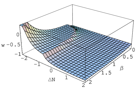
(i) Let us make the ansätz $\kappa(\dot{\phi}/H)\propto a^{\beta/2}$, more specifically, $\kappa\phi^{\prime}\equiv\sqrt{2/\zeta}\,\rm e^{-\beta(N-N_{0})/2}$, where $\beta$ is an arbitrary constant. A solution of this type, with $\beta\geq 5$, may be used for explaining a late-time acceleration of the universe. More specifically, for $\beta=5$, we find $w\sim-1$ when $N\lesssim N_{0}$ but $w>-1/3$ when $N>N_{0}$. For $\beta>5$, there exists a narrow range of $N$ where the EoS parameter $w$ falls between $-1$ and $-1/3$ (cf figure 2).

Figure 2: A non-constant dilaton case (cf equation (4.4)) with $\kappa\phi^{\prime}\propto\rm e^{-\beta(N-N_{0})/2}$. For $\beta>5$, there exists a crossing between the $w<-1$ and $w>-1$ phases, when $N\sim N_{0}$. The universe is not accelerating for any value of $\beta$ when $N\gtrsim N_{0}$. Here we have chosen $\sigma_{0}=1$, but the behaviour of the solution is not changed much in a wide range of $\sigma_{0}$ ($>0$).

(ii) Next, let us consider the asymptotic solution $\kappa\phi(t)\equiv\sqrt{\frac{2\phi_{0}}{\zeta}}\,\ln(a(t))+$ const. Then we find

$$\varepsilon=-1-\frac{4(\sigma_{0}+\phi_{0})}{3+\sigma_{0}+\phi_{0}},\qquad\kappa H^{2}\xi_{,\,\sigma}=\sqrt{\frac{\gamma\sigma_{0}}{2}}\,\left(1-\frac{\sigma_{0}}{3}-\frac{\phi_{0}}{\sigma_{0}+\phi_{0}}\right),$$

(35)

$$\kappa H^{2}\lambda_{,\,\phi}=\sqrt{\frac{\zeta\phi_{0}}{2}}\,\frac{\phi_{0}+\sigma_{0}-3}{3(\phi_{0}+\sigma_{0})}.$$

Acceleration is possible only if $-3<\sigma_{0}+\phi_{0}<0$, which requires that either $\phi_{0}<0$ or $\sigma_{0}<0$ (or both). This is essentially an example of phantom cosmology.

4.5 Small kinetic terms

Consider the case where the kinetic term for $\sigma$ is absent or it is negligibly small, $\dot{\sigma}/H\simeq 0$ . Then there exist two classes of solutions: the first one is given by

$$\phi^{\prime}\lambda_{,\,\phi}-\sigma^{\prime}\xi_{,\,\sigma}=\frac{1}{\kappa^{2}H_{0}^{2}}\left[\frac{c_{1}}{3}\,\rm e^{-4N}+\frac{c_{2}}{3}\,\rm e^{-2N}-\rm e^{2N}\right],$$

$$V(\sigma)=c_{1}\,\frac{H^{2}}{\kappa^{2}}\,\rm e^{2N},\qquad\kappa\phi^{\prime}=\sqrt{\frac{2c_{2}}{\zeta}}\,\rm e^{-2N}.$$ (36)

This is the critical solution with zero acceleration, $a\propto t$, or $H=H_{0}\,\rm e^{-N}$, implying that $V(\sigma)=$ const. The second solution may be obtained by solving the equations:

$${\cal W}=\rm e^{-\int(\varepsilon+5){{\rm d}N}}\left[c_{3}-\int\rm e^{(\varepsilon+5){\rm d}N}\left({\cal Y}^{\prime}+(\varepsilon-1){\cal Y}+3(1+\varepsilon)\right){{\rm d}N}\right],$$

(37)

$${\cal V}=-1+\frac{{\cal W}}{3}-\frac{{\cal Y}^{\prime}+(\varepsilon-1){\cal Y}}{3(1+\varepsilon)},\qquad{\cal U}=-\frac{{\cal Y}^{\prime}+2{\cal Y}\varepsilon}{3(1+\varepsilon)}.$$

In the case the kinetic term $\phi$ is also vanishingly small, $\phi^{\prime}\simeq 0$, so that ${\cal W}\simeq 0$, (4.5) yields

$$V(\sigma)=m_{Pl}^{2}H^{2}\exp\left[{\int(1-\varepsilon){\rm d}N}\right]\left(c_{3}-3\int(1+\varepsilon)\exp\left[-\int(1-\varepsilon){\rm d}N\right]{\rm d}N\right),$$

(38)

$$\sigma^{\prime}\xi_{,\,\sigma}=\frac{m_{Pl}^{2}}{H^{2}}-\frac{V(\sigma)}{3H^{4}},\qquad\phi^{\prime}\lambda_{,\,\phi}=0.$$

A prior knowledge about the time-dependence of the scale factor helps for retrieving the functional form of the potential $V(\sigma)$ (or vice versa). For the power-law expansion $H\propto\rm e^{\varepsilon_{0}N}$, we find

$$V(\sigma)\equiv V_{0}\,\rm e^{2\varepsilon_{0}N}+V_{1}\,e^{(1+\varepsilon_{0})N},\quad\xi(\sigma)\equiv\xi_{0}\,\rm e^{-\,2\varepsilon_{0}N}+\xi_{1}\,\rm e^{(1-3\varepsilon_{0})N},$$ (39)

where $V_{0}$ and $\xi_{0}$ may be (uniquely) determined, but $V_{1}$ and $\xi_{1}$ are arbitrary. Alternatively,

$$V(\sigma)\equiv V_{0}\,{a^{-2/\alpha}}+V_{1}\,{a^{-(1/\alpha-1)/\alpha}},$$ (40)

where $\alpha\equiv-1/\varepsilon_{0}$. This reveals an interesting possibility that during the matter domination era, $a\propto t^{2/3}$, the scalar potential may decrease (slowly) as $V\propto a^{-1/2}$ rather than the usual result $V\propto a^{-3}$. Moreover, in the presence of matter fields, this behaviour can change; in particular, with $c_{1}=0$, one finds $V\propto a^{-3(1+\bar{w})}$, where $\bar{w}$ characterizes the EoS parameter of a barotropic fluid.

4.6 Absence of modulus-GB coupling

Let us consider that ${\cal U}=0$ (or $\xi(\sigma)=0$) and also assume that $\sigma$ is rolling negligibly slow, $\dot{\sigma}\simeq 0$. In the absence of scalar potential, $V(\sigma)=0$, we find

$$\zeta{\phi^{\prime}}^{\,2}=\frac{2}{\kappa^{2}}\exp\left[-\int(5+\varepsilon){\rm d}N\right]\left(c_{1}-3\int(1+\varepsilon)\exp\left[\int(5+\varepsilon){\rm d}N\right]\,{\rm d}N\right),$$

(41)

$$\zeta{\phi^{\prime}}^{\,2}-6\phi^{\prime}H^{2}\lambda_{,\,\phi}=\frac{6}{\kappa^{2}},$$

where $c_{1}$ is an integration constant. These are the same set of equations as in (18), so we would not repeat our analysis for this case. With a non-trivial potential, $V(\sigma)\neq 0$, the system of equations reduces to

$$\zeta{\phi^{\prime}}^{\,2}=\frac{2}{\kappa^{2}}\,\sqrt{{\cal Y}}\,\rm e^{-5N}\left[c_{1}+\int\frac{({\cal Y}-3)(2{\cal Y}-{\cal Y}^{\prime})}{2{\cal Y}^{3/2}}\,\rm e^{5N}\,{\rm d}N\right],$$

(42)

$$\zeta{\phi^{\prime}}^{\,2}-6\phi^{\prime}H^{2}\lambda_{,\,\phi}=\frac{6}{\kappa^{2}}-2\Lambda_{0},$$

where ${\cal Y}=\Lambda_{0}\exp[-2\int\varepsilon dN]$. Typically, the rolling of $\sigma$ is proportional to the time variation of the scalar potential, but with $\dot{\sigma}=0$, $V(\sigma)=\Lambda_{0}/\kappa^{2}$. Especially, for the power-law expansion, $H\equiv H_{0}\,\rm e^{\varepsilon_{0}N}$ ($\varepsilon_{0}\neq-1$), we find

$$\frac{\zeta\kappa^{2}{\phi^{\prime}}^{\,2}}{2}=c_{1}\rm e^{-(5+\varepsilon_{0})N}-\frac{3(1+\varepsilon_{0})}{5+\varepsilon_{0}}+c_{2}\,\rm e^{-2\varepsilon_{0}N},$$ (43)

where $c_{2}$ is another integration constant. One may consider the possibility that $\varepsilon_{0}>0$, or $a(t)\propto(t_{\infty}-c_{1}t)^{\alpha}$ with $\alpha<0$, which implies a phantom like “equation of state”, $w<-1$. In the case the numerical coefficients $c_{1}$ and $c_{2}$ are positive, it is possible to attain $w<-1$ even with a canonical dilaton ($\zeta>0$).

4.7 Absence of GB terms

By ignoring the GB couplings, so that ${\cal U}=0$ and ${\cal V}=0$, one obtains perhaps the most canonical cosmological model with two scalars. If only $\sigma$ is evolving and $\phi$ is constant, then of course we find the standard result: ${\cal Y}=3+\varepsilon$, ${\cal X}=-\varepsilon$. However, if $\phi$ is also evolving, then these relations are modified as

$${\cal Y}=3+\varepsilon,\quad{\cal X}=-\varepsilon-{\cal W},\quad\varepsilon=-3-\frac{1}{2}\frac{{\cal W}^{\prime}}{{\cal W}}=-3-\frac{\phi^{\prime\prime}}{\phi^{\prime}}.$$ (44)

The implication of the additional field $\phi$ is clear: while the (functional) form of the potential is not changed, the kinetic term is modified. Let us discuss the result (44), in some detail. At the onset of inflation, $\varepsilon=-1$, one has $\phi\propto{1}/{a^{2}}$. During inflation, in at least some region of field space, $\varepsilon\to 0$ and hence $\phi\propto{1}/{a^{3}}$. Clearly, a linear dilaton background, $\phi(t)=\alpha+\beta\,t$, which implies $\phi^{\prime}=\beta/H$ and $\phi^{\prime\prime}=-\beta H^{\prime}/H^{2}$, is not a solution to the system of equations (44), while, a logarithmic dilaton background, $\phi\propto\ln t$, is clearly a solution. But this last ansätz implies, in conjunction with (44), that $a(t)\propto t^{1/3}$, which is clearly a non-accelerating solution.

If the system of equations (44) is to support a transition between $w<-1$ and $w>-1$ phases, then one needs to find a solution for $\phi$ such that its evolution takes the ratio $\phi^{\prime\prime}/\phi^{\prime}$ from $<-3$ to $>-3$ . The solution $\phi\propto 1/a^{\lambda}$ with $\lambda>2$ inflates forever. In particular, for the power-law expansion, $a\propto(c_{0}t+t_{1})^{\alpha}$ or $H\propto\rm e^{-N/\alpha}$, we get

$$\phi=\phi_{0}+\phi_{1}\,\rm e^{(-3+1/\alpha)N},\qquad{\sigma^{\prime}}^{\,2}=\frac{2}{\alpha\gamma\kappa^{2}}-\frac{\zeta}{\gamma}\,{\phi^{\prime}}^{\,2}.$$ (45)

It is possible (but not restricted) that $\phi$ and $\sigma$ both vary as $\kappa\phi\propto\sqrt{\frac{\alpha}{\zeta}}\,\ln t$, $\kappa\sigma\propto\sqrt{\frac{\alpha}{\gamma}}\,\ln t$; their combined effect may simply be that $V(\sigma)\propto 1/t^{2}\propto a^{-2/\alpha}$. In a matter dominated universe, this yields $V\propto 1/a^{3}$  [35, 12]. Of course, in the absence of GB couplings, there is no effect like $V(\sigma)\propto 1/\sqrt{a}$ coming from the second term in (40).

To summarize, we have seen that, with the standard approximation: $H(\sigma)\propto V^{1/2}(\sigma)$, $K(\sigma)\propto H^{2}(\sigma)$ and $\phi=$ const, the universe accelerates for $V>2K$ with the equation of state parameter $w>-1$. This result is independent of the strength of the modulus-GB coupling. If $\phi$ is non-constant, such as $\phi^{\prime}\propto\rm e^{-\beta\Delta N/2}$, a smooth crossing between $w<-1$ and $w>-1$ phases is possible for $\beta>4$. If the scalar potential, $V(\sigma)$, is vanishing, then such a crossing is possible only if $\phi$ is behaving as a phantom field and/or the quantity ${\cal U}$ ($\equiv\kappa^{2}\sigma^{\prime}H^{2}\xi_{,\sigma}$) changes its sign. Another interesting, as well as phenomenologically safe, example is $\dot{\sigma}\simeq 0$, that is the case with an almost constant modulus field. It is possible to attain $w<-1$ in this case by suitably choosing the integration constants (cf (43)), even if $\phi$ is canonical ($\zeta>0$). In the case when there are no GB-type corrections, the solutions with a non-constant dilaton are particularly interesting. The solution $\phi=\phi_{\infty}+\phi_{1}\,a^{-\lambda}$, with $\lambda>2$, inflates forever; since $w=1+\frac{2}{3}\frac{\phi^{\prime\prime}}{\phi^{\prime}}$, $\lambda=3$ corresponds to the case of a pure cosmological constant term, $w_{\Lambda}=-1$.

5 Second-order system

Let us introduce the following set of variables:

$${\cal X}=\frac{\gamma\kappa^{2}}{2}\left(\frac{\dot{\sigma}}{H}\right)^{2},\quad{\cal Y}=\kappa^{2}\frac{V(\sigma)}{H^{2}},\quad{\cal W}\equiv\frac{\zeta\kappa^{2}}{2}\left(\frac{\dot{\phi}}{H}\right)^{2},$$

(46)

$$\bar{\mathcal{U}}=\kappa^{2}\xi(\sigma)H^{2},\quad\bar{\mathcal{V}}=\kappa^{2}\lambda(\phi)H^{2},\quad\varepsilon=\frac{\dot{H}}{H^{2}}.$$

Note that $\bar{\mathcal{U}}$ and $\bar{\cal{V}}$ defined above are different from those in equation (4); here they do not involve derivatives in their definitions (see the appendix for additional details). These provide an alternative way to simplify the study of the model further. Equations (7)-(10) now form a different set of differential equations:

$$0=3(\bar{\mathcal{U}}^{\prime}-\bar{\mathcal{V}}^{\prime})-6\varepsilon(\bar{\mathcal{U}}-\bar{\mathcal{V}})+{\cal X}+{\cal W}+{\cal Y}-3,$$ (47)

$$0=\bar{\mathcal{V}}^{\prime\prime}-\bar{\mathcal{U}}^{\prime\prime}+(2-\varepsilon)(\bar{\mathcal{V}}^{\prime}-\bar{\mathcal{U}}^{\prime})-2(\bar{\mathcal{V}}-\bar{\mathcal{U}})(\varepsilon^{\prime}+\varepsilon^{2}+2\varepsilon)+{\cal X}+{\cal W}-{\cal Y}+2\varepsilon+3,$$ (48)

$$0={\cal X}^{\prime}+{\cal Y}^{\prime}+6{\cal X}+2\varepsilon({\cal X}+{\cal Y})+3(1+\varepsilon)(\bar{\mathcal{U}}^{\prime}-2\varepsilon\bar{\mathcal{U}}),$$ (49)

$$0={\cal W}^{\prime}+2(\varepsilon+3){\cal W}-3(\varepsilon+1)(\bar{\mathcal{V}}^{\prime}-2\varepsilon\bar{\mathcal{V}}).$$ (50)

Only equation (48) is second order in derivative, which can however be discarded since any solution following from the other three equations will automatically be satisfied by this equation.

In a constant dilaton background, for which ${\cal W}=0$, the above system of equations simplify further. There are broadly three different classes of solutions:

$$(i) \quad\bar{\mathcal{V}}=0,\qquad\quad\varepsilon=\varepsilon(N),$$ (51)

$$(ii) \quad\bar{\mathcal{V}}=\bar{\mathcal{V}}(N),\qquad\varepsilon=\frac{\bar{\mathcal{V}}^{\prime}}{2\bar{\mathcal{V}}},$$ (52)

$$(iii) \quad\bar{\mathcal{V}}=\bar{\mathcal{V}}(N),\qquad\varepsilon=-1.$$ (53)

The first branch, (51), corresponding to the case with no dilaton-dependent terms was analyzed before in [23]. The second branch, (52), implies $\bar{\mathcal{V}}\propto H^{2}$ and thus $\lambda(\phi)=$ const. The first two branches satisfy

$$\frac{\bar{\mathcal{U}}^{\prime\prime}}{2}+\frac{5-\varepsilon}{2}\,\bar{\mathcal{U}}^{\prime}-(\varepsilon^{\prime}+\varepsilon^{2}+5\varepsilon)\bar{\mathcal{U}}=3+\varepsilon-{\cal Y},$$ (54)

$$\frac{\bar{\mathcal{U}}^{\prime\prime}}{2}-\frac{1+\varepsilon}{2}\,\bar{\mathcal{U}}^{\prime}-(\varepsilon^{\prime}+\varepsilon^{2}-\varepsilon)\bar{\mathcal{U}}=\varepsilon+{\cal X},$$ (55)

while, the third branch satisfies

$$\frac{1}{2}(\bar{\mathcal{V}}^{\prime\prime}-\bar{\mathcal{U}}^{\prime\prime})+3(\bar{\mathcal{V}}^{\prime}-\bar{\mathcal{U}}^{\prime})+4(\bar{\mathcal{V}}-\bar{\mathcal{U}})={\cal Y}-2,$$

$$\frac{1}{2}(\bar{\mathcal{V}}^{\prime\prime}-\bar{\mathcal{U}}^{\prime\prime})+2(\bar{\mathcal{V}}-\bar{\mathcal{U}})=-{\cal X}+1.$$ (56)

This is actually the critical case with zero acceleration.

5.1 Inflating without a scalar potential

In this subsection we show that in our model it is possible to achieve a cosmic inflation without a scalar potential. For simplicity, let us also drop all $\phi$-dependent terms and work momentarily in terms of the original variables ($x$, $\bar{u}$ and $\varepsilon$) and in the units $\kappa=1$. Recall that

$$\bar{u}\equiv\xi(\sigma)H^{2}$$ (57)

This quantity should normally decrease with the expansion of the universe, so that all higher order corrections to Einstein’s theory are only sub-leading . With $V(\sigma)=0$, the equations of motion reduce to the form

$$\gamma x^{2}=6-6\bar{u}^{\prime}+12\varepsilon\bar{u},\quad\varepsilon^{\prime}+\varepsilon(\varepsilon+5)=\frac{\bar{u}^{\prime\prime}+(5-\varepsilon)\bar{u}^{\prime}}{2\bar{u}}-\frac{\bar{u}}{\varepsilon}.$$ (58)

Fixing the (functional) form of $\bar{u}$ would alone give a desired evolution for $\varepsilon$. In particular, for $\bar{u}\simeq$ const $=\bar{u}_{0}\neq 0$, the explicit solution for $\varepsilon$ is given by

$$\varepsilon=-\beta_{0}+\beta\tanh\left(\beta\Delta N\right),$$ (59)

where $\Delta N=N+C$, with $C$ being an integration constant, and

$$\beta_{0}\equiv\frac{5\bar{u}_{\lower 2.0pt\hbox{$\scriptstyle 0$}}+1}{2\bar{u}_{\lower 2.0pt\hbox{$\scriptstyle 0$}}},\quad\beta\equiv\frac{1}{2\bar{u}_{\lower 2.0pt\hbox{$\scriptstyle 0$}}}\sqrt{25\bar{u}_{\lower 2.0pt\hbox{$\scriptstyle 0$}}^{2}-2\bar{u}_{\lower 2.0pt\hbox{$\scriptstyle 0$}}+1}.$$ (60)

The evolution of $\sigma$ is given by $\sigma^{\prime}=\pm\sqrt{(6+12\varepsilon\bar{u}_{\lower 2.0pt\hbox{$\scriptstyle 0$}})/\gamma}$. The Hubble parameter is given by

$$H=H_{0}\,\rm e^{-\beta_{0}N}\cosh(\beta\Delta N).$$ (61)

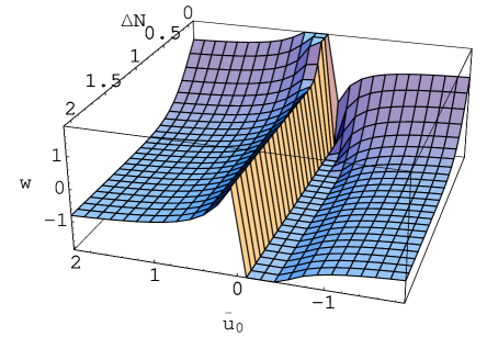
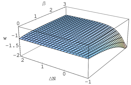
For $\bar{u}_{\lower 2.0pt\hbox{$\scriptstyle 0$}}>0$, both $\beta_{\lower 2.0pt\hbox{$\scriptstyle 0$}}$ and $\beta$ are positive and $\beta_{\lower 2.0pt\hbox{$\scriptstyle 0$}}>\beta$, implying that $H$ decreases with the number of e-folds, and, in turn $w>-1$. However, for $\bar{u}_{\lower 2.0pt\hbox{$\scriptstyle 0$}}<0$, we get $\beta<0$, whereas $\beta_{\lower 2.0pt\hbox{$\scriptstyle 0$}}<0$ for $-0.2<\bar{u}_{\lower 2.0pt\hbox{$\scriptstyle 0$}}<0$ and $\beta_{\lower 2.0pt\hbox{$\scriptstyle 0$}}>0$ for $\bar{u}_{\lower 2.0pt\hbox{$\scriptstyle 0$}}<-0.2$. Clearly, with $\bar{u}_{\lower 2.0pt\hbox{$\scriptstyle 0$}}<0$, a solution of type (59) allows the value $\varepsilon>0$ or $w<-1$ (cf figure 3).

Figure 3: The EoS parameter $w$ ($\equiv-1-2\varepsilon/3$) as a function of $\bar{u}_{\lower 2.0pt\hbox{$\scriptstyle 0$}}$ and $N$. For $\bar{u}_{\lower 2.0pt\hbox{$\scriptstyle 0$}}<0$, we get a super-inflationary solution, $\dot{H}/H^{2}>0$, which corresponds to the $\delta<0$ case first studied in [20]. Interestingly, for $\bar{u}\simeq$ const, it is possible to get a cosmic inflation of an arbitrary magnitude even for $\delta>0$ (or $\bar{u}>0$) without violating the null energy condition. Of course, $w>-1$ in this case.

5.2 Quintessence/phantom crossing

Within the best-fit concordance cosmology the present observational data seem to slightly favour a dynamical dark energy with $w_{de}$ crossing $-1$ from above to below, when the red-shift factor $z\lesssim 0.6$ [36]. Could it be that our universe crosses the phantom divide , $w=-1$, only recently? And could it be due to a GB-type modification of general relativity? This is indeed an interesting subject of recent discussion on both fronts: observational [36] and theoretical  [37] cosmology. Though a more detailed analysis of the model, accommodating the effects due to matter fields, is needed yet, first indications are that such a possibility cannot be denied.

First we consider the case where the modulus field $\sigma$ is behaving similarly to the dilaton $\phi$, so $\bar{\mathcal{V}}=\bar{\mathcal{U}}$. Then there are again three different classes of solutions:

$$(i)\quad {\cal X}=-\varepsilon,~{}~{}\qquad{\cal Y}=3+\varepsilon,~{}~{}\qquad\bar{\mathcal{U}}=0,$$ (62)

$$(ii)\quad {\cal X}=-\frac{\bar{\mathcal{U}}^{\prime}}{\bar{\mathcal{U}}},\qquad{\cal Y}=3+\frac{\bar{\mathcal{U}}^{\prime}}{2\bar{\mathcal{U}}},\qquad\varepsilon=\frac{\bar{\mathcal{U}}^{\prime}}{2\bar{\mathcal{U}}},$$ (63)

$$(iii)\quad {\cal X}=1,\qquad{\cal Y}=2,\qquad\varepsilon=-1.$$ (64)

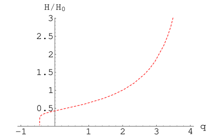
The first branch is the standard one, implying that $\lambda(\phi)=0=\xi(\sigma)$, while the third branch gives zero acceleration, so it is the second branch which is most interesting. For $H\propto\left(\xi(\sigma)\right)^{-1/2}$, so that $\bar{\mathcal{U}}=$ const, the effect is similar to that of a pure cosmological constant term, $\varepsilon=0$. Instead, if $H\propto\left(\xi(\sigma)\right)^{-1/2}a^{-\,\alpha/2}$, then the universe is accelerating for $\alpha<2$, whereas $\alpha=2$ marks the boarder between acceleration and deceleration. Typically, for the solution $\bar{\mathcal{U}}=c_{1}N+c_{2}$ (with $c_{i}>0$) we find $\varepsilon<0$ for $N<-c_{2}/c_{1}$ and $\varepsilon>0$ for $N>-c_{2}/c_{1}$, where $N\equiv\ln(a(t)/a_{0})$, with $a_{0}$ being the present value of $a(t)$, and $1+z\equiv\rm e^{\Delta N}$. For instance, if $c_{2}/c_{1}=0.47$, then the EoS parameter $w$ is less than $-1$ for $z<0.6$.

5.3 Deceleration/acceleration phase and crossing of phantom divide

Consider the possibility that the coupling functions $\xi(\sigma)$ and $\lambda(\phi)$ both vary inversely with $H^{2}$, so that $\bar{\mathcal{U}}\equiv u_{0}$ and $\bar{\mathcal{V}}\equiv v_{0}$. For $u_{0}=v_{0}$ (which again implies a trivial GB coupling), there are three different classes of solutions. The first class of solution is given by

$$\varepsilon=-3+\sqrt{6}\tanh\sqrt{6}\,\Delta N,\quad V\propto\rm e^{-\,6N}\,\sinh 2\sqrt{6}\,\Delta N,$$

$$\gamma{\sigma^{\prime}}^{\,2}=\frac{2}{\kappa^{2}}\,\left[(6v_{0}-1)\tanh\sqrt{6}\,\Delta N-3(5v_{0}-1)\right],$$ (65)

$$\zeta{\phi^{\prime}}^{\,2}=-\frac{6}{\kappa^{2}}\,v_{0}\left(2\sqrt{6}\tanh\sqrt{6}\,\Delta N-5\right),$$

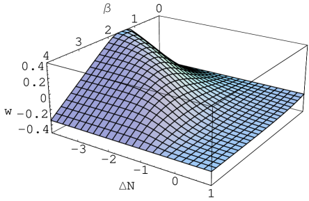
where $\Delta N\equiv N+N_{1}$. This solution yields only a standard inflation for which $\varepsilon<0$ (cf figure 4). The transition from the deceleration phase to the acceleration phase (or vice verse) is a natural ingredient of the above solution. In fact, we would not have gained such an insight into a functional from of $\varepsilon$ (and the EoS parameter $w$), have we had dropped the GB couplings from the action, which corresponds to the case $v_{0}=0$.

For $|\Delta N|\gtrsim 1$, since $|\tanh\sqrt{6}\Delta N|\simeq 1$, both the fields $\sigma$ and $\phi$ are rolling with almost constant velocities, viz, $\sigma\equiv\sigma_{0}\sqrt{6}\,N$, where $\sigma_{0}\equiv m_{Pl}\sqrt{(2-9v_{0})/3\gamma}$. The scalar potential and the modulus GB coupling take the following form

$$V(\sigma) = V_{0}\,\rm e^{-\,\sqrt{6}(\sigma/\sigma_{0})}\,\sinh 2\left(c+\sigma/\sigma_{0}\right),$$

$$\xi(\sigma) = \xi_{0}\,\rm e^{\sqrt{6}(\sigma/\sigma_{0})}\,\left[\cosh\left(c+\sigma/\sigma_{0}\right)\right]^{-\,2},$$ (66)

where $c$ is an arbitrary constant. A similar expression may be given for $\lambda(\phi)$, in terms of $\phi$.

Figure 4: The universe enters into an accelerating phase ($\varepsilon>-1$) when $\Delta N\simeq 0.22$, or $H/H_{0}\simeq 0.42$ (cf equation (5.3)). For $\Delta N\gtrsim 1$, the field $\phi$ is almost constant, with the deceleration parameter $q\equiv-1-\varepsilon\simeq-0.45$ and $w\simeq-0.63$.

Figure 5: The equation of state parameter $w~{}(\equiv-1-2\varepsilon/3)$ with $\kappa\phi^{\prime}\equiv\sqrt{\frac{2\phi_{0}}{\gamma}}\,\rm e^{-\beta(N-N_{0})/2}$ and $\phi_{0}/v_{0}=0.2$ (cf the negative root in equation (68)). Only a small value of $\beta$ seems to be reasonable, otherwise $w$ can be imaginary for $\Delta N\ll 0$.

Figure 6: The equation of state parameter $w$ as in figure 6, but for the positive root in equation (68). For $\beta>0$, the universe passes from a decelerating phase to an accelerating phase, but does not cross the phantom divide, $w=-1$.

Figure 7: The equation of state parameter $w$ with $\kappa\phi^{\prime}\equiv\sqrt{\frac{2\phi_{0}}{\gamma}}\,\rm e^{-\beta(N-N_{0})/2}$ and $\phi_{0}/v_{0}=-0.2<0$ (cf the negative root in equation (68)). Here $w$ may start from a value (well) below $-1$ but it never crosses it, leading always to a phantom phase.

Figure 8: The equation of state parameter $w$ as in figure 7, but for the positive root in equation (68). For any value of $\beta$, the universe is not accelerating, since in this case $w$ always takes a value larger than $-1/3$.

The other two classes of solutions may be described by the following system of equations:

$${\cal X}=-\varepsilon-{\cal W},\quad{\cal Y}=3+\varepsilon,$$ (67)

where, as above, ${\cal W}\equiv\frac{\zeta}{2}\kappa^{2}{\phi^{\prime}}^{\,2}$, and

$$\varepsilon=-\frac{1}{2}-\frac{{\cal W}}{6v_{0}}\pm\frac{1}{6}\sqrt{9+\left(\frac{{\cal W}}{v_{0}}\right)^{2}-\frac{6{\cal W}^{\prime}}{v_{0}}-\frac{30{\cal W}}{v_{0}}}.$$ (68)

In the constant dilaton case, $\phi^{\prime}=0$, we find $w=-1$ or $0$. We assume that we are dealing with a canonical dilaton, so ${\cal W}>0$. For ${\cal W}/\bar{\mathcal{V}}_{0}>0$, the both roots in (68) give the EoS parameter $w>-1$. However, for ${\cal W}/\bar{\mathcal{V}}_{0}<0$, the positive root can give $w<-1$.

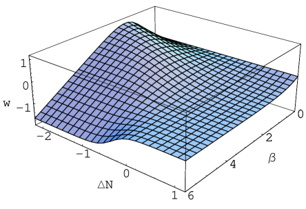
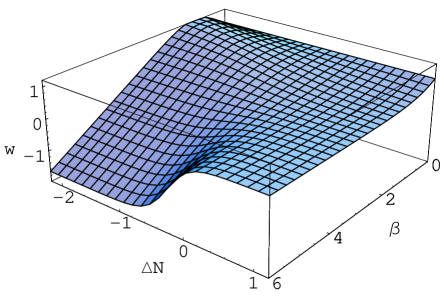
To simplify the analysis further, let us make the ansätz $\kappa\phi^{\prime}\equiv\sqrt{\frac{2\phi_{0}}{\gamma}}\,\rm e^{-\beta\Delta N/2}$, where $\beta$ is arbitrary. Then, for $\phi_{0}/v_{0}>0$, in the regime $\Delta N\gg 0$, such that $\phi^{\prime}/\phi_{0}\to 0$, the positive root in (68) yields $w\sim-1$ (except for $\beta\simeq 0$), while the negative root yields $w\sim-1/3$ (see figures 5 and 6). On the other hand, for ${\cal W}/v_{0}<0$, the positive root supports a phantom phase ($w<-1$), while the negative root solution is not accelerating, as it approaches $w=-1/3$ from above (see figures 7 and 8). It is generally for $u_{0}<0$ (or equivalently $v_{0}<0$ or $\delta<0$) that one of the branches can give a non-standard ($w<-1$) or super-inflationary phase satisfying $p+\rho<0$, in consistent with the numerical results in  [20, 28].

For the power-law expansion, $a(t)\propto t^{\alpha}$, so that $H=\alpha/t$, and $\phi^{\prime}=$ const (or $\phi\propto\ln t+$ const), we require $\phi_{0}/v_{0}<0.30$ or $>29.69$ so as to keep $\varepsilon$ real. We shall be interested in the case where $v_{0}$ is small, so that the GB contribution is only sub-leading. For instance, if ${\cal W}\simeq-0.1v_{0}>0$, then $\varepsilon\simeq-1.06$ or $0.09$; only the second branch is accelerating which gives $w\simeq-1.06$.

In the $u_{0}\neq v_{0}$ case, so that the GB coupling is non-vanishing, the first branch, (5.3), is modified as

$$\gamma{\sigma^{\prime}}^{\,2}=\frac{2}{\kappa^{2}}\left[(7u_{0}-v_{0}+1)(3+\varepsilon)-3(6u_{0}-v_{0}-1)\right],$$

$$V=m_{Pl}^{2}(v_{0}-u_{0}+1)(3+\varepsilon)\,H^{2}$$ (69)

without changing the forms of ${\cal W}$ and $\varepsilon$. As for the second branch, (68), the expressions of $\gamma{\sigma^{\prime}}^{\,2}$ and $V(\sigma)$ are now more complicated and not illuminating at least to write down here. However, a simplification occurs in the case that $H\equiv H_{0}\,\rm e^{\varepsilon_{0}N}$ or equivalently, $a\propto(c_{0}t+t_{1})^{\alpha}$ ($\alpha>0$) or $a\propto(t_{\infty}-t)^{-\alpha}$ ($\alpha<0$). Especially, the time variations of the scalar fields are given by

$$\gamma{\sigma^{\prime}}^{\,2}=\frac{2}{\kappa^{2}}\bigg{[}-c_{1}\rm e^{-2(3+\varepsilon_{0})N}+\frac{3(1+\varepsilon_{0})\varepsilon_{0}u_{0}}{3+\varepsilon_{0}}+\varepsilon_{0}(1-\varepsilon_{0})(u_{0}-v_{0})-\varepsilon_{0}\bigg{]},$$

$$\zeta{\phi^{\prime}}^{\,2}=\frac{2}{\kappa^{2}}\left[c_{1}\rm e^{-2(3+\varepsilon_{0})N}-\frac{3(1+\varepsilon_{0})\varepsilon_{0}u_{0}}{3+\varepsilon_{0}}\right].$$ (70)

Here either value of $\varepsilon_{0}$ is possible; for $\varepsilon_{0}>0$, $\phi$ may behave as a phantom field, especially, if $N>0$ and/or $c_{1}<0$, unless that $u_{0}$ (or $\xi(\sigma))$ is negative.

5.4 Late-time approximation: two scalar case

Finally, as a good approximation at late times, consider that one of the fields, mainly $\sigma$, is rolling very slow such that $\kappa|\sigma^{\prime}|\equiv\sqrt{2x_{0}/\gamma}$ and $\kappa H^{-1}(\sigma)\equiv\sqrt{y_{0}}\,V^{-1/2}(\sigma)$, where $x_{0}$ is a small constant, while $y_{0}>0$. In the case of a vanishing effective GB coupling, $\bar{\mathcal{U}}=\bar{\mathcal{V}}$, the system of equations reduce to

$$H^{2}=\frac{1}{\kappa^{2}\xi(\sigma)}\left[c_{1}\,\rm e^{-2(3-y_{0})N}-\frac{y_{0}(x_{0}+y_{0}-3)}{3(y_{0}-2)(3-y_{0})}\right],$$

$$\zeta{\phi^{\prime}}^{\,2}=\frac{2}{\kappa^{2}}\left(3-x_{0}-y_{0}\right),\quad\varepsilon=y_{0}-3.$$ (71)

The universe accelerates for $y_{0}>2$. An especially interesting range for $y_{0}$ is $2<y_{0}<3$, for which the universe naturally undergoes a cosmic acceleration and the couplings $\xi(\sigma)$ and $\lambda(\phi)$ both decrease exponentially with the number of e-folds, $N$.

In the general case, there are five different branches of solutions: except the first branch, which is giving by

$$\xi(\sigma)=0,\quad\varepsilon=-\frac{3x_{0}}{x_{0}+y_{0}},$$

$$\zeta{\phi^{\prime}}^{\,2}=\frac{2}{\kappa^{2}}\left[c_{1}\,\rm e^{-(2+\varepsilon)N}+\frac{(2x_{0}-y_{0})(3-x_{0}-y_{0})}{2x_{0}+5y_{0}}\right],$$ (72)

$$H^{2}=\frac{1}{\kappa^{2}\lambda(\phi)}\,\rm e^{-6x_{0}N/(x_{0}+y_{0})}\bigg{[}c_{2}-\int\rm e^{6x_{0}N/(x_{0}+y_{0})}\left(3-x_{0}-y_{0}-\frac{\zeta}{2}\,\kappa^{2}{\phi^{\prime}}^{\,2}\right){\rm d}N\bigg{]},$$

their expressions are lengthy and not illuminating at least to write down here. However, especially, for $\varepsilon\equiv\varepsilon_{0}$, they merge to give a single solution

$$\zeta{\phi^{\prime}}^{2} = \frac{2}{\kappa^{2}}\left[\frac{y_{0}(1-\varepsilon_{0})-3(1+\varepsilon_{0})}{5+\varepsilon_{0}}-x_{0}-3\lambda_{1}(5+3\varepsilon_{0})\right],$$

$$\xi(\sigma) = \frac{1}{\kappa^{2}H_{0}^{2}}\left(\,\xi_{0}+\xi_{1}\,\rm e^{-\,2\varepsilon_{0}N}\right),$$ (73)

$$\lambda(\phi) = \frac{1}{\kappa^{2}H_{0}^{2}}\left(\,\lambda_{0}+\lambda_{1}\,\rm e^{-(5+3\varepsilon_{0})N}+\lambda_{2}\,\rm e^{-\,2\varepsilon_{0}N}\right),$$

where $\xi_{0}$, $\lambda_{0}$ and $\lambda_{1}$ are integration constants, and

$$\xi_{1} \equiv \frac{3x_{0}+(x_{0}+y_{0})\varepsilon_{0}}{3\varepsilon_{0}(1+\varepsilon_{0})},$$

$$\lambda_{2} \equiv \frac{(3+\varepsilon_{0})[(3+x_{0}+y_{0})\varepsilon_{0}+3+5x_{0}-y_{0}]}{3\varepsilon_{0}(5+\varepsilon_{0})(1+\varepsilon_{0})}$$ (74)

with $\varepsilon_{0}\neq-1$. One may replace $N$ by $\sqrt{\frac{\gamma}{2x_{0}}}\,\kappa\sigma$ so as to retrieve a functional form for $\xi(\sigma)$. Especially, the cases $\varepsilon_{0}=0,-5$ (and also $\varepsilon_{0}=-5/3$) need to be treated separately, for which new terms appear with $N$-dependence. For instance, for $\varepsilon_{0}=0$ (i.e. $H\equiv H_{0}$), we find

$$\zeta{\phi^{\prime}}^{\,2}=\frac{2}{\kappa^{2}}\left[\frac{y_{0}-3}{5}-x_{0}+c_{1}\,\rm e^{-\,5N}\right],$$

$$\lambda(\phi)=\frac{1}{\kappa^{2}H_{0}^{2}}\left[\lambda_{0}-\frac{\lambda_{1}}{15}\,\rm e^{-\,5N}-\frac{2}{5}(5x_{0}+3-y_{0})N\right],$$ (75)

$$\xi(\sigma)=\frac{1}{\kappa^{2}H_{0}^{2}}\left[\xi_{0}-2x_{0}N\right]\equiv\frac{1}{\kappa^{2}H_{0}^{2}}\,\left[\xi_{1}-\sqrt{2\gamma x_{0}}\,\kappa\sigma\right].$$

With no surprise, this solution behaves all the times as a cosmological constant term, for which $w=-1$, since $H\equiv H_{0}$ and $V(\sigma)=m_{Pl}^{2}H_{0}^{2}y_{0}^{2}\equiv\Lambda$.

We conclude this section by providing an overview of the different solutions discussed above. In subsection 5.1 we showed the existence of an inflationary solution with a vanishing potential and for the modulus-GB coupling $\xi(\sigma)\propto H^{-2}$. This result is quite interesting. It is also obvious from the above analysis that solutions with trivial scalar-GB couplings ($\bar{\cal U}=0=\bar{\cal V}$) are not equivalent to solutions where these coupling are (negligibly) small, at late times. The simplest way to visualize this is to set only $\tilde{\cal U}=\tilde{\cal V}$, i.e., the dilaton $\phi$ is behaving as the modulus $\sigma$. Unlike in the $\bar{\cal U}=0=\bar{\cal V}$ case, we now find three different kinds of solutions, one of which, namely (63) can support a crossing between $w<-1$ and $w>-1$ cosmologies. When $\lambda(\phi)$ and $\xi(\sigma)$ both grow inversely with the squared of the Hubble parameter, $H^{2}$, then, for the first branch, the EoS parameter $w$ can take a value less than $-1/3$, namely $w\simeq-0.63$ at late times. Either both of the other two branches support an inflationary phase with $w>-1$, or only one of the branches supports an inflationary phase, but with $w<-1$. In the latter case, the second branch is not accelerating since $\varepsilon<-1$.

As in the standard picture, with $H\propto V^{1/2}$ and $\dot{\sigma}\propto H(\sigma)$, the universe accelerates for $y_{0}\equiv\kappa^{2}\frac{V(\sigma)}{H^{2}}>2$, even if $\bar{\cal U}=\bar{\cal V}\neq 0$. This result is independent of the ratio $\dot{\sigma}/H$. It is the case for $y_{0}<3$, the function $\bar{\cal U}$ decreases with the expansion of the universe. In the general case, for which $\bar{\cal U}\neq\bar{\cal V}\neq 0$, there are five branches of solutions, which simplify, for instance, if we take the limit where the slow-roll type variable $\varepsilon$ is constant.

6 Runway dilaton and matter coupling

In a more realistic scenario, $V(\sigma)$ in (6) may be replaced by a general form of the potential, namely

$$V(\sigma)\to V(\phi,\sigma)=\tilde{\lambda}(\phi)V(\sigma),$$

which is now a function of both the modulus $\sigma$ and the dilaton $\phi$. In our analysis we considered only the simplest case where $\phi$ was expected to evolve (relatively fast) towards its finite value $\phi_{m}$. In this limit, $\tilde{\lambda}(\phi)\simeq{\rm const}$.

Generally, $\phi$ (the spin-$0$ partner of spin-$2$ graviton) is coupled to Einstein term and thus, while going from string frame to Einstein frame, it may also couple to matter fields. In the heterotic string theory studied by Antoniadis, Gava and Narain [19], there is no coupling between the field $\sigma$ and the Ricci-scalar term, so $\sigma$ couples to gravity only via spacetime curvature tensors or Riemann curvature invariants. Thus a conformal transformation does not necessarily involve a $\sigma$-dependent term, but only a dilaton dependent term. In addition, $\sigma$ generally has a non-zero vacuum expectation value and hence a non-zero mass [20]; it is thus conceivable to expect only a minimal coupling between $\sigma$ and the matter. Furthermore, in a de Sitter (accelerating) universe, sypersymmetry has to be broken in general. If so, dilaton acquires a large enough mass ($m_{\phi}\gtrsim 10^{-3}{\rm eV}$) after supersymmetry breaking. Within this scenario, $\phi$ takes an almost constant value and hence it decouples from matter, so called least coupling principle [38, 39]. In any case, let us assume that $\phi$ is coupled to matter fields non-minimally:

$$S=\int d^{4}{x}\sqrt{-g}\bigg{[}\frac{1}{2\kappa^{2}}R-\frac{\gamma}{2}(\nabla\sigma)^{2}-V(\sigma)-\frac{\zeta}{2}(\nabla\phi)^{2}+\frac{f}{8}\,{\cal R}^{2}_{GB}+A^{4}(\phi)\left(\rho_{M}+\rho_{R}\right)\bigg{]},$$ (76)

where $f\equiv[\lambda(\phi)-\delta\xi(\sigma)]$. The equations of motion that describe gravity, the scalars, and the matter and radiation are given by (in units $\kappa=1$)

$$H^{2}=\frac{1}{3}\left(\frac{\gamma}{2}\dot{\sigma}^{2}+\frac{\zeta}{2}\dot{\phi}^{2}+V-3H^{3}\dot{f}+A^{4}(\rho_{M}+\rho_{R})\right),$$ (77)

$$\frac{\ddot{a}}{a}=-\frac{1}{3}\bigg{[}\gamma\dot{\sigma}^{2}+\zeta\dot{\phi}^{2}-V+A^{4}\rho_{R}+\frac{1}{2}A^{4}\rho_{M}+\frac{3}{2}\,H^{2}\left(H\dot{f}+\ddot{f}+2\dot{f}\dot{H}/H\right)\bigg{]},$$ (78)

$$\gamma(\ddot{\sigma}+3H\dot{\sigma})=-V_{,\,\sigma}-\frac{1}{8}\,\xi_{,\,\sigma}\,{\cal R}^{2}_{GB},$$ (79)

$$\zeta(\ddot{\phi}+3H\dot{\phi})=-A_{,\,\phi}A^{3}\,\rho_{M}+\frac{1}{8}\,\lambda_{,\,\phi}\,{\cal R}^{2}_{GB},$$ (80)

In the standard scenario of no matter-scalar coupling, e.g. the model of quintessence, $A(\phi)=1$. For $A(\phi)\neq 1$, the fluid equation of motion for matter (or radiation) is

$$a\frac{\partial\rho_{i}}{\partial a}+\frac{1}{\tilde{\alpha}}\,\frac{\partial\rho_{i}}{\partial\phi}=-3(\rho_{i}+p_{i}),$$ (81)

where $i=M({\rm matter})$ or $R({\rm radiation})$ and $\tilde{\alpha}\equiv\frac{d\ln A}{d\phi}$. The implicit assumption is that matter couples to $A^{2}(\phi)g_{\mu\nu}$ (with scale factor $\hat{a}$) rather than the Einstein metric $g_{\mu\nu}$ alone, and $\rho_{R}\propto 1/\hat{a}^{4}$, where $\hat{a}\equiv aA(\phi)$ so only $\rho_{M}$ enters the $\phi$ equation of motion. We can practically drop the $\rho_{R}$ term, at late times, since most of the radiation energy in the universe is in the cosmic microwave background, which makes up a fraction of roughly $5\times{10}^{-5}$ of the total density of the universe.

In the case $A(\phi)=1$, one can solve the system of equations (77)-(81), for example, by making an ansätz for the evolution of one of the scalars and/or the scale factor of the universe. Note that in this case the energy conservation equation (81) is easily expressed as a differential equation, namely $\Omega_{i}^{\prime}+2\varepsilon\Omega_{i}+3(1+w_{i})\Omega_{i}=0$, where $\Omega_{i}\equiv\rho_{i}/3H^{2}$, $w_{i}\equiv p_{i}/\rho_{i}$ and $\Omega^{\prime}={\rm d}\Omega/{\rm d}\ln[a(t)]$. In the case $A(\phi)\neq 1$, the extra (matter) degree of freedom added to the model complicates the problem, in which case the field equations may be solved numerically [40].

Especially in the case where $\phi$ evolves considerably slow with time, $A(\phi)$ is not essentially a constant, even at late times. In this case, a question may be raised as to whether the equivalence principle (universality of free fall in a given gravitational field) is violated due to a runway dilaton [38, 39], leading to time variations of some of the fundamental constants, like the fine structure constant $\alpha_{e}=e^{2}/\hbar c$. For metrically coupled matter theories, one may also raise a question regarding the time variation of Newton’s constants under post-Newtonian approximation [41]. But the constraints on gravitational actions of the type considered here, under (post-)Newtonian approximations, may be less stringent as they only require [42, 43] (in units $\kappa=1$)

$$\dot{\sigma}H^{2}\frac{d\xi(\sigma)}{{\rm d}\sigma}<{10}^{-2},\qquad\dot{\phi}H^{2}\frac{{\rm d}\lambda(\phi)}{{\rm d}\phi}<{10}^{-2}.$$ (82)

In our notations, introduced in equation (4), these read ${\cal U}H<{10}^{-2}$ and ${\cal V}H<{10}^{-2}$. This result does not rule out any scalar-GB couplings. Within our model, both ${\cal U}$ and ${\cal V}$ may be exponentially small (close to zero). In any case, if ${\cal U}\sim H^{2}\frac{d\xi(\sigma)}{{\rm d}\sigma}\sim{\cal O}(1)$ and ${\cal V}\sim H^{2}\frac{d\lambda(\phi)}{{\rm d}\phi}\sim{\cal O}(1)$, then we would require that $\dot{\sigma},\dot{\phi}<{10}^{-2}$ (in units $\kappa=1$).

If $\lambda(\phi)$ and $\xi(\sigma)$ are nearly constants, especially, after inflation, which we assume to be the case here, then action (76) may be compared to the gravitational action considered in [38] (cf equation (2.4)), under the replacement, $V(\sigma)\to V(\phi,\sigma)=\tilde{\lambda}(\phi)V(\sigma)$. For most of the solutions that we have presented in this paper, after a certain number of e-folds of expansion, the rolling of $\phi$ could be small as it is given by $\phi^{\prime}=\sqrt{\frac{2{\cal W}}{\zeta}}H\sim\rm e^{-\,\beta N}$ with $\beta N>0$. In a specific model considered in [38], $\tilde{\lambda}(\phi)\equiv\lambda_{\infty}(1+b_{\lambda}\rm e^{-\,c\phi})$, for $\frac{\dot{\phi}}{H}=\phi^{\prime}<0.7$, the level of variation of fine structure constant, $|d\ln e^{2}/dt|\lesssim 10^{-21}{\rm yr}^{-1}$ is much smaller than the current best limit on the time variation of $e^{2}$, namely $|d\ln e^{2}/dt|\lesssim 10^{-17}{\rm yr}^{-1}$; thus, a small rolling of $\phi$ is physically viable and phenomenologically acceptable.

One may be more concerned here with a time-variation of the (common) modulus $\sigma$. We take $\dot{\sigma}=0$ as a conservative case, for which $V(\sigma)$ is also constant (cf equation (4.6)). Because of phenomenological reasons it is desirable that the rolling of $\sigma$ is small, especially after inflation, which then allows only a slow rolling of the potential. Instead of the condition $\dot{\sigma}=0$, we expect $\kappa\dot{\sigma}<H$ to hold at all times, i.e. $\sqrt{2\cal X}<\sqrt{\gamma}$. This last condition is satisfied by all our solutions discussed in the previous sections.

In has been known that even if the tests of general relativity in the solar system (and binary pulsars) set strong constraints on scalar-tensor models of the type considered in this paper, they may differ significantly from GR at high red-shift, $z\gtrsim 0.7$ [44, 42], possibly affecting the standard scenario of structure formation. In turn, the scalar-GB couplings, in addition to the matter-dilaton coupling, may be constrained only by taking into account cosmological and solar-system data together [42]). Such results are not known yet; see also the recent paper [45] which discusses on cosmological and astrophysical constraints of Gauss-Bonnet dark energy.

For $A(\phi)\simeq 1$ and $f\simeq 0$, one has $\dot{\phi}\propto 1/a^{3}$ (cf equation (80)); with the large scale factor, the rolling of $\phi$ can be small. In fact, the universe has merely doubled in its size between radiation domination era ($t\sim{10}^{11}~{}{\rm sec}$) and today ($t\sim{10}^{17}~{}{\rm sec}$) or $N=1+z\sim 2$, where $z$ is the red-shift factor. So, unless we do not demand a large number of e-folds (between radiation domination and present eras), we find no reason to expect a large shift in $\phi$, since $\Delta\phi\equiv\sqrt{\frac{2}{\zeta}}\int\sqrt{\cal W}H{\rm d}t\simeq\sqrt{\frac{2{\cal W}_{0}}{\zeta}}\,\Delta N$. It may well be that the field $\phi$ has evolved by a small amount; provided $A_{,\,\phi}/A<10^{-3}$, or more mildly $\tilde{\alpha}^{2}<{10}^{-5}$ [46], for today’s value of $\phi$, any possible violation of equivalence principle (or deviations from the standard general relativity) may be small enough to easily satisfy all cosmological constraints.

7 Conclusions

In this paper, we explored the cosmological implications of the modulus-dilaton dependent one-loop corrections to the gravitational coupling of the heterotic string effective action, by presenting various exact cosmological solutions. These corrections comprise a GB invariant multiplied by universal non-trivial function of the common modulus field $\sigma$ and the dilaton field $\phi$, and thus they may have an important role in explaining inflation, as well as the recently discovered acceleration of the cosmic expansion. The solutions represent a flat four-dimensional FRW spacetime where the Hubble expansion parameter is a smoothly decreasing function of the number of e-folds, $N$, while remaining non-zero at all times. As such, they exhibit the type of branch-changing solution, i.e., deceleration/acceleration regime, that is a prerequisite for the successful incorporation of the early inflation as well as the currently observed deceleration/acceleration phase in the expansion of the (late) universe.

The main purpose of this paper was to point out the importance of $\alpha^{\prime}$-corrections for explaining the cosmic acceleration problem attributed to ”dark energy” or gravitational vacuum energy. It may well be that the evolution of a cosmological (FRW) background from the string perturbative vacuum leads to a regime of cosmic inflation in which the strengths of the coupling constants associated with the string loop effects can grow with time, though very slowly, while the higher curvature contributions to the effective action are more suppressed than the Ricci scalar. When both the common modulus filed ($\sigma$) and the dilaton ($\phi$) take almost constant values at late-times, the model reduces to a standard picture.

We demonstrated that, both for slowly running dilaton phase and constant dilaton phase of the standard scenario, the model can lead to a small deviation from the $w=-1$ prediction of non-evolving dark energy; some of the branches, specifically when the parameter $\delta$ in the one-loop effective action is negative (or $\xi(\sigma)<0$) can support a non-standard (phantom) cosmology ($w<-1$), while the other branches support a standard cosmology with no-acceleration ($w=-1/3$) or acceleration ($-1\leq w<-1/3$) or deceleration ($w>-1/3$).

In our analysis, we have assumed that there is no potential for the dilaton in the loop-corrected perturbative string effective action. However, it is quite possible that for the formulation of a complete and realistic string cosmology scenario, one needs to take into account the quantum back reactions of loops and radiation as well as an appropriate non-perturbative dilaton potential.

We assumed that in our model the contributions arising from two (and higher) loop terms are suppressed as compared to those from one-loop terms. In this sense, the result discussed above may persist in the full theory under certain assumptions about the moduli dependence of loop corrections to higher derivative terms. A key point is that a field dependent (and thus space-time dependent) GB coupling, which is completely reasonable in the four-dimensional effective action, can make the observability of various cosmological parameters, including the Hubble expansion rate of the universe, more achievable.

A more detailed analysis of the model, mainly by introducing matter fields, is needed yet, first indications are that a GB-type modification of gravity is a healthy proposal for explaining the cosmic acceleration problem.

Appendix: Field equations as a system of differential equations

In order to express equations (7)-(10) as a set of differential equations, we define the following variables:

$$x\equiv\frac{\dot{\sigma}}{H},\quad\qquad y\equiv\frac{V}{H^{2}},\quad\qquad z\equiv\frac{\dot{\phi}}{H},$$

$$u\equiv\frac{\partial\xi}{\partial\sigma}H^{2},\qquad v=\frac{\partial\lambda}{\partial\phi}H^{2},\qquad\varepsilon=\frac{\dot{H}}{H^{2}}.$$ (A.1)

One also notes that $f\equiv\lambda(\phi)-\xi(\sigma)$, and

$$\dot{\lambda}=\frac{\partial\lambda}{\partial\phi}\,\dot{\phi},\qquad\ddot{\lambda}=\dot{\phi}^{2}\frac{{\rm d}^{2}\lambda}{{\rm d}\phi^{2}}+\frac{{\rm d}\lambda}{{\rm d}\phi}\,\ddot{\phi},$$ (A.2)

and a similar expression for $\ddot{\xi}$. A simple calculation yields

$$\frac{\ddot{\sigma}}{H^{2}}=x^{\prime}+x\varepsilon,\qquad\frac{\ddot{\phi}}{H^{2}}=z^{\prime}+z\varepsilon,$$

$$\frac{\partial^{2}\xi}{\partial\sigma^{2}}H^{2}=\frac{u^{\prime}-2\varepsilon u}{x},\qquad\frac{\partial^{2}\lambda}{\partial\phi^{2}}H^{2}=\frac{v^{\prime}-2\varepsilon v}{z},$$

$$\frac{\partial V}{\partial\sigma}\frac{1}{H^{2}}=\frac{y^{\prime}+2\varepsilon y}{x},$$ (A.3)

where the prime denotes a derivative with respect to $N$, where $N\equiv\int H{\rm d}t=\ln(a(t)/a_{0})$. Note that $\frac{\partial}{\partial t}=\frac{\partial N}{\partial t}\frac{\partial}{\partial N}=H\,\frac{\partial}{\partial N}$. The equations of motion, equations (7)-(10), then take the form

$$0=-3+\frac{\kappa^{2}}{2}\left(\gamma x^{2}+\zeta z^{2}\right)+\kappa^{2}y+3\kappa^{2}(xu-zv),$$ (A.4)

$$0=2\varepsilon+3+\kappa^{2}\frac{{\rm d}}{{\rm d}N}(zv-xu)+\kappa^{2}(\varepsilon+2)(zv-xu)+\frac{\kappa^{2}}{2}\left(\gamma x^{2}+\zeta z^{2}\right)-\kappa^{2}y,$$ (A.5)

$$0=\frac{\kappa^{2}}{2}\frac{{\rm d}}{{\rm d}N}\left(\gamma x^{2}\right)+\kappa^{2}(\varepsilon+3)\gamma x^{2}+\kappa^{2}(y^{\prime}+2\varepsilon y)+3\kappa^{2}(1+\varepsilon)xu,$$ (A.6)

$$0=\frac{\kappa^{2}}{2}\frac{{\rm d}}{{\rm d}N}\left(\zeta z^{2}\right)+\kappa^{2}(\varepsilon+3)\gamma z^{2}-3\kappa^{2}(1+\varepsilon)zv.$$ (A.7)

Finally, by defining the new variables

$${\mathcal{X}}=\frac{\kappa^{2}}{2}\gamma x^{2},\qquad{\mathcal{Y}}=\kappa^{2}y,\qquad{\mathcal{W}}=\frac{\kappa^{2}}{2}\gamma x^{2},\qquad{\mathcal{U}}=\kappa^{2}xu,\qquad{\mathcal{V}}=\kappa^{2}zv,$$ (A.8)

we arrive at equations (12)-(15).

Alternatively, equations (7)-(10) may be expressed as a set of first- and second-order differential equations. To this end, one modifies the definitions for $u$ and $v$ in equation (Appendix: Field equations as a system of differential equations), namely

$$\bar{u}=\xi(\sigma)H^{2},\quad\bar{v}=\lambda(\phi)H^{2}.$$ (A.9)

A simple calculation yields

$$\frac{\partial\xi}{\partial\sigma}\,H^{2}=\frac{\bar{u}^{\prime}-2\varepsilon\bar{u}}{x},\qquad\frac{\partial^{2}\xi}{\partial^{2}\sigma}\,H^{2}=\frac{\bar{u}^{\prime\prime}-2\varepsilon^{\prime}\bar{u}-2\varepsilon\bar{u}^{\prime}}{x^{2}}-(x^{\prime}+2\varepsilon x)\frac{\bar{u}^{\prime}-2\varepsilon\bar{u}}{x^{3}},$$

(A.10)

$$\frac{\partial\lambda}{\partial\phi}\,H^{2}=\frac{\bar{v}^{\prime}-2\varepsilon\bar{v}}{z},\qquad\frac{\partial^{2}\lambda}{\partial^{2}\phi}\,H^{2}=\frac{\bar{v}^{\prime\prime}-2\varepsilon^{\prime}\bar{v}-2\varepsilon\bar{v}^{\prime}}{z^{2}}-(z^{\prime}+2\varepsilon z)\frac{\bar{v}^{\prime}-2\varepsilon\bar{v}}{z^{3}}.$$

By substituting these expressions, along with the first, second and fifth relations defined in (Appendix: Field equations as a system of differential equations), back to equations (7)-(10), and again defining new variables as in (A.8), except that $\bar{\mathcal{U}}=\kappa^{2}\bar{u}$ and $\bar{\mathcal{V}}=\kappa^{2}\bar{v}$, we arrive at equations (47)-(50).

Finally, we find several fixed points for the system (A.4)-(A.7), characterized by $x^{\prime}=y^{\prime}=z^{\prime}=0$, and $u^{\prime}=0$ or $v^{\prime}=0$. The fixed-point solutions are specific to the choice of the potential or the couplings $\xi(\sigma)$, $\lambda(\phi)$, other than the coupling constants $\gamma$ and $\zeta$; below we will make a canonical choice, that is, $\zeta\equiv 2\gamma/3$.

For the system of equations (A.4)-(A.7), there exists a (global) fixed-point, as given by $(x,y,z)=(0,3,0)$, which corresponds to a stable de Sitter phase with $\varepsilon=0$. In particular, in the case of a vanishing potential, so $y=0$, the fixed-point solutions are given by
$\bullet$ (A) $(x,z,u)=(x_{0},0,1/x_{0}-\gamma x_{0}/6)$, with an arbitrary $v$, and $\varepsilon=-(6+5\gamma x_{0}^{2})/(6+\gamma x_{0}^{2})$, which gives a (stable) de Sitter solution only if $\gamma<0$.
$\bullet$ (B) $(x,z,u)=(\frac{-3u_{0}\pm\sqrt{6\gamma+9u_{0}^{2}}}{\gamma},0,u_{0})$, with an arbitrary $v$ and $\varepsilon=-3-\frac{2u_{0}\sqrt{3}}{\sqrt{2\gamma+3u_{0}^{2}}}$, which gives a de Sitter solution for $u_{0}<-\sqrt{2\gamma/3}$.
$\bullet$ (C) $(x,z,v)=(0,z_{0},\frac{\gamma z_{0}}{9}-\frac{1}{z_{0}},)$, with an arbitrary $u$ and $\varepsilon=-\frac{9+8\gamma z_{0}^{2}}{9+2\gamma z_{0}^{2}}$. This branch gives an accelerating solution only if $\gamma<0$.
$\bullet$ (D) $(x,z,v)=(0,\frac{9v_{0}\pm\sqrt{9v_{0}^{2}+4\gamma}}{2v_{0}^{2}+\gamma},v_{0})$, with an arbitrary $u$ and $\varepsilon=\frac{-5v_{0}^{2}-3\gamma\pm v_{0}\sqrt{9v_{0}^{2}+4\gamma}}{2v_{0}^{2}+\gamma}$. Depending upon the sign of $v_{0}$, one of the solutions gives a stable de Sitter phase.

If $y\neq 0$, then, for the purpose of finding fixed point solutions, one needs to specify the functional form of $V(\sigma)$ and/or the coupling $\xi(\sigma)$ or $\lambda(\phi)$. As a simple case, consider $V=V_{0}\,\rm e^{-\,\lambda\sigma}$, which implies that $y^{\prime}+(2\varepsilon+\lambda x)y=0$. The fixed point or critical solutions are then given by
$\bullet$ (E) $x=0,\quad y=3+\frac{2\gamma z^{2}}{3},\quad\varepsilon=\frac{6\gamma z^{2}}{9+2\gamma z^{2}},\quad v=\frac{\gamma z}{3}$,
where $z=z_{0}\,\rm e^{-3N}$ and $u\equiv u(N)$.
$\bullet$ (F) $x=\frac{2}{\lambda},\quad y=\frac{4\gamma}{\lambda^{2}},\quad z=0,\quad\varepsilon=-1,\quad u=\frac{\lambda^{2}-2\gamma}{2\lambda}$,
where $v=v(N)$.
$\bullet$ (G) $x=\frac{2}{\lambda},\quad y=\frac{4\gamma}{\lambda^{2}},\quad\varepsilon=-1,\quad u=\frac{\lambda^{2}-2\gamma}{2\lambda}-\tilde{u}$,
where $z=z_{0}\,\rm e^{-\,3N}$, $\tilde{u}=\frac{\lambda c}{2}\left(v-\frac{c\gamma}{9}\,e^{-\,3N}\right)$, with $c$ being an integration constant, and $v=v(N)$.

If one restricts the coupling $\xi(\sigma)$ to be $\xi(\sigma)=\xi_{0}\,\rm e^{\mu\sigma}$, or equivalently $u^{\prime}+2(1-\mu/\lambda)u=0$, then the above critical solutions are further constrained; we now have
$\bullet~{}~{}u=\frac{u_{0}}{9+2\gamma z^{2}}$
$\bullet~{}~{}\lambda=\mu$
$\bullet~{}~{}u=u_{0}\,\rm e^{2(\mu/\lambda-1)N}$,
respectively, for the branches $E$, $F$ and $G$. It is obvious that the choice $\lambda=\mu$ is special.

For $\zeta=2\gamma/3$, the system of equations (A.4)-(A.7) can be reduced to the following two sets of equations:

$$\frac{dx}{dN}=-\frac{1}{u}\frac{du}{dN}+\frac{2\varepsilon+\gamma x^{2}}{u}+x(1-\varepsilon),$$

$$y-3+\frac{\gamma}{2}x^{2}+3ux=0,\quad z=0,$$ (A.11)

and

$$\frac{dz}{dN}=\frac{6y-18+3\gamma x^{2}-16\gamma z^{2}+18ux}{4\gamma z}=\frac{9(v-\gamma z)}{2\gamma},$$

$$\frac{dx}{dN}=x+\frac{\gamma x^{2}}{u}+\frac{z}{u}\frac{dv}{dN}-\frac{x}{u}\frac{du}{dN}+\frac{7\gamma z}{9u}\frac{dz}{dN},\quad\varepsilon=0.$$

For $V=V_{0}\,\rm e^{-\,\lambda\sigma}$, from the branch (Appendix: Field equations as a system of differential equations), we obtain

$$u=\frac{\sqrt{4\gamma^{2}-6\gamma\lambda^{2}}}{3\lambda}\,\tanh\frac{\sqrt{4\gamma^{2}-6\gamma\lambda^{2}}}{2\gamma}(N+N_{0})-\frac{2\gamma}{3\lambda}$$ (A.13)

and $x=-3u/\gamma$. In addition, if we choose $\xi=\xi_{0}\,\rm e^{\lambda\sigma}$, then we require $\lambda^{2}=2\gamma/3$ and hence $du/dN=dx/dN=0$. The stability analysis of the critical solution $a\propto(t+t_{1})^{\alpha}$ and $\sigma\propto\ln(t+t_{1})$ would be similar to that in [25]. Further implications of the model will appear elsewhere.

References

- [1] G. R. Dvali, G. Gabadadze and M. Porrati, Phys. Lett. B 485, 208 (2000); C. Deffayet, G. R. Dvali and G. Gabadadze, Phys. Rev. D 65, 044023 (2002).
- [2] B. Boisseau, G. Esposito-Farese, D. Polarski and A. A. Starobinsky, Phys. Rev. Lett. 85, 2236 (2000) [gr-qc/0001066]; R. Gannouji, D. Polarski, A. Ranquet and A. A. Starobinsky, astro-ph/0606287.
- [3] R. R. Caldwell, Phys. Lett. B 545, 23 (2002) [astro-ph/9908168].
- [4] C. Armendariz-Picon, V. Mukhanov and P. J. Steinhardt, Phys. Rev. D 63, 103510 (2001) [astro-ph/0006373].
- [5] N. Arkani-Hamed, H. C. Cheng, M. A. Luty and S. Mukohyama, JHEP 0405, 074 (2004); N. Arkani-Hamed, P. Creminelli, S. Mukohyama and M. Zaldarriaga, JCAP 0404, 001 (2004). E. Elizalde, S. Nojiri and S. D. Odintsov, Phys. Rev. D 70, 043539 (2004).
- [6] S. M. Carroll, V. Duvvuri, M. Trodden and M. S. Turner, Phys. Rev. D 70, 043528 (2004);
- [7] S. Nojiri and S. D. Odintsov, Phys. Rev. D 68, 123512 (2003) [hep-th/0307288].
- [8] E. J. Copeland, M. Sami and S. Tsujikawa, Dynamics of dark energy, hep-th/0603057.
- [9] S. Kachru, R. Kallosh, A. Linde and S. P. Trivedi, Phys. Rev. D 68, 046005 (2003) [hep-th/0301240].
- [10] P. K. Townsend and M. N. R. Wohlfarth, Phys. Rev. Lett. 91, 061302 (2003); N. Ohta, Phys. Rev. Lett. 91, 061303 (2003); S. Roy, Phys. Lett. B 567, 322 (2003); C. M. Chen, P. M. Ho, I. P. Neupane and J. E. Wang, JHEP 0307, 017 (2003) [hep-th/0304177]; I. P. Neupane, Class. Quant. Grav. 21, 4383 (2004) [hep-th/0311071].
- [11] C. M. Chen, P. M. Ho, I. P. Neupane, N. Ohta and J. E. Wang, JHEP 0310, 058 (2003) [hep-th/0306291]; I. P. Neupane, Nucl. Phys. Proc. Suppl. 129, 800 (2004) [hep-th/0309139].
- [12] I. P. Neupane and D. L. Wiltshire, Phys. Lett. B 619, 201 (2005) [hep-th/0502003]; I. P. Neupane and D. L. Wiltshire, Phys. Rev. D 72, 083509 (2005) [hep-th/0504135].
- [13] V. F. Mukhanov, H. A. Feldman and R. H. Brandenberger, Phys. Rept. 215, 203 (1992); E. D. Stewart and D. H. Lyth, Phys. Lett. B 302, 171 (1993) [gr-qc/9302019].
- [14] M. Gasperini and G. Veneziano, Astropart. Phys. 1, 317 (1993) [hep-th/9211021].
- [15] K. R. Dienes, Phys. Rept. 287, 447 (1997) [hep-th/9602045]; J. E. Lidsey, D. Wands and E. J. Copeland, Phys. Rept. 337, 343 (2000) [hep-th/9909061].
- [16] A. Sen, Nucl. Phys. Proc. Suppl. 58, 5 (1997) [hep-th/9609176].
- [17] E. Witten, Nucl. Phys. B 471, 135 (1996) [hep-th/9602070].
- [18] C. G. Callan, E. J. Martinec, M. J. Perry and D. Friedan, Nucl. Phys. B 262, 593 (1985); E. S. Fradkin and A. A. Tseytlin, Phys. Lett. B 158 (1985) 316; D. J. Gross and J. H. Sloan, Nucl. Phys. B 291, 41 (1987).
- [19] I. Antoniadis, E. Gava and K. S. Narain, Phys. Lett. B 283, 209 (1992) [hep-th/9203071]; I. Antoniadis, E. Gava and K. S. Narain, Nucl. Phys. B 383, 93 (1992) [hep-th/9204030].
- [20] I. Antoniadis, J. Rizos and K. Tamvakis, Nucl. Phys. B 415, 497 (1994) [hep-th/9305025].
- [21] S. J. Rey, Phys. Rev. Lett. 77, 1929 (1996) [hep-th/9605176]; R. Easther, B. R. Greene, W. H. Kinney and G. Shiu, Phys. Rev. D 64, 103502 (2001) [hep-th/0104102].
- [22] P. J. E. Peebles and B. Ratra, Rev. Mod. Phys. 75, 559 (2003) [astro-ph/0207347]; T. Padmanabhan, Phys. Rept. 380, 235 (2003) [hep-th/0212290].
- [23] I. P. Neupane and B. M. N. Carter, Phys. Lett. B 638, 94 (2006) [arXiv:hep-th/0510109]; I. P. Neupane and B. M. N. Carter, JCAP 0606, 004 (2006) [hep-th/0512262]; I. P. Neupane, hep-th/0605265.
- [24] A. D. Linde, Phys. Lett. B 129 (1983) 177.
- [25] S. Nojiri, S. D. Odintsov and M. Sasaki, Phys. Rev. D 71, 123509 (2005) [hep-th/0504052].
- [26] C.L. Bennett et al., Astrophys. J. Suppl. 148, 1 (2003); D. N. Spergel et al. [WMAP Collaboration], Astrophys. J. Suppl. 148, 175 (2003); A. G. Riess et al. [Supernova Search Team Collaboration], Astrophys. J. 607, 665 (2004).
- [27] M. Sami, A. Toporensky, P. V. Tretjakov and S. Tsujikawa, Phys. Lett. B 619, 193 (2005) [hep-th/0504154]; G. Calcagni, S. Tsujikawa and M. Sami, Class. Quant. Grav. 22, 3977 (2005) [hep-th/0505193].
- [28] R. Easther and K. i. Maeda, Phys. Rev. D 54, 7252 (1996) [hep-th/9605173].
- [29] P. Kanti, J. Rizos and K. Tamvakis, Phys. Rev. D 59, 083512 (1999) [gr-qc/9806085].
- [30] I. P. Neupane, JHEP 0009, 040 (2000) [hep-th/0008190].
- [31] S. Kachru, M. B. Schulz and S. Trivedi, JHEP 0310, 007 (2003) [hep-th/0201028]; V. Balasubramanian, Class. Quant. Grav. 21, S1337 (2004) [hep-th/0404075].
- [32] C. Armendariz-Picon, T. Damour and V. F. Mukhanov, Phys. Lett. B 458, 209 (1999) [hep-th/9904075]; F. Piazza and S. Tsujikawa, JCAP 0407, 004 (2004) [hep-th/0405054].
- [33] S. Nojiri, S. D. Odintsov and M. Sami, hep-th/0605039.
- [34] A. Font, L. E. Ibanez, D. Lust and F. Quevedo, Phys. Lett. B 245, 401 (1990).
- [35] A. R. Liddle, A. Mazumdar and F. E. Schunck, Phys. Rev. D 58, 061301 (1998) [astro-ph/9804177].
- [36] R. R. Caldwell, M. Kamionkowski and N. N. Weinberg, Phys. Rev. Lett. 91, 071301 (2003); S. M. Carroll, M. Hoffman and M. Trodden, Phys. Rev. D 68, 023509 (2003) [astro-ph/0301273]; S. Nojiri and S. D. Odintsov, Phys. Lett. B 562, 147 (2003) [hep-th/0303117]; P. Singh, M. Sami and N. Dadhich, Phys. Rev. D 68, 023522 (2003) [hep-th/0305110]; U. Alam, V. Sahni and A. A. Starobinsky, JCAP 0406, 008 (2004) [astro-ph/0403687]; W. Hu, Phys. Rev. D 71, 047301 (2005) [astro-ph/0410680]; H. K. Jassal, J. S. Bagla and T. Padmanabhan, Phys. Rev. D 72, 103503 (2005) [astro-ph/0506748]; L. Perivolaropoulos, JCAP 0510, 001 (2005) [astro-ph/0504582].
- [37] B. McInnes, Nucl. Phys. B 718, 55 (2005) [hep-th/0502209]; M. z. Li, B. Feng and X. m. Zhang, JCAP 0512, 002 (2005) [hep-ph/0503268]; I. Y. Aref’eva, A. S. Koshelev and S. Y. Vernov, Phys. Rev. D 72, 064017 (2005) [astro-ph/0507067]; H. Wei and R. G. Cai, astro-ph/0512018.
- [38] T. Damour, F. Piazza and G. Veneziano, Phys. Rev. D 66, 046007 (2002) [hep-th/0205111].
- [39] T. Damour and A. M. Polyakov, Nucl. Phys. B 423, 532 (1994) [hep-th/9401069].
- [40] I. P. Neupane and B. M. Leith, in preparation.
- [41] T. Damour, G. W. Gibbons and C. Gundlach, Phys. Rev. Lett. 64, 123 (1990).
- [42] G. Esposito-Farese, AIP Conf. Proc. 736, 35 (2004) [gr-qc/0409081].
- [43] L. Amendola, C. Charmousis and S. C. Davis, hep-th/0506137.
- [44] G. Esposito-Farese and D. Polarski, Phys. Rev. D 63, 063504 (2001) [gr-qc/0009034].
- [45] T. Koivisto and D. F. Mota, astro-ph/0606078.
- [46] J. Martin, C. Schimd and J. P. Uzan, Phys. Rev. Lett. 96, 061303 (2006) [astro-ph/0510208].
- [47] S. Tsujikawa and M. Sami, hep-th/0608178.
- [48] T. Koivisto and D. F. Mota, hep-th/0609155.