Hybrid brane worlds in the Salam-Sezgin model

Abstract:

We construct a six–dimensional warped brane world compactification of the Salam-Sezgin supergravity model by generalizing an earlier hybrid Kaluza–Klein / Randall–Sundrum construction [JHEP 02 (2002) 007]. In this construction the observed universe is interpreted as a 4–brane in six dimensions, with a Kaluza–Klein spatial direction in addition to the usual three noncompact spatial dimensions. This construction is distinct from other brane world constructions in six dimensions, which introduce the universe as a 3–brane corresponding to a topological defect in six dimensions, or which require a particular configuration of matter fields on the brane. We demonstrate that the model reproduces localized gravity on the brane in the expected form of a Newtonian potential with Yukawa–type corrections. We show that allowed parameter ranges include values which potentially solve the hierarchy problem. An exact nonlinear gravitational wave solution on the background is exhibited. The class of solutions given applies to Ricci–flat geometries in four dimensions, and consequently includes brane world realizations of the Schwarzschild and Kerr black holes as particular examples. Arguments are given which suggest that the hybrid compactification of the Salam–Sezgin model can be extended to reductions to arbitrary Einstein space geometries in four dimensions.

1 Introduction

The idea that our universe might be a surface (either a thin or thick “brane”) embedded in a higher–dimensional spacetime with large bulk dimensions [1]–[6] continues to be the focus of much interest. While 5–dimensional models based on the Randall–Sundrum scenarios [5, 6] have attracted the most attention, recently there has been growing interest in 6–dimensional models [7]–[25].

One reason for investigating 6–dimensional models is to determine whether or not some of the more interesting features of brane world models in five dimensions are peculiar to five dimensions. Another reason is that six dimensions allow one greater freedom in building models with positive tension branes only [10]. Possibly the strongest motivation for investigating six dimensional models is the possibility of solving the cosmological constant problem in a natural manner [15, 19]. While codimension two branes do pose technical problems for the cosmological constant issue [21], which might be more easily resolved in the model considered here, we will not address the solution of the cosmological constant problem directly in this paper; it remains an interesting possibility for future work.

A common feature of many of the 6–dimensional models currently being investigated is that, in order to localize gravity on a 3–brane, a 4–brane is incorporated into the model at a finite proper distance from the 3–brane. (See, for example, the work of refs. [10, 12, 16], which are based on extensions of the AdS soliton [26].) However, due to the form of the bulk geometry, Einstein’s equations often preclude the insertion of simple 4–branes of pure tension into these models. Several mechanisms have been proposed to deal with this, including the addition of a particular configuration of matter fields to the brane [7] and “delocalization” of a 3–brane around the 4–brane [10]. In this paper, we will by contrast discuss a 6–dimensional brane world model with localized gravity and a single 4–brane with tension coupled to a scalar field, generalizing an earlier construction by Louko and Wiltshire [11]. The construction is fundamentally different to those which consider our observed universe to be a codimension two defect; in particular the physical universe is a codimension one brane in six dimensions with an additional Kaluza–Klein direction.

The construction of ref. [11] was based on the bulk geometry of fluxbranes in 6–dimensional Einstein–Maxwell theory with a bulk cosmological constant [4], a model which continues to attract attention in its own right [27]. However, if one is interested in 6–dimensional models then a more natural choice might be a supersymmetric model, such as the chiral, $N=2$ gauged supergravity model of Salam and Sezgin [28, 29]. Generally higher-dimensional models of gravity are introduced in the context of supergravity models, which are themselves low-energy limits of string– or M–theory.

Supersymmetry has of course played a central role in the recently studied codimension two brane world constructions, and the Salam–Sezgin model has featured in the supersymmetric large extra dimensions scenario [14, 15, 18, 22, 24]. One motivation for providing an alternative construction based on codimension one branes is that discontinuities associated with codimension one surfaces in general relativity are very well understood and easier to treat mathematically than codimension two or higher defects [30, 31]. While codimension two defects can be regularised a host of technical issues are introduced when additional matter fields are added to the brane [21, 32]. The construction of ref. [11] avoids these problems. Similarly, whereas the anti–de Sitter horizon in the bulk of the Randall–Sundrum II model [6] can become singular upon additional of matter fields, the construction of [11] involves a geometry which closes in a completely regular fashion in the bulk. Full non–linear gravitational wave solutions were exhibited in the background of ref. [11], without additional singularities.

The biggest phenomenological problem faced by the model of [11] was that the parameter freedom available in 6–dimensional Einstein–Maxwell theory with a cosmological constant did not seem to allow the proper volume of the compact dimensions to be made arbitrarily large as compared to the proper circumference of the Kaluza–Klein circle, as would be required for a solution of the hierarchy problem. It is our aim in this paper to demonstrate that a supersymmetric background can solve this problem, and that an interesting hybrid compactification without singularities arises.

The model considered in this article can therefore be viewed as a five dimensional Kaluza–Klein universe that forms a co-dimension one surface within a six-dimensional bulk where the codimension has a $\mathbb{Z}_{2}$ symmetry across the brane which smoothly terminates in a totally geodesic submanifold, a “bolt”, which does not suffer a conical defect. The topology of the solution is thus $\mathbb{R}^{4}\times\mathrm{S}^{2}$. We consider the case where there is both a magnetic flux in the bulk (the fluxbrane) and a bulk scalar field, the potential of which is dictated by the form of the Salam-Sezgin action. While the model can in principle support any Einstein space, we limit most of our analysis to the case where the 4–dimensional cosmological constant is zero (i.e. the observed universe is Minkowski) in order to solve the field equations exactly. Both the bulk magnetic field and the bulk scalar field will impact the behaviour of gravity on the brane and we show how one can explicitly calculate the essential features of the gravitational potential between two test masses on the brane. Since it is assumed that the brane will correspond to our universe (modulo the Kaluza-Klein dimension) this will indicate how the effects of the extra dimensions and their fields will modify four dimensional gravity.

The paper is organized as follows. In Section 2 we introduce the Salam-Sezgin fluxbrane solution and discuss the structure of the bulk geometry. In Section 3 we go on to discuss junction conditions arising from the brane and show how the position of this brane is fixed by the bulk geometry alone. In section 4 we show how this construction gives rise to a Newton–like gravitational law in the brane, together with the exponential corrections expected of a model with compact extra dimensions. While the analysis is made by analogy to the case of a scalar propagator, the calculation contains the essential features important to the more involved calculation for gravitational perturbations. This is justified by the presentation of nonlinear gravitational wave solutions in Section 4.4. The hierarchy problem is addressed in Section 5. In Appendix A general arguments are presented about the extension to the case of physical universes with the geometry of general Einstein spaces, which include the phenomenologically interesting case of de Sitter space.

2 Salam-Sezgin fluxbranes

The bosonic sector of $N=2$ chiral Einstein-Maxwell supergravity in six dimensions – the Salam-Sezgin model [28, 29] – may be truncated to the degrees of freedom described by the action:

$$S=\int_{M}{\rm d}^{6}x\sqrt{-g}\left({{\cal R}\over 4\kappa^{2}}-{\textstyle{1\over 4}}\partial_{a}\phi\,\partial^{a}\phi-{\textstyle{1\over 12}}{\rm e}^{-2\kappa\phi}G_{abc}G^{abc}-{\textstyle{1\over 4}}{\rm e}^{\kappa\phi}F_{ab}F^{ab}-{\Lambda\over 2\kappa^{2}}{\rm e}^{-\kappa\phi}\right)$$ (1)

where $F_{ab}$ is the field strength of a $U(1)$ gauge field, $G_{abc}$ is the 3-form field strength of the Kalb-Ramond field, ${\cal B}_{ab}$, $\phi$ is the dilaton, $\kappa^{2}=4\pi G_{\lower 2.0pt\hbox{$\scriptstyle 6$}}$ and $\Lambda={g_{\lower 2.0pt\hbox{$\scriptstyle 1$}}}^{2}/(\kappa^{2})>0$, where $g_{\lower 2.0pt\hbox{$\scriptstyle 1$}}$ is the $U(1)$ gauge constant. Generically, the bosonic action (1) is supplemented by the contribution of additional scalars, $\Phi^{A}$, belonging to hypermultiplets. However, these may be consistently set to zero.

We will also make the additional simplification of setting the Kalb-Ramond field, ${\cal B}_{ab}$, to zero, as we wish to consider just the simplest non-trivial fluxbrane solutions in the Salam-Sezgin model. This leaves us with the field equations:

$$G_{ab}=2\kappa^{2}{\rm e}^{\kappa\phi}\left(F_{ac}{F_{b}\,}^{c}-{\textstyle{1\over 4}}g_{ab}F^{cd}F_{cd}\right)+\kappa^{2}\left(\partial_{a}\phi\,\partial_{b}\phi-{\textstyle{1\over 2}}\partial^{c}\phi\,\partial_{c}\phi\right)-g_{ab}\Lambda{\rm e}^{-\kappa\phi},$$ (2)

$$\partial_{a}\left(\sqrt{-g}{\rm e}^{\kappa\phi}F^{ab}\right)=0,$$ (3)

$$\,{\mathchoice{\vbox{\hrule height=0.4pt\hbox{\vrule width=0.4pt,height=6.0pt\kern 6.0pt\vrule width=0.4pt}\hrule height=0.4pt}\hbox{\hskip 1.49994pt}}{\vbox{\hrule height=0.4pt\hbox{\vrule width=0.4pt,height=6.0pt\kern 6.0pt\vrule width=0.4pt}\hrule height=0.4pt}\hbox{\hskip 1.49994pt}}{\vbox{\hrule height=0.3pt\hbox{\vrule width=0.3pt,height=4.0pt\kern 4.0pt\vrule width=0.3pt}\hrule height=0.3pt}\hbox{\hskip 1.00006pt}}{\vbox{\hrule height=0.3pt\hbox{\vrule width=0.3pt,height=3.0pt\kern 3.0pt\vrule width=0.3pt}\hrule height=0.3pt}\hbox{\hskip 1.00006pt}}}\kappa\phi-{\textstyle{1\over 2}}\kappa^{2}{\rm e}^{\kappa\phi}F_{ab}F^{ab}+\Lambda{\rm e}^{-\kappa\phi}=0.$$ (4)

Static fluxbrane solutions may be found by assuming a metric ansatz of the form

$${{\rm d}s_{\lower 2.0pt\hbox{$\scriptstyle 6$}}}^{2}=r^{2}\bar{g}_{\mu\nu}{\rm d}x^{\mu}{\rm d}x^{\nu}+{f(r)^{2}{\rm d}r^{2}\over\Delta(r)}+\Delta(r){\rm d}\theta^{2},$$ (5)

where $\theta$ is the Kaluza-Klein direction, $r$ is the radion and $\bar{g}_{\mu\nu}(x)$ is the metric on a $4$–dimensional Einstein spacetime of signature $(-+++)$, such that

$$\bar{\cal R}_{\mu\nu}=3\bar{\lambda}\,\bar{g}_{\mu\nu}\,.$$ (6)

Additionally, we assume that $\phi=\phi(r)$, and that the $U(1)$ gauge field consists purely of magnetic flux in the bulk

$${\mathbf{F}}={\sqrt{8}Bfe^{-\kappa\phi}\over\kappa r^{4}}\,{\rm d}r\wedge{\rm d}\theta\,,$$ (7)

Rather than solving the field equations directly, fluxbrane solutions are often conveniently obtained by double analytic continuation of black hole solutions with a central electric charge. This double analytic continuation technique was in fact first introduced when fluxbranes were first constructed [4], in $D$-dimensional Einstein-Maxwell theory with a cosmological constant. In the present model, the dual 6-dimensional black hole spacetime is obtained by the continuation

$${\overline{x}}_{\lower 2.0pt\hbox{$\scriptstyle 0$}}\to i\widetilde{x}_{\lower 2.0pt\hbox{$\scriptstyle 1$}};\quad{\overline{x}}_{i}\to\widetilde{x}_{i+1}\quad(i=1,2,3);\quad\theta\to it;\quad B\to-iQ;$$ (8)

where it is assumed that $\partial/\partial x_{\lower 2.0pt\hbox{$\scriptstyle 0$}}$ is a Killing vector and that the Einstein space metric is written in coordinates with $\bar{g}_{\lower 2.0pt\hbox{$\scriptstyle 00$}}<0$ and $\bar{g}_{\lower 2.0pt\hbox{$\scriptstyle 0i$}}=0$.

Black hole type solutions are not well-studied in the case of the field equations (2)–(4), however, on account of the fact that no conventional black holes exist for the Einstein-Maxwell scalar with a Liouville potential. There are no solutions with a regular horizon which are asymptotically flat, asymptotically de Sitter or asymptotically anti-de Sitter [34]. There do exist black hole type solutions with regular horizons which possess “unusual asymptotics” at spatial infinity [34, 35]. From the point of view of the double analytically dual fluxbranes, the asymptotic structure of the black hole spacetimes is irrelevant, and we are simply interested in the most general solution to the field equations (2)–(4) with the ansatz (5)–(7).

To the best of our knowledge the full solutions of the field equations (2)–(4) with arbitrary $\bar{\lambda}$ and $\Lambda$ have not been written down, either for the fluxbranes or the double analytically dual static black hole type geometries. The $\bar{\lambda}=0$ case has been given previously [18]. The general case with non-zero $\bar{\lambda}$ does not appear to readily yield a closed form analytic solution. Its properties are discussed in Appendix A.

The fluxbrane solution for $\bar{\lambda}=0$ takes the form

$$f(r) = r,$$ (9)

$$\phi(r) = {2\over\kappa}\ln(r),$$ (10)

$$\Delta(r) = {A\over r^{2}}-{{B^{2}}\over r^{6}}-{\Lambda\over 8}r^{2}\,,$$ (11)

where we require that $A>0$ so that $\Delta(r)$ has at least one root.

The finite limits of the range of the bulk coordinate $r$ are the points at which $\Delta(r)=0$, since $\Delta(r)>0$ is required to preserve the metric signature. There are at most two positive zeroes of $\Delta(r)$, located at

$$r_{\pm}^{4}={4A\over\Lambda}\left(1\pm\sqrt{1-{B^{2}\Lambda\over 2A^{2}}}\right).$$ (12)

For $\Lambda>0$, reality of $r$ implies the condition $B^{2}\Lambda\leq 2A^{2}$. For $\Lambda<0$ there is a single positive zero of $\Delta$ at ${r_{\lower 2.0pt\hbox{$\!\scriptstyle-$}}}$. Our primary interest is of course for $\Lambda>0$, which is the case in the Salam-Sezgin model.

We wish the geometry to be regular at points where $\Delta(r)=0$ and we therefore impose the condition that $\theta$ be periodic with period

$${4\pi\over\partial_{r}\Delta(r)}\bigg{|}_{r_{\lower 2.0pt\hbox{$\scriptstyle 0$}}}\,,$$ (13)

where $r_{\lower 2.0pt\hbox{$\scriptstyle 0$}}$ is any positive zero of $\Delta(r)$ such that $\partial_{r}\Delta(r)|_{r_{\lower 2.0pt\hbox{$\scriptstyle 0$}}}\neq 0$. In these circumstances the $r=r_{\lower 2.0pt\hbox{$\scriptstyle 0$}}$ submanifold is totally geodesic, namely a “bolt” in the terminology of [36]. In the case that two zeroes of $\Delta(r)$ exist we can fix the bolt to be at either ${r_{\lower 2.0pt\hbox{$\!\scriptstyle-$}}}$ or ${r_{\lower 2.0pt\hbox{$\scriptstyle+$}}}$ but not both simultaneously as the fixing of the period of $\theta$ allows the geometry to be regular at only one of the zeroes of $\Delta(r)$.

3 Adding a thin brane

We now follow the construction of [11] and add a thin brane – namely a timelike hypersurface of codimension one – at a point ${r_{\lower 2.0pt\hbox{$\scriptstyle b$}}}$ such that ${r_{\lower 2.0pt\hbox{$\!\scriptstyle-$}}}\leq{r_{\lower 2.0pt\hbox{$\scriptstyle b$}}}\leq{r_{\lower 2.0pt\hbox{$\scriptstyle+$}}}$ and $\Delta({r_{\lower 2.0pt\hbox{$\scriptstyle b$}}})>0$. To do this we add the term

$$S_{\mathrm{brane}}=-\int{\rm d}^{6}x\;\delta(r-{r_{\lower 2.0pt\hbox{$\scriptstyle b$}}})\;{T\over\kappa^{2}}\,{\rm e}^{-\lambda\kappa\phi}\sqrt{-h}\,,$$ (14)

to the action (1) where $h_{ij}$ is the induced metric on the brane, $h=\det\left(h_{ij}\right)$, Latin indices $i,j,\dots$ run over the five dimensions on the brane $(\theta,x^{\mu})$, $T$ is a nonvanishing constant proportional to the brane tension, and $\lambda$ is a dimensionless coupling constant. The tension of the thin brane is coupled to the scalar field in order to make the scalar field equation consistent at the junction between the two spacetimes: given that the derivative of the scalar must be discontinuous there the boundary term which was assumed to vanish in deriving (4) will no longer be zero.

In a Gaussian normal coordinate system for the region near the thin brane, with normal coordinate ${\rm d}\eta=\Delta^{-1/2}r{\rm d}r$, the induced metric takes the form

$$h_{ij}=g_{ij}-n_{i}n_{j}=\left(\matrix{\Delta(r)&\mathbf{0}\cr\mathbf{0}&r^{2}\overline{g}_{\mu\nu}\cr}\right)\,,$$ (15)

where

$$n_{i}={\partial_{i}\eta}={r\over\sqrt{\Delta}}\,\delta_{i}^{r}\,.$$ (16)

We then impose $\mathbb{Z}_{2}$ symmetry about ${r_{\lower 2.0pt\hbox{$\scriptstyle b$}}}$ by pasting a second copy of the bulk geometry on the other side of the thin brane. We label the bulk geometry to the left of the brane ${\cal M}_{-}$, and the geometry to the right ${\cal M}_{+}$. A pictorial embedding diagram of the bulk dimensions is shown in Fig. 1.

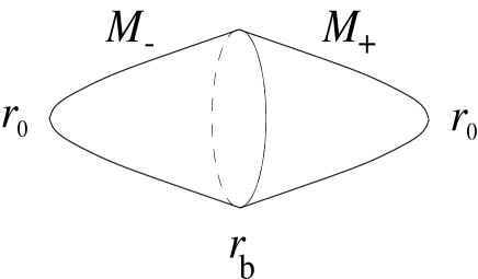
Figure 1: An embedding of the bulk ($r,\theta$) dimensions of ${\cal M}$ into $\mathbb{R}^{3}$.

The field equations (2)–(4) are modified by terms arising from the variation of the action (14), but can still be satisfied by appropriate junction conditions, according to the standard thin–shell formalism. In particular, the modification to the Einstein equation (2) is satisfied provided the discontinuity in the extrinsic curvature,$K_{ij}={h_{i}}^{k}\,{h_{j}}^{\ell}\,\nabla_{k}n_{\ell}$ is related to the 4–brane energy–momentum, $S_{ij}$, according to

$$[[K_{ij}]]=-2\kappa^{2}\left(S_{ij}-{1\over 4}S\;h_{ij}\right).$$ (17)

Here $[[X]]$ denotes the discontinuity in $X$ across the brane. The modified scalar equation is satisfied provided that the boundary term arising from the discontinuity in the derivative of $\phi$ cancels the variation of (14) w.r.t. $\phi$, leading to

$$\left[-{\textstyle{1\over 2}}\sqrt{-g}\,n^{\mu}\partial_{\mu}\phi+{\lambda T\over\kappa}\sqrt{-h}\,{\rm e}^{-\lambda\kappa\phi}\right]_{{r_{\lower 2.0pt\hbox{$\scriptscriptstyle b$}}}}=0\,.$$ (18)

The $U(1)$ gauge field strength, $F_{ab}$, can be chosen to be continuous at the junction, so that the Maxwell–type equation (3) is automatically satisfied. As observed in [11] it should be also possible to choose a gluing which would change the sign of $F_{ab}$ across the junction at the expense of adding a further “cosmological current” action term to the brane in addition to (14). Such a term would now involve a coupling to the scalar field, and would therefore modify the analysis that follows. We will not pursue that option here.

On account of (10) the solution to (18) is

$$T=\lambda^{-1}{r_{\lower 2.0pt\hbox{$\scriptstyle b$}}}^{2\lambda-1}\,.$$ (19)

This reduces the three unknown parameters, $T,\lambda,{r_{\lower 2.0pt\hbox{$\scriptstyle b$}}}$, to two independent ones. Further restrictions result from (17). For a static brane in Gaussian normal coordinates, $K_{ij}={\textstyle{1\over 2}}{\partial h_{ij}\over\partial\eta}$. Furthermore, while $\eta$ does not change sign across the brane, the direction of $r$ changes sign across the brane as $r$ points from ${r_{\lower 2.0pt\hbox{$\!\scriptstyle-$}}}$ to ${r_{\lower 2.0pt\hbox{$\scriptstyle b$}}}$, or ${r_{\lower 2.0pt\hbox{$\scriptstyle b$}}}$ to ${r_{\lower 2.0pt\hbox{$\scriptstyle+$}}}$, depending on whether the bolt is at ${r_{\lower 2.0pt\hbox{$\!\scriptstyle-$}}}$ or ${r_{\lower 2.0pt\hbox{$\scriptstyle+$}}}$. Thus

$$\epsilon\left({\rm d}r\over{\rm d}\eta\right)^{(-)}=-\epsilon\left({\rm d}r\over{\rm d}\eta\right)^{(+)}={\sqrt{\Delta}\over r}$$ (20)

where $\epsilon=\textrm{sign}(r_{\lower 2.0pt\hbox{$\scriptstyle b$}}-r_{\lower 2.0pt\hbox{$\scriptstyle 0$}})$, and the superscripts $(\pm)$ refer to the two sides of the 4–brane and are not to be confused with $r_{\lower 2.0pt\hbox{$\scriptstyle\pm$}}$. Hence the jump in the extrinsic curvature is

$$[[K_{ij}]]=-\epsilon{\sqrt{\Delta}\over r}{\partial h_{ij}\over\partial r}\bigg{|}_{r={r_{\lower 2.0pt\hbox{$\scriptscriptstyle b$}}}}={-T\over 2}\,{\rm e}^{-\lambda\kappa\phi}\,h_{ij}\,,$$ (21)

where we have also used $S_{ij}=-{\textstyle{T\over\kappa^{2}}}\,{\rm e}^{-\lambda\kappa\phi}h_{ij}$. Using (15) to substitute for the induced metric, eq. (21) reduces to the pair of equations

$$\partial_{r}\Delta({r_{\lower 2.0pt\hbox{$\scriptstyle b$}}}) = \displaystyle{\epsilon T\over 2}\,{r_{\lower 2.0pt\hbox{$\scriptstyle b$}}}\sqrt{\Delta({r_{\lower 2.0pt\hbox{$\scriptstyle b$}}})}\,{\rm e}^{-\lambda\kappa\phi({r_{\lower 2.0pt\hbox{$\scriptscriptstyle b$}}})}$$ (22)

$$\sqrt{\Delta({r_{\lower 2.0pt\hbox{$\scriptstyle b$}}})} = \displaystyle{\epsilon T\over 4}\,{r_{\lower 2.0pt\hbox{$\scriptstyle b$}}}^{2}\,{\rm e}^{-\lambda\kappa\phi({r_{\lower 2.0pt\hbox{$\scriptscriptstyle b$}}})}$$ (23)

or equivalently

$${\partial\over\partial r}\left({\Delta\over r^{2}}\right)\bigg{|}_{{r_{\lower 2.0pt\hbox{$\scriptscriptstyle b$}}}}=0\,.$$ (24)

Solving (24) we find

$${r_{\lower 2.0pt\hbox{$\scriptstyle b$}}}^{4}={2{B^{2}}\over A}={2{r_{\lower 2.0pt\hbox{$\scriptstyle+$}}}^{4}{r_{\lower 2.0pt\hbox{$\!\scriptstyle-$}}}^{4}\over{r_{\lower 2.0pt\hbox{$\scriptstyle+$}}}^{4}+{r_{\lower 2.0pt\hbox{$\!\scriptstyle-$}}}^{4}}.$$ (25)

We note that the brane position does not depend on the value of the scalar potential $\Lambda$. Combining (10), (19) and (23) we find

$$\lambda={\epsilon\over 4}{{r_{\lower 2.0pt\hbox{$\scriptstyle b$}}}\over\sqrt{\Delta({r_{\lower 2.0pt\hbox{$\scriptstyle b$}}})}}\,,$$ (26)

and

$$T=4\epsilon\sqrt{\Delta({r_{\lower 2.0pt\hbox{$\scriptstyle b$}}})}\,{r_{\lower 2.0pt\hbox{$\scriptstyle b$}}}^{\left({\textstyle{\epsilon{r_{\lower 2.0pt\hbox{$\scriptscriptstyle b$}}}\over 2\sqrt{\Delta({r_{\lower 2.0pt\hbox{$\scriptscriptstyle b$}}})}}}-2\right)},$$ (27)

where ${r_{\lower 2.0pt\hbox{$\scriptstyle b$}}}$ is given by (25) and $\Delta({r_{\lower 2.0pt\hbox{$\scriptstyle b$}}})$ by

$$\Delta({r_{\lower 2.0pt\hbox{$\scriptstyle b$}}})=\left(A\over 2\right)^{3/2}{1\over B}\left(1-{B^{2}\Lambda\over 2A}\right)\,,$$ (28)

in terms of $A$, $B$ and $\Lambda$. The tension is positive if we choose the bolt to be at $r_{\lower 2.0pt\hbox{$\scriptstyle 0$}}={r_{\lower 2.0pt\hbox{$\!\scriptstyle-$}}}$ so that $\epsilon=1$. We will avoid any potential problems associated with negative tension branes by henceforth choosing the bolt to be at ${r_{\lower 2.0pt\hbox{$\!\scriptstyle-$}}}$.

3.1 Consistency conditions when adding a thin-brane

It is possible to consider models without the restrictions which we have chosen to place on our parameters so that we could solve the bulk field equations. If we remove the restrictions we placed on $f,\bar{\lambda},\phi$ then we may consider what would be required of the parameters in the bulk to leave the field equations consistent upon addition of a thin brane at a finite distance from the fluxbrane, without explicitly solving Einstein’s equations for the bulk or junction conditions. Even solving the Einstein equations is difficult in the general case, although we present arguments in Appendix A that a class of solutions does exist in phenomenologically interesting cases, such as a positive cosmological constant, $\bar{\lambda}>0$, on the brane.

Consistency conditions of the form given in [10] can be used to further restrict the parameters of the model. Putting $D=6$, $p=3$ and $q=4$ in equation (2.17) of [10] and integrating over the boundary of the internal space we get

$$0 = \oint{\rm d}r\,{\rm d}\theta\;r^{\alpha+2}\Bigg{(}\alpha\bar{\cal R}r^{-2}+(3-\alpha)\tilde{\cal R}-(\alpha+3)\Lambda_{\rm Bulk}$$ (29)

$$-\kappa^{2}\bigg{[}(9-\alpha){T\over\kappa^{2}}\,{\rm e}^{-\lambda\kappa\phi}\delta(r-{r_{\lower 2.0pt\hbox{$\scriptstyle b$}}})-(3-\alpha){\cal T}^{\mu}_{\mu}-3(\alpha-1){\cal T}^{m}_{m}\bigg{]}\Bigg{)}.$$

Equations (5) and (6) give

$$\bar{\cal R} = 12\bar{\lambda}\,,$$ (30)

$$\tilde{\cal R} = {\partial_{r}f\partial_{r}\Delta-f\partial_{r}\partial_{r}\Delta\over f^{3}}\,,$$ (31)

and from (7)

$${\cal T}^{\mu}_{\mu} = {8B^{2}\over\kappa^{2}r^{10}f^{2}}{\rm e}^{\kappa\phi}-{(\partial_{r}\phi)^{2}\Delta\over f^{2}}-{2\over\kappa^{2}}\Lambda{\rm e}^{\kappa\phi}\,,$$ (32)

$${\cal T}^{m}_{m} = {\rm e}^{\kappa\phi}{4B^{2}\over\kappa^{2}r^{10}f^{2}}-{\rm e}^{\kappa\phi}{\Lambda\over\kappa^{2}}\,.$$ (33)

Putting $\alpha=3$ and $\Lambda_{\rm Bulk}=0$ in (29) this becomes

$$0=\oint{\rm d}r\,{\rm d}\theta\;r^{5}\left({36\bar{\lambda}\over r^{2}}-6T\,{\rm e}^{-\lambda\kappa\phi}\delta(r-{r_{\lower 2.0pt\hbox{$\scriptstyle b$}}})+{24B^{2}{\rm e}^{\kappa\phi}\over r^{10}f^{2}}-6\Lambda{\rm e}^{\kappa\phi}\right)$$ (34)

By examining the signs of the various terms we can find the parameter restrictions given in Table 1.

	$\Lambda<0$	$\Lambda=0$	$\Lambda>0$
$\vphantom{\vbox to14.0pt{\vfil}}\bar{\lambda}<0$	none	$B\neq 0$ or $T<0$	$B\neq 0$ or $T<0$
$\bar{\lambda}=0$	$T>0$	$T>0$ and $B\neq 0$	$B\neq 0$ or $T<0$
$\bar{\lambda}>0$	$T>0$	$T>0$	none

Table 1: Restrictions on $B$ and the sign of $T$ for given $\bar{\lambda}$ and $\Lambda$.

Some further small restrictions on the value of $B$ may result from the junction conditions once the function $\Delta(r)$ is specified for a particular geometry, as occurs in the analogous case of ref. [11]. However, as we are only able to specify an exact $\Delta(r)$ in the $\bar{\lambda}=0$ case (11), and not in the general case $\bar{\lambda}\neq 0$ case, we have not considered these additional restrictions in Table 1.

3.2 Further extensions of hybrid compactifications

One important question which is beyond the scope of our present analysis is the issue of how the inclusion of extra metric degrees of freedom, $\left\{{}^{6}\!g_{\mu\theta},{}^{6}\!g_{r\theta}\right\}$, in addition to the metric components (5) in six dimensions, would manifest themselves in the 4–dimensional effective theory. In the 5–dimensional Randall–Sundrum scenario [5, 6] standard model gauge fields are included by adding sources which are confined to the brane, as distributional terms in the 5–dimensional action.

In the present model, the situation is different since the $\theta$ coordinate is understood to parameterise a regular Kaluza–Klein type direction in the 6–dimensional theory. Thus it would appear we have the freedom to multiply the existing terms in (5) by appropriate functions of a new 5–dimensional scalar field, $\psi(x^{\mu},r)$, and to interpret additional non–zero components $\left\{{}^{6}\!g_{\mu\theta}(x^{\mu},r),{}^{6}\!g_{r\theta}(x^{\mu},r)\right\}$ of the metric in terms of functions of $\psi$ multiplied by a 5–dimensional $U(1)$ gauge potential. In this way, one would obtain a dimensional reduction from six to five dimensions similar to a standard Kaluza–Klein reduction of the Einstein–Hilbert action, but which is greatly complicated by the additional non-zero matter fields of the action (1) which contribute to the fluxbrane background. Addition of the thin brane, to achieve the final reduction to four dimensions, would then necessitate the addition of further terms to (14) to satisfy the junction conditions.

The extension of the model in this fashion is of considerable phenomenological interest, since we have the possibility not only of obtaining a massless graviton, but also a massless photon as an analogue of the Randall–Sundrum mode, together with a tower of very massive states. Given the considerable amount of work involved, we will not study the question of the existence of a massless $U(1)$ mode in four dimensions in the present paper, nor will we calculate mass gaps for the scalar, vector and tensor sectors. These questions are left to future work. Our primary interest in the present paper is to check that an appropriate graviton zero mode exists, with phenomenologically realistic corrections to Newton’s law, for parameter values which at the same time allow a solution of the hierarchy problem. To this end we will now solve an analogous problem for the static potential of a massless scalar field, and exhibit a non-linear gravitational wave solution with spectral properties equivalent to the massless scalar.

4 Static potential of the massless scalar field

The phenomenologically important derivation of the Newtonian limit and corrections should ideally be conducted in the context of a full tensorial perturbation analysis about the background solution. However, as was observed by Giddings, Katz and Randall [37] in the case of the Randall Sundrum model, if one is just interested in the static potential the relevant scalar gravitational mode shares the essential features with the static potential of a massless scalar field on the background. This approach was adopted in [11]. In this section we will perform a similar analysis for the background geometry described by eqs. (5)-(11) in the case that $\bar{g}_{\mu\nu}=\eta_{\mu\nu}$.

4.1 Scalar propagator

Our calculation will closely follow that of section $5$ of ref. [11]. We will add a massless minimally coupled scalar field, $\Phi$, to the model, with action

$$S_{\Phi}=-{\textstyle{1\over 2}}\int_{{\cal M}_{-}}{\rm d}^{6}x\,\sqrt{-g}\,(\nabla_{a}\Phi)(\nabla^{a}\Phi)\,.$$ (35)

on ${\cal M}_{-}$. This additional field $\Phi$ should not be confused with the scalar field, $\phi$, of the Salam-Sezgin model (1). We will calculate the static potential of a scalar field, $\Phi$, between two points on the thin brane with fixed $\theta$.

Rather than continuing with the coordinate basis of (5) it is convenient to introduce a new radial coordinate $\rho$ by

$$\rho={r^{4}-{r_{\lower 2.0pt\hbox{$\!\scriptstyle-$}}}^{4}\over{r_{\lower 2.0pt\hbox{$\scriptstyle+$}}}^{4}-r^{4}}\,,$$ (36)

which maps the interval ${r_{\lower 2.0pt\hbox{$\!\scriptstyle-$}}}<r<{r_{\lower 2.0pt\hbox{$\scriptstyle b$}}}$ to the interval $0<\rho<{\rho_{\lower 2.0pt\hbox{$\scriptstyle b$}}}$, where

$${\rho_{\lower 2.0pt\hbox{$\scriptstyle b$}}}=\left({{r_{\lower 2.0pt\hbox{$\!\scriptstyle-$}}}\over{r_{\lower 2.0pt\hbox{$\scriptstyle+$}}}}\right)^{4}\,,$$ (37)

is the position of the brane. In terms of the new radial coordinate $\rho$ the metric (5) becomes,

$${{\rm d}s_{\lower 2.0pt\hbox{$\scriptstyle 6$}}}^{2}=r^{2}\bar{g}_{\mu\nu}{\rm d}x^{\mu}{\rm d}x^{\nu}+{r^{2}\rho^{-1}\,{\rm d}\rho^{2}+\gamma^{2}r^{-6}\rho\,{\rm d}\theta^{2}\over 2\Lambda\left(1+\rho\right)^{2}}\,,$$ (38)

where by inverting (36)

$$r^{2}=\sqrt{{r_{\lower 2.0pt\hbox{$\!\scriptstyle-$}}}^{4}+{r_{\lower 2.0pt\hbox{$\scriptstyle+$}}}^{4}\rho\over 1+\rho}\,,$$ (39)

and the constant $\gamma$ is defined by

$$\gamma={\Lambda\over 2}({r_{\lower 2.0pt\hbox{$\scriptstyle+$}}}^{4}-{r_{\lower 2.0pt\hbox{$\!\scriptstyle-$}}}^{4})=4A\sqrt{1-{\Lambda B^{2}\over 2A^{2}}}\,.$$ (40)

We shall only be interested in the case of a flat lower–dimensional metric, $\bar{g}_{\mu\nu}=\eta_{\mu\nu}$, in what follows.

The scalar Green’s function, $G_{\lower 2.0pt\hbox{$\scriptstyle\Phi$}}$, is determined by the solution of the massless Klein-Gordon equation,

$$\nabla_{a}\nabla^{a}G_{\lower 2.0pt\hbox{$\scriptstyle\Phi$}}={1\over\sqrt{-g}}\partial_{a}(\sqrt{-g}g^{ab}\partial_{b}G_{\lower 2.0pt\hbox{$\scriptstyle\Phi$}})={\delta(\rho-\rho^{\prime})\delta(\theta-\theta^{\prime})\delta^{4}(x-x^{\prime})\over\sqrt{-g}}\,.$$ (41)

To simplify this problem we make the Fourier decomposition

$$G_{\lower 2.0pt\hbox{$\scriptstyle\Phi$}}(x,\rho,\phi;x^{\prime},\rho^{\prime},\phi^{\prime})=\int{{\rm d}^{4}k\over{(2\pi)}^{5}}{\rm e}^{ik_{\mu}(x^{\mu}-{x^{\prime}}\vphantom{\scriptstyle x}^{\mu})}\;\sum_{n=-\infty}^{\infty}{\rm e}^{in(\theta-\theta^{\prime})}G_{k,n}(\rho,\rho^{\prime})$$ (42)

where the indices of $k_{\mu}$ are raised and lowered by $\eta_{\mu\nu}$. We substitute (42) in (41) to obtain

$$\left\{\partial_{\rho}\left(\rho\partial_{\rho}\right)+{q^{2}\over 2\Lambda\left(1+\rho\right)^{2}}-{n^{2}\over\rho}\left(\beta+{2\rho\over\Lambda(1+\rho)}\right)^{2}\right\}G_{k,n}(\rho,\rho^{\prime})={\delta(\rho-\rho^{\prime})\over\gamma}\,.$$ (43)

where $q^{2}=-k_{\mu}k^{\mu}=k_{0}^{2}-\mathbf{k}^{2}$, and the constant $\beta$ is defined by

$$\beta={{r_{\lower 2.0pt\hbox{$\!\scriptstyle-$}}}^{4}\over\gamma}={2{\rho_{\lower 2.0pt\hbox{$\scriptstyle b$}}}\over\Lambda(1-{\rho_{\lower 2.0pt\hbox{$\scriptstyle b$}}})}\,.$$ (44)

When $\rho\neq\rho^{\prime}$ (43) is a Sturm-Liouville equation, with the general solution

$$G_{k,n}=C_{n}X_{n}(\rho)+D_{n}Y_{n}(\rho),$$ (45)

where $C_{n}$ and $D_{n}$ are constants and for $n=0$,

$$X_{\lower 2.0pt\hbox{$\scriptstyle 0$}}=\sqrt{2\over\gamma}\,{\cal P}_{\nu-1}\left(1-\rho\over 1+\rho\right),\qquad Y_{\lower 2.0pt\hbox{$\scriptstyle 0$}}=\sqrt{2\over\gamma}\,{\cal Q}_{\nu-1}\left(1-\rho\over 1+\rho\right),$$ (46)

${\cal P}$ and ${\cal Q}$ being Legendre functions of the first and second kind respectively, while for $n\neq 0$,

$$X_{n} = {\rho^{n\beta}\left(1+\rho\right)^{1-\nu}\over\sqrt{2n\beta\gamma}}\;{}_{2}{\cal F}_{1}\left(\left[{1-\nu+{2n\over\Lambda}+2n\beta},{1-\nu-{2n\over\Lambda}}\right];{1+2n\beta};{-\rho}\right)\,,$$ (47)

$$= {\rho^{n\beta}\left(1+\rho\right)^{2n/\Lambda}\over\sqrt{2n\beta\gamma}}\;{}_{2}{\cal F}_{1}\left(\left[{\nu-{2n\over\Lambda}},{1-\nu-{2n\over\Lambda}}\right];{1+2n\beta};{\rho\over 1+\rho}\right)\,,$$

and

$$Y_{n} = {\left(1+\rho\right)^{1-\nu}\over\sqrt{2n\beta\gamma}\,\rho^{n\beta}}\;{}_{2}{\cal F}_{1}\left(\left[{1-\nu+{2n\over\Lambda}},{1-\nu-{2n\over\Lambda}-2n\beta}\right];{1-2n\beta};{-\rho}\right)\,,$$

$$= {\left(1+\rho\right)^{2n(\beta+1/\Lambda)}\over\sqrt{2n\beta\gamma}\,\rho^{n\beta}}\;{}_{2}{\cal F}_{1}\left(\left[{\nu-{2n\over\Lambda}-2n\beta},{1-\nu-{2n\over\Lambda}-2n\beta}\right];{1-2n\beta};{\rho\over 1+\rho}\right)\,,$$

where ${}_{2}{\cal F}_{1}$ is a standard hypergeometric function [42], and for all values of $n$, including $n=0$,

$$\nu\equiv{\textstyle{1\over 2}}\left(1+\sqrt{1+{2q^{2}\over\Lambda}+{16n^{2}\over\Lambda^{2}}}\,\right)\,.$$ (49)

For $n\neq 0$, as $\rho\to 0$, the leading two terms in the series expansions for $X_{n}(\rho)$ and $Y_{n}(\rho)$ match those of Bessel functions, $J_{\pm 2n\beta}$, or modified Bessel functions, $I_{\pm 2n\beta}$ in the argument $\left|{2\over\Lambda}(8n^{2}\beta-q^{2})\rho\right|^{1/2}$ up to an overall constant of proportionality:

$$X_{n}(\rho) = {\rho^{n\beta}\over\sqrt{2n\beta}}\left[1+{8n^{2}\beta-q^{2}\over 2\Lambda(1+2n\beta)}\rho+{\mathrm{O}}(\rho^{2})\right]$$ (50)

$$\propto {\cases{J_{2n\beta}\left(\sqrt{{2\over\Lambda}(q^{2}-8n^{2}\beta)\rho}\,\right)+{\mathrm{O}}(\rho^{2+n\beta}),&$n^{2}<q^{2}/(8\beta)$\cr I_{2n\beta}\left(\sqrt{{2\over\Lambda}(8n^{2}\beta-q^{2})\rho}\,\right)+{\mathrm{O}}(\rho^{2+n\beta}),&$n^{2}>q^{2}/(8\beta)$\cr}}\ ,$$

and

$$Y_{n}(\rho) = {\rho^{-n\beta}\over\sqrt{2n\beta}}\left[1+{8n^{2}\beta-q^{2}\over 2\Lambda(1-2n\beta)}\rho+{\mathrm{O}}(\rho^{2})\right]$$ (51)

$$\propto {\cases{J_{-2n\beta}\left(\sqrt{{2\over\Lambda}(q^{2}-8n^{2}\beta)\rho}\,\right)+{\mathrm{O}}(\rho^{2-n\beta}),&$n^{2}<q^{2}/(8\beta)$\cr I_{-2n\beta}\left(\sqrt{{2\over\Lambda}(8n^{2}\beta-q^{2})\rho}\,\right)+{\mathrm{O}}(\rho^{2-n\beta}),&$n^{2}>q^{2}/(8\beta)$\cr}}\ .$$

Using (46), (50) and (51) the Wronskian of the linearly independent solutions satisfies

$${\cal W}\left[X_{n}(\rho),Y_{n}(\rho)\right]\equiv X_{n}\partial_{\rho}Y_{n}-Y_{n}\partial_{\rho}X_{n}={-1\over\gamma\rho}\,.$$ (52)

The overall coefficients in (46), (47) and (LABEL:Yhyp) were chosen to make the r.h.s. of (52) independent of $n$.

4.2 Boundary and matching conditions

We now wish to solve the inhomogeneous version of (43). Without loss of generality, we pick the brane to be to a distance $\xi={\rho_{\lower 2.0pt\hbox{$\scriptstyle b$}}}-\rho^{\prime}>0$ to the right of the discontinuity. We will later let $\xi\to 0$ so that the brane explicitly becomes the source of the discontinuity. We have general solutions to the left and right of the discontinuity at $\rho=\rho^{\prime}$, labelled

$$G_{k,n}=\cases{G_{\lower 2.0pt\hbox{$\scriptstyle<$}}(\rho,\rho^{\prime})=A_{\lower 2.0pt\hbox{$\scriptstyle 1$}}(\rho^{\prime})X_{n}(\rho)+A_{\lower 2.0pt\hbox{$\scriptstyle 2$}}(\rho^{\prime})Y_{n}(\rho),&$\rho<\rho^{\prime}$,\cr G_{\lower 2.0pt\hbox{$\scriptstyle>$}}(\rho,\rho^{\prime})=B_{\lower 2.0pt\hbox{$\scriptstyle 1$}}(\rho^{\prime})X_{n}(\rho)+B_{\lower 2.0pt\hbox{$\scriptstyle 2$}}(\rho^{\prime})Y_{n}(\rho),&$\rho>\rho^{\prime}$,\cr}$$ (53)

We will assume that $G_{k,n}(\rho,\rho^{\prime})$ is finite at $\rho=0$, and adopt a Neumann boundary condition at the brane $\rho={\rho_{\lower 2.0pt\hbox{$\scriptstyle b$}}}$,

$$\partial_{\rho}G_{k,n}|_{\lower 2.0pt\hbox{$\scriptstyle\rho={\rho_{\lower 2.0pt\hbox{$\scriptscriptstyle b$}}}$}}=0\,.$$ (54)

Imposition of regularity of the solution as $\rho\to 0$ excludes $Y_{n}$ as a solution, leading to the choice $A_{2}(\rho^{\prime})=0$. Furthermore, (54) applied to $G_{\lower 2.0pt\hbox{$\scriptstyle>$}}(\rho,\rho^{\prime})$ implies

$${B_{2}(\rho^{\prime})\over B_{1}(\rho^{\prime})}=-{X_{n},_{b}\over Y_{n},_{b}}\,.$$ (55)

where

$$X_{n},_{b}\equiv\left.\partial_{\rho}X_{n}\right|_{\lower 2.0pt\hbox{$\scriptstyle\rho={\rho_{\lower 2.0pt\hbox{$\scriptscriptstyle b$}}}$}},\qquad X_{n},_{b}\equiv\left.\partial_{\rho}Y_{n}\right|_{\lower 2.0pt\hbox{$\scriptstyle\rho={\rho_{\lower 2.0pt\hbox{$\scriptscriptstyle b$}}}$}}.$$ (56)

The matching conditions at $\rho=\rho^{\prime}$ are

$$\left.\left(G_{\lower 2.0pt\hbox{$\scriptstyle<$}}-G_{\lower 2.0pt\hbox{$\scriptstyle>$}}\right)\right|_{\lower 2.0pt\hbox{$\scriptstyle\rho=\rho^{\prime}$}} = 0\,,$$ (57)

$$\left.\partial_{\rho}\left(G_{\lower 2.0pt\hbox{$\scriptstyle>$}}-G_{\lower 2.0pt\hbox{$\scriptstyle<$}}\right)\right|_{\lower 2.0pt\hbox{$\scriptstyle\rho=\rho^{\prime}$}} = {1\over\gamma\rho^{\prime}}\,.$$ (58)

Combining the boundary conditions, the matching conditions and (52) we find the solution of the boundary value problem,

$$G_{k,n}(\rho,\rho^{\prime})=\cases{G_{\lower 2.0pt\hbox{$\scriptstyle<$}}(\rho,\rho^{\prime})=\displaystyle{X_{n}(\rho)\over X_{n},_{b}}\left(X_{n}(\rho^{\prime})Y_{n},_{b}-Y_{n}(\rho^{\prime})X_{n},_{b}\right),&$\rho<\rho^{\prime}$,\cr G_{\lower 2.0pt\hbox{$\scriptstyle>$}}(\rho,\rho^{\prime})=\displaystyle{X_{n}(\rho^{\prime})\over X_{n},_{b}}\left(X_{n}(\rho)Y_{n},_{b}-Y_{n}(\rho)X_{n},_{b}\right),&$\rho>\rho^{\prime}$.\cr}$$ (59)

The scalar Green’s function, $G_{\lower 2.0pt\hbox{$\scriptstyle\Phi$}}$, is now determined by substituting (59) into (42) and prescribing the integration as desired at the poles, which in this case correspond to the zeroes of $X_{n},_{b}$.

4.3 Static potential on the brane

Given the brane is the source of the discontinuity for the Green’s function, we set $\rho^{\prime}=\rho_{b}$ by letting $\xi\to 0$. With $\rho={\rho_{\lower 2.0pt\hbox{$\scriptstyle b$}}}$, and using (52), the Green’s function (59) reduces to

$$G_{k,n}({\rho_{\lower 2.0pt\hbox{$\scriptstyle b$}}})=-{X_{n}({\rho_{\lower 2.0pt\hbox{$\scriptstyle b$}}})\over\gamma{\rho_{\lower 2.0pt\hbox{$\scriptstyle b$}}}X_{n},_{b}}\,.$$ (60)

To obtain the static potential, we explicitly integrate the retarded Green’s function (42), (60) over the time difference, $t-t^{\prime}$. We note that $G_{\lower 2.0pt\hbox{$\scriptstyle\Phi$}}$ is non-zero only for $t-t^{\prime}>0$, so multiplying it by $\theta(t-t^{\prime})$ leaves it unchanged. We can then perform the integration over $t$ to find

$$V_{\Phi}(\mathbf{x},\phi;\mathbf{x}^{\prime},\phi^{\prime})=-\sum_{n=-\infty}^{\infty}{\rm e}^{in(\theta-\theta^{\prime})}\int{{\rm d}^{3}\mathbf{k}\over(2\pi)^{5}}\,{\rm e}^{i\mathbf{k}\cdot(\mathbf{x}-\mathbf{x}^{\prime})}\int_{-\infty}^{\infty}{{\rm d}k^{0}\over i(k^{0}-i\epsilon)}{X_{n}({\rho_{\lower 2.0pt\hbox{$\scriptstyle b$}}})\over\gamma{\rho_{\lower 2.0pt\hbox{$\scriptstyle b$}}}X_{n},_{b}},$$ (61)

We are interested in the retarded Green’s function, which requires that we perform the $k^{0}$ integral by a contour integration with $q^{2}\to(k^{0}+i\epsilon)^{2}-{\bf k}^{2}$, $\epsilon\to 0_{+}$. We close the contour in the upper half plane, to avoid the poles which correspond to the zeroes of $X_{n},_{b}$ on the real line, and which are moved below the real line by the $\epsilon$–procedure. The only residue is then due to the simple pole at $k^{0}=0$, and the integration yields

$$V_{\Phi}(\mathbf{x},\phi;\mathbf{x}^{\prime},\phi^{\prime}) = -\sum_{n=-\infty}^{\infty}{\rm e}^{in(\theta-\theta^{\prime})}\int{{\rm d}^{3}\mathbf{k}\over(2\pi)^{4}}\,{\rm e}^{i\mathbf{k}\cdot(\mathbf{x}-\mathbf{x}^{\prime})}\,{\cal G}_{n}(-k^{2}),$$ (62)

$$= -\sum_{n=-\infty}^{\infty}{\rm e}^{in(\theta-\theta^{\prime})}\int_{0}^{\infty}{{\rm d}k\over 4\pi^{3}}\,{k\sin(k|\mathbf{x}-\mathbf{x}^{\prime}|)\over|\mathbf{x}-\mathbf{x}^{\prime}|}\,{\cal G}_{n}(-k^{2})\,,$$

$$= -\sum_{n=-\infty}^{\infty}{\rm e}^{in(\theta-\theta^{\prime})}\hbox{Im}\;\left(\int_{-\infty}^{\infty}{{\rm d}k\over 8\pi^{3}}{k\,{\rm e}^{ik|\mathbf{x}-\mathbf{x}^{\prime}|}\over|\mathbf{x}-\mathbf{x}^{\prime}|}\,{\cal G}_{n}(-k^{2})\right)\,,$$

where $k=|\mathbf{k}|$, and ${\cal G}_{n}(-k^{2})\equiv\left.G_{k,n}({\rho_{\lower 2.0pt\hbox{$\scriptstyle b$}}})\right|_{q^{2}=-\mathbf{k}^{2}}$.

The final integral in (62) can be performed by a careful choice of contour, subject to convergence of the integrand, which we have checked numerically. It is found that for $n=0$, ${\cal G}_{\lower 2.0pt\hbox{$\scriptstyle 0$}}(-k^{2})$ has a second order pole at $k=0$, together with first order poles at $k=\pm iq_{\lower 2.0pt\hbox{$\scriptstyle 0,j$}}$, where $q_{\lower 2.0pt\hbox{$\scriptstyle 0,j$}}>0$, $j=1,\dots,\infty$. For $n\neq 0$, all poles occur at $k=\pm iq_{\lower 2.0pt\hbox{$\scriptstyle n,j$}}$, where $q_{\lower 2.0pt\hbox{$\scriptstyle n,j$}}>0$, $j=1,\dots,\infty$. We close the contour in the upper half plane, but perform a cut on the Im$(k)$ axis on the interval $k\in({\textstyle{1\over 2}}i\bar{q},\infty)$, where $\bar{q}=\;\hbox{inf}\;\{q_{n,j}|j=1,\dots,\infty\}$. Integrating back and forth around the cut, first from $k=\epsilon+i\infty$ to $k=\epsilon+{\textstyle{1\over 2}}i\bar{q}$ in the Re$(k)>0$ quadrant and then back from $k=-\epsilon+{\textstyle{1\over 2}}i\bar{q}$ to $k=-\epsilon+i\infty$ in the Re$(k)<0$ quadrant before taking the limit $\epsilon\to 0$, has the net effect of circumscribing each of the poles on the positive imaginary axis once in a clockwise fashion.

We will not analytically determine each coefficient in the sum of terms in (62) which result from the enclosed poles at $k=iq_{\lower 2.0pt\hbox{$\scriptstyle n,j$}}$, but simply note that the Laurent expansion of ${\cal G}_{n}(-k^{2})$ at each of these poles takes the form

$${\cal G}_{n}(-k^{2})={C_{n,j}({\rho_{\lower 2.0pt\hbox{$\scriptstyle b$}}})\over k^{2}+q_{n,j}^{2}}+{\rm O}(1)\,,$$ (63)

in terms of coefficients $C_{n,j}({\rho_{\lower 2.0pt\hbox{$\scriptstyle b$}}})$, and the residue gives a Yukawa correction in each case.

The pole at $k=0$ is not enclosed by the contour, but since it lies on the contour, taking the principal part gives a net contribution to the static potential, which is readily determined analytically by applying identities which hold for the Legendre function solutions (46) for $n=0$. In particular,

$$\hbox{Res}\;\left(k\,{\rm e}^{ik|\mathbf{x}-\mathbf{x}^{\prime}|}{\cal G}_{\lower 2.0pt\hbox{$\scriptstyle 0$}}(-k^{2})\right)_{k=0} = \hbox{Res}\;\left(-k{\rm e}^{ik|\mathbf{x}-\mathbf{x}^{\prime}|}{\cal P}_{\nu-1}(y)\over{\textstyle{1\over 2}}\gamma(1-y^{2})\partial_{y}{\cal P}_{\nu-1}(y)\right)_{k=0,\rho={\rho_{\lower 2.0pt\hbox{$\scriptscriptstyle b$}}}}$$ (64)

$$= \hbox{Res}\;\left(-2k{\rm e}^{ik|\mathbf{x}-\mathbf{x}^{\prime}|}{\cal P}_{\nu-1}(y)\over\gamma\nu\left[y{\cal P}_{\nu-1}(y)-P_{\nu}(y)\right]\right)_{k=0,\rho={\rho_{\lower 2.0pt\hbox{$\scriptscriptstyle b$}}}}$$

$$= \lim_{\nu\to 1}\left.4\Lambda{\cal P}_{\nu-1}(y)\over\gamma\left[y\partial_{\nu}{\cal P}_{\nu-1}(y)-\partial_{\nu}P_{\nu}(y)\right]\right|_{\rho={\rho_{\lower 2.0pt\hbox{$\scriptscriptstyle b$}}}}$$

$$= {2\Lambda(1+{\rho_{\lower 2.0pt\hbox{$\scriptstyle b$}}})\over\gamma{\rho_{\lower 2.0pt\hbox{$\scriptstyle b$}}}}\,,$$

where in the intermediate steps $y$ is defined implicitly by $y=(1-\rho)/(1+\rho)$, and we have used the fact that as $k\to 0$, $\nu\simeq 1-k^{2}/(2\Lambda)$, ${\cal P}_{\lower 2.0pt\hbox{$\scriptstyle 0$}}(y)=1$, and the identities $\lim_{\nu\to 1}\partial_{\nu}{\cal P}_{\nu-1}(y)=\ln[{\textstyle{1\over 2}}(1+y)]$, and $\lim_{\nu\to 1}\partial_{\nu}{\cal P}_{\nu}(y)=y\ln[{\textstyle{1\over 2}}(1+y)]+y-1$.

The final expression for the static potential then becomes

$$V_{\Phi}(\mathbf{x},\phi;\mathbf{x}^{\prime},\phi^{\prime})={-(1+{\rho_{\lower 2.0pt\hbox{$\scriptstyle b$}}})\Lambda\over 4\pi^{2}\gamma{\rho_{\lower 2.0pt\hbox{$\scriptstyle b$}}}|\mathbf{x}-\mathbf{x}^{\prime}|}-\sum_{n=-\infty}^{\infty}\sum_{j=1}^{\infty}{C_{n,j}({\rho_{\lower 2.0pt\hbox{$\scriptstyle b$}}})e^{-q_{n,j}|\mathbf{x}-\mathbf{x}^{\prime}|}\over 8\pi^{2}|\mathbf{x}-\mathbf{x}^{\prime}|}\,.$$ (65)

which as expected is a Newtonian–type potential supplemented by Yukawa–type corrections. The constant $\gamma$ may be re-expressed in terms of ${r_{\lower 2.0pt\hbox{$\!\scriptstyle-$}}}$ and ${\rho_{\lower 2.0pt\hbox{$\scriptstyle b$}}}$ on account of (44).

4.4 Nonlinear gravitational waves on the brane

We will now further justify the claim that the calculation of the static potential for a minimally coupled massless scalar field given above reproduces all the essential features of the corresponding calculation for the graviton. We observe that the construction of nonlinear gravitational waves which was developed in ref. [11] by a generalization of the technique of Garfinkle and Vachaspati [38], is unchanged when applied to the background (5). In particular, nonlinear gravitational waves can be constructed on the background in the case that the geometry, ${\cal M}_{\rm low}$, generated by the 4–dimensional metric $\bar{g}_{\mu\nu}$ admits a hypersurface–orthogonal null Killing vector, $k^{\mu}$. If $\bar{z}$ is a locally defined scalar such that $\partial_{[\mu}k_{\nu]}=k_{[\nu}\partial_{\mu]}\bar{z}$ and $k^{\mu}\partial_{\mu}{z}=0$, where Greek indices are lowered and raised with $\bar{g}_{\mu\nu}$ and its inverse, then the nonlinear wave spacetime is given by adding to (5) the term

$$r^{2}H{\rm e}^{-{z}}k_{\mu}k_{\nu}{\rm d}x^{\mu}{\rm d}x^{\nu},$$ (66)

where ${z}$ is the pullback of $\bar{z}$ to (5), and $H$ is a scalar function on the bulk spacetime (5), which satisfies $\nabla^{a}\nabla_{a}H=0$, and $\ell^{a}\partial_{a}H=0$. Here $\nabla_{a}$ is the covariant derivative in the metric (5) and $\ell^{a}=(k^{\mu},0,0)$ is the extension of $k^{\mu}$ to (5), with indices raised and lowered by the full spacetime metric (5). The vector, $\ell^{a}$, is also null and hypersurface orthogonal, and satisfies $\partial_{[a}\ell_{b]}=\ell_{[b}\partial_{a]}({z}+2\ln r)$ and $\ell^{a}\partial_{a}({z}+2\ln r)=0$.

In addition to the junction conditions (18), (22)–(24), we now have the additional relation

$${\sqrt{\Delta({r_{\lower 2.0pt\hbox{$\scriptstyle b$}}})}\over{r_{\lower 2.0pt\hbox{$\scriptstyle b$}}}}\left.\partial_{r}(r^{2}H)\right|_{r_{\lower 2.0pt\hbox{$\scriptscriptstyle b$}}}=\displaystyle{\epsilon T\over 2}\,{\rm e}^{-\lambda\kappa\phi({r_{\lower 2.0pt\hbox{$\scriptscriptstyle b$}}})}{r_{\lower 2.0pt\hbox{$\scriptstyle b$}}}^{2}H({r_{\lower 2.0pt\hbox{$\scriptstyle b$}}})$$ (67)

Using (23) we see that (67) is equivalent to the Neumann condition

$$\left.\partial_{r}H\right|_{r_{\lower 2.0pt\hbox{$\scriptscriptstyle b$}}}=0,$$ (68)

at the brane, if $H$ is viewed as a massless scalar field on the spacetime without the term (66). In the case that $\bar{g}_{\mu\nu}=\eta_{\mu\nu}$ the field $H$ therefore satisfies the same wave equation and boundary conditions as were given above for massless scalar field, $\Phi$.

To make the correspondence explicit, we take $\bar{g}_{\mu\nu}=\eta_{\mu\nu}$, and adopt double null coordinates, $(u,v,x_{\perp}^{1},x_{\perp}^{2})$, on the Minkowski space, ${\cal M}_{\rm low}$. If we choose $k^{\mu}=(\partial_{v})^{\mu}$, the solution with the gravitational wave term (66) reads

$${\rm d}s^{2}=r^{2}\left[-{\rm d}u{\rm d}v+H(u,x_{\perp}^{k},r,\phi){\rm d}u^{2}+\delta_{\lower 2.0pt\hbox{$\scriptstyle AB$}}{\rm d}x_{\perp}^{A}{\rm d}x_{\perp}^{B}\right]+{r^{2}{\rm d}r^{2}\over\Delta}+\Delta{\rm d}\phi^{2}\,,$$ (69)

where $\Delta$ is given by (11). Note that $H$ does not depend on $v$ but its dependence on $u$ is arbitrary. The scalar wave equation for $H$ explicitly reads

$$H,_{rr}+\left({3\over r}+{\Delta,_{r}\over\Delta}\right)H,_{r}+{r^{2}H,_{\phi\phi}\over\Delta^{2}}+{\delta^{AB}H,_{AB}\over\Delta}=0.$$ (70)

The general linearized limit of the nonlinear gravitational solution can be discussed as in [44]. We note that $H=h_{AB}(u)x_{\perp}^{A}x_{\perp}^{B}$, where $h_{\lower 2.0pt\hbox{$\scriptstyle 22$}}(u)=-h_{\lower 2.0pt\hbox{$\scriptstyle 11$}}(u)$, is clearly a solution: it satisfies $\delta^{AB}H,_{AB}=0$, and its linearized limit is analogous to the famous normalizable massless mode in the Randall–Sundrum II model [6]. If we transform the radial parameter to $\rho$ by (36) and make a Fourier decomposition as in (42), then (70) becomes equivalent to the homogeneous part of (43). Our analysis above for the massless scalar field therefore applies equally to the graviton mode.

The nonlinear gravitational wave construction also applies firstly to any other Ricci–flat geometry on ${\cal M}_{\rm low}$ which admits a hypersurface orthogonal null Killing vector, and secondly with suitable modifications to other Einstein space geometries for ${\cal M}_{\rm low}$, provided appropriate solutions can be found.

5 The hierarchy problem

One of the principal motivations for studying brane world models is the attempt to provide a natural solution to the hierarchy problem between the Planck and electroweak scales. The construction of ref. [11] potentially offers a concrete realization of the phenomenological solution to the hierarchy problem proposed by Antoniadis [39], Arkani-Hamed, Dimopoulos and Dvali [40, 41]. In particular, if the non-gravitational forces can be introduced in such a way as to be confined to the brane, then provided that the distance between the thin brane and the bolt can be made large enough, higher–dimensional gravitational corrections could become manifest close to the TeV scale.

Since the construction is a hybrid one, there is an ordinary Kaluza–Klein direction within the 4–brane in addition to the direction transverse to the brane. A phenomenologically realistic solution to the hierarchy problem can therefore only be obtained if the distance between the brane and the bolt can be made many orders of magnitude larger than the circumference of the Kaluza–Klein circle. In the original construction of ref. [11], based on Einstein–Maxwell gravity with a higher–dimensional cosmological constant, a natural solution to the hierarchy problem proved to be impossible as the brane–bolt distance was at most comparable to the circumference of the Kaluza–Klein circle. The present model has more degrees of freedom, however, and so it is possible that this problem can be overcome.

In order to make the volume of the internal space, ${\cal V}$, sufficiently large to accommodate TeV scale gravity, we must be able to find a set of parameters $(A,B,\Lambda)$ which allows the ratio, $R={\cal V}/{\cal C}$, to be arbitrarily large. The proper circumference of the Kaluza–Klein direction is

$${\cal C}={4\pi\sqrt{\Delta({r_{\lower 2.0pt\hbox{$\scriptstyle b$}}})}\over\Delta^{\prime}({r_{\lower 2.0pt\hbox{$\!\scriptstyle-$}}})}={2^{3/4}\pi{\rho_{\lower 2.0pt\hbox{$\scriptstyle b$}}}^{1/2}\over\sqrt{\Lambda}\,\sqrt[4]{1+{\rho_{\lower 2.0pt\hbox{$\scriptstyle b$}}}}}\,.$$ (71)

The volume of the internal space, ${\cal V}=2\int_{r_{\lower 2.0pt\hbox{$\scriptscriptstyle\!-$}}}^{{r_{\lower 2.0pt\hbox{$\scriptscriptstyle b$}}}}\int_{\lower 2.0pt\hbox{$\scriptstyle 0$}}^{4\pi/\Delta^{\prime}(r_{\lower 2.0pt\hbox{$\scriptscriptstyle\!-$}})}{\rm d}\ell_{\theta}{\rm d}\ell_{r}$ is

$${\cal V}=({{r_{\lower 2.0pt\hbox{$\scriptstyle b$}}}}^{2}-{{r_{\lower 2.0pt\hbox{$\!\scriptstyle-$}}}}^{2}){4\pi\over\Delta^{\prime}({r_{\lower 2.0pt\hbox{$\!\scriptstyle-$}}})}$$ (72)

The ratio, $R={\cal V}/{\cal C}$ is then simply

$$R={({{r_{\lower 2.0pt\hbox{$\scriptstyle b$}}}}^{2}-{{r_{\lower 2.0pt\hbox{$\!\scriptstyle-$}}}}^{2})\over\sqrt{\Delta({r_{\lower 2.0pt\hbox{$\scriptstyle b$}}})}}=\sqrt{2\over\Lambda}\,{r_{\lower 2.0pt\hbox{$\!\scriptstyle-$}}}\,F({\rho_{\lower 2.0pt\hbox{$\scriptstyle b$}}})$$ (73)

where ${r_{\lower 2.0pt\hbox{$\!\scriptstyle-$}}}$ is given by (12),

$$F({\rho_{\lower 2.0pt\hbox{$\scriptstyle b$}}})={4{\rho_{\lower 2.0pt\hbox{$\scriptstyle b$}}}^{1/2}\over 1-{\rho_{\lower 2.0pt\hbox{$\scriptstyle b$}}}}\left(\sqrt{2\over 1+{\rho_{\lower 2.0pt\hbox{$\scriptstyle b$}}}}-1\right)\sqrt[4]{1+{\rho_{\lower 2.0pt\hbox{$\scriptstyle b$}}}\over 2}\,,$$ (74)

and on account of (12) and (37),

$${\rho_{\lower 2.0pt\hbox{$\scriptstyle b$}}}={A-\sqrt{A-{\textstyle{1\over 2}}B^{2}\Lambda}\over A+\sqrt{A-{\textstyle{1\over 2}}B^{2}\Lambda}}\,.$$ (75)

Figure 2: The ratio of volume of the internal space to its circumference is a multiple of $F({\rho_{\lower 2.0pt\hbox{$\scriptstyle b$}}})$, as given by (73), (74). It is plotted here versus ${\rho_{\lower 2.0pt\hbox{$\scriptstyle b$}}}^{1/4}$.

The quantity $F({\rho_{\lower 2.0pt\hbox{$\scriptstyle b$}}})$ defined by (74) is depicted in Fig. 2. It is a monotonic function which increases from $F=0$ to $F=1$ on the interval ${\rho_{\lower 2.0pt\hbox{$\scriptstyle b$}}}\in[0,1]$. The limit ${\rho_{\lower 2.0pt\hbox{$\scriptstyle b$}}}\to 1$ occurs when ${B^{2}\Lambda\over 2A^{2}}\to 1$, i.e., when ${r_{\lower 2.0pt\hbox{$\!\scriptstyle-$}}}\approx{r_{\lower 2.0pt\hbox{$\scriptstyle+$}}}\approx{r_{\lower 2.0pt\hbox{$\scriptstyle b$}}}\approx{4A\over\Lambda}$. In this case ${\cal C}\approx\sqrt{2}\pi\Lambda^{-1/2}$, and $R={\cal V}/{\cal C}\approx 2^{5/2}A\Lambda^{-3/2}$. The requirement that ${\cal C}$ must be small enough to be interpreted as a conventional Kaluza–Klein direction means that $\Lambda$ must be suitably large. Since the parameter $A$ is still free, however, we can still make $R$ arbitrarily large to overcome its dependence on the $\Lambda^{-3/2}$ factor. Thus it appears that a solution to the hierarchy problem may be feasible.

For smaller values of ${\rho_{\lower 2.0pt\hbox{$\scriptstyle b$}}}$ similar arguments apply. In particular, consider the extreme limit ${\rho_{\lower 2.0pt\hbox{$\scriptstyle b$}}}\to 0$ which corresponds to $0<{\textstyle{B^{2}\Lambda\over 2A^{2}}}\ll 1$. Then ${r_{\lower 2.0pt\hbox{$\!\scriptstyle-$}}}^{4}\approx B^{2}/A$, ${r_{\lower 2.0pt\hbox{$\scriptstyle+$}}}^{4}\approx 8A/\Lambda$ and $F({\rho_{\lower 2.0pt\hbox{$\scriptstyle b$}}})\approx 4(\sqrt{2}\,-1){\rho_{\lower 2.0pt\hbox{$\scriptstyle b$}}}^{1/2}$. Hence $R\approx 2(\sqrt{2}\,-1)B^{3/2}A^{-5/4}$ and ${\cal C}\approx 2^{-3/4}\pi BA^{-1}$, which are both independent of $\Lambda$. Since the constants $A$ and $B$ are not constrained except by the requirement ${\textstyle{B\over A}}\ll\sqrt{{\textstyle{2\over\Lambda}}}$, we can again make $R$ arbitrarily large while keeping ${\cal C}$ small. If we denote $R_{\lower 2.0pt\hbox{$\scriptstyle 0$}}$ and ${\cal C}_{\lower 2.0pt\hbox{$\scriptstyle 0$}}$ to be phenomenologically desirable values of $R$ and ${\cal C}$, we can conversely fix both $A$ and $B$. We find $A_{0}=\pi^{6}{R_{\lower 2.0pt\hbox{$\scriptstyle 0$}}}^{4}\,2^{-17/2}(\sqrt{2}\,-1)^{-4}{\cal C}_{\lower 2.0pt\hbox{$\scriptstyle 0$}}^{-6}$ and $B_{0}=\pi^{5}{R_{\lower 2.0pt\hbox{$\scriptstyle 0$}}}^{4}\,2^{-31/4}(\sqrt{2}\,-1)^{-4}{\cal C}_{\lower 2.0pt\hbox{$\scriptstyle 0$}}^{-5}$, while for consistency of the limit $0<\Lambda_{0}\ll{\textstyle{\pi^{2}\over\sqrt{2}{{\cal C}_{\lower 2.0pt\hbox{$\scriptscriptstyle 0$}}}^{2}}}$.

We have demonstrated here that a solution of the hierarchy problem is possible regardless of the value of ${\rho_{\lower 2.0pt\hbox{$\scriptstyle b$}}}$. We note, however, that once the Newton potential for the tensor modes, equivalent to the first term of (65), is determined then two of the parameters, $r_{-}$, $\Lambda$ and ${\rho_{\lower 2.0pt\hbox{$\scriptstyle b$}}}$ would be fixed phenomenologically via equations similar to (65) and (71), in terms of the Newton constant and the energy scale for the ordinary Kaluza–Klein circle direction. From (73) we see that just enough parameter freedom remains to choose the remaining independent parameter to solve the hierarchy problem as desired.

6 Conclusion

We have extended the construction of ref. [11] to produce a new hybrid brane world compactification in six dimensions with a number of desirable features. As is the case with the earlier model, the observable universe corresponds to a codimension one brane which has one extra Kaluza–Klein direction and which closes regularly in the bulk at bolts, namely geodesically complete submanifolds where a rotational Killing vector $\partial/\partial\theta$ vanishes. The regularity of the geometry ensures that construction avoids potential problems that often arise when extra matter is added to models with additional horizons or singularities in the bulk. The construction of nonlinear gravitational waves in §4.4 is an explicit demonstration of this. Furthermore, we have demonstrated that such gravitational wave equations include a mode which may be considered as a massless minimally coupled scalar field on the unperturbed bulk geometry, with Neumann boundary conditions at the brane, and that such a mode has a static potential with a long range Newtonian potential plus Yukawa corrections. As discussed in §3.2 further non–trivial calculations are required to determine the additional gauge field content and associated spectrum of Kaluza–Klein excitations resulting from the Kaluza–Klein circle contribution to the dimensional reduction.

The most significant improvement that the present model has over the earlier construction of ref. [11], is that the supersymmetric Salam-Sezgin action allows a hybrid brane world construction in which there appears to be just enough parameter freedom to make a solution to the hierarchy problem feasible. For those parameter ranges which achieve this, giving a deep bulk direction as compared to the radius of the Kaluza–Klein circle, it is quite possible that the spacing of the Yukawa levels would become so close that their sum would approximate inverse powers of $|\mathbf{x}-\mathbf{x}^{\prime}|$ rather than a single Yukawa–like term. Such corrections would then be similar to those of the Randall–Sundrum II model [6].

In comparison to brane world models in six dimensions which view the physical universe as a codimension two topological defect, we note that the position of the four-brane in the bulk is uniquely determined by the bulk geometry and does therefore not require the addition of other branes in the bulk, or of special matter field configurations on them. The degree of naturalness by which the cosmological constant problem might be solved in this model is an interesting open problem which we have not pursued.

In order to solve the field equations analytically it was necessary to assume that the 4–dimensional cosmological constant was zero. However, our construction does not seem to preclude the possibility of the model having a non-zero cosmological constant in four dimensions, similar to the explicit solutions found for the model of [11]. The analysis of Appendix A suggests that such solutions exist but are unlikely to have a simple analytic form. Even though they would be non–singular in the bulk, the existence of such solutions in not precluded by the recent uniqueness theorem of Gibbons, Güven and Pope [45], since the presence of the codimension one brane provides a loophole to its proof. If analytic solutions with non–zero 4–dimensional cosmological constant could be found, then the nonlinear gravitational wave construction of §4.4 should generalize directly. Examples of the bulk solutions in question have recently been given numerically by Tolley et al. [24]. It would also be interesting to consider the influence that matter sources on the brane would have on such solutions, a question that has recently been considered at the linearised level in other 6–dimensional models [32].

Even in the absence of a cosmological constant, the solutions (6), (7), (9)–(11), together with the hybrid construction offer the possibility of generating brane world black hole solutions as well as the gravitational wave solutions already presented. Since the solutions given apply to arbitrary Ricci–flat geometries in the physical 4–dimensions, they include the Schwarzschild and Kerr geometries as particular examples. The most important open problem is an analysis of gravitational perturbations on such backgrounds analogous to the case of the 4–dimensional flat background studied in §4. Such an analysis would resolve the important question of the stability of such black holes in the 6–dimensional setting, and also give some idea of potential signatures of higher dimensions on black hole physics. Given that the construction of brane world black holes is generally far from trivial, the hybrid compactifications offer a promising arena for studying concrete realizations of such solutions.

In conclusion, we believe that the construction of ref. [11] combines some of the best features of both the Randall–Sundrum and Kaluza–Klein scenarios, and leads naturally to a class of hybrid compactifications which should be further studied. The present paper shows that the extension to bulk geometries of the supersymmetric Salam–Sezgin background provides further phenomenological reasons for doing so.

Appendix A General fluxbrane and dual static black hole-like solutions

The global properties of certain static solutions of electrically charged dilaton spacetimes with a dilaton potential of Liouville form were classified in ref. [34] without explicitly writing down the general solution. The solutions considered in ref. [34] include spherically symmetric spacetimes, but in the most general case include geometries for which the spatial sections at spatial infinity consist of an arbitrary Einstein space, rather than simply a $(D-2)$-sphere in the case of $D$ spacetime dimensions. Electrically charged solutions with these symmetries are of interest, since in cases in which a regular horizon exists fluxbranes may be obtained from them by the double analytic continuation technique that was first introduced in [4]. The field equations considered in ref. [34] include our equations (2)–(2) as a special case.

At a first glance, it would appear that the Salam-Sezgin model is a special case of the class of models analysed in ref. [34]. Unfortunately, however, the particular coupling constants which appear in the exponential coupling of the scalar to the $U(1)$ gauge field, and the Liouville potential, are in fact a degenerate case of the analysis of ref. [34].

In this Appendix we will therefore repeat the analysis of [34] in the case of the Salam-Sezgin model, but in a slightly more general framework which incorporates fluxbranes at the outset, in addition to their dual solutions. Rather than simply restricting our attention to the Salam-Sezgin model in six dimensions, we will investigate relevant solutions for the whole degenerate case omitted in [34]. The relevant field equations are those which follow from variation of the $D$-dimensional action

$$S=\int{\rm d}^{D}x\sqrt{-g}\Bigl{\{}{{\cal R}\over 4\kappa^{2}} - {1\over D-2}\,g^{ab}\partial_{a}\phi\,\partial_{b}\phi-{1\over 4}\exp\left(4\kappa\phi\over D-2\right)F_{ab}F^{ab}$$ (76)

$$- {\Lambda\over 2\kappa^{2}}\exp\left(-4\kappa\phi\over D-2\right)\Bigr{\}},$$

The field content of (76) is the same as that of action (1) in the absence of the Kalb-Ramond field, and the field equations obtained by variation of this action reduce to (2)–(2) (1) when $D=6$. The model of ref. [34] was more general than (76) in allowing for two additional arbitrary coupling constants: one in the dilaton / $U(1)$ coupling, and one in the Liouville potential. In the notation of ref. [34] our conventions are the same, but we have chosen ${\rm g}_{\lower 2.0pt\hbox{$\scriptstyle 0$}}=-1$ and ${\rm g}_{\lower 2.0pt\hbox{$\scriptstyle 1$}}=1$: in this case the results of [34] are degenerate.

The field equations obtained by varying (76) are most easily integrated explicitly in the static case by using the radial coordinate of Gibbons and Maeda [46], for which the metric is given by

$${\rm d}s^{2}=\varepsilon{\rm e}^{2u}\left[-\epsilon_{\lower 2.0pt\hbox{$\scriptstyle Q$}}{\rm d}t^{2}+R^{2(D-2)}{\rm d}\xi^{2}\right]+R^{2}\bar{g}_{ij}{\rm d}\widetilde{x}^{i}{\rm d}\widetilde{x}^{j},$$ (77)

where $u=u(\xi)$, $R=R(\xi)$, and $\bar{g}_{ij}$ is the metric of a $(D-2)$-dimensional Einstein space,

$$\bar{\cal R}_{ab}=(D-3)\bar{\lambda}\,\bar{g}_{ab},\qquad a,b=1,\dots,D-2,$$ (78)

$\epsilon_{\lower 2.0pt\hbox{$\scriptstyle Q$}}=\pm 1$ and $\varepsilon=\pm 1$. If $\epsilon_{\lower 2.0pt\hbox{$\scriptstyle Q$}}=+1$ and $\varepsilon=+1$ one obtains the geometry relevant to the domain of outer communications of a black hole, or of a naked singularity. The case $\epsilon_{\lower 2.0pt\hbox{$\scriptstyle Q$}}=+1$ and $\varepsilon=-1$ would correspond to the interior of a black hole in the case that regular horizons exist. If we take $\epsilon_{\lower 2.0pt\hbox{$\scriptstyle Q$}}=-1$ and $\varepsilon=+1$ we have the case of a fluxbrane, assuming $t$ to be an angular coordinate.

We choose $\bf F$ to be the field of an isolated electric charge,

$${\bf F}=\exp\left(2u-{4\kappa\phi\over D-2}\right){Q\over\kappa}\;{\rm d}t\wedge{\rm d}\xi\,,$$ (79)

in the case that $\epsilon_{\lower 2.0pt\hbox{$\scriptstyle Q$}}=+1$, and a magnetic field in the case that $\epsilon_{\lower 2.0pt\hbox{$\scriptstyle Q$}}=-1$. In the later case the ansatz (79) is the same, except that $t$ is now an angular coordinate and $Q$ is the magnetic charge.

With the ansatz (77), (79) and assuming $\phi=\phi(\xi)$, the field equations can be written [34] as the system

$$\ddot{\eta} = 2\varepsilon\epsilon_{\lower 2.0pt\hbox{$\scriptstyle Q$}}Q^{2}{\rm e}^{2\eta}$$ (80)

$$\ddot{\zeta} = (D-3)^{2}\varepsilon\bar{\lambda}{\rm e}^{2\zeta}-2\varepsilon\Lambda{\rm e}^{2\chi},$$ (81)

$$\ddot{\chi} = (D-2)(D-3)\varepsilon\bar{\lambda}{\rm e}^{2\zeta}-2\varepsilon\Lambda{\rm e}^{2\chi},$$ (82)

with the constraint

$$(D-2)\left[\dot{\zeta}^{2}-2\dot{\zeta}\dot{\chi}\right]+(D-3)\dot{\chi}^{2}+\dot{\eta}^{2}+(D-2)(D-3)\varepsilon\bar{\lambda}{\rm e}^{2\zeta}-2\varepsilon\Lambda{\rm e}^{2\chi}-2\varepsilon\epsilon_{\lower 2.0pt\hbox{$\scriptstyle Q$}}Q^{2}{\rm e}^{2\eta}=0,$$ (83)

where the overdot denotes ${\rm d}/{\rm d}\xi$. Eq. (80) is readily integrated if we multiply it by $\dot{\eta}$, yielding

$$\dot{\eta}^{2}=2\epsilon_{\lower 2.0pt\hbox{$\scriptstyle Q$}}Q^{2}{\rm e}^{2\eta}+\epsilon_{\lower 2.0pt\hbox{$\scriptstyle 2$}}(D-2){k_{\lower 2.0pt\hbox{$\scriptstyle 2$}}}^{2},$$ (84)

where $k_{\lower 2.0pt\hbox{$\scriptstyle 2$}}$ is an arbitrary constant and $\epsilon_{\lower 2.0pt\hbox{$\scriptstyle 2$}}=+1,0,-1$. If $\epsilon_{\lower 2.0pt\hbox{$\scriptstyle Q$}}=+1$ (“black hole” case) then a further integration yields three possible solutions, distinguished by the parameter $\epsilon_{\lower 2.0pt\hbox{$\scriptstyle 2$}}$:

$${2Q^{2}\over D-2}e^{2\eta}=\cases{{k_{\lower 2.0pt\hbox{$\scriptscriptstyle 2$}}^{\ 2}\over\sinh^{2}\left[\sqrt{D-2}\;k_{\lower 2.0pt\hbox{$\scriptscriptstyle 2$}}\left(\xi-\xi_{\lower 2.0pt\hbox{$\scriptscriptstyle 2$}}\right)\right]},&$\epsilon_{\lower 2.0pt\hbox{$\scriptstyle 2$}}=+1$,\cr{1\over\left(D-2\right)\left(\xi-\xi_{\lower 2.0pt\hbox{$\scriptscriptstyle 2$}}\right)^{2}},&$\epsilon_{\lower 2.0pt\hbox{$\scriptstyle 2$}}=\ 0$ ,\cr{k_{\lower 2.0pt\hbox{$\scriptscriptstyle 2$}}^{\ 2}\over\sin^{2}\left[\sqrt{D-2}\;k_{\lower 2.0pt\hbox{$\scriptscriptstyle 2$}}\left(\xi-\xi_{\lower 2.0pt\hbox{$\scriptscriptstyle 2$}}\right)\right]},&$\epsilon_{\lower 2.0pt\hbox{$\scriptstyle 2$}}=-1$,\cr}$$ (85)

where $\xi_{\lower 2.0pt\hbox{$\scriptstyle 2$}}$ is an arbitrary constant. If $\epsilon_{\lower 2.0pt\hbox{$\scriptstyle Q$}}=-1$ (“fluxbrane” case) then we must have $\epsilon_{\lower 2.0pt\hbox{$\scriptstyle 2$}}=+1$ and the only solution is

$${2Q^{2}\over D-2}e^{2\eta}={k_{\lower 2.0pt\hbox{$\scriptstyle 2$}}^{\ 2}\over\cosh^{2}\left[\sqrt{D-2}\;k_{\lower 2.0pt\hbox{$\scriptscriptstyle 2$}}\left(\xi-\xi_{\lower 2.0pt\hbox{$\scriptscriptstyle 2$}}\right)\right]}\,.$$ (86)

Linear combinations of (81) and (82) yield

$$\ddot{\chi}-\ddot{\zeta} = (D-3)\varepsilon\bar{\lambda}{\rm e}^{2\zeta},$$ (87)

$$(D-3)\ddot{\chi}-(D-2)\ddot{\zeta} = 2\varepsilon\Lambda{\rm e}^{2\chi},$$ (88)

while the constraint (83) becomes

$$\dot{\zeta}^{2}-2\dot{\zeta}\dot{\chi}+\left(D-3\over D-2\right)\dot{\chi}^{2}+(D-3)\varepsilon\bar{\lambda}{\rm e}^{2\zeta}-{2\varepsilon\Lambda{\rm e}^{2\chi}\over D-2}+\epsilon_{\lower 2.0pt\hbox{$\scriptstyle 2$}}{k_{\lower 2.0pt\hbox{$\scriptstyle 2$}}}^{2}=0.$$ (89)

In the special cases that $\Lambda=0$, or $\bar{\lambda}=0$, eqs. (88)–(89), can be further integrated, as follows:

(i) Special $\Lambda=0$ solution (as previously given in [34]):

$$\varepsilon\bar{\lambda}{\rm e}^{2\zeta}=\cases{{k_{\lower 2.0pt\hbox{$\scriptscriptstyle 1$}}^{\ 2}\over\sinh^{2}\left[(D-3)k_{\lower 2.0pt\hbox{$\scriptscriptstyle 1$}}\left(\xi-\xi_{\lower 2.0pt\hbox{$\scriptscriptstyle 1$}}\right)\right]},&$\epsilon_{\lower 2.0pt\hbox{$\scriptstyle 1$}}=+1$, $\varepsilon\bar{\lambda}>0$,\cr{1\over(D-3)^{2}\left(\xi-\xi_{\lower 2.0pt\hbox{$\scriptscriptstyle 1$}}\right)^{2}},&$\epsilon_{\lower 2.0pt\hbox{$\scriptstyle 1$}}=\ 0$, $\varepsilon\bar{\lambda}>0$,\cr{k_{\lower 2.0pt\hbox{$\scriptscriptstyle 1$}}^{\ 2}\over\sin^{2}\left[(D-3)k_{\lower 2.0pt\hbox{$\scriptscriptstyle 1$}}\left(\xi-\xi_{\lower 2.0pt\hbox{$\scriptscriptstyle 1$}}\right)\right]},&$\epsilon_{\lower 2.0pt\hbox{$\scriptstyle 1$}}=-1$, $\varepsilon\bar{\lambda}>0$,\cr{-k_{\lower 2.0pt\hbox{$\scriptscriptstyle 1$}}^{\ 2}\over\cosh^{2}\left[(D-3)k_{\lower 2.0pt\hbox{$\scriptscriptstyle 1$}}\left(\xi-\xi_{\lower 2.0pt\hbox{$\scriptscriptstyle 1$}}\right)\right]},&$\epsilon_{\lower 2.0pt\hbox{$\scriptstyle 1$}}=+1$, $\varepsilon\bar{\lambda}<0$,\cr}$$ (90)

where $\xi_{\lower 2.0pt\hbox{$\scriptstyle 1$}}$ is and arbitrary constant and

$$(D-3)\epsilon_{\lower 2.0pt\hbox{$\scriptstyle 1$}}{k_{\lower 2.0pt\hbox{$\scriptstyle 1$}}}^{2}=\epsilon_{\lower 2.0pt\hbox{$\scriptstyle 2$}}(D-2){k_{\lower 2.0pt\hbox{$\scriptstyle 2$}}}^{2}+\left(D-3\over D-2\right){c_{\lower 2.0pt\hbox{$\scriptstyle 1$}}}^{2},$$ (91)

with $k_{\lower 2.0pt\hbox{$\scriptstyle 1$}}$, $c_{\lower 2.0pt\hbox{$\scriptstyle 1$}}$ constants constrained only by the requirement that (91) have real solutions.

(ii) Special $\bar{\lambda}=0$ solution:

$$2\varepsilon\Lambda{\rm e}^{2\chi}=\cases{{-k_{\lower 2.0pt\hbox{$\scriptscriptstyle 3$}}^{\ 2}\over\sinh^{2}\left[k_{\lower 2.0pt\hbox{$\scriptscriptstyle 3$}}\left(\xi-\xi_{\lower 2.0pt\hbox{$\scriptscriptstyle 3$}}\right)\right]},&$\epsilon_{\lower 2.0pt\hbox{$\scriptstyle 3$}}=+1$, $\varepsilon\Lambda<0$,\cr{-1\over\left(\xi-\xi_{\lower 2.0pt\hbox{$\scriptscriptstyle 3$}}\right)^{2}},&$\epsilon_{\lower 2.0pt\hbox{$\scriptstyle 3$}}=\ 0$, $\varepsilon\Lambda<0$,\cr{-k_{\lower 2.0pt\hbox{$\scriptscriptstyle 3$}}^{\ 2}\over\sin^{2}\left[k_{\lower 2.0pt\hbox{$\scriptscriptstyle 3$}}\left(\xi-\xi_{\lower 2.0pt\hbox{$\scriptscriptstyle 3$}}\right)\right]},&$\epsilon_{\lower 2.0pt\hbox{$\scriptstyle 3$}}=-1$, $\varepsilon\Lambda<0$,\cr{k_{\lower 2.0pt\hbox{$\scriptscriptstyle 3$}}^{\ 2}\over\cosh^{2}\left[k_{\lower 2.0pt\hbox{$\scriptscriptstyle 3$}}\left(\xi-\xi_{\lower 2.0pt\hbox{$\scriptscriptstyle 3$}}\right)\right]},&$\epsilon_{\lower 2.0pt\hbox{$\scriptstyle 3$}}=+1$, $\varepsilon\Lambda>0$,\cr}$$ (92)

where $\xi_{\lower 2.0pt\hbox{$\scriptstyle 3$}}$ is and arbitrary constant and

$${\epsilon_{\lower 2.0pt\hbox{$\scriptstyle 3$}}{k_{\lower 2.0pt\hbox{$\scriptstyle 3$}}}^{2}\over D-2}=\epsilon_{\lower 2.0pt\hbox{$\scriptstyle 2$}}{k_{\lower 2.0pt\hbox{$\scriptstyle 2$}}}^{2}+{c_{\lower 2.0pt\hbox{$\scriptstyle 3$}}}^{2},$$ (93)

with $k_{\lower 2.0pt\hbox{$\scriptstyle 3$}}$, $c_{\lower 2.0pt\hbox{$\scriptstyle 3$}}$ constants constrained only by the requirement that (93) have real solutions. The solution for the $\bar{\lambda}=0$ Salam–Sezgin fluxbrane ($D=6$, $\epsilon_{\lower 2.0pt\hbox{$\scriptstyle Q$}}=-1$, $\epsilon_{\lower 2.0pt\hbox{$\scriptstyle 2$}}=+1$, $\varepsilon>0$, $\Lambda>0$) has been given previously in terms of these variables by Gibbons, Güven and Pope [45], and is readily seen to agree with the above upon making the replacements $\eta\to x$, $\chi\to y$, $2(\zeta-\chi)\to z$, $k_{\lower 2.0pt\hbox{$\scriptstyle 2$}}\to{\textstyle{1\over 2}}\lambda_{\lower 2.0pt\hbox{$\scriptstyle 1$}}$, $k_{\lower 2.0pt\hbox{$\scriptstyle 3$}}\to\lambda_{\lower 2.0pt\hbox{$\scriptstyle 2$}}$, $c_{\lower 2.0pt\hbox{$\scriptstyle 2$}}\to{\textstyle{1\over 2}}\lambda_{\lower 2.0pt\hbox{$\scriptstyle 3$}}$, to make contact with their notation.

The general solution other than in the special cases (90)–(93) does not appear to have an obvious simple analytic form. However, general properties of the solutions can be gleaned following the method of [34]. The constraint (89) may be used to eliminate $\varepsilon\bar{\lambda}{\rm e}^{2\zeta}$ from (87), to yield a 3–dimensional autonomous system of first–order ODEs. If we define $X\equiv\dot{\zeta}$, $V\equiv\dot{\chi}$ and $W\equiv\sqrt{2}\,{\rm e}^{\chi}/\sqrt{D-2}$, this system is given by

$$\dot{X} = -(D-3)P-\varepsilon\Lambda W^{2}$$ (94)

$$\dot{V} = -(D-2)P$$ (95)

$$\dot{W} = VW$$ (96)

where

$$P\equiv X^{2}-2XV+\left(D-3\over D-2\right)V^{2}+\epsilon_{\lower 2.0pt\hbox{$\scriptstyle 2$}}{k_{\lower 2.0pt\hbox{$\scriptstyle 2$}}}^{2}.$$ (97)

The fact we have a 3–dimensional system means that the analysis is considerably simpler than in the 5–dimensional examples of ref. [34], and is closer to the phase space of a simple spherically symmetric uncharged black hole with a Liouville potential [47].

Trajectories with $W=0$ remain confined to the plane. Consequently, in the full 3–dimensional phase space we can take $W\geq 0$ without loss of generality.

As is the case in refs. [34, 47] the only critical points at a finite distance from the origin are given by the 1–parameter locus of points with $W=0$ and $P=0$. From (97) it follows that the critical points are: (i) hyperbolae in the first and third quadrants of the $W=0$ plane if $\epsilon_{\lower 2.0pt\hbox{$\scriptstyle 2$}}>0$; (ii) straight lines $V=\sqrt{D-2}\left[\sqrt{D-2}\pm 1\right]X/(D-3)$ if $\epsilon_{\lower 2.0pt\hbox{$\scriptstyle 2$}}=0$; and (iii) hyperbolae which cross all quadrants if $\epsilon_{\lower 2.0pt\hbox{$\scriptstyle 2$}}<0$. The $W=0$, $P=0$ curve is described by the locus $(X_{\lower 2.0pt\hbox{$\scriptstyle 0$}},V_{\lower 2.0pt\hbox{$\scriptstyle 0$}})$, where

$$V_{\lower 2.0pt\hbox{$\scriptstyle 0$}}={\sqrt{D-2}\over D-3}\left[\sqrt{D-2}\,X_{\lower 2.0pt\hbox{$\scriptstyle 0$}}\pm\sqrt{{X_{\lower 2.0pt\hbox{$\scriptstyle 0$}}}^{2}-\left(D-3\right)\epsilon_{\lower 2.0pt\hbox{$\scriptstyle 2$}}{k_{\lower 2.0pt\hbox{$\scriptstyle 2$}}}^{2}}\right]\,.$$ (98)

These critical points are found to correspond to asymptotic regions $R\to\infty$, or singularities with $R\to 0$, except in the special case that $X_{\lower 2.0pt\hbox{$\scriptstyle 0$}}=V_{\lower 2.0pt\hbox{$\scriptstyle 0$}}=\sqrt{D-2}\,k_{\lower 2.0pt\hbox{$\scriptstyle 2$}}$. For the special case $R\to\mathop{\hbox{const}}$, which represents a horizon in the black hole case, or a bolt in the fluxbrane case.

The integral curves which lie in the plane $W=0$ are the lines

$$V=\left(D-2\over D-3\right)X+\mathop{\hbox{const}},$$ (99)

and these of course correspond to the special solutions (90), (91). Such lines cross the $W=0$, $P=0$ curve once in the first quadrant and once in the third quadrant if $\epsilon_{\lower 2.0pt\hbox{$\scriptstyle 2$}}=0,+1$.

An analysis of small perturbations about the critical points (98) shows that the eigenvalues are $\{0,2X_{\lower 2.0pt\hbox{$\scriptstyle 0$}},\,V_{\lower 2.0pt\hbox{$\scriptstyle 0$}}\}$. Thus points in the first quadrant repel a 2-dimensional bunch of trajectories out of the $W=0$ plane, while points in the third quadrant attract a 2-dimensional bunch of trajectories out of the $W=0$ plane for all values of $\epsilon_{\lower 2.0pt\hbox{$\scriptstyle 2$}}$. For $\epsilon_{\lower 2.0pt\hbox{$\scriptstyle 2$}}=-1$ the points in the second and fourth quadrants are saddle points with respect to directions out of the $W=0$ plane. Points in the second quadrant each attract one of the lines (99) in $W=0$ plane, while points in the fourth quadrants similarly each eject one of the lines (99).

We will henceforth restrict our attention to the case $\varepsilon=+1$, so that we are dealing with the domain of outer communications in the case of a black hole or naked singularity ($\epsilon_{\lower 2.0pt\hbox{$\scriptstyle Q$}}=+1$); or with a fluxbrane ($\epsilon_{\lower 2.0pt\hbox{$\scriptstyle Q$}}=-1$).

The following critical points are found at the phase space infinity, and coincide with a subset of the critical points of the more general system of ref. [34]. We will label them identically to the notation of ref. [34]. The points are:

• $L_{\lower 2.0pt\hbox{$\scriptstyle 5-8$}}$ located at $X=\pm\infty$, $V=[D-2\pm\sqrt{D-2}]X/(D-3)$, $W=0$. These points are the endpoints of the 1–parameter family of critical points with $P=0$ at finite values of $X$ and $V$ in the $W=0$ plane. The eigenvalues for small perturbations are again $\{0,2X_{\lower 2.0pt\hbox{$\scriptstyle 0$}},\,V_{\lower 2.0pt\hbox{$\scriptstyle 0$}}\}$.

• $M_{\lower 2.0pt\hbox{$\scriptstyle 1,2$}}$ located at $X=\pm\infty$, $V=\left(D-2\over D-3\right)X$, $W=0$. These points correspond to asymptotically flat solutions, and have $P=-X^{2}/(D-3)$ and $\bar{\lambda}>0$. The eigenvalues for small perturbations are $\{-1,-1,1/(D-3)\}$. The two dimensional set of solutions attracted are simply the integral curves (99) which represent solutions for the system with no scalar potential, i.e., $\Lambda=0$.

• $P_{\lower 2.0pt\hbox{$\scriptstyle 1,2$}}$ located at $X=\pm\infty$, $V=X$, $W=|X|/\sqrt{-(D-2)\Lambda}$. These points only exist if $\Lambda<0$, and have $P=-X^{2}/(D-2)$ and $\bar{\lambda}=0$. They are thus are endpoints for integral curves with all possible signs of $\bar{\lambda}$. The eigenvalues for small perturbations are $\{-1,-1,0\}$. It is quite possible that higher order terms would lift the degeneracy of the zero eigenvalue. However, we will not investigate this further, as the solutions with $\Lambda<0$ are not our prime concern in this paper. The points $P_{\lower 2.0pt\hbox{$\scriptstyle 1,2$}}$ represent the $r\to\infty$ asymptotic region for solutions which are not asymptotically flat, but which have the unusual asymptotics listed in Table II of ref. [34] with $g_{\lower 2.0pt\hbox{$\scriptstyle 1$}}=-1$.

Although the present model is a degenerate case of the more general analysis of ref. [34], all of the possible asymptotic properties of the solutions outlined above are special cases of the analysis of [34], and thus the general conclusions obtained there also hold here. In particular, there are no regular black hole solutions with $\bar{\lambda}>0$ apart from a class with unusual asymptotics which exist if $\Lambda<0$. In the case of the Salam–Sezgin model, $\Lambda>0$, and so no regular uncompactified black holes exist in that case.

For the purposes of the construction of [11], which we generalize in this paper, the particulars of the asymptotic solutions are not important, however, since part of the spacetime is excluded once the thin brane is inserted in the fluxbrane background. Whether or not dual black holes with standard (or even unusual) asymptotic properties exist is therefore not of primary importance. What is important is that the spacetime from the bolt to the thin brane should be regular. Provided a regular horizon exists in the black hole case, which is dual to a bolt in the fluxbrane, then the construction of ref. [11] should lead to regular hybrid compactifications. The analysis above shows that such solutions can be obtained only in the special case that $X_{\lower 2.0pt\hbox{$\scriptstyle 0$}}=V_{\lower 2.0pt\hbox{$\scriptstyle 0$}}=\sqrt{D-2}\,k_{\lower 2.0pt\hbox{$\scriptstyle 2$}}$, as there then exists a 2-dimensional bunch of trajectories with any sign of $\bar{\lambda}$, including the $\bar{\lambda}>0$ case relevant to a positive cosmological term on the brane.

We therefore believe that the construction used in this paper can be extended to a small class of solutions with $\bar{\lambda}>0$ in the case of the Salam–Sezgin model. Since it appears that such solutions could only be constructed numerically [24], we have not investigated them in further detail. We have no reason to suspect that the qualitative properties of the hybrid compactifications on such backgrounds should differ from those of the $\bar{\lambda}=0$ solutions.

References

- [1] K. Akama, “Pregeometry”, in K. Kikkawa, N. Nakanishi and H. Nariai (eds), “Gauge Theory and Gravitation”, Lect. Notes Phys. 176 (1982) 267 [arXiv:hep-th/0001113].
- [2] V. A. Rubakov and M. E. Shaposhnikov, “Do we live inside a domain wall?”, Phys. Lett. B 125 (1983) 136.
- [3] M. Visser, “An exotic class of Kaluza-Klein models”, Phys. Lett. B 159 (1985) 22 [arXiv:hep-th/9910093];
- [4] G. W. Gibbons and D. L. Wiltshire, “Spacetime as a membrane in higher dimensions”, Nucl. Phys. B 287 (1987) 717 [arXiv:hep-th/0109093].
- [5] L. Randall and R. Sundrum, “A large mass hierarchy from a small extra dimension”, Phys. Rev. Lett. 83 (1999) 3370 [arXiv:hep-ph/9905221].
- [6] L. Randall and R. Sundrum, “An alternative to compactification”, Phys. Rev. Lett. 83 (1999) 4690 [arXiv:hep-th/9906064].
- [7] Z. Chacko and A. E. Nelson, “A solution to the hierarchy problem with an infinitely large extra dimension and moduli stabilization”, Phys. Rev. D 62 (2000) 085006 [arXiv:hep-th/9912186].
- [8] J. W. Chen, M. A. Luty and E. Ponton, “A critical cosmological constant from millimeter extra dimensions”, J. High Energy Phys. 09 (2000) 012 [arXiv:hep-th/0003067].
- [9] P. Kanti, R. Madden and K. A. Olive, “A 6-D brane world model”, Phys. Rev. D 64 (2001) 044021 [arXiv:hep-th/0104177].
- [10] F. Leblond, R. C. Myers and D. J. Winters, “Consistency conditions for brane worlds in arbitrary dimensions”, J. High Energy Phys. 07 (2001) 031 [arXiv:hep-th/0106140].
- [11] J. Louko and D. L. Wiltshire, “Brane worlds with bolts”, J. High Energy Phys. 02 (2002) 007 [arXiv:hep-th/0109099].
- [12] C. P. Burgess, J. M. Cline, N. R. Constable and H. Firouzjahi, “Dynamical stability of six-dimensional warped brane-worlds”, J. High Energy Phys. 01 (2002) 014 [arXiv:hep-th/0112047].
- [13] D. K. Park and H. s. Kim, “Single 3-brane brane-world in six dimension”, Nucl. Phys. B 650 (2003) 114 [arXiv:hep-th/0206002].
- [14] Y. Aghababaie, C. P. Burgess, S. L. Parameswaran and F. Quevedo, “SUSY breaking and moduli stabilization from fluxes in gauged 6D supergravity”, J. High Energy Phys. 03 (2003) 032 [arXiv:hep-th/0212091].
- [15] Y. Aghababaie, C. P. Burgess, S. L. Parameswaran and F. Quevedo, “Towards a naturally small cosmological constant from branes in 6D supergravity”, Nucl. Phys. B 680 (2004) 389 [arXiv:hep-th/0304256].
- [16] J. M. Cline, J. Descheneau, M. Giovannini and J. Vinet, “Cosmology of codimension-two braneworlds”, J. High Energy Phys. 06 (2003) 048 [arXiv:hep-th/0304147].
- [17] C. P. Burgess, C. Nunez, F. Quevedo, G. Tasinato and I. Zavala, “General brane geometries from scalar potentials: Gauged supergravities and accelerating universes”, J. High Energy Phys. 08 (2003) 056 [arXiv:hep-th/0305211].
- [18] Y. Aghababaie, C. P. Burgess, J. M. Cline, H. Firouzjahi, S. Parameswaran, F. Quevedo, G. Tasinato and I. Zavala, “Warped brane worlds in six dimensional supergravity”, J. High Energy Phys. 09 (2003) 037 [arXiv:hep-th/0308064].
- [19] C. P. Burgess, “‘Towards a natural theory of dark energy: Supersymmetric large extra dimensions”, AIP Conf. Proc. 743 (2005) 417 [arXiv:hep-th/0411140]; “Supersymmetric large extra dimensions and the cosmological constant problem”, arXiv:hep-th/0510123.
- [20] I. Navarro and J. Santiago, “Gravity on codimension 2 brane worlds”, J. High Energy Phys. 02 (2005) 007 [arXiv:hep-th/0411250].
- [21] J. Vinet and J. M. Cline, “Codimension-two branes in six-dimensional supergravity and the cosmological constant problem”, Phys. Rev. D 71 (2005) 064011 [arXiv:hep-th/0501098].
- [22] H. M. Lee and C. Ludeling, “The general warped solution with conical branes in six-dimensional supergravity”, J. High Energy Phys. 01 (2006) 062 [arXiv:hep-th/0510026].
- [23] P. Callin and C. P. Burgess, “Deviations from Newton’s law in supersymmetric large extra dimensions”, arXiv:hep-ph/0511216.
- [24] A. J. Tolley, C. P. Burgess, D. Hoover and Y. Aghababaie, “Bulk singularities and the effective cosmological constant for higher co-dimension branes”, arXiv:hep-th/0512218.
- [25] M. Peloso, L. Sorbo and G. Tasinato, “Standard 4d gravity on a brane in six dimensional flux compactifications”, Phys. Rev. D 73 (2006) 104025 [arXiv:hep-th/0603026].
- [26] G. T. Horowitz and R. C. Myers, “The AdS/CFT correspondence and a new positive energy conjecture for general relativity”, Phys. Rev. D 59 (1999) 026005 [arXiv:hep-th/9808079].
- [27] S. Mukohyama, Y. Sendouda, H. Yoshiguchi and S. Kinoshita, “Warped flux compactification and brane gravity”, J. Cosmol. Astropart. Phys. 07 (2005) 013 [arXiv:hep-th/0506050]; “Dynamical stability of six-dimensional warped flux compactification”, arXiv:hep-th/0512212.
- [28] H. Nishino and E. Sezgin, “Matter and gauge couplings of supergravity in six dimensions”, Phys. Lett. B 144 (1984) 187.
- [29] A. Salam and E. Sezgin, “Chiral compactification on Minkowski of Einstein-Maxwell supergravity in six dimensions”, Phys. Lett. B 147 (1984) 47
- [30] R. Geroch and J. H. Traschen, “Strings and other distributional sources in general relativity”, Phys. Rev. D 36 (1987) 1017.
- [31] D. Garfinkle, “Metrics with distributional curvature”, Class. and Quant. Grav. 16 (1999) 4101 [arXiv:gr-qc/9906053].
- [32] C. de Rham and A. J. Tolley, “Gravitational waves in a codimension two braneworld”, arXiv:hep-th/0511138.
- [33] N. Kaloper and D. Kiley, “Exact black holes and gravitational shockwaves on codimension–2 branes”, arXiv:hep-th/0601110.
- [34] S. J. Poletti and D. L. Wiltshire, “The global properties of static spherically symmetric charged dilaton spacetimes with a Liouville potential”, Phys. Rev. D 50 (1994) 7260 [Erratum-ibid. D 52 (1995) 3753] [arXiv:gr-qc/9407021].
- [35] K. C. K. Chan, J. H. Horne and R. B. Mann, “Charged dilaton black holes with unusual asymptotics”, Nucl. Phys. B 447 (1995) 441 [arXiv:gr-qc/9502042].
- [36] G. W. Gibbons and S. W. Hawking, “Classification of gravitational instanton symmetries”, Commun. Math. Phys. 66 (1976) 291.
- [37] S. B. Giddings, E. Katz and L. Randall, “Linearized gravity in brane backgrounds”, J. High Energy Phys. 03 (2000) 023 [arXiv:hep-th/0002091].
- [38] D. Garfinkle and T. Vachaspati, “Cosmic string traveling waves”, Phys. Rev. D 42 (1990) 1960.
- [39] I. Antoniadis, “A possible new dimension at a few TeV”, Phys. Lett. B 246 (1990) 377.
- [40] N. Arkani-Hamed, S. Dimopoulos and G. R. Dvali, “The hierarchy problem and new dimensions at a millimeter”, Phys. Lett. B 429 (1998) 263 [arXiv:hep-ph/9803315].
- [41] I. Antoniadis, N. Arkani-Hamed, S. Dimopoulos and G. R. Dvali, “New dimensions at a millimeter to a fermi and superstrings at a TeV”, Phys. Lett. B 436 (1998) 257 [arXiv:hep-ph/9804398].
- [42] M. Abramovitz and I.A. Stegun, Handbook of Mathematical Functions, (Dover, New York, 1965).
- [43] B. M. N. Carter and A. B. Nielsen, “Series solutions for a static scalar potential in a Salam-Sezgin supergravitational hybrid braneworld”, Gen. Rel. Grav. 37 (2005) 1629 [arXiv:gr-qc/0512024].
- [44] A. Chamblin and G. W. Gibbons, “Nonlinear supergravity on a brane without compactification”, Phys. Rev. Lett. 84 (2000) 1090 [arXiv:hep-th/9909130].
- [45] G. W. Gibbons, R. Güven and C. N. Pope, “3-branes and uniqueness of the Salam-Sezgin vacuum”, Phys. Lett. B 595 (2004) 498 [arXiv:hep-th/0307238].
- [46] G. W. Gibbons and K. Maeda, “Black holes and membranes in higher dimensional theories with dilaton fields”, Nucl. Phys. B 298 (1988) 741
- [47] S. Mignemi and D. L. Wiltshire, “Spherically symmetric solutions in dimensionally reduced space-times”, Class. and Quant. Grav. 6 (1989) 987