Abstract

Unstable D-branes are central objects in string theory, and exist also in time-dependent backgrounds. In this paper we take first steps to studying brane decay in spacetime orbifolds. As a concrete model we focus on the $\mathbb{R}^{1,d}/\mathbb{Z}_{2}$ orbifold. We point out that on a spacetime orbifold there exist two kinds of S-branes, fractional S-branes in addition to the usual ones. We investigate their construction in the open string and closed string boundary state approach. As an application of these constructions, we consider a scenario where an unstable brane nucleates at the origin of time of a spacetime, its initial energy then converting into energy flux in the form of closed strings. The dual open string description allows for a well-defined description of this process even if it originates at a singular origin of the spacetime.

1 Introduction

There has been considerable interest in constructing time-dependent string backgrounds for cosmological model-building purposes. This is a difficult problem in general. An easier route is to take a known string background and alter its global structure by identifying points under the action of a discrete group so as to generate an interesting time-dependent background. This is the idea behind Lorentzian orbifold constructions. The prototype cosmological toy background is the Misner space (see [1] for a review), which contains regions corresponding to a big crunch and a big bang. The most important problem in this type of background is to develop a resolution of the cosmological singularity. In the case of Euclidean orbifolds, this is a known story. An interesting part in the theory of the resolved singularities is played by D-branes. On an orbifold, there are two kinds of D-branes, bulk branes away from the fixed points and fractional ones passing through the fixed points. After the resolution, the fractional D-branes lift up to regular branes wrapping around cycles in the resolved geometry.

It is interesting to ask how to construct D-branes in Lorentzian orbifolds. There have been studies of e.g. D-branes in Misner space [8, 9]. Here we would like to address a further issue. The D-branes of bosonic string theory are unstable, and such branes (or configurations of stable branes that destabilize at a subcritical separation) exist also in supersymmetric theories. Hence one must be able to describe their decay in Lorentzian orbifolds. Understanding of the brane decay by itself is an important topic for completeness of string theory. Further such processes play an important role in many cosmological scenarios, adding to the interest in this problem with applications in mind.

There are many ways to investigate brane decay. The most straightforward and hence in a sense a most illuminating one is to work on the level of worldsheet string theory and attempt to deform the action by an operator that describes the decay in the form of a rolling tachyon background [10, 11]. Such deformations must be exactly marginal, i.e. preserve the conformal invariance even at large deformations in order not to spoil the unitarity of the theory. The construction of such exactly marginal deformations is difficult in general, and a hurdle for studies of brane decay in Lorentzian orbifolds.

In this paper we take the first steps to investigating brane decay (S-branes [12]) in time-dependent string backgrounds, in particular on spacetime orbifolds. On orbifold backgrounds, it turns out that there exists a new class of S-branes that we call fractional S-branes, in analogy to the fractional D-branes on Euclidean orbifolds. As a particular example, we focus on orbifolds $\mathbb{R}^{1,d}/\mathbb{Z}_{2}$ [13] where the problem of finding the exactly marginal deformation generating the rolling tachyon background is simple.

There is another motivation for considering this background, as we have discussed in [14]. So far, studies of cosmological backgrounds in string theory and string cosmology have largely focused on models where the past history of the Universe has been extended beyond the Big Bang into an era where it undergoes a Big Crunch with the hope that conversion into the Big Bang is possible through a resolution mechanism to be discovered, as sketched in Figure 1(a), so that the arrow of time can be continued across.

Figure 1: The pre-Big Bang scenario (a), and the creation of two-branched Universe from the Big Bang, which is interpreted as a spacetime $\mathbb{Z}_{2}$ orbifold (b).

Since the time’s arrow classically ‘breaks’ at the singularity, one could ask if it could be taken to point to multiple directions from it. In other words, once could imagine the Universe to be created from the Big Bang with multiple branches, each with its own arrow of time, an example is depicted in Figure 1(b). An additional ingredient in such speculations could be the role of the CPT invariance. Why does it exist in the first place, and could it mean that Universe has two branches, each a CPT reflection of one another? This question has been studied before in the elliptic interpretation of the de Sitter space [15, 16, 17, 18, 19]. It might be that allowing the Universe to have multiple branches allows for novel mechanisms for singularity resolution.

In models of branched Universes, the complication is the lack of global time-orientability. However, it is possible that this problem can be circumvented by a proper calculational prescription. Anyway, in each branch, long after the Big Bang, local time-orientability is again restored and local observers should not be affected by global issues. A simple model of such branching of time is the orbifold $\mathbb{R}^{1,d}/\mathbb{Z}_{2}$. After the time function has been defined on the fundamental domain, lifting it up to the covering space can lead to a model where time’s arrow points in opposite directions away from the initial $X^{0}=0$ origin. This was studied in [20].

This paper is constructed as follows. In Section 2 we recall the basic construction of the Lorentzian orbifold. In Section 3 we review briefly the construction of fractional D-branes in Euclidean orbifolds, focussing in particular to the relation of their description in the open string sigma model and the closed string boundary state formalism. The relation is established by considering the annulus open string partition function and its interpretation as tree-level propagation between closed string boundary states. In Section 4 we then review the results of [21] for bosonic boundary CFT and its rolling tachyon deformations corresponding to the various S-branes. In Section 5 we will then collect the information obtained in previous sections and extract out the associated deformed fractional boundary states, and use them to calculate overlaps between the vacua in the twisted and untwisted sectors. In Section 6 we then address the Wick rotation back to the Lorentzian orbifold, and compute the production of closed strings in the decay and overlaps with the untwisted and twisted vacua. Section 7 contains conclusions and outlook.

2 The orbifold $\mathbb{R}^{1,d}/\mathbb{Z}_{2}$

This section collects some basic facts of the orbifold $\mathbb{R}^{1,d}/\mathbb{Z}_{2}$. We begin with the covering space $\mathbb{R}^{1,d}$ where $d$ denotes the number of spacelike directions; in principle we can consider any value $d\geq 0$, and a critical string background would include an additional CFT which we will not mention further. We let $\mathbb{Z}_{2}$ act as a PT reflection

$$(X^{0},\vec{X})\sim(-X^{0},-\vec{X})$$ (1)

on the timelike and spacelike coordinates. The origin is a fixed point of the orbifold action. By a Wick rotation to Euclidean signature, the orbifold is related to the standard Euclidean orbifold $\mathbb{R}^{1+d}/\mathbb{Z}_{2}$. String theory (bosonic and type II superstrings) and quantum field theory on the orbifold (1) was investigated in [13] and [20]. It was found that

1. There are no physical states in the twisted sector in the bosonic theory when $d>15$; in type II theory no physical states occur in the NS sector when $d>3$; in the R sector, the twisted vacuum is the only physical state, for any $d$.

2. Negative norm states are absent at tree level in the untwisted sector. In the twisted sector, in the bosonic theory, they are absent when $d\geq 8$, while for $15\geq d\geq 8$ the vacuum is the only physical state in the twisted sector. In type II theory, the twisted NS vacuum has a non-negative norm when $d\leq 3$.

3. In the superstring theory, the one-loop partition function vanishes when $d=3$.

4. There are no forward oriented closed causal curves when the notion of a time function has been properly defined.

5. The Hilbert space needs to be doubled to contain a backward in time propagating image for every forward in time propagating quantum on the covering space, the two are identified on the fundamental domain. (More detail below.)

6. The one-loop vacuum expectation value of the stress tensor vanishes almost everywhere on the orbifold, both in string theory and in quantum field theory. This signals the absence of any dangerous backreaction. In quantum field theory, the only non-zero contribution is a divergence at the initial time slice. This is related to issues regarding the resolution of the initial singular slice.

Perhaps the most interesting feature of this orbifold is a subtlety involving the definition of the time function. There are three different natural choices for time orientation on the quotient, each giving rise to physically inequivalent spacetimes (Fig. 2).

Figure 2: Three possible time-arrows on the quotient $\mathbb{R}^{1,1}/\mathbb{Z}_{2}$.

In this paper we are considering the choice (b), where time runs upwards from the X-axis with the origin representing a “Big Bang”. On the covering space this corresponds to time axis pointing back-to-back to opposite directions from the X-axis (Fig. 3).

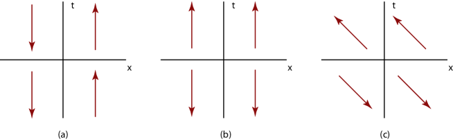
Figure 3: Three possible time-arrows, shown in the covering space $\mathbb{R}^{1,1}$. The time orientation line bundle is not orientable in the quotient; consequently, a time function possesses zeroes along some locus; there are three distinct choices.

This leads to the other main difference with Euclidean orbifold theories. Since the $\mathbb{Z}_{2}$ identification also involves time reflection, forward and backward propagating quanta are identified. Thus, when we consider string theory or quantum field theory on the orbifold, we must start with a doubled free particle Fock space involving sectors with both sign choices of energy,

$${\cal H}^{+} = \prod_{\vec{k}}{\cal H}^{+}_{\vec{k}}\ \ \ \ {\rm with}\ k^{0}=\omega_{\vec{k}}>0$$

$${\cal H}^{-} = \prod_{\vec{k}}{\cal H}^{-}_{\vec{k}}\ \ \ \ {\rm with}\ k^{0}=-\omega_{\vec{k}}<0$$ (2)

so the full Fock space is the direct sum

$${\cal H}={\cal H}^{+}\oplus{\cal H}^{-}\ .$$ (3)

The $\mathbb{Z}_{2}$ action then acts as an isomorphism $\cal{H}^{\pm}\rightarrow\cal{H}^{\mp}$ and the invariant Fock space is

$${\cal H}_{inv}={\cal H}/\mathbb{Z}_{2}\ .$$ (4)

For example, 1-particle states have the form

$$|\omega_{\vec{k}},\vec{k}\rangle_{inv}=\frac{1}{\sqrt{2}}\left(\begin{array}[]{c}|+\omega_{\vec{k}},+\vec{k}\rangle\\ |-\omega_{\vec{k}},-\vec{k}\rangle\end{array}\right)\ .$$ (5)

In this paper we will specifically consider on-shell states in closed string theory. Since the lower half of the covering space is the mirror image of the upper half, it is convenient to introduce a notation $X^{\prime}=(X^{\prime 0},X^{\prime i})=(-X^{0},-X^{i})$ for the vertex operators while using standard notation for the momentum $k$, such that $k^{0}>0$ for non-tachyonic states. Thus, for example, in bosonic string theory the lowest invariant states are

$$|V_{T}\rangle_{inv}=\frac{1}{\sqrt{2}}\left(\begin{array}[]{c}e^{ik\cdot X}|0\rangle\\ e^{ik\cdot X^{\prime}}|0\rangle\end{array}\right)\ ;\ |V^{\mu\nu}\rangle_{inv}=\frac{1}{\sqrt{2}}\left(\begin{array}[]{c}\partial X^{\mu}\bar{\partial}X^{\nu}e^{ik\cdot X}|0\rangle\\ \partial X^{\prime\mu}\bar{\partial}X^{\prime\nu}e^{ik\cdot X^{\prime}}|0\rangle\end{array}\right)\ ,$$ (6)

with the on-shell condition $M^{2}=-k^{2}=-8/l^{2}_{s},\ 0$, respectively. We will return to this formalism later in the paper, in Section 6.

3 Fractional branes in Euclidean orbifolds

The novel feature of Euclidean orbifold theories is the existence of fractional branes, localized at the orbifold fixed points. In this section we review the role of Chan-Paton indices in the construction of branes in the non-compact Euclidean $\mathbb{R}^{D}/\mathbb{Z}_{2}$ orbifold models (with a single fixed point). The route we will take is to deduce the fractional brane boundary states from the open string partition function with Chan-Paton indices. This formalism will be carried over later to the case of deformed boundary states, and to Lorentzian signature.

Begin with a D-brane which is pointlike in the directions of the orbifold. An open string in the covering space then sees two D-branes, at $X$ and $-X$. Consequently there are 4 types of open strings which are labeled by the branes upon which they end, summarized by the Chan-Paton matrix

$$\lambda=\left(\begin{array}[]{cc}D0-D0&D0-D0^{\prime}\\ D0^{\prime}-D0&D0^{\prime}-D0^{\prime}\\ \end{array}\right).$$ (7)

The $\mathbb{Z}_{2}$ action exchanges the brane and image brane, in the above basis the group elements are represented by

$$\gamma(e)=\left(\begin{array}[]{cc}1&0\\ 0&1\\ \end{array}\right)\ ,\ \gamma(g)=\left(\begin{array}[]{cc}0&1\\ 1&0\\ \end{array}\right).$$ (12)

At the fixed point, the representation is reducible, and it is useful to work in a different basis where

$$\gamma(e)=\left(\begin{array}[]{cc}1&0\\ 0&1\\ \end{array}\right)\ ,\ \gamma(g)=\left(\begin{array}[]{cc}1&0\\ 0&-1\\ \end{array}\right).$$ (17)

Fractional branes are associated with the irreducible one-dimensional representations. In the closed string language, they are described by boundary states which we denote by $|D,\alpha\rangle_{frac}$, with $\alpha=\pm$.

Now consider the open string partition function, corresponding to an annulus diagram. Take the open string to be suspended between two fractional branes at the same fixed point, with labels $\alpha,\beta$. This is encoded in the partition function by inserting appropriate projection operators $P_{\alpha},P_{\beta}$ for each boundary into the Chan-Paton traces. They impose the projection into the two irreducible representations, and are given by

$$P_{+}=\left(\begin{array}[]{cc}1&0\\ 0&0\\ \end{array}\right)\ ,\ P_{-}=\left(\begin{array}[]{cc}0&0\\ 0&1\\ \end{array}\right).$$ (22)

The projection operators are then inserted into the open string partition function as follows:

$$Z_{DD}^{\alpha,\beta} = \frac{1}{2}\left([\hbox{tr}~{}P_{\alpha}\gamma(e)][\hbox{tr}~{}P_{\beta}\gamma(e)^{-1}]~{}{\rm Tr}\ e^{-\beta H}+[\hbox{tr}~{}P_{\alpha}\gamma(g)][\hbox{tr}~{}P_{\beta}\gamma(g)^{-1}]~{}{\rm Tr}\ ge^{-\beta H}\right)$$ (23)

$$= \frac{1}{2}\left({\rm Tr}\ e^{-\beta H}+\epsilon_{\alpha\beta}{\rm Tr}\ ge^{-\beta H}\right)\ ,$$

with $\epsilon_{\pm,\pm}=1$ and $\epsilon_{\pm,\mp}=-1$. Cardy’s condition then relates the one-loop open string partition function to the tree level closed string exchange between fractional brane boundary states,

$$Z_{DD}^{\alpha,\beta}\to\mbox{}_{frac}\langle D,\alpha|\Delta(\tilde{q})|D,\beta\rangle_{frac}\ .$$ (24)

It is natural to isolate the untwisted $|\cdot\rangle_{U}$ and twisted $|\cdot\rangle_{T}$ sector boundary states, normalized as

$$\mbox{}_{U}\langle D|\Delta|D\rangle_{U}=Tr\ e^{-\beta H},\ \ \ \ \mbox{}_{T}\langle D|\Delta|D\rangle_{T}=Tr\ ge^{-\beta H}\ .$$ (25)

From (23), we then read off the fractional boundary states as linear combinations

$$|D,\alpha\rangle_{frac}=A_{\alpha}|D\rangle_{U}+B_{\alpha}|D\rangle_{T}$$ (26)

with the coefficients

$$A_{\pm}=\frac{1}{\sqrt{2}},\ \ \ \ B_{\pm}=\pm\frac{1}{\sqrt{2}}\ .$$ (27)

In other words, the two fractional states are

$$|D,\pm\rangle=\frac{1}{\sqrt{2}}\left(|D\rangle_{U}\pm|D\rangle_{T}\right)\ .$$ (28)

The regular representation is the direct sum of irreducible representations, associated to $P_{+}+P_{-}$. Thus, the regular D-brane is identified with $|D_{o}\rangle=|D,+\rangle_{frac}+|D,-\rangle_{frac}=\sqrt{2}|D\rangle_{U}$. One can check that this correctly accounts for the factors of two and such that occur in the analysis away from the fixed points.

The calculations in the following sections will actually involve deformations away from Neumann-Neumann amplitude. However, because varying the strength of the deformation parameter smoothly interpolates between Neumann and Dirichlet boundary conditions, the Chan-Paton structures can be treated in essentially the same manner as discussed above.

4 Summary of CFT Results

We now carefully summarize the results of the companion paper [21]. Depending on the choice of radius, there are different computational techniques available and different results.

4.1 The Free Theory

First we recall that in free open string theory on a circle of radius $R$, the Neumann-Neumann annulus amplitude has the form [22]

$${\cal A}_{NN}(\Delta\theta)=\frac{1}{\eta(q)}\sum_{n}q^{\alpha^{\prime}(n/R+\Delta\theta/2\pi R)^{2}}\ .$$ (29)

where we have allowed for a Wilson line $\Delta\theta$. Here, $q=e^{-\pi t}$ and this has been written in the open string channel. By Poisson resummation this becomes, with $\tilde{q}=e^{-2\pi/t}$,

$${\cal A}_{NN}=\frac{R}{\sqrt{2\alpha^{\prime}}\eta(\tilde{q}^{2})}\sum_{m\in\mathbb{Z}}(\tilde{q}^{2})^{m^{2}R^{2}/4\alpha^{\prime}}e^{-im\Delta\theta}\ .$$ (30)

This result may be factorized on the lowest lying closed string states [23]

$${\cal A}_{NN}(\Delta\theta)\equiv\langle N,\theta|\Delta(\tilde{q})|N,\theta+\Delta\theta\rangle$$ (31)

where $\Delta(\tilde{q})$ is the closed string propagator. We may then deduce the Neumann boundary state in oscillator form,

$$|N,\theta\rangle=2^{-1/4}e^{\sum_{k}\alpha_{k}\tilde{\alpha}_{k}}|0\rangle_{Fock}\otimes\sum_{m\in\mathbb{Z}}e^{im\theta}|\frac{mR}{\alpha^{\prime}},-\frac{mR}{\alpha^{\prime}}\rangle\ .$$ (32)

It has zero momentum, and is at fixed $\tilde{X}\equiv X_{L}-X_{R}$. Applying T-duality, we may obtain the Dirichlet boundary state at dual radius $\tilde{R}=\alpha^{\prime}/R$,

$$|D,x\rangle=2^{-1/4}e^{-\sum_{k}\alpha_{k}\tilde{\alpha}_{k}}|0\rangle_{Fock}\otimes\sum_{n\in\mathbb{Z}}e^{-inx_{0}/\tilde{R}}|\frac{n}{\tilde{R}},\frac{n}{\tilde{R}}\rangle$$ (33)

for a D-brane located at point $x_{0}$ in the dual circle.

At infinite radius, the Wilson line of the Neumann state is effectively projected to zero, while in the Dirichlet state, the momentum becomes continuous.

At self-dual radius, $R=\sqrt{\alpha^{\prime}}$, the conformal dimensions are square integers, and the spectrum can be classified by an $\widehat{SU(2)}$ current algebra (see e.g. [24]). To make it explicit, (30) can be rewritten in the form [25]

$${\cal A}_{NN}=\frac{1}{\sqrt{2}}\sum_{j=0,1/2,1,\ldots}\chi_{j^{2}}^{Vir}(\tilde{q}^{2})\chi_{j}^{SU(2)}(e^{-2i\Delta\theta J_{0}^{3}})$$ (34)

with $SU(2)$ characters

$$\chi_{j}^{SU(2)}(g)=Tr_{j}{\cal D}^{(j)}(g)\ ,$$ (35)

where ${\cal D}^{(j)}(g)$ is the matrix representing the $SU(2)$ element $g$ in representation $j$, and Virasoro characters

$$\chi_{j^{2}}^{Vir}(\tilde{q}^{2})=\frac{\tilde{q}^{2j^{2}}-\tilde{q}^{2(j+1)^{2}}}{\eta(\tilde{q}^{2})}\ .$$ (36)

Finally, one often uses Ishibashi states, with the normalization

$$\langle\langle j,m,n|\Delta(\tilde{q})|j^{\prime},m^{\prime},n^{\prime}\rangle\rangle=\chi_{j^{2}}^{Vir}(\tilde{q}^{2})\delta_{jj^{\prime}}\delta_{mm^{\prime}}\delta_{nn^{\prime}}$$ (37)

to express the boundary state explicitly in the $\widehat{SU(2)}$ basis

$$|N,\theta\rangle=2^{-1/4}\sum_{j=0,1/2,1,\ldots}\sum_{m,n=-j}^{j}{\cal D}^{(j)}_{m,n}(e^{-2i\theta J_{0}^{3}})|j,-m,n\rangle\rangle\ .$$ (38)

4.2 The Free Orbifold Theory

The $\mathbb{Z}_{2}$ orbifold is implemented in the open string sector, apart from Chan-Paton factors, by a projection operator $\frac{1}{2}(1+g)$. The first ’1’ term is proportional to the results of the last subsection, and gives rise to untwisted boundary states. The $g$ term will give rise to twisted boundary states. Note that at finite radius, there are two fixed orbifold points at $x=0$ and $x=\pi R$; correspondingly, there are two discrete Wilson lines at $\theta=0,\pi$ that are fixed by the orbifold.

At self-dual radius, we find

$$Z_{g;NN} \equiv Tr\ gq^{L_{0}-1/24}$$ (39)

$$= \frac{1}{\eta(q)}\sum_{n\in\mathbb{Z}}(-1)^{n}q^{n^{2}}$$ (40)

$$= \frac{1}{\sqrt{2}}\frac{1}{\eta(\tilde{q}^{2})}\sum_{m\in\mathbb{Z}}(\tilde{q}^{2})^{(m-1/2)^{2}/4}\ .$$ (41)

Writing a boundary state for the twisted states only is complicated by the presence of two fixed points. In a later section, we will show how the lowest lying twisted modes contribute to the boundary states.

It is interesting to note that, at the self-dual radius, the orbifold partition function is T-dual to an unorbifolded partition function at twice the self-dual radius [26]. In making this equivalence we exchange the $J^{3}$ current at twice the self-dual radius with the $J^{1}$ current of the self-dual radius theory. Consider again the orbifold partition function

$$Z_{NN}=\frac{1}{2}~{}Tr\ (1+g)q^{L_{0}-1/24}=\frac{1}{\eta(q)}\sum_{n\in\mathbb{Z}}q^{n^{2}}\left(\frac{1+(-1)^{n}}{2}\right)\ .$$ (42)

Clearly, $n$ must be even, and we can re-write this as

$$Z_{NN}=\frac{1}{\eta(q)}\sum_{n\in\mathbb{Z}}q^{4n^{2}}$$ (43)

which indeed is the partition function at radius $R=\sqrt{\alpha^{\prime}}/2$. After rewriting it in the closed string channel, and T-dualizing to radius $\tilde{R}=2\sqrt{\alpha^{\prime}}$, we find the Dirichlet boundary state with zero modes

$$|D,x\rangle\sim\sum_{m\in\mathbb{Z}}e^{-imx_{0}/2\sqrt{\alpha^{\prime}}}|\frac{m}{2\alpha^{\prime}},\frac{m}{2\alpha^{\prime}}\rangle\ .$$ (44)

For different discrete values of $x_{0}$, we have boundary states which correspond to fractional brane states in the orbifold theory. This implies a relationship between fractional branes in the self-dual radius theory, and D-branes at twice the self-dual radius [27]. We will elaborate this in section 4.3.1. If we allow for the possibility of branes centered at differing positions in the twice self-dual theory, we find

$$Z^{DD}_{R=2R_{s.d.}}=\frac{1}{\eta(q)}\sum_{n\in\mathbb{Z}}q^{(2n+\Delta x_{0}/2\pi\sqrt{\alpha^{\prime}})^{2}}\ .$$ (45)

4.3 The Deformed Theory

Now we consider the boundary perturbation

$$S_{\lambda}=\int_{\partial\Sigma}ds\ \left[\lambda_{+}e^{X^{0}(s)/\sqrt{\alpha^{\prime}}}+\lambda_{-}e^{-X^{0}(s)/\sqrt{\alpha^{\prime}}}\right]$$ (46)

Classically (using the correlators of the undeformed theory), this perturbation is marginal, that is $h_{cl}=1$. For $\lambda_{\pm}=(\lambda/2)e^{\pm X^{0}_{0}/\sqrt{\alpha^{\prime}}}$, this is related to the “full S-brane” [12], while for $\lambda_{-}=0$, we have the “half S-brane” [28]. The full S-brane corresponds to a process where a carefully fine-tuned initial closed string configuration time evolves to form an unstable D-brane which then decays to a final state of closed strings only. The whole process is centered around the time $X^{0}_{0}$ and is time reflection invariant about it, as evident from writing the deformation in the form

$$S_{\lambda}=\lambda\int_{\partial\Sigma}ds~{}\cosh[(X^{0}(s)-X^{0}_{0})/\sqrt{\alpha^{\prime}}]\ ,$$ (47)

in particular the initial state of closed strings is a time reflection image of the final state. The deformation was known to be exactly marginal by Wick rotation. Wick rotating $X^{0}=iX$, it becomes

$$S_{\lambda}=-\lambda\int_{\partial\Sigma}ds~{}\cos[(X(s)-X_{0})/\sqrt{\alpha^{\prime}}]\ ,$$ (48)

which is a known exactly marginal deformation. In practise, computations in the background (47) are first performed in the Euclidean signature with (48), and the results are then Wick rotated back to the Lorentzian signature.

One could absorb the parameter $X_{0}$ into the definition of the origin of time. However, for a worldsheet with multiple boundaries, there can be a distinct deformation for each boundary component. For example, if we consider the annulus, we will consider a boundary deformation of the form

$$S_{int}=-\lambda\int_{\partial\Sigma_{1}}ds\cos\left(\frac{X-X^{(1)}_{0}}{\sqrt{\alpha^{\prime}}}\right)-\tilde{\lambda}\int_{\partial\Sigma_{2}}ds\cos\left(\frac{X-X^{(2)}_{0}}{\sqrt{\alpha^{\prime}}}\right)$$ (49)

where $\partial\Sigma_{j}$ are the boundary components. This is essentially a Chan-Paton structure. Indeed in the presence of multiple branes, $\lambda$ and $\tilde{\lambda}$ would be replaced by matrices, and the annulus would include overall traces for each boundary component. For simplicity, we will assume that the $\lambda$ deformations are diagonal. A priori, there is no need to take the cosines to be centred at the same point on different boundaries, and the difference cannot be absorbed to the choice of the time origin.

4.3.1 The Orbifold Case

In the orbifold $\mathbb{R}^{1,d}/\mathbb{Z}_{2}$ the $\mathbb{Z}_{2}$ acts by $(X^{0},X^{1},\ldots,X^{d})\rightarrow-(X^{0},X^{1},\ldots,X^{d})$. After Wick rotation $X^{0}=iX$, we obtain an Euclidean orbifold $\mathbb{R}^{d+1}/\mathbb{Z}_{2}$, where $\mathbb{Z}_{2}$ acts by $(X,X^{1},\ldots,X^{d})\rightarrow-(X,X^{1},\ldots,X^{d})$. The full S-brane deformation is invariant under the orbifold identifications, if we choose it to be centered around $X^{0}=0$. In the Euclidean signature, for worldsheets with multiple boundaries, if allow for distinct deformations at each boundary component $\partial\Sigma_{j}$, we would then need each of them to be centered around $X=0$ (i.e., set $X^{(j)}_{0}=0$, but the associated parameters $\lambda_{j}$ can be independent of one another). Wick rotation back to Lorentzian signature is subtle, because of the issues with the branching of time’s arrow. This will be discussed in Section 6.

The Infinite Radius

Our basic task, performed in [21], is to compute the annulus partition function for the deformed orbifold theory. The techniques available to us depend on the choice of radius. In the non-compact case, the deformation (without the orbifold) was studied in [29] (see also [30]). The orbifold insertion was considered in [21]. An infinite radius requires the use of fermionization techniques. The boundary deformation is then written as a sum of fermionic bi-linears. The resulting action is quadratic in the fermion fields. The non-compact partition functions are:

$$Z_{1}=\frac{1}{\eta(q)}\int_{0}^{1}d\zeta_{-}\sum_{m\in\mathbb{Z}}q^{(m+\alpha(\zeta_{-}))^{2}}$$ (50)

and

$$Z_{g}=\frac{1}{\eta(q)}\sum_{\zeta_{-}=0,1/2}\sum_{m\in\mathbb{Z}}(-1)^{m}q^{(m+\alpha(\zeta_{-}))^{2}}\ .$$ (51)

Here,

$$\sin\pi\alpha=\left(\sin^{2}\left(\frac{\pi}{2}(\lambda-\tilde{\lambda})\right)\cos^{2}\left(\pi\zeta_{-}\right)+\cos^{2}\left(\frac{\pi}{2}(\lambda+\tilde{\lambda})\right)\sin^{2}\left(\pi\zeta_{-}\right)\right)^{1/2}.$$ (52)

In both expressions, $\zeta_{-}$ corresponds to the fractional part of the open string’s momenta.

The Finite Radius

If one is interested in the deformed orbifold theory at finite radius one can construct that theory, in the particular case of a rational radius, by implementing a suitable projection (a translation orbifold). At self-dual radius one may also use the adsorption technique because the boundary deformation is proportional to an $\widehat{su(2)}$ generator. The function $Z_{1}$ was computed at self-dual radius in [31]. In [21], this result was reviewed and clarified and the function $Z_{g}$ was computed. The self-dual results are:

$$Z_{1;\lambda,\tilde{\lambda}}=\frac{1}{\eta(q)}\sum_{n\in\mathbb{Z}}q^{(n+(\lambda-\tilde{\lambda})/2)^{2}}$$ (53)

$$Z_{g;\lambda,\tilde{\lambda}}=\frac{1}{\eta(q)}\sum_{n\in\mathbb{Z}}(-)^{n}q^{(n+(\lambda-\tilde{\lambda})/2)^{2}}\ .$$ (54)

Note that if we add these results we get a partition function of a theory on a circle of twice the self-dual radius,

$$Z_{\lambda,\tilde{\lambda}}=\frac{1}{\eta(q)}\sum_{n\in\mathbb{Z}}q^{(2n+\Delta\lambda/2)^{2}}\ ,$$ (55)

with $\Delta\lambda=\lambda-\tilde{\lambda}$. This can be identified with the previous partition function (45) for D-branes in the twice self-dual radius circle theory, with the identification

$$\Delta x_{0}=\Delta\lambda\pi\sqrt{\alpha^{\prime}}\ .$$ (56)

The parameter $x_{0}$ plays the role of the center-of-mass coordinate of the D-brane in the $2R_{s.d.}$ theory, whereas the parameter $\lambda$ is associated with varying the open string boundary conditions in the $R_{s.d.}$ orbifold theory. The relationship between deforming through the fractional branes in the $R_{s.d.}$ orbifold theory and the D-branes in the $2R_{s.d.}$ theory is shown in Fig. 4, elaborating upon [27].

Figure 4: Comparison between the boundary states in orbifold at self-dual radius and circle theory at twice self-dual radius. On the right diagram, $0$ and $r_{0}$ refer to fixed point values, while $\pm$ refer to the $Z_{2}$ representation each fractional brane realizes.

5 The Boundary State Interpretation

Having described open string partition functions, the next task is to pull out interesting space-time physics in the closed string channel. We consider the calculation of the overlap between the deformed boundary state and various closed string states; these correspond to one-point functions on the disk. Here we will be interested in extracting the overlap with lowest lying closed string states, as they contain information about the center of mass position. In the untwisted sector, this is the tachyon, and this problem has been studied extensively ([32] is a review). The overlap with the tachyonic vacuum in the infinite radius theory is the function

$$f_{\lambda}(x)=\frac{1}{1+e^{ix}\sin(\pi\lambda)}+\frac{1}{1+e^{-ix}\sin(\pi\lambda)}-1\ ,$$ (57)

also corresponding to the open string disk partition function in the S-brane background.

One could attempt to get at these results by factorization of the annulus amplitudes in the closed string channel. The idea would be that we can try to isolate the disk amplitudes via

$$\langle B;\tilde{\lambda}|\Delta|B;\lambda\rangle\to\sum_{\psi}\langle\psi|B;\tilde{\lambda}\rangle^{*}\Delta_{\psi}\langle\psi|B;\lambda\rangle$$ (58)

and we want to isolate $\langle\psi|B;\lambda\rangle$ for suitable $\psi$. In the untwisted sector, we would like $|\psi\rangle$ to be a momentum $p$ tachyon. We have

$$Z_{1} = \frac{1}{\sqrt{2}}\frac{1}{\eta(\tilde{q}^{2})}\int_{0}^{1}d\zeta_{-}\sum_{n\in\mathbb{Z}}(\tilde{q}^{2})^{n^{2}/4}e^{2\pi i\alpha(\zeta_{-})n}$$ (59)

Because we are interested in information describing the center of mass positions, we need to isolate the contributions of Virasoro primaries that do not correspond to oscillator excitations. This subset of states will build up $f_{\lambda}(x)$.

5.1 Untwisted Sector: Self-Dual Radius

At self-dual radius, we have $\zeta_{-}=0$, and $\alpha=(\lambda-\tilde{\lambda})/2$, so the amplitude becomes

$$Z_{1;sd} = \frac{1}{\sqrt{2}}\frac{1}{\eta(\tilde{q}^{2})}\sum_{n\in\mathbb{Z}}(\tilde{q}^{2})^{n^{2}/4}e^{i\pi(\lambda-\tilde{\lambda})n}$$ (60)

It is tempting to simply take the above amplitude and discard the eta function $\eta(\tilde{q}^{2})$, as this is usually associated with oscillator contributions. We would obtain a phase $e^{i\pi\lambda n}$ for each $n$. However, this would not give the proper $f_{\lambda}(x)$. The issue here is that the discrete primaries are also built out of the oscillators. We should subtract the contributions from both conformal descendants and the discrete primaries to identify the quantity $f_{\lambda}(x).$ This is in fact what the $SU(2)$ formalism does for us – it converts the annulus to the true Virasoro character, and gives a coefficient which is related to an $SU(2)$ character,

$$Z_{1} = \frac{1}{\sqrt{2}}\sum_{j=0,1/2,1,\ldots}\chi^{Vir}_{j^{2}}(\tilde{q}^{2})\sum_{m=-j}^{j}\mathcal{D}^{(j)}_{m,m}\left(e^{2\pi i(\lambda-\tilde{\lambda})J^{1}}\right)\ .$$

This factorizes into the Ishibashi states ${\cal D}_{-m,n}(e^{2\pi i\lambda J^{1}})|j,m,n\rangle\rangle$. The non-oscillator parts of this correspond to $m,n=\pm j$ and we arrive at

$$\sum_{p}e^{ipx}\langle p,p|B;\lambda\rangle_{sd} = {\cal D}_{-j,j}(\cdot)\sum_{p}e^{ipx}\langle p,p|j,j,j\rangle\rangle+{\cal D}_{j,-j}(\cdot)\sum_{p}e^{ipx}\langle p,p|j,-j,-j\rangle\rangle$$

$$+{\cal D}_{-j,-j}(\cdot)\sum_{p}e^{ipx}\langle p,p|j,j,-j\rangle\rangle+{\cal D}_{j,j}(\cdot)\sum_{p}e^{ipx}\langle p,p|j,-j,j\rangle\rangle$$

$$= \sum_{m}e^{imx}(-\sin\pi\lambda)^{|m|}+\sum_{m}e^{im\tilde{x}}(i\cos\pi\lambda)^{|m|}\equiv f_{\lambda}(x)+\tilde{f}_{\lambda}(\tilde{x})\ ,$$ (62)

where we reintroduced the variable $\tilde{x}$, T-dual of $x$. It is also possible to study the overlaps of boundary states with low lying states within the dual theory on the circle of twice the self-dual radius. In this case however, there are some subtleties involving the identification of zero modes in the two representations.

5.2 Untwisted Sector: Infinite Radius

At infinite radius, this computation simplifies: the $\bar{f}$ contribution decouples. We can see this directly given our infinite radius expression

$$Z_{1}=\frac{1}{\sqrt{2}}\frac{1}{\eta(\tilde{q}^{2})}\int_{0}^{1}d\zeta_{-}\sum_{m\in\mathbb{Z}}(\tilde{q}^{2})^{m^{2}/4}e^{2\pi i\alpha(\zeta_{-})m},$$ (63)

in the closed channel. Fortunately, once this is rewritten in terms of the Virasoro character, analogous to the above discussion, the $\zeta_{-}$ integral is easily performed. The net effect is to reduce the result to

$$\sum_{p}e^{ipx}\langle p,p|B;\lambda\rangle_{\infty} = {\cal D}_{-j,j}(\cdot)\sum_{p}e^{ipx}\langle p,p|j,j,j\rangle\rangle+{\cal D}_{j,-j}(\cdot)\sum_{p}e^{ipx}\langle p,p|j,-j,-j\rangle\rangle$$

$$= \sum_{m}e^{imx}(-\sin\pi\lambda)^{|m|}$$

$$= \frac{1}{1+e^{ix}\sin(\pi\lambda)}+\frac{1}{1+e^{-ix}\sin(\pi\lambda)}-1=f_{\lambda}(x)\ ,$$ (65)

so we have rederived (57).

5.3 Twisted Factorization: Self-Dual Radius

Now in the twisted sector, we can follow the same path. Here, it is in fact easier, because there is no subtlety concerning the Virasoro character – it is just what appears in the amplitude

$$Z_{g}=\frac{1}{\sqrt{2}}\frac{1}{\eta(\tilde{q}^{2})}\sum_{\zeta_{-}}\sum_{m\in\mathbb{Z}}(\tilde{q}^{2})^{(m-1/2)^{2}/4}e^{2\pi i\alpha(\zeta_{-})(m-1/2)}\ .$$ (66)

The non-oscillator part of this corresponds to the $m=0,1$ contributions. Recall that there are no zero modes in the twisted sectors, so we just need to carefully enumerate the states that are contributing to the partition function. We note that since we have considered the most general deformation (with separate deformations $\lambda$,$\tilde{\lambda}$ on each boundary), we have enough information to do so.

At self-dual radius, we have only $\zeta_{-}=0$, and the amplitude reduces to

$$Z_{g}=\frac{1}{\sqrt{2}}\frac{1}{\eta(\tilde{q}^{2})}\sum_{m\in\mathbb{Z}}(\tilde{q}^{2})^{(m-1/2)^{2}/4}e^{i\pi(\lambda-\tilde{\lambda})(m-1/2)}\ .$$ (67)

Keeping only $m=0,1$, we find

$$Z_{g,vac}=\frac{1}{\sqrt{2}}(\tilde{q}^{2})^{1/16}\left[e^{i\pi(\lambda-\tilde{\lambda})/2}+e^{-i\pi(\lambda-\tilde{\lambda})/2}\right]\ .$$ (68)

The ability to separate this amplitude into two factors depending on either $\lambda$ or $\tilde{\lambda}$ only, implies that there are two orthogonal states contributing here, which we will denote by $|I\rangle_{T}$ and $|II\rangle_{T}$. We are finding that

$$|B,\lambda;0\rangle_{T;sd}=2^{-1/4}e^{i\pi\lambda/2}|I\rangle_{T}+2^{-1/4}e^{-i\pi\lambda/2}|II\rangle_{T}\ .$$ (69)

We re-emphasize here that we are not considering the full boundary state, but really only its overlap with the twisted vacua. The full boundary state contains oscillator excitations as well. However, the dependence on the twisted vacua already contains the information about the space-time positions.

At $\lambda=0$, this reduces to

$$|B,0;0\rangle_{T;sd}=2^{-1/4}(|I\rangle_{T}+|II\rangle_{T})\equiv|N,0;0\rangle_{T;sd}\ ,$$ (70)

which must coincide with one of the usual Neumann states [22]. We will verify this below. Further, at $\lambda=1$, it reduces to

$$|B,1;0\rangle_{T;sd}=i2^{-1/4}(|I\rangle_{T}-|II\rangle_{T})\equiv|N,1;0\rangle_{T;sd}\ ,$$ (71)

which must be the other Neumann state. Note that these two states are orthogonal. Next consider the Dirichlet states. We should get these by deforming to $\lambda=1/2$ and $\lambda=-1/2$. The former corresponds to a D0-brane at the fixed point $X=0$, the latter to a D0-brane at $X=\pi\sqrt{\alpha^{\prime}}$. So we identify

$$|B,1/2;0\rangle_{T;sd}=2^{-1/4}(e^{+i\pi/4}|I\rangle_{T}+e^{-i\pi/4}|II\rangle_{T})\equiv|0\rangle_{T}$$ (72)

and

$$|B,-1/2;0\rangle_{T;sd}=2^{-1/4}(e^{-i\pi/4}|I\rangle_{T}+e^{+i\pi/4}|II\rangle_{T})\equiv|\pi\sqrt{\alpha^{\prime}}\rangle_{T}\ .$$ (73)

These states were called $|D(\phi_{0})_{T}\rangle$ with $\phi_{0}=0,\pi r$ respectively in [22] ($r=\sqrt{\alpha^{\prime}}$ for selfdual radius). Note that they are orthogonal. Now we can represent the states that we called $|I\rangle_{T},|II\rangle_{T}$ in terms of the Dirichlet states:

$$|I\rangle_{T} = 2^{-3/4}(e^{-i\pi/4}|0\rangle_{T}+e^{i\pi/4}|\pi\sqrt{\alpha^{\prime}}\rangle_{T})$$

$$|II\rangle_{T} = 2^{-3/4}(e^{i\pi/4}|0\rangle_{T}+e^{-i\pi/4}|\pi\sqrt{\alpha^{\prime}}\rangle_{T})$$

and plug these back into the general expression for the deformed twisted boundary state (69). We obtain

$$|B,\lambda;0\rangle_{T}=\cos\left[\frac{\pi}{2}(\lambda-\frac{1}{2})\right]|0\rangle_{T}+\cos\left[\frac{\pi}{2}(\lambda+\frac{1}{2})\right]|\pi\sqrt{\alpha^{\prime}}\rangle_{T}\ .$$ (74)

At $\lambda=0,1$ we then obtain the two Neumann boundary states

$$|N,0;0\rangle = 2^{-1/2}(|0\rangle_{T}+|\pi\sqrt{\alpha^{\prime}}\rangle_{T})$$

$$|N,1;0\rangle = 2^{-1/2}(|0\rangle_{T}-|\pi\sqrt{\alpha^{\prime}}\rangle_{T})\ .$$ (75)

These agree with the expressions in [22]. In fact, [22] assumed the form of the two twisted Neumann boundary states. Here we have derived them by deforming from known (Dirichlet) states.

5.4 Twisted Factorization: Infinite Radius

It is instructive to also look at this factorization in the infinite radius theory. In this case, both $\zeta_{-}=0$ and $\zeta_{-}=1/2$ contribute and we arrive at

$$Z_{g}=\frac{1}{\sqrt{2}}\frac{1}{\eta(\tilde{q}^{2})}\sum_{m\in\mathbb{Z}}(\tilde{q}^{2})^{(m-1/2)^{2}/4}\left[e^{i\pi(\lambda-\tilde{\lambda})(m-1/2)}+e^{i\pi(\lambda+\tilde{\lambda}-1)(m-1/2)}\right]\ .$$ (76)

The contribution of the twisted vacua is

$$Z_{g,vac}=\frac{1}{\sqrt{2}}(\tilde{q}^{2})^{1/16}\left[e^{i\pi(\lambda-\tilde{\lambda})/2}+e^{-i\pi(\lambda-\tilde{\lambda})/2}+e^{i\pi(\lambda+\tilde{\lambda}-1)/2}+e^{-i\pi(\lambda+\tilde{\lambda}-1)/2}\right]\ .$$ (77)

We note that this expression factorizes

$$Z_{g,vac}=\frac{1}{\sqrt{2}}(\tilde{q}^{2})^{1/16}\left[e^{-i\pi\tilde{\lambda}/2}-ie^{i\pi\tilde{\lambda}/2}\right]\left[e^{i\pi\lambda/2}+ie^{-i\pi\lambda/2}\right]$$ (78)

and thus we interpret this as only one state contributing,

$$|B,\lambda\rangle_{T;\infty}=2^{-1/4}\left[e^{i\pi\lambda/2}+ie^{-i\pi\lambda/2}\right]|0\rangle_{T}\ .$$ (79)

Note that the state $|B,-1/2\rangle_{T;\infty}$ is orthogonal to $|B,1/2\rangle_{T;\infty}$ as well as itself: that is, it decouples. This corresponds to the fact that the second fixed point, present at finite radius, has moved off to infinity, and the corresponding twisted boundary states decouple. Similarly, by looking at integer $\lambda$, it is possible to see that $|\pi\sqrt{\alpha^{\prime}}\rangle_{T}$ decouples. Thus, at infinite radius we only obtain the contribution from the twisted sector at the remaining fixed point $X=0$.

6 Back to the Lorentzian signature

After the Euclidean computations, we will now move back to Lorentzian signature. As discussed in Section 2, in the case of the orbifold there are some subtleties. We will also be interested in analyzing how the brane decays into closed strings in the orbifold. We will compute the average total energy and number densities of the emitted untwisted closed strings and compare the calculation and the results with those of [33]. The computations involve a prescription for a time integration contour, which in turn is related to how the initial state of the brane is prepared. A natural contour to use on the orbifold turns out to be the Hartle-Hawking (HH) contour which was introduced in [33]. With this choice, on the fundamental domain we can interpret the unstable brane to nucleate at the origin of time and then decay into closed strings.

Let us first review the standard case without the orbifold. Upon Wick rotation back to the Lorentzian signature the overlap of the deformed boundary state with the vacuum becomes

$$f(x^{0})\equiv\mbox{}_{\infty}\langle 0|D(\pi\lambda)\rangle_{\infty}=\frac{1}{1+e^{x^{0}}\sin(\pi\lambda)}+\frac{1}{1+e^{-x^{0}}\sin(\pi\lambda)}-1\ .$$ (80)

The full boundary state has the structure

$$|B\rangle={\cal N}_{p}|B\rangle_{X^{0}}|B\rangle_{X}|B\rangle_{bc}$$ (81)

where

$$|B\rangle_{X^{0}}=f(x^{0})|0\rangle+\sigma(x^{0})\alpha^{0}_{-1}\tilde{\alpha}^{0}_{-1}|0\rangle+\cdots$$ (82)

with

$$\sigma(x^{0})=\cos(2\pi\lambda)+1-f(x^{0})\ .$$ (83)

To compute the overlap with any on-shell closed string state, it is convenient to express the vertex operators in the gauge

$$V=e^{iEX^{0}}V_{sp}$$ (84)

where $V_{sp}$ contains only the space part. The overlap then takes a simple form

$$\langle V|B\rangle=\langle 0|e^{iEX^{0}}|B\rangle_{X^{0}}\times{\rm(phase)}$$ (85)

yielding the amplitude

$$I(E)=i\int_{{\cal C}}dx^{0}e^{iEx^{0}}f(x^{0})$$ (86)

with a suitable choice of the integration contour ${\cal C}$.

In the case of the orbifold, the computations are simplest to perform in the covering space. As discussed in Section 2, a new feature is the need to double the Hilbert space by hand upon Wick rotating back to the Lorentzian signature. This is because on the covering space a single quantum corresponds to two copies propagating into the opposite time directions $X^{0}$ and $X^{\prime 0}=-X^{0}$. The on-shell closed string states then take the form

$$|V\rangle=\frac{1}{\sqrt{2}}\left(\begin{array}[]{c}e^{iEX^{0}}V_{sp}|0\rangle\\ e^{iEX^{\prime 0}}V^{\prime}_{sp}|0\rangle\end{array}\right)\ .$$ (89)

Similarly, the time direction part of the boundary state becomes

$$|B\rangle_{X^{0}}=\frac{1}{\sqrt{2}}\left(\begin{array}[]{c}f(x_{0})|0\rangle\\ f(x^{\prime}_{0})|0\rangle\end{array}\right)+\cdots\ .$$ (92)

Note however that

$$f(x^{\prime 0})=f(x^{0})=\frac{1}{1+e^{x^{0}}\sin(\pi\lambda)}+\frac{1}{1+e^{-x^{0}}\sin(\pi\lambda)}-1$$ (93)

because of time reflection symmetry. The overlap with the closed string state becomes

$$\langle V|B\rangle=\frac{1}{2}(e^{iEx^{0}}f(x^{0})+e^{iEx^{\prime 0}}f(x^{\prime 0}))\ .$$ (94)

Let us pause to compare the physical interpretation of the above with the standard full S-brane. The full S-brane corresponds to formation and decay of an unstable brane, centered at the origin of the time axis. On the orbifold, the full Minkowski space is replaced by the covering space, with a two-branched time direction. The unstable brane is centered at the origin of the time coordinates, but decays into closed strings propagating into the opposite time directions, as illustrated in Figure 5.

Figure 5: Untwisted closed string emission in the covering space.

For the decay amplitude calculation, we then need a contour integration prescription. The fundamental domain has a semi-infinite time axis, $X^{0}\geq 0$. We have set the decay of the brane to start at $X^{0}=0$. Since there is no past to $X^{0}=0$, we cannot build up the brane from some closed string initial state. Instead, it is most natural to adopt the prescription in [33] for “nucleating” the brane via smeared D-instantons (see also [34]) in imaginary time. This corresponds to using a Hartle-Hawking time contour, coming in from $X^{0}=i\infty$ along the imaginary time axis to the origin and then proceeding along the real time axis to $X^{0}=\infty$. For the actual calculation, we move back to the covering space where time runs from $X^{0}=0$ to opposite time directions $X^{0}\rightarrow\infty$ and $X^{\prime 0}=-X^{0}\rightarrow\infty$. The HH contour then maps to the double contour with branches (see Fig. 6.)

Figure 6: The double HH contour in the covering space.

$${\cal C}_{HH},\tilde{{\cal C}}_{HH}:\ X^{0},X^{\prime 0}=i\infty\rightarrow 0\rightarrow\infty\ .$$ (95)

Applying the contour to the overlap (94), we get

$$\langle V|B\rangle = \frac{1}{2}\int_{{\cal C}_{HH}}e^{iEx^{0}}f(x^{0})dx^{0}+\frac{1}{2}\int_{\tilde{\cal C}_{HH}}e^{iEx^{\prime 0}}f(x^{\prime 0})dx^{\prime 0}$$ (96)

$$= e^{-iE\ln\lambda}\frac{\pi}{\sinh(\pi E)}\ ,$$

as in [33] for the full brane with the HH contour. The same is true for the total average energy and average number densities for the produced untwisted closed strings on the fundamental domain. The results are the same as in the standard case,

$$\frac{\bar{N}}{V_{p}}\sim\sum_{n}n^{-1-p/4}\ ;\ \frac{\bar{E}}{V_{p}}\sim\sum_{n}n^{-1/2-p/4}\ ,$$ (97)

where the sums are over the level numbers. To conclude, in the orbifold the decay in the untwisted sector is quantitatively the same as in the usual case.

The twisted sector is more problematic conceptually. Since the twisted strings are localized in time, the concept of “producing” them in the decay is ill defined. Moreover, there are very few physical states in the twisted sector. At present we do not have much more to say about this matter.

7 Conclusions and Outlook

The decay of unstable D-branes or D-brane configurations is an important open question in string theory. They may play a crucial role in cosmology, and there already exist several scenarios making use of them. While spacetime orbifolds may be considered just toy models, capturing some features of string theory in more general time-dependent backgrounds, they are nevertheless useful for gaining insights into problems associated with quantum string theory. We have argued that the twisted sector which exists in orbifolds may contribute to the decay of unstable branes. In particular, we have presented a detailed analysis of how to implement the orbifold identifications into the decay, in a simple example, both in the open string and closed string formalism, and argued that this leads to a new class of S-branes, which we have called fractional S-branes, in analogy to the fractional branes of Euclidean orbifolds. We expect that the existence of fractional S-branes is a generic feature of spacetime orbifolds, and may reflect some physics of D-brane decay in more general time-dependent backgrounds. They may also be relevant for the question of resolution of spacelike singularities.

In particular, we have constructed a model where the D-brane decay has a semi-infinite duration, without a prior build-up phase. This is in contrast to the full S-brane and half S-brane constructions, where either the brane must first be formed from a fine-tuned closed string initial state, or the decay starts from infinite past without any parameter to control its pace. For potential applications of our construction, we can make at least the following speculative remarks.

(i) We have presented a model where an unstable brane, prepared at the “Big Bang” origin of the spacetime, stores a large amount of energy which then gets released in the decay into heavy closed string modes and the subsequent cascade into lighter excitations. Presumably the large energy backreacts into the spacetime and converts it into an expanding cosmological model. The initial condition, while defined at an initial spacelike singularity, is still under control because it has a well defined dual formulation in terms of open string worldsheet theory. If the unstable brane is taken to be volume filling, it also provides a homogeneous initial condition. This may be compared with brane cosmological models where a collision of almost parallel branes provides a homogeneous initial condition – in our case the homogeneity only involves a single brane.

(ii) The idea of an initial unstable brane at the Big Bang may be coupled with string/brane gas cosmology [35, 36]. Take the spacelike directions to be compactified to Planck Scale, and the initial unstable brane to be wrapped in all directions. The brane then decays into closed strings, which interact and presumably thermalize; thus brane decay could be viewed as the origin of the hot string gas.

(iii) In our orbifold construction, the covering space of the orbifold can be viewed as a model where two branches of spacetime originate from the same Big Bang event. One may view the other branch and the images of closed strings in it simply as a calculational trick, in analogy to the thermal ghosts in the real time formulation of finite temperature quantum field theory or thermofield dynamics. But one could also view it as a real branch of the spacetime, so that the total spacetime contains a multi-branched arrow of time.

(iv) If the other branch of the spacetime from the origin of time is viewed simply as a calculational trick, one may ask if this trick could be applied in other cases. Consider for example the setup of $D\bar{D}$-inflationary models, where a D-brane and an anti D-brane first approach each other, with the scalar excitation from interpolating open string providing the rolling inflaton, and then form an unstable system where the rolling tachyon provides an exit mechanism from inflation and may be responsible for the subsequent reheating. It is not well understood how to actually model this in the language of the open string sigma model. If the rolling tachyon has a hyperbolic cosine profile, then it contains an unwanted stage where the tachyon rolls ”up”. If it only has an exponential profile, then the decay starts at infinite past leaving no room for the inflationary stage. It may be possible to develop a model, where the decay is modeled by our construction, viewing the other branch or time direction from the origin simply as a calculational trick.

All the above comments are very tentative, but we believe they illustrate that there are exciting possibilities ahead to unravel and study.

Acknowledgments

We thank V. Balasubramanian, N. Jokela, A. Naqvi for useful discussions and comments. In particular we thank P. Kraus for discussions on boundary states and orbifolds at the early stages of this work. EKV thanks UCLAs IPAM and the organizers of the Conformal Field Theory 2nd Reunion Conference, and the organizers of the Workshop on Gravitational Aspects of String Theory at Fields Institute for hospitality while this work was in progress. SK would like to thank Matthias Gaberdiel, Andreas Recknagel, and Masaki Oshikawa for discussions, and also the organizers of the July 2005 London Mathematical Society Durham Symposium on ”Geometry, Conformal Field Theory and String Theory.” EKV was in part supported by the Academy of Finland. SK was in part supported by a JSPS fellowship. RGL and SN have support from the US Department of Energy under contract DE-FG02-91ER40709.

References

- [1] B. Durin and B. Pioline, arXiv:hep-th/0501145.
- [2] A. Hashimoto and S. Sethi, Phys. Rev. Lett. 89, 261601 (2002) [arXiv:hep-th/0208126].
- [3] M. Alishahiha and S. Parvizi, JHEP 0210, 047 (2002) [arXiv:hep-th/0208187].
- [4] L. Dolan and C. R. Nappi, Phys. Lett. B 551, 369 (2003) [arXiv:hep-th/0210030].
- [5] R. G. Cai, J. X. Lu and N. Ohta, Phys. Lett. B 551, 178 (2003) [arXiv:hep-th/0210206].
- [6] K. Okuyama, JHEP 0302, 043 (2003) [arXiv:hep-th/0211218].
- [7] Y. Hikida, R. R. Nayak and K. L. Panigrahi, JHEP 0505, 018 (2005) [arXiv:hep-th/0503148].
- [8] Y. Hikida, R. R. Nayak and K. L. Panigrahi, JHEP 0509, 023 (2005) [arXiv:hep-th/0508003].
- [9] Y. Hikida and T. S. Tai, arXiv:hep-th/0510129.
- [10] A. Sen, JHEP 0204, 048 (2002) [arXiv:hep-th/0203211].
- [11] A. Sen, JHEP 0207, 065 (2002) [arXiv:hep-th/0203265].
- [12] M. Gutperle and A. Strominger, JHEP 0204, 018 (2002) [arXiv:hep-th/0202210].
- [13] V. Balasubramanian, S. F. Hassan, E. Keski-Vakkuri and A. Naqvi, Phys. Rev. D 67, 026003 (2003) [arXiv:hep-th/0202187].
- [14] S. Kawai, E. Keski-Vakkuri, R. G. Leigh and S. Nowling, Phys. Rev. Lett. 96, 031301 (2006) [arXiv:hep-th/0507163].
- [15] E. Schrödinger, Expanding Universes. Cambride, UK: Univ. Pr. (1956).
- [16] G. W. Gibbons, Nucl. Phys. B 271, 497 (1986).
- [17] A. Folacci and N. Sanchez, Nucl. Phys. B 294, 1111 (1987).
- [18] M. K. Parikh, I. Savonije and E. P. Verlinde, Phys. Rev. D 67, 064005 (2003) [arXiv:hep-th/0209120].
- [19] M. K. Parikh and E. P. Verlinde, JHEP 0501, 054 (2005) [arXiv:hep-th/0410227].
- [20] R. Biswas, E. Keski-Vakkuri, R. G. Leigh, S. Nowling and E. Sharpe, JHEP 0401, 064 (2004) [arXiv:hep-th/0304241].
- [21] S. Kawai, E. Keski-Vakkuri, R. G. Leigh, S. Nowling, “The rolling tachyon boundary conformal field theory on an orbifold”, to appear.
- [22] M. Oshikawa and I. Affleck, Nucl. Phys. B 495, 533 (1997) [arXiv:cond-mat/9612187].
- [23] J. L. Cardy, Nucl. Phys. B 324, 581 (1989).
- [24] P. Di Francesco, P. Mathieu and D. Senechal, “Conformal field theory”, New York, USA: Springer (1997).
- [25] M. R. Gaberdiel and A. Recknagel, JHEP 0111, 016 (2001) [arXiv:hep-th/0108238].
- [26] P. H. Ginsparg, Nucl. Phys. B 295, 153 (1988).
- [27] A. Recknagel and V. Schomerus, Nucl. Phys. B 545, 233 (1999) [arXiv:hep-th/9811237].
- [28] F. Larsen, A. Naqvi and S. Terashima, JHEP 0302, 039 (2003) [arXiv:hep-th/0212248].
- [29] J. Polchinski and L. Thorlacius, Phys. Rev. D 50, 622 (1994) [arXiv:hep-th/9404008].
- [30] K. R. Kristjansson and L. Thorlacius, JHEP 0501, 047 (2005) [arXiv:hep-th/0412175].
- [31] C. G. . Callan, I. R. Klebanov, A. W. W. Ludwig and J. M. Maldacena, Nucl. Phys. B 422, 417 (1994) [arXiv:hep-th/9402113].
- [32] A. Sen, Int. J. Mod. Phys. A 20, 5513 (2005) [arXiv:hep-th/0410103].
- [33] N. Lambert, H. Liu and J. Maldacena, arXiv:hep-th/0303139.
- [34] D. Gaiotto, N. Itzhaki and L. Rastelli, Nucl. Phys. B 688, 70 (2004) [arXiv:hep-th/0304192].
- [35] R. H. Brandenberger and C. Vafa, Nucl. Phys. B 316, 391 (1989).
- [36] S. Alexander, R. H. Brandenberger and D. Easson, Phys. Rev. D 62, 103509 (2000) [arXiv:hep-th/0005212].