The index of the overlap Dirac operator on a discretized 2d non-commutative torus
Abstract:
The index, which is given in terms of the number of zero modes of the Dirac operator with definite chirality, plays a central role in various topological aspects of gauge theories. We investigate its properties in non-commutative geometry. As a simple example, we consider the U(1) gauge theory on a discretized 2d non-commutative torus, in which general classical solutions are known. For such backgrounds we calculate the index of the overlap Dirac operator satisfying the Ginsparg-Wilson relation. When the action is small, the topological charge defined by a naive discretization takes approximately integer values, and it agrees with the index as suggested by the index theorem. Under the same condition, the value of the index turns out to be a multiple of , the size of the 2d lattice. By interpolating the classical solutions, we construct explicit configurations, for which the index is of order 1, but the action becomes of order . Our results suggest that the probability of obtaining a non-zero index vanishes in the continuum limit, unlike the corresponding results in the commutative space.
KEK-TH-1059
UTHEP-515
1 Introduction
Non-commutative (NC) geometry [1, 2] has been studied for quite a long time as a simple modification of our notion of space-time at small distances possibly due to effects of quantum gravity [3]. It has attracted much attention since it was shown to appear naturally from matrix models [4, 5] and string theories [6]. In particular, field theory on NC geometry has a peculiar property known as the UV/IR mixing [7], which may cause a drastic change of the long-distance physics through quantum effects. This phenomenon has been first discovered in perturbation theory, but it was shown to appear also in a fully nonperturbative setup [8]. A typical example is the spontaneous breaking of the translational symmetry in NC scalar field theory, which was first conjectured from a self-consistent one-loop analysis [9] and confirmed later on by Monte Carlo simulation [10, 11, 12]. (See also [13, 14].)
The appearance of a new type of IR divergence due to the UV/IR mixing spoils the perturbative renormalizability in general [15], and therefore, even the existence of a sensible field theory on a NC geometry is a priori debatable. In order to study such a nonperturbative issue, one has to define a regularized field theory on NC geometry, which is possible by using matrix models. In the case of NC torus, for instance, the so-called twisted reduced model [16, 17] is interpreted as a lattice formulation of NC field theories [8], in which finite matrices are mapped one-to-one onto fields on a periodic lattice. The existence of a sensible continuum limit and hence the nonperturbative renormalizability have been shown by Monte Carlo simulations in NC U(1) gauge theory in 2d [18] and 4d [19] as well as in NC scalar field theory in 3d [12, 20].
In the case of fuzzy sphere [21], finite matrices are mapped one-to-one onto functions on the sphere with a specific cutoff on the angular momentum. The fuzzy sphere (or fuzzy manifolds [22, 23] in general) preserves the continuous symmetry of the base manifold, which makes it an interesting candidate for a novel regularization of commutative field theories alternative to the lattice [24]. It is also interesting to use fuzzy spheres in the coset space dimensional reduction [25]. Stability of fuzzy manifolds in matrix models with the Chern-Simons term [26, 27] has been studied by Monte Carlo simulations [28, 29].
One of the interesting features of NC field theories is the appearance of a new type of topological objects, which are referred to as NC solitons [30], NC monopoles, NC instantons, and fluxons [31] in the literature. They are constructed by using a projection operator, and the matrices describing such configurations are assumed to be infinite dimensional. In finite NC geometries, namely in the case where field configurations are described by finite-dimensional matrices and therefore regularized, topological objects have been constructed by using the algebraic K-theory and projective modules [32, 33, 34].
Dynamical aspects of these topological objects are important in particular in the realization of a 4d chiral gauge theory in the context of string theory compactification, which requires a nontrivial index in the compactified dimensions (See, for instance, Chapter 14 of ref. [35].) Ultimately we hope to realize such a scenario dynamically, for instance, in the IIB matrix model [36], in which the dynamical generation of four-dimensional space-time [37, 38, 39] as well as the gauge group [40, 41] has been studied intensively.
Extending the notion of the index to finite NC geometry is a nontrivial issue due to the doubling problem of the naive Dirac action. The same problem occurs also in the ordinary lattice gauge theory. There one can add the Wilson term to the Dirac action to remove the species doublers in the continuum limit at the expense of the explicit breaking of chiral symmetry. This had been a notorious problem in lattice gauge theory as manifested by the no-go theorem [42]. It was found, however, that by adopting a Dirac operator which satisfies the Ginsparg-Wilson relation [43], a modified chiral symmetry, which becomes the usual one in the continuum limit, can be exactly preserved on the lattice [44, 45]. The Dirac operator has exact zero modes with definite chirality for topologically nontrivial gauge configurations, and therefore one can define the index unambiguously [46, 47, 44]. A concrete example of such an operator with desirable properties in the continuum limit is given by the so-called overlap111Historically, the overlap formalism [46], from which one can actually derive the overlap Dirac operator [48], has been established before the rediscovery of the Ginsparg-Wilson relation. Dirac operator [48]. The index theorem for the overlap Dirac operator is studied numerically in refs. [46, 49]. The successful results obtained in these tests may be understood from the analytical work [50] (See also ref. [51] for an extension.), in which the usual expression for the topological charge in the continuum has been derived from the index of the overlap Dirac operator nonperturbatively. As emphasized in refs. [50], the derivation of the correct axial anomaly [52], which uses the perturbative expansion with respect to the gauge field, is not sufficient for demonstrating the index theorem for topologically nontrivial gauge configurations.
In the past several years, the ideas developed in lattice gauge theory have been successfully extended to NC geometry. In the case of NC torus, the overlap Dirac operator has been introduced in ref. [53], and it was used to define a NC chiral gauge theory with manifest star-gauge invariance. For general NC manifolds, a prescription to define the Ginsparg-Wilson Dirac operator and its index has been provided in ref. [54], and the fuzzy sphere was considered as a concrete example222The Ginsparg-Wilson Dirac operator for vanishing gauge field was constructed earlier in refs. [55].. The Ginsparg-Wilson algebra for the fuzzy sphere has been studied in detail in each topological sector [33]. In ref. [56] the overlap Dirac operator on the NC torus [53] was derived also from this general prescription [54], and the axial anomaly has been calculated in the continuum limit.
In an attempt to construct a topologically nontrivial configuration on the fuzzy sphere, an analogue of the ’t Hooft-Polyakov monopole was obtained [33, 34]. Although the index defined through the Ginsparg-Wilson Dirac operator vanishes for these configurations, one can make it non-zero by inserting a projection operator, which picks up the unbroken U(1) component of the SU(2) gauge group. In fact the ’t Hooft-Polyakov monopole configurations are precisely the meta-stable states observed in Monte Carlo simulations [28] taking the two coincident fuzzy spheres as the initial configuration, which eventually decays into a single fuzzy sphere. In ref. [57] this instability was studied analytically by the one-loop calculation of free energy around the ’t Hooft-Polyakov monopole configurations, and it was interpreted as the dynamical generation of a nontrivial index, which may be used for the realization of a chiral fermion in our space-time.
The primary aim of the present work is to investigate the properties of the index in finite NC geometry, taking the 2d U(1) gauge theory on a discretized NC torus as a simple example, which is studied extensively in the literature both numerically [18] and analytically [58, 59, 60]. In particular, ref. [60] presents general classical solutions carrying the topological charge. We compute the index defined through the overlap Dirac operator for these classical solutions. The topological charge defined naively on the discretized NC torus is not an integer in general, although the index is. We observe, however, that when the action is small, the topological charge is close to an integer, and it agrees with the index as suggested by the index theorem. In fact, under the same condition, the index turns out to be a multiple of , the linear size of the 2d lattice. By interpolating the classical solutions, we construct explicit configurations333While we were preparing this article, we received a preprint [61], in which a gauge configuration with non-zero index was found numerically in the same model at small . for which the index is of order 1, but the action becomes of order . Our results suggest that the probability of obtaining a non-zero index vanishes in the continuum limit, which is consistent with the instanton calculus in the continuum theory [59].
The rest of this paper is organized as follows. In section 2 we provide some generalities concerning a matrix model formulation of gauge theories on a discretized NC torus and define the index of the overlap Dirac operator. In section 3 we focus on the two-dimensional case, and discuss the classical solutions and the topological charge. In section 4 we examine whether the index theorem holds for the classical solutions. In section 5 we construct explicit configurations with the index of order 1 by interpolating the classical solutions, and study their properties. In section 6 we review some known results in the commutative case, and discuss their relationship to our results. Section 7 is devoted to a summary and discussions.
2 Generalities
2.1 gauge theory on a discretized NC torus
The U(1) gauge theory on a NC space is given by the action
| (1) | |||||
| (2) |
where the star-product is defined by
| (3) |
Note that the star-product is associative but non-commutative. This non-commutativity may be attributed to that of space-time since
| (4) |
The action (1) is invariant under a star-gauge transformation
| (5) |
where obeys the star-unitarity condition
| (6) |
instead of .
When we discretize the space, the consistency with the NC algebra inevitably requires the space to be compactified in a specific way [8]. Thus we obtain a theory on a periodic lattice with the action
| (7) |
where the link variables are star-unitary; i.e.,
| (8) |
We use the standard notation in lattice gauge theory, where represents a unit vector in the direction, and represents the lattice spacing. The star-product on the lattice can be obtained by rewriting (3) in terms of Fourier modes and restricting the momentum to be the one allowed on the lattice. As in the commutative space, one obtains the continuum action (1) from (7) in the limit with the identification and
| (9) |
2.2 the overlap Dirac operator and its index
In this section we define the overlap Dirac operator and its index for a gauge configuration on the discretized NC torus [53, 54, 56]. All the formulae have the same form as in the usual lattice gauge theory except for the use of the star product.
We consider a Dirac operator satisfying the Ginsparg-Wilson relation [43]
| (10) |
Assuming the -hermiticity , we can define a hermitian operator by
| (11) |
which may be solved for as . Then the Ginsparg-Wilson relation (10) is equivalent to requiring to be unitary. The overlap Dirac operator corresponds to taking to be [48]
| (12) | |||||
| (13) |
where is the Wilson-Dirac operator
| (14) |
with () being the covariant forward (backward) difference operator defined by
| (15) | |||||
| (16) |
Since the Ginsparg-Wilson relation (10) can be rewritten as
| (17) |
the lattice action
| (18) |
has the exact lattice chiral symmetry [44, 45]
| (19) |
Note also that the space of zero modes of the Dirac operator is invariant under , which means that one can define the index of unambiguously by , where is the number of zero modes with the chirality . It turns out that [46, 47, 44]
| (20) |
where represents a trace over the space of the Dirac spinor field on the lattice.
2.3 matrix formulation
So far we have been using a formulation of NC geometry, in which the non-commutativity of the space-time is encoded in the star-product. In fact it is much more convenient for our purpose to use an equivalent formulation [62], in which one maps functions on a NC space to operators so that the star-product becomes nothing but the usual operator product, which is non-commutative. In particular, the coordinate operators satisfy the commutation relation . In the discrete version, one maps a field on the lattice onto a matrix , where in order to match the degrees of freedom. This map yields the following correspondence
| (21) | |||||
| (22) | |||||
| (23) |
The SU() matrices () represent a shift on the matrix side, and they satisfy the ’t Hooft-Weyl algebra
| (24) |
where is a phase factor. An explicit representation of in the case shall be given in section 3.1.
Using the map, one can reformulate the lattice theory (7) in terms of matrices. The star-unitarity condition (8) on the link variables simply implies that the corresponding matrix should be unitary. The action (7) can be written as
| (25) | |||||
| (26) |
where is a U() matrix. This is nothing but the twisted Eguchi-Kawai (TEK) model [17], which appeared in history as a matrix model equivalent to the large gauge theory [16]. In fact we have added the constant term to what we would obtain from (7) in order to make the absolute minimum of the action zero. We use this convention in the rest of this paper.
The index can be calculated using eq. (20), where is defined by eq. (13). The only thing to note in transcription into matrices is that the covariant forward and backward difference operators and , which appear in the definition of the Wilson-Dirac operator (14), should now be defined as
| (27) | |||||
| (28) |
The index is simply given by half the difference between the numbers of positive and negative eigenvalues of the hermitian matrix . In this calculation we may simply set , since the lattice spacing appearing in the definition of the index actually cancels out as it should. The computational effort for calculating the index is of order , since we have to diagonalize the hermitian matrix .
3 Two-dimensional case
In this section we focus on the two-dimensional case, and discuss the classical solutions and the topological charge.
3.1 explicit representation
An explicit form of the map between fields and matrices in the two-dimensional case is given, for instance, in ref. [53], where the twist in eq. (24) is given by
| (29) |
with being an odd integer. The algebra (24) can be realized by
| (30) |
where we have defined the SU matrices
| (31) |
obeying for later convenience. For this particular construction, which we are going to use throughout this paper, it turns out that the NC tensor, which appears in the star-product, is given by
| (32) | |||||
| (33) |
Note that the linear size of the torus goes to in the continuum limit fixing . A finite torus can be obtained by other constructions given in the first paper of refs. [8] and ref. [60], which are mutually equivalent.
3.2 definition of the topological charge
Let us define the topological charge for a gauge configuration on the discretized 2d torus. In the language of fields, we define the topological charge as
| (34) |
which is obtained as a naive discretization of the topological charge in 2d gauge theory defined in the continuum as
| (35) |
By using the map between fields and matrices, the topological charge (34) can be represented in terms of matrices as
| (36) | |||||
| (37) |
3.3 classical solutions
The classical equation of motion can be obtained from the action (26) as
| (38) |
where the unitary matrix is defined by
| (39) |
The general solutions444In fact there is another type of solutions, which we do not consider in this paper since they do not have finite action in the continuum limit [60]. to this equation can be brought into a block-diagonal form [60]
| (40) |
by an appropriate SU() transformation, where are unitary matrices satisfying the ’t Hooft-Weyl algebra
| (41) | |||||
| (42) |
An explicit representation [63] is given, for instance, by
| (43) |
For each solution, the action and the topological charge can be easily evaluated as
| (44) | |||||
| (45) |
Note that the topological charge is not an integer in general. If we require the action to be less than of order , however, the argument of the sine has to vanish in the large limit for all . In that case the topological charge approaches an integer
| (46) |
which is actually a multiple of .
4 The index theorem for the classical solutions
The index theorem [64] relates the topological charge of an arbitrary gauge configuration to the index of the Dirac operator on that background. A proof of the index theorem in noncommutative is given in ref. [65]555In ref. [65] an explicit ADHM construction of the fermionic zero modes in the multi-instanton backgrounds was also performed, and the number of zero modes agreed with the index theorem. See also ref. [66] for a related work.. However, as in the commutative case, the formulation of the index theorem becomes nontrivial in the discretized setup. Here we address this issue for the classical solutions reviewed in the previous section.
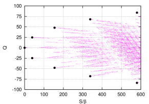
Let us first look at the spectrum of the topological charge for the classical solutions. In figure 1 we present a scatter plot of the action (x-axis) and the topological charge (y-axis) for the classical solutions at (left) and (right). We plot all the solutions in the displayed range without any restrictions666For this calculation was quite time-consuming because there are so many classical solutions. However, the figure looks almost the same even if we restrict the number of blocks in eq. (40) to be e.g., .. We observe the accumulation of solutions with the topological charge close to a multiple integer of . The region of action, for which we obtain only solutions with the topological charge close to a multiple integer of , extends with . This agrees with the argument that led to (46) in the previous section.
The minimum action in each topological sector is achieved by the case, for which eqs. (44) and (45) lead to
| (47) |
at large . Note, however, that there are many solutions with which have an action very close to (47). For solutions with larger action, on the other hand, the topological charge takes quite arbitrary values as expected.
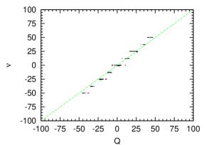
We also observe the accumulation of solutions with the topological charge close to half-integer multiples of . The minimum action achieved by such solutions increases linearly with . These are the solutions having one block with and . By choosing the () so that the arguments of the sine for the other blocks vanish in the large limit, the topological charge (45) becomes
| (48) |
which coincides with the observed spectrum noting that . The action (44) is given by , which nicely explains our observation from figure 1.
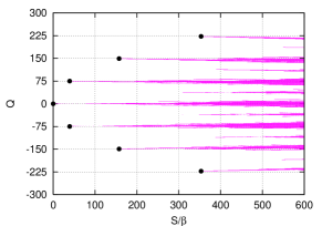
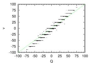
Next let us calculate the index of the overlap Dirac operator for the classical solutions, and examine whether it agrees with the topological charge. In figure 2 we present a scatter plot of the topological charge (x-axis) and the index (y-axis) for solutions at restricting the action in four different regions. We plot all the solutions in the displayed range without any restrictions. For , the index is either or , and the topological charge turns out to be quite close to , which nicely confirms the index theorem. For solutions with larger action, we observe the case with close to half-integer multiples of in accord with (48). While the index theorem is violated to some extent, there still exists a strong correlation between and . It is interesting that the smearing of the pattern occurs mainly in the direction of . In this regard let us recall that the definition (34) of we have used is just a naive descritized version of the continuum formula. In order to recover an exact index theorem in the discretized setting, one may have to use a more sophisticated definition as in the commutative case [47]. Whether this is possible or not is an interesting open question.
5 Configurations with the index of order 1
In the previous section we observed that the topological charge (45) and the index take only multiple integers of for classical solutions with small action. This is in striking contrast to the corresponding commutative theory, where they take arbitrary integers, as we will discuss in section 6. In order to clarify the situation, let us construct configurations with the index of order 1 by interpolating the classical solutions in different topological sectors. This can be achieved by replacing the integer parameters in the explicit form of the classical solutions (43) by real parameters. As the simplest case, we consider the solutions (40) with , and generalize them to a one-parameter family of configurations as
| (49) |
where is a real parameter. Since gives the absolute minimum of the action, it is convenient to define . As a function of , the action and the topological charge can be evaluated as
| (50) | |||||
| (51) |
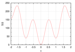
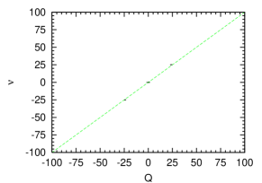
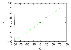
In figure 3 (left) we plot the action against for . Let be the integer which is closest to , and consider the case where with . Then, at large , the leading contribution is given by
| (52) |
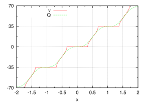
In figure 3 (right) we plot the index of the overlap Dirac operator and the topological charge against for . As we increase from 0 to 1, the index takes various integer values between 0 and . In this way we are able to construct explicit configurations with of order 1. We have also studied , and find that the result of the index is quite stable. For instance, the region of which gives is for , and for . This implies, in view of (52), that the configurations with the index of order 1 constructed above has an action of order .
We also observe in figure 3 (right) that the topological charge does not agree with the index for arbitrary . When is small, we obtain . Therefore, in order to obtain of order 1, we need to have , for which the action becomes of order due to eq. (52). However, for such a small , the index is zero in the large limit according to our discussion in the previous paragraph. This shows that the index theorem is violated even in the large limit if the action is as large as O()777We note that the admissibility condition derived in ref. [61] allows configurations with an action of O(). . It is of course possible that the upper bound on for which the index theorem holds in general is actually less than O(), say O(1). In fact and agree when is close to a half integer, for which becomes of order . We consider this as accidental, however, given the discrepancies observed for configurations with smaller action.
Incidentally, we note that the configurations at (), which gives the local maxima of the action , are closely related to the classical solutions with the topological charge close to half-integer multiples of discussed in the previous section. Indeed, for the two types of configurations, the topological charge as well as the action coincides888Note, however, that they are not exactly equivalent configurations, since the eigenvalue spectrum of is different, and the former type of configuration is actually not a classical solution. at large . In view of this, it is very likely that the classical solutions with the topological charge close to half-integer multiples of actually correspond to saddle-point configurations, instead of being local minima of the action. These solutions are reminiscent of the sphaleron configurations [72].
6 Relationship to the commutative case
In this section we review some known results in the commutative case and discuss their relationship to our results. The commutative counterpart of our theory can be obtained from (7) by replacing the star-product with the ordinary product. The classical solutions are given by configurations with a uniform field strength. Explicitly, such a configuration can be constructed as
| (54) | |||||
| (55) |
where is an integer, which corresponds to the topological charge999A definition of the topological charge in the commutative case can be obtained from (34) by simply replacing the star-product by the ordinary product. This definition gives a non-integer value at finite lattice spacing, and approaches the correct integer value only in the continuum limit. However, there is a simple geometric construction of the topological charge, which gives an integer value even at finite lattice spacing. This definition is used, for instance, in ref. [67]. . In fact one may obtain other solutions by . Since configurations obtained in this way with differing by integers are related with each other by a large gauge transformation, the gauge inequivalent solutions are obtained by restricting within the range . Up to this degeneracy, which corresponds to the moduli space, there is essentially one classical solution in each topological sector labeled by an integer .
For , goes around the unit circle in the complex plane times when goes from 0 to . This implies that the configuration is singular101010Note also that for , while for . Therefore, becomes singular when in the continuum limit. This singularity disappears, however, when is kept finite in the continuum limit or when is a multiple integer of . in the continuum limit with finite since for . (Note, however, that the configuration is physically smooth since the field strength is constant.) This singularity disappears if and only if is a multiple integer of . In that case, the configuration itself becomes totally smooth, and moreover it becomes translationally invariant in the direction 2. For such configurations, the star-product reduces to the ordinary product due to the definition (3). Therefore, the configurations satisfy the star-unitarity condition (8), which implies that they can be thought of as configurations on the discretized 2d NC torus. In fact one can easily show that they correspond to the classical solutions (40) given by a single block ()111111 These configurations have been studied earlier in refs. [68, 69] in the context of gauge theory in commutative space-time.. Note, however, that there are many other classical solutions with larger action in each topological sector on the discretized 2d NC torus.
In the commutative case, the probability distribution of the topological sectors, which are labeled by the index , can be calculated exactly in the continuum121212We thank Hidenori Fukaya for clarification on this point., and it turns out to be , where is the minimum action in the topological sector . In terms of the lattice parameters, may be written as131313For studies of the probability distribution on the lattice, see refs. [67, 70].
| (56) |
at large and . Since in the continuum limit, the distribution scales as a function of , where is the physical extent of the space. Note that the probability for obtaining remains finite.
In the NC case, the classical solutions with the action which is less than of order exist only in the topological sectors labeled by which is a multiple of . The minimum action (47) for classical solutions in these topological sectors agrees with (56) for the reason explained above. In the continuum limit, however, one has to take the limit in such a way that given by (33) is fixed. Since should be sent to infinity as , which follows from the scaling behavior of the correlation functions [18], we obtain finite action only for . This suggests that the probability of obtaining non-zero vanishes in the continuum limit, which is consistent with the instanton calculus in the continuum theory [59]. There the partition function has been written as a sum over all the instanton configurations with the total topological charge constrained to be equal to the magnetic flux, which is zero in the present case.
7 Summary and discussions
In this paper we have studied the index of the overlap Dirac operator in finite NC geometry, and clarified its basic properties including the index theorem. Our results confirm that the overlap Dirac operator indeed captures the topological nature of gauge theory in finite NC geometry, as in commutative lattice gauge theories. An analytic proof of the index theorem extending the works [50] in the commutative case would be an interesting future direction.
In fact we have observed a remarkable impact of NC geometry on the topological properties of the theory. As is well known, we encounter novel topological objects, which are represented by infinitely many classical solutions in each topological sector. However, we also observe the opposite effects. The classical solutions with an action less than of order should have an index which is a multiple integer of . While we were able to construct configurations with the index of order 1 explicitly by interpolating the classical solutions, they have an action of order . The classical solutions with have an action of order 1, but since it is strictly positive and proportional to , the action becomes infinite when one takes the limit. Thus we are left with the sector in the continuum limit141414Repeating our analysis in the case of finite torus would be straightforward, but we consider that the topologically nontrivial configurations would be even more difficult to survive the continuum limit.. Confirmation of this statement in the full quantum theory based on Monte Carlo simulation is reported in a separate paper [73].
The model we studied is the U(1) gauge theory on a discretized 2d NC torus, whose commutative counterpart has been studied extensively in the literature for the reason that it shares many dynamical properties with 4d non-abelian gauge theories. The conclusion that the path integral is dominated by the topologically trivial sector implies that the -term151515The parameter, which appears here, represents the coefficient of the instanton number, and it should not be confused with the representing the noncommutativity of the space-time. is irrelevant unlike in the commutative case [71]. It would be interesting to investigate whether the suppression of non-zero indices is a general feature of gauge theories on NC geometry, which is independent of the space-time dimensionality, the gauge group, the matter content and so on. If the same property holds for the NC version of the standard model, it suggests an exciting possibility that the strong CP problem is naturally solved due to the effects of NC geometry.
Note, however, that 4d gauge theories in NC geometry has problems of its own. Unlike the 2d case studied here, the perturbative vacuum in the 4d case actually has tachyonic instability due to the UV/IR mixing [74, 75, 76, 77, 78, 79]. The system stabilizes by “tachyon condensation”, and finds a stable nonperturbative vacuum [19], in which the Wilson line corresponding to the tachyonic mode acquires a vacuum expectation value. Alternatively, one can stabilize the perturbative vacuum by introducing an appropriate UV cutoff. Although we do not know precisely how we should construct a realistic model at this moment, it is tempting to speculate that the strong CP problem may somehow be related to the physics of string theory origin.
Acknowledgments.
It is our pleasure to thank Hidenori Fukaya, Satoshi Iso, Hikaru Kawai, Yusuke Kimura, Takeshi Morita, Kenji Ogawa and Kentaroh Yoshida for valuable discussions.References
- [1] H.S. Snyder, Quantized space-time, Phys. Rev. 71 (1947) 38.
- [2] A. Connes, Noncommutative geometry, Academic Press, 1990.
- [3] S. Doplicher, K. Fredenhagen and J.E. Roberts, The quantum structure of spacetime at the Planck scale and quantum fields, Commun. Math. Phys. 172 (1995) 187 [hep-th/0303037].
- [4] A. Connes, M. R. Douglas and A. Schwarz, Noncommutative geometry and matrix theory: Compactification on tori, J. High Energy Phys. 02 (1998) 003 [hep-th/9711162].
- [5] H. Aoki, N. Ishibashi, S. Iso, H. Kawai, Y. Kitazawa and T. Tada, Noncommutative Yang-Mills in IIB matrix model, Nucl. Phys. B 565 (2000) 176 [hep-th/9908141].
- [6] N. Seiberg and E. Witten, String theory and non-commutative geometry, J. High Energy Phys. 09 (1999) 032 [hep-th/9908142].
- [7] S. Minwalla, M. van Raamsdonk and N. Seiberg, Noncommutative perturbative dynamics, J. High Energy Phys. 02 (2000) 020 [hep-th/9912072].
- [8] J. Ambjørn, Y.M. Makeenko, J. Nishimura and R.J. Szabo, Finite N matrix models of noncommutative gauge theory, J. High Energy Phys. 11 (1999) 029 [hep-th/9911041]; Nonperturbative dynamics of noncommutative gauge theory, Phys. Lett. B 480 (2000) 399 [hep-th/0002158]; Lattice gauge fields and discrete noncommutative Yang-Mills theory, J. High Energy Phys. 05 (2000) 023 [hep-th/0004147].
- [9] S.S. Gubser and S.L. Sondhi, Phase structure of non-commutative scalar field theories, Nucl. Phys. B 605 (2001) 395 [hep-th/0006119].
- [10] W. Bietenholz, F. Hofheinz and J. Nishimura, Simulating non-commutative field theory, Nucl. Phys. 119 (Proc. Suppl.) (2003) 941 [hep-lat/0209021]; Non-commutative field theories beyond perturbation theory, Fortschr. Phys. 51 (2003) 745 [hep-th/0212258]; Numerical results on the non-commutative model, Nucl. Phys. Proc. Suppl. 129 (2004) 865 [hep-th/0309182]; The non-commutative model, Acta Phys. Polon. B 34 (2003) 4711 [hep-th/0309216]; F. Hofheinz, Field theory on a non-commutative plane, Ph.D thesis, Humboldt University (2003) [hep-th/0403117].
- [11] J. Ambjørn and S. Catterall, Stripes from (noncommutative) stars, Phys. Lett. B 549 (2002) 253 [hep-lat/0209106]; X. Martin, A matrix phase for the scalar field on the fuzzy sphere, J. High Energy Phys. 04 (2004) 077 [hep-th/0402230].
- [12] W. Bietenholz, F. Hofheinz and J. Nishimura, Phase diagram and dispersion relation of the non-commutative model in , J. High Energy Phys. 06 (2004) 042 [hep-th/0404020].
- [13] G.-H. Chen and Y.-S. Wu, Renormalization group equations and the Lifshitz point in non-commutative Landau-Ginsburg theory, Nucl. Phys. B 622 (2002) 189 [hep-th/0110134].
- [14] P. Castorina and D. Zappalà, Nonuniform symmetry breaking in noncommutative theory, Phys. Rev. D 68 (2003) 065008 [hep-th/0303030].
- [15] I. Chepelev and R. Roiban, Renormalization of quantum field theories on noncommutative . I: Scalars, J. High Energy Phys. 05 (2000) 037 [hep-th/9911098].
- [16] T. Eguchi and H. Kawai, Reduction of dynamical degrees of freedom in the large N gauge theory, Phys. Rev. Lett. 48 (1982) 1063.
- [17] A. González-Arroyo and M. Okawa, A twisted model for large lattice gauge theory, Phys. Lett. B 120 (1983) 174; The twisted Eguchi-Kawai model: a reduced model for large N lattice gauge theory, Phys. Rev. D 27 (1983) 2397; T. Eguchi and R. Nakayama, Simplification of quenching procedure for large N spin models, Phys. Lett. B 122 (1983) 59.
- [18] W. Bietenholz, F. Hofheinz and J. Nishimura, A non-perturbative study of gauge theory on a non-commutative plane, J. High Energy Phys. 09 (2002) 009 [hep-th/0203151].
- [19] W. Bietenholz, J. Nishimura, Y. Susaki and J. Volkholz, A non-perturbative study of 4d U(1) non-commutative gauge theory: The fate of one-loop instability, J. High Energy Phys. 10 (2006) 042 [hep-th/0608072]; W. Bietenholz, F. Hofheinz, J. Nishimura, Y. Susaki and J. Volkholz, First simulation results for the photon in a non-commutative space, Nucl. Phys. Proc. Suppl. 140 (2005) 772 [hep-lat/0409059]; W. Bietenholz, A. Bigarini, F. Hofheinz, J. Nishimura, Y. Susaki and J. Volkholz, Numerical results for U(1) gauge theory on 2d and 4d non-commutative spaces, Fortsch. Phys. 53 (2005) 418 [hep-th/0501147]; J. Volkholz, W. Bietenholz, J. Nishimura and Y. Susaki, The scaling of QED in a non-commutative space-time, Proc. Sci. LAT2005 (2005) 264 [hep-lat/0509146].
- [20] W. Bietenholz, F. Hofheinz and J. Nishimura, On the relation between non-commutative field theories at and large N matrix field theories, J. High Energy Phys. 05 (2004) 047 [hep-th/0404179].
- [21] J. Madore, The fuzzy sphere, Class. and Quant. Grav. 9 (1992) 69.
- [22] B. P. Dolan and D. O’Connor, A fuzzy three sphere and fuzzy tori, J. High Energy Phys. 10 (2003) 060 [hep-th/0306231].
- [23] D. O’Connor, Field theory on low dimensional fuzzy spaces, Mod. Phys. Lett. A 18 (2003) 2423.
- [24] H. Grosse, C. Klimcik and P. Presnajder, Towards finite quantum field theory in noncommutative geometry, Int. J. Theor. Phys. 35 (1996) 231 [hep-th/9505175].
- [25] P. Aschieri, J. Madore, P. Manousselis and G. Zoupanos, Dimensional reduction over fuzzy coset spaces, J. High Energy Phys. 04 (2004) 034 [hep-th/0310072].
- [26] R. C. Myers, Dielectric-branes, J. High Energy Phys. 12 (1999) 022 [hep-th/9910053].
- [27] S. Iso, Y. Kimura, K. Tanaka and K. Wakatsuki, Noncommutative gauge theory on fuzzy sphere from matrix model, Nucl. Phys. B 604 (2001) 121 [hep-th/0101102].
- [28] T. Azuma, S. Bal, K. Nagao and J. Nishimura, Nonperturbative studies of fuzzy spheres in a matrix model with the Chern-Simons term, J. High Energy Phys. 05 (2004) 005 [hep-th/0401038].
- [29] T. Azuma, S. Bal, K. Nagao and J. Nishimura, Absence of a fuzzy phase in the dimensionally reduced 5d Yang-Mills-Chern-Simons model, J. High Energy Phys. 07 (2004) 066 [hep-th/0405096]; Perturbative versus nonperturbative dynamics of the fuzzy , J. High Energy Phys. 09 (2005) 047 [hep-th/0506205]; Dynamical aspects of the fuzzy CP2 in the large N reduced model with a cubic term, J. High Energy Phys. 05 (2006) 061 [hep-th/0405277]; K. N. Anagnostopoulos, T. Azuma, K. Nagao and J. Nishimura, Impact of supersymmetry on the nonperturbative dynamics of fuzzy spheres, J. High Energy Phys. 09 (2005) 046 [hep-th/0506062]; T. Azuma, K. Nagao and J. Nishimura, Perturbative dynamics of fuzzy spheres at large N, J. High Energy Phys. 06 (2005) 081 [hep-th/0410263].
- [30] R. Gopakumar, S. Minwalla and A. Strominger, Noncommutative solitons, J. High Energy Phys. 05 (2000) 020 [hep-th/0003160]; J. A. Harvey, P. Kraus and F. Larsen, Exact noncommutative solitons, J. High Energy Phys. 12 (2000) 024 [hep-th/0010060].
- [31] N. Nekrasov and A. Schwarz, Instantons on noncommutative and (2,0) superconformal six dimensional theory, Commun. Math. Phys. 198 (1998) 689 [hep-th/9802068]; A. P. Polychronakos, Flux tube solutions in noncommutative gauge theories, Phys. Lett. B 495 (2000) 407 [hep-th/0007043]; D. J. Gross and N. A. Nekrasov, Dynamics of strings in noncommutative gauge theory, J. High Energy Phys. 10 (2000) 021 [hep-th/0007204]; M. Aganagic, R. Gopakumar, S. Minwalla and A. Strominger, Unstable solitons in noncommutative gauge theory, J. High Energy Phys. 04 (2001) 001 [hep-th/0009142]; D. Bak, Exact multi-vortex solutions in noncommutative Abelian-Higgs theory, Phys. Lett. B 495 (2000) 251 [hep-th/0008204]; D. J. Gross and N. A. Nekrasov, Monopoles and strings in noncommutative gauge theory, J. High Energy Phys. 07 (2000) 034 [hep-th/0005204];
- [32] H. Grosse, C. Klimcik and P. Presnajder, Topologically nontrivial field configurations in noncommutative geometry, Commun. Math. Phys. 178 (1996) 507 [hep-th/9510083]; S. Baez, A. P. Balachandran, B. Ydri and S. Vaidya, Monopoles and solitons in fuzzy physics, Commun. Math. Phys. 208 (2000) 787 [hep-th/9811169]; G. Landi, Projective modules of finite type and monopoles over S2, J. Geom. Phys. 37 (2001) 47 [math-ph/9905014]; A. P. Balachandran and S. Vaidya, Instantons and chiral anomaly in fuzzy physics, Int. J. Mod. Phys. A 16 (2001) 17 [hep-th/9910129]; P. Valtancoli, Projectors for the fuzzy sphere, Mod. Phys. Lett. A 16 (2001) 639 [hep-th/0101189]; H. Steinacker, Quantized gauge theory on the fuzzy sphere as random matrix model, Nucl. Phys. B 679 (2004) 66 [hep-th/0307075]; D. Karabali, V. P. Nair and A. P. Polychronakos, Spectrum of Schroedinger field in a noncommutative magnetic monopole, Nucl. Phys. B 627 (2002) 565 [hep-th/0111249]; U. Carow-Watamura, H. Steinacker and S. Watamura, Monopole bundles over fuzzy complex projective spaces, J. Geom. Phys. 54 (2005) 373 [hep-th/0404130].
- [33] A. P. Balachandran and G. Immirzi, The fuzzy Ginsparg-Wilson algebra: A solution of the fermion doubling problem, Phys. Rev. D 68 (2003) 065023 [hep-th/0301242].
- [34] H. Aoki, S. Iso and K. Nagao, Ginsparg-Wilson relation and ’t Hooft-Polyakov monopole on fuzzy 2-sphere, Nucl. Phys. B 684 (2004) 162 [hep-th/0312199].
- [35] M. B. Green, J. H. Schwarz and E. Witten, Superstring theory, vol. 2, Loop amplitudes, anomalies and phenomenology, Cambridge (1988).
- [36] N. Ishibashi, H. Kawai, Y. Kitazawa and A. Tsuchiya, A large-N reduced model as superstring, Nucl. Phys. B 498 (1997) 467 [hep-th/9612115].
- [37] H. Aoki, S. Iso, H. Kawai, Y. Kitazawa and T. Tada, Space-time structures from IIB matrix model, Prog. Theor. Phys. 99 (1998) 713 [hep-th/9802085].
- [38] T. Hotta, J. Nishimura and A. Tsuchiya, Dynamical aspects of large N reduced models, Nucl. Phys. B 545 (1999) 543 [hep-th/9811220]; J. Ambjorn, K. N. Anagnostopoulos, W. Bietenholz, T. Hotta and J. Nishimura, Large N dynamics of dimensionally reduced 4D SU(N) super Yang-Mills theory, J. High Energy Phys. 07 (2000) 013 [hep-th/0003208]; J. Ambjørn, K. N. Anagnostopoulos, W. Bietenholz, T. Hotta and J. Nishimura, Monte Carlo studies of the IIB matrix model at large N, J. High Energy Phys. 07 (2000) 011 [hep-th/0005147]; J. Nishimura and G. Vernizzi, Spontaneous breakdown of lorentz invariance in IIB matrix model, J. High Energy Phys. 04 (2000) 015 [hep-th/0003223]; Brane world generated dynamically from string type IIB matrices, Phys. Rev. Lett. 85 (2000) 4664 [hep-th/0007022]; Z. Burda, B. Petersson and J. Tabaczek, Geometry of reduced supersymmetric 4D Yang-Mills integrals, Nucl. Phys. B 602 (2001) 399 [hep-lat/0012001]; J. Ambjørn, K. N. Anagnostopoulos, W. Bietenholz, F. Hofheinz and J. Nishimura, On the spontaneous breakdown of Lorentz symmetry in matrix models of superstrings, Phys. Rev. D 65 (2002) 086001 [hep-th/0104260]; J. Nishimura, Exactly solvable matrix models for the dynamical generation of space-time in superstring theory, Phys. Rev. D 65 (2002) 105012 [hep-th/0108070]; K. N. Anagnostopoulos and J. Nishimura, New approach to the complex-action problem and its application to a nonperturbative study of superstring theory, Phys. Rev. D 66 (2002) 106008 [hep-th/0108041]; G. Vernizzi and J. F. Wheater, Rotational symmetry breaking in multi-matrix models, Phys. Rev. D 66 (2002) 085024 [hep-th/0206226]; T. Imai, Y. Kitazawa, Y. Takayama and D. Tomino, Effective actions of matrix models on homogeneous spaces, Nucl. Phys. B 679 (2004) 143 [hep-th/0307007]; J. Nishimura, T. Okubo and F. Sugino, Gaussian expansion analysis of a matrix model with the spontaneous breakdown of rotational symmetry, Prog. Theor. Phys. 114 (2005) 487 [hep-th/0412194]; S. Bal, M. Hanada, H. Kawai and F. Kubo, Fuzzy torus in matrix model, Nucl. Phys. B 727 (2005) 196 [hep-th/0412303]; H. Kaneko, Y. Kitazawa and D. Tomino, Stability of fuzzy S S S2 in IIB type matrix models, Nucl. Phys. B 725 (2005) 93 [hep-th/0506033]; Fuzzy spacetime with SU(3) isometry in IIB matrix model, hep-th/0510263.
- [39] J. Nishimura and F. Sugino, Dynamical generation of four-dimensional space-time in the IIB matrix model, J. High Energy Phys. 05 (2002) 001 [hep-th/0111102]; H. Kawai, S. Kawamoto, T. Kuroki, T. Matsuo and S. Shinohara, Mean field approximation of IIB matrix model and emergence of four dimensional space-time, Nucl. Phys. B 647 (2002) 153 [hep-th/0204240]; H. Kawai, S. Kawamoto, T. Kuroki and S. Shinohara, Improved perturbation theory and four-dimensional space-time in IIB matrix model, Prog. Theor. Phys. 109 (2003) 115 [hep-th/0211272].
- [40] S. Iso and H. Kawai, Space-time and matter in IIB matrix model: Gauge symmetry and diffeomorphism, Int. J. Mod. Phys. A 15 (2000) 651 [hep-th/9903217].
- [41] T. Azuma, S. Bal and J. Nishimura, Dynamical generation of gauge groups in the massive Yang-Mills-Chern-Simons matrix model, Phys. Rev. D 72 (2005) 066005 [hep-th/0504217].
- [42] H. B. Nielsen and M. Ninomiya, Absence of neutrinos on a lattice. 1. proof by homotopy theory, Nucl. Phys. B 185 (1981) 20 [Erratum: Nucl. Phys. B 195 (1982) 541].
- [43] P. H. Ginsparg and K. G. Wilson, A remnant of chiral symmetry on the lattice, Phys. Rev. D 25 (1982) 2649.
- [44] M. Lüscher, Exact chiral symmetry on the lattice and the Ginsparg-Wilson relation, Phys. Lett. B 428 (1998) 342 [hep-lat/9802011].
- [45] F. Niedermayer, Exact chiral symmetry, topological charge and related topics, Nucl. Phys. Proc. Suppl. 73 (1999) 105 [hep-lat/9810026].
- [46] R. Narayanan and H. Neuberger, A construction of lattice chiral gauge theories, Nucl. Phys. B 443 (1995) 305 [hep-th/9411108].
- [47] P. Hasenfratz, Prospects for perfect actions, Nucl. Phys. Proc. Suppl. 63 (1998) 53 [hep-lat/9709110]; P. Hasenfratz, V. Laliena and F. Niedermayer, The index theorem in QCD with a finite cut-off, Phys. Lett. B 427 (1998) 125 [hep-lat/9801021].
- [48] H. Neuberger, Exactly massless quarks on the lattice, Phys. Lett. B 417 (1998) 141 [hep-lat/9707022]; Vector like gauge theories with almost massless fermions on the lattice, Phys. Rev. D 57 (1998) 5417 [hep-lat/9710089]; More about exactly massless quarks on the lattice, Phys. Lett. B 427 (1998) 353 [hep-lat/9801031].
- [49] R. Narayanan and P. M. Vranas, A numerical test of the continuum index theorem on the lattice, Nucl. Phys. B 506 (1997) 373 [hep-lat/9702005]; R. G. Edwards, U. M. Heller and R. Narayanan, The hermitian Wilson-Dirac operator in smooth SU(2) instanton backgrounds, Nucl. Phys. B 522 (1998) 285 [hep-lat/9801015]; T. W. Chiu, The spectrum and topological charge of exactly massless fermions on the lattice, Phys. Rev. D 58 (1998) 074511 [hep-lat/9804016]; S. Chandrasekharan, Ginsparg-Wilson fermions: A study in the Schwinger model, Phys. Rev. D 59 (1999) 094502 [hep-lat/9810007]; T. Fujiwara, A numerical study of spectral flows of Hermitian Wilson-Dirac operator and the index theorem in Abelian gauge theories on finite lattices, Prog. Theor. Phys. 107 (2002) 163 [hep-lat/0012007]; J. B. Zhang, S. O. Bilson-Thompson, F. D. R. Bonnet, D. B. Leinweber, A. G. Williams and J. M. Zanotti, Numerical study of lattice index theorem using improved cooling and overlap fermions, Phys. Rev. D 65 (2002) 074510 [hep-lat/0111060].
- [50] D. H. Adams, Axial anomaly and topological charge in lattice gauge theory with overlap-Dirac operator, Annals Phys. 296 (2002) 131 [hep-lat/9812003]; On the continuum limit of fermionic topological charge in lattice gauge theory J. Math. Phys. 42 (2001) 5522 [hep-lat/0009026].
- [51] D. H. Adams and W. Bietenholz, Axial anomaly and index of the overlap hypercube operator, Eur. Phys. J. C 34 (2004) 245 [hep-lat/0307022].
- [52] Y. Kikukawa and A. Yamada, Weak coupling expansion of massless QCD with a Ginsparg-Wilson fermion and axial U(1) anomaly, Phys. Lett. B 448 (1999) 265 [hep-lat/9806013]; K. Fujikawa, A continuum limit of the chiral Jacobian in lattice gauge theory, Nucl. Phys. B 546 (1999) 480 [hep-th/9811235]; H. Suzuki, Simple evaluation of chiral Jacobian with the overlap Dirac operator, Prog. Theor. Phys. 102 (1999) 141 [hep-th/9812019]; T. W. Chiu and T. H. Hsieh, Perturbation calculation of the axial anomaly of Ginsparg-Wilson fermion, hep-lat/9901011; T. Reisz and H. J. Rothe, The axial anomaly in lattice QED: A universal point of view, Phys. Lett. B 455 (1999) 246 [hep-lat/9903003]; M. Frewer and H. J. Rothe, Universality of the axial anomaly in lattice QCD, Phys. Rev. D 63 (2001) 054506 [hep-lat/0004005]; T. Fujiwara, K. Nagao and H. Suzuki, Axial anomaly with the overlap-Dirac operator in arbitrary dimensions, J. High Energy Phys. 09 (2002) 025 [hep-lat/0208057].
- [53] J. Nishimura and M. A. Vazquez-Mozo, Noncommutative chiral gauge theories on the lattice with manifest star-gauge invariance, J. High Energy Phys. 08 (2001) 033 [hep-th/0107110].
- [54] H. Aoki, S. Iso and K. Nagao, Ginsparg-Wilson relation, topological invariants and finite noncommutative geometry, Phys. Rev. D 67 (2003) 085005 [hep-th/0209223].
- [55] A. P. Balachandran, T. R. Govindarajan and B. Ydri, The fermion doubling problem and noncommutative geometry, Mod. Phys. Lett. A 15 (2000) 1279 [hep-th/9911087]; The fermion doubling problem and noncommutative geometry. II, hep-th/0006216.
- [56] S. Iso and K. Nagao, Chiral anomaly and Ginsparg-Wilson relation on the noncommutative torus, Prog. Theor. Phys. 109 (2003) 1017 [hep-th/0212284].
- [57] H. Aoki, S. Iso, T. Maeda and K. Nagao, Dynamical generation of a nontrivial index on the fuzzy 2-sphere, Phys. Rev. D 71 (2005) 045017 [hep-th/0412052], Erratum : Phys. Rev. D 71 (2005) 069905.
-
[58]
L. Griguolo, D. Seminara and P. Valtancoli, Towards the solution
of noncommutative : Morita equivalence and large--limit,
J. High Energy Phys. 12 (2001) 024 [hep-th/0110293];
A. Bassetto, G. Nardelli and A. Torrielli, Perturbative Wilson loop in two-dimensional non-commutative Yang-Mills theory, Nucl. Phys. B 617 (2001) 308 [hep-th/0107147]; Scaling properties of the perturbative Wilson loop in two-dimensional non-commutative Yang-Mills theory, Phys. Rev. D 66 (2002) 085012 [hep-th/0205210]; L. D. Paniak and R. J. Szabo, Open Wilson lines and group theory of noncommutative Yang-Mills theory in two dimensions, J. High Energy Phys. 05 (2003) 029 [hep-th/0302162]; H. Dorn and A. Torrielli, Loop equation in two-dimensional noncommutative Yang-Mills theory, J. High Energy Phys. 01 (2004) 026 [hep-th/0312047]; J. Ambjorn, A. Dubin and Y. Makeenko, Wilson loops in 2D noncommutative Euclidean gauge theory. I: Perturbative expansion, J. High Energy Phys. 07 (2004) 044 [hep-th/0406187]; A. Bassetto, G. De Pol, A. Torrielli and F. Vian, On the invariance under area preserving diffeomorphisms of noncommutative Yang-Mills theory in two dimensions, J. High Energy Phys. 05 (2005) 061 [hep-th/0503175]; M. Cirafici, L. Griguolo, D. Seminara and R. J. Szabo, Morita duality and noncommutative Wilson loops in two dimensions, J. High Energy Phys. 10 (2005) 030 [hep-th/0506016]. - [59] L. D. Paniak and R. J. Szabo, Instanton expansion of noncommutative gauge theory in two dimensions, Commun. Math. Phys. 243 (2003) 343 [hep-th/0203166].
- [60] L. Griguolo and D. Seminara, Classical solutions of the TEK model and noncommutative instantons in two dimensions, J. High Energy Phys. 03 (2004) 068 [hep-th/0311041].
- [61] K. Nagao, Admissibility condition and nontrivial indices on a noncommutative torus, Phys. Rev. D 73 (2006) 065002 [hep-th/0509034].
- [62] A. González-Arroyo and C. P. Korthals Altes, Reduced model for large N continuum field theories, Phys. Lett. B 131 (1983) 396.
- [63] P. van Baal, Surviving extrema for the action on the twisted SU() one point lattice, Commun. Math. Phys. 92 (1983) 1.
- [64] M. F. Atiyah and I. M. Singer, The index of elliptic operators. 5, Annals Math. 93 (1971) 139.
- [65] K. Y. Kim, B. H. Lee and H. S. Yang, Zero-modes and Atiyah-Singer index in noncommutative instantons, Phys. Rev. D 66 (2002) 025034 [hep-th/0205010].
- [66] A. Sako, Instanton number of noncommutative U(n) gauge theory, J. High Energy Phys. 04 (2003) 023 [hep-th/0209139].
- [67] C. R. Gattringer, I. Hip and C. B. Lang, Quantum fluctuations versus topology: A study in U(1)2 lattice gauge theory, Phys. Lett. B 409 (1997) 371 [hep-lat/9706010].
- [68] L. Giusti, A. González-Arroyo, C. Hoelbling, H. Neuberger and C. Rebbi, Fermions on tori in uniform Abelian fields, Phys. Rev. D 65 (2002) 074506 [hep-lat/0112017].
- [69] J. Kiskis, R. Narayanan and H. Neuberger, Proposal for the numerical solution of planar QCD, Phys. Rev. D 66 (2002) 025019 [hep-lat/0203005].
- [70] W. A. Bardeen, A. Duncan, E. Eichten and H. Thacker, Quenched approximation artifacts: A Study in two-dimensional QED, Phys. Rev. D 57 (1998) 3890 [hep-lat/9705002].
- [71] H. Fukaya and T. Onogi, vacuum effects on the chiral condensation and the meson correlators in the two-flavor massive QED2 on the lattice, Phys. Rev. D 70 (2004) 054508 [hep-lat/0403024]; Lattice study of the massive Schwinger model with term under Luescher’s ‘admissibility’ condition, Phys. Rev. D 68 (2003) 074503 [hep-lat/0305004].
- [72] N. S. Manton, Topology in the Weinberg-Salam theory, Phys. Rev. D 28 (1983) 2019; F. R. Klinkhamer and N. S. Manton, A saddle point solution in the Weinberg-Salam theory, Phys. Rev. D 30 (1984) 2212.
- [73] H. Aoki, J. Nishimura and Y. Susaki, Suppression of topologically nontrivial sectors in gauge theory on 2d non-commutative geometry, hep-th/0604093.
- [74] K. Landsteiner, E. Lopez and M. H. G. Tytgat, Excitations in hot non-commutative theories, J. High Energy Phys. 09 (2000) 027 [hep-th/0006210]; Instability of non-commutative SYM theories at finite temperature, J. High Energy Phys. 06 (2001) 055 [hep-th/0104133].
- [75] C. P. Martin and F. Ruiz Ruiz, Paramagnetic dominance, the sign of the beta function and UV/IR mixing in non-commutative U(1),” Nucl. Phys. B 597 (2001) 197 [hep-th/0007131]; F. Ruiz Ruiz, Gauge-fixing independence of IR divergences in non-commutative U(1), perturbative tachyonic instabilities and supersymmetry, Phys. Lett. B 502 (2001) 274 [hep-th/0012171].
- [76] A. Bassetto, L. Griguolo, G. Nardelli and F. Vian, On the unitarity of quantum gauge theories on noncommutative spaces, J. High Energy Phys. 07 (2001) 008 [hep-th/0105257].
- [77] M. van Raamsdonk, The meaning of infrared singularities in noncommutative gauge theories, J. High Energy Phys. 11 (2001) 006 [hep-th/0110093].
- [78] A. Armoni and E. Lopez, UV/IR mixing via closed strings and tachyonic instabilities, Nucl. Phys. B 632 (2002) 240 [hep-th/0110113].
- [79] Z. Guralnik, R. C. Helling, K. Landsteiner and E. Lopez, Perturbative instabilities on the non-commutative torus, Morita duality and twisted boundary conditions, J. High Energy Phys. 05 (2002) 025 [hep-th/0204037].