Phase Diagram of $\mathcal{N}\,{=}\,4$ Super-Yang-Mills Theory with $R$-Symmetry Chemical Potentials

Abstract:

The phase diagram of large $N_{c}$, weakly-coupled $\mathcal{N}\,{=}\,4$ supersymmetric Yang-Mills theory on a three-sphere with non-zero chemical potentials is examined. In the zero coupling limit, a transition line in the $\mu$-$T$ plane is found, separating a “confined” phase in which the Polyakov loop has vanishing expectation value from a “deconfined” phase in which this order parameter is non-zero. For non-zero but weak coupling, perturbative methods may be used to construct a dimensionally reduced effective theory valid for sufficiently high temperature. If the maximal chemical potential exceeds a critical value, then the free energy becomes unbounded below and no genuine equilibrium state exists. However, the deconfined plasma phase remains metastable, with a lifetime which grows exponentially with $N_{c}$ (not $N_{c}^{2}$). This metastable phase persists with increasing chemical potential until a phase boundary, analogous to a spinodal decomposition line, is reached. Beyond this point, no long-lived locally stable quasi-equilibrium state exists.

The resulting picture for the phase diagram of the weakly coupled theory is compared with results believed to hold in the strongly coupled limit of the theory, based on the AdS/CFT correspondence and the study of charged black hole thermodynamics. The confinement/deconfinement phase transition at weak coupling is in qualitative agreement with the Hawking-Page phase transition in the gravity dual of the strongly coupled theory. The black hole thermodynamic instability line may be the counterpart of the spinodal decomposition phase boundary found at weak coupling, but no black hole tunneling instability, analogous to the instability of the weakly coupled plasma phase is currently known.

1 Introduction

The large $N_{c}$ limit of a gauge theory [1] is a type of classical limit [2], and greatly simplifies the structure of the theory. Generalizing QCD from three to a large number $N_{c}$ of colors may appear to be a drastic modification, but the $N_{c}=\infty$ theory exhibits many qualitative similarities to real QCD [3, 4]. However, there are important differences as well. For example, while real QCD (or any normal theory) can only develop genuine phase transitions in the infinite volume limit, $N_{c}=\infty$ theories may have phase transitions even in finite volume, because the $N_{c}\to\infty$ limit acts as a thermodynamic limit. One well-known example of this type is the Gross-Witten transition in two-dimensional $U(N_{c})$ gauge theories [5].

More recently, large $N_{c}$ gauge theories on a finite radius three-sphere at non-zero temperature have been studied by Sundborg [6], and independently by Aharony et al. [7, 8]. These theories were found to have phase transitions even in the limit of zero gauge coupling. Relevant order parameters include the Polyakov loop and the dependence of free energy on $N_{c}$. In the high temperature phase, the Polyakov loop expectation value is non-zero, the associated center symmetry is spontaneously broken, and the free energy scales as $N_{c}^{2}$ as $N_{c}\to\infty$. In the low temperature phase, the Polyakov loop has vanishing expectation value, the center symmetry is unbroken, and the free energy is order one with respect to $N_{c}$ (i.e., the free energy has a finite $N_{c}\to\infty$ limit). In finite volume one cannot operationally define confinement in terms of the free energy needed to separate a static test quark and antiquark to infinity. Nevertheless, we will refer to these phases as “deconfined” and “confining,” respectively, because the corresponding phases of $SU(N_{c})$ Yang-Mills theory in infinite volume show exactly the same features. The reader should bear in mind that the justification for this terminology comes only from the center symmetry realization and the $N_{c}$ dependence of the free energy.

In this paper we consider $\mathcal{N}\,{=}\,4$ supersymmetric Yang-Mills theory (SYM) with gauge group $SU(N_{c})$, on a three-sphere of radius $R$ and in the presence of non-zero chemical potentials associated with the global $R$-symmetry. Our goal is to understand the phase structure of the theory as a function of both temperature and chemical potential. We will focus on the weakly coupled limit of the theory, but will compare results with those which are believed to hold in the strongly coupled limit of the theory, based on the study of solutions of the dual gravitational theory.

The outline of this paper is as follows. In Section 2, we consider the phase structure of $\mathcal{N}\,{=}\,4$ super-Yang-Mills theory on a sphere with $R$-symmetry chemical potentials, in the limit of zero gauge coupling. Section 3 examines the theory with non-zero but weak coupling in the high temperature regime (i.e., inverse temperature small compared to the radius of the spatial three-sphere). In this regime, we construct a dimensionally reduced effective field theory. We compute terms in the resulting effective action up to fourth order in the scalar fields, and evaluate the complete one-loop scalar field effective potential in the special case where the fields take values in the flat directions of the tree-level potential. Section 4 discusses the resulting high temperature thermodynamics and, in particular, the instability of the theory at sufficiently large chemical potential. We summarize the results of our weak-coupling analysis in Section 5 and compare with strong-coupling results obtained from the dual gravitational theory. Some possible extensions are discussed briefly in Section 6.

Appendix A contains details of the reduction of the zero coupling partition function to the matrix model discussed in Section 2. Appendix B presents the one-loop diagrammatic calculations whose results are summarized in Section 3. Appendix C contains the details of the evaluation of the one-loop scalar field effective potential, using a background field method, when the fields lie along flat directions.

The remainder of this introduction summarizes previous work on the thermodynamics of $\mathcal{N}\,{=}\,4$ super-Yang-Mills theory on a sphere. We begin with strong-coupling results which emerge from the AdS/CFT correspondence (or gauge/string duality). This correspondence, which remains unproven but which has passed a great many consistency checks, originated from the congruence of two apparently different theories: Type IIB supergravity on AdS${}_{5}\times S^{5}$ and large $N_{c}$ $\mathcal{N}\,{=}\,4$ super-Yang-Mills theory [9, 10]. The field theory may be regarded as living on the $\mathbb{R}\times S^{3}$ boundary of AdS₅ space [11]. The correspondence between bulk and boundary spaces extends to more general cases including ones where the boundary is $S^{1}\times S^{3}$. The field theory that lives on this manifold is naturally viewed as a finite temperature field theory, with the temperature equaling the inverse of the $S^{1}$ circumference.

For an $S^{1}\times S^{3}$ boundary, there are two possible bulk geometries. One is (Euclidean signature) AdS${}_{5}/\mathbb{Z}$ with the discrete group $\mathbb{Z}$ acting freely on the AdS space, so the resulting manifold is smooth but topologically nontrivial. This gives rise to two spin structures over the manifold. The other bulk manifold with boundary $S^{1}\times S^{3}$ is the (Euclidean signature) Schwarzschild-AdS black hole. This manifold is topologically trivial, and allows a single spin structure. Thus, the sector of AdS${}_{5}/\mathbb{Z}$ geometry which has the same spin structure as the one in Schwarzschild-AdS may flop into Schwarzschild-AdS by a phase transition. This is the Hawking-Page phase transition [12] and, as argued by Witten [13], the signature of this transition in the dual thermal field theory on $S^{1}\times S^{3}$ should be a confinement/deconfinement phase transition.

Various systems that generalize this idea have also been studied. These include, on the gravity side, the thermodynamics of rotating black holes. A rotation may be given either to the AdS₅ bulk or to the internal $S^{5}$ sphere. The former is the Kerr-AdS black hole and the latter, as seen from the bulk, gives rise to the Reissner-Nordström-AdS (RN-AdS) black hole through the usual Kaluza-Klein mechanism whereby momenta in compact extra dimensions appear as charges in the bulk. It is this latter system which is of interest here.

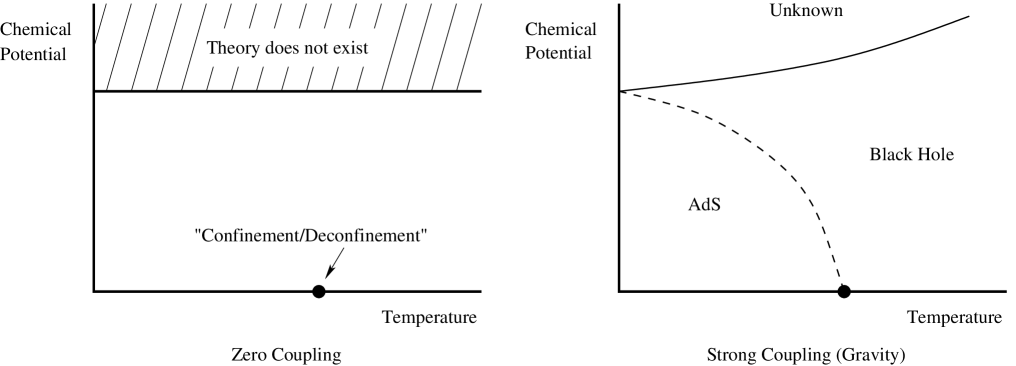
Figure 1: Illustrations of previous results for the phase diagram of $\mathcal{N}\,{=}\,4$ large $N_{c}$ super-Yang-Mills theory as a function of temperature and chemical potential. The left hand figure depicts free field results from the zero coupling limit of the theory while the right hand figure comes from the analysis of the Einstein-Maxwell gravitational system (with three equal charges) which is believed to be dual to the strong coupling limit of the gauge theory.

The action that governs the bulk thermodynamics is the five dimensional Einstein-Maxwell action with negative cosmological constant (and Euclidean signature). This action has two saddle points. One is AdS space without a black hole, the other is the RN-AdS black hole. One may use either the Reissner-Nordström charge, or the associated chemical potential to parameterize these solutions. For the grand canonical ensemble, the relevant parameters are temperature and chemical potential. The equilibrium state of the system corresponds to whichever of the two saddle point configurations minimizes the free energy (which corresponds to the gravity action minus an appropriate boundary term [15, 16]). The resulting phase diagram has a transition line separating these two phases, drawn as the dashed line in the right hand diagram of Fig. 1. This is the generalization of the Hawking-Page phase transition to non-zero charge; the original Hawking-Page transition is indicated in the figure by the dot on the temperature axis at zero chemical potential. This transition between AdS and RN-AdS black hole solutions is a first order phase transition [17].

Cvetic and Gubser analyzed the thermodynamic stability of the black holes [18] and found an instability line in the phase diagram (in addition to the Hawking-Page phase transition line). Beyond the instability line, the black hole that extremizes the Euclidean action becomes a saddle point; this corresponds to a thermodynamic instability. The instability line is indicated by the solid line in the right hand diagram of Fig. 1.

A natural question is the fate of the theory beyond this instability line. For the case of the RN-AdS black hole in four dimensions, Gubser and Mitra [19] found that the instability point is almost exactly where supergravity develops tachyonic modes. (There is 0.7% numerical discrepancy which is believed to be a numerical analysis artifact.) It is generally presumed that the theory enters a new phase beyond the instability line. But in the absence of any explicit solution corresponding to such a putative new phase, it is also possible that this line represents a genuine boundary to the phase diagram, beyond which no equilibrium state exists. This would be analogous to the situation at zero coupling, discussed below. In short, the fate of the theory beyond the instability line is not currently known.

We now turn to previous work on the thermodynamics of weakly coupled $SU(N_{c})$ $\mathcal{N}\,{=}\,4$ super-Yang-Mills theory with non-zero chemical potentials for $R$-charges, in the large $N_{c}$ limit. If one considers the theory on flat space and introduces any non-zero chemical potential, then there is an immediate problem — no ground state (or grand canonical equilibrium state) exists. A chemical potential acts like a negative mass squared for the scalar fields. Due to conformal symmetry, this theory (on flat space) has no mass term. Because there are flat directions in the super-potential, any non-zero chemical potential immediately destabilizes the theory.

Compactifying space by replacing flat $\mathbb{R}^{3}$ with a three-sphere of radius $R$ avoids this problem. The coupling of the scalar fields to the spacetime curvature acts like a positive mass squared and allows one to introduce non-zero chemical potentials, provided they are sufficiently small. In the limit of zero gauge coupling, the maximum chemical potential equals the curvature-induced scalar mass, namely $1/R$. For larger chemical potentials, the theory is again unstable and no equilibrium state exists. Hence, as illustrated on the left in Fig. 1, in the free field theory the line $\mu=1/R$ is a boundary of the phase diagram (just like the $T=0$ line) and is not a phase transition line.

This point of instability has been referred to as “Bose-Einstein condensation” in the AdS/CFT literature (e.g., Refs. [20, 21]) but this is highly mis-leading terminology. In an interacting system, Bose-Einstein condensation corresponds to spontaneous symmetry breaking of a global $U(1)$ symmetry. In a $\mu$-$T$ phase diagram, a Bose-Einstein condensation line is a phase transition line separating distinct phases — it is not a boundary of the phase diagram.

In the free theory on $S^{3}$ without a chemical potential one finds [6, 7], a “confinement/deconfinement” phase transition as the temperature is increased, as noted earlier. This is indicated by the dot on the temperature axis at zero chemical potential on the left side of Fig. 1.

Hawking and Reall [21], considering the free theory on $S^{3}$ with a chemical potential, noted the phase boundary at $\mu=1/R$, but did not find any confinement/deconfinement transition and concluded that the free field theory in this particular system is qualitatively different from the conjectured strongly coupled dual gravity system. However, these authors ignored the constraint of Gauss’ law and the associated requirement that physical states be gauge invariant. It is the restriction to gauge invariant states which is responsible for the confinement/deconfinement transition at vanishing chemical potential [6, 7]. Maintaining Gauss’ law, even at zero coupling, is necessary to obtain valid results for the limiting weak coupling behavior of the interacting theory. In Section 2 we reanalyze the free theory with non-zero chemical potentials and the Gauss law constraint, and show that there is a confinement/deconfinement phase transition line which connects the $\mu=0$, $T\neq 0$ transition point with the zero temperature limit of stability point at $\mu=1/R$ and $T=0$.

From Fig. 1, one may also note differences in the instability/phase-boundary lines. In the strong-coupling gravity dual, the chemical potential grows with temperature on the instability line [18] and at asymptotically high temperatures, the instability line rises linearly. In the free field theory, the limiting chemical potential defining the phase diagram boundary is independent of temperature and, as we show below, is unaffected by the imposition of Gauss’ law. In Section 3 we consider the theory at non-zero but small coupling, and high temperature, and find that a thermal mass is generated in addition to the spatial curvature induced mass. The resulting effective scalar mass (squared) remains positive until one reaches a “spinodal decomposition” line on which the chemical potential also rises linearly at asymptotically high temperatures. This is discussed further in section 4.

As this work was nearing completion, we became aware of the recent work of Basu and Wadia [22], which discusses the canonical emsenble of $\mathcal{N}\,{=}\,4$ super-Yang-Mills theory with fixed $R$-charges, instead of fixed chemical potentials. These authors examined an approximation to the zero coupling limit of the gauge invariant partition function with a projection onto states of a given $R$-charge, and found multiple saddle points with differing (but always non-zero) expectation values for the Polyakov loop. They also constructed a simple model illustrating the effect of turning on a weak coupling, and discussed similarities between their model’s results and properties of $R$-charged anti-de-Sitter black holes. At first sight, the results of Ref. [22] appear quite different from the picture of the $\mathcal{N}\,{=}\,4$ phase diagram which emerges from our analysis. However, as we discuss in Section 2.6, proper consideration of the relation between canonical and grand canonical ensembles near a first order phase transition shows that the qualitative results of Ref. [22] are consistent with our phase structure.

2 Zero Coupling Limit

Consider free $\mathcal{N}\,{=}\,4$ $SU(N_{c})$ supersymmetric Yang-Mills theory on $S^{3}$. This field theory has a global $SU(4)$ $R$-symmetry (denoted $SU(4)_{R}$) and one may introduce chemical potentials coupled to the corresponding conserved charges. It should be emphasized that the “free” gauge theory considered in this section is the zero coupling limit of the theory while retaining Gauss’ law. This is appropriate since Gauss’ law holds and physical states are necessarily gauge invariant at all non-zero values of the coupling. In particular, one must have global charge neutrality of all physical states even with an infinitesimally small coupling constant.

For free gauge theories on a sphere, there are two equivalent techniques for computing the resulting partition function: counting gauge invariant states directly, or using a suitable functional integral representation. The former method, adopted in Refs. [6, 23, 7], takes advantage of the conformal mapping relating operators in the theory on $\mathbb{R}^{4}$ to states of the theory on the sphere. One counts the number of gauge invariant operators of a given dimension (which maps to the energy of the state on the sphere), and then sums over all such operators to obtain the partition function on the sphere.

We choose to employ the functional integral approach (also discussed in Ref. [7]) which represents the projection onto gauge invariant states via an integral over the time component of the gauge field. We begin, in subsection 2.1, by reviewing the introduction of chemical potentials for a maximal Abelian subgroup of a non-Abelian global symmetry group, and then in subsection 2.2 write down the Lagrangian of the theory with the chemical potentials included. Using this Lagrangian, subsection 2.3 presents the matrix model which describes the partition function of the free theory on the sphere. We sketch the derivation of this matrix model, but leave details to Appendix A. The resulting phase diagram for the free theory is discussed in subsection 2.4, and shown to have a phase transition line separating a “confining” low temperature or small chemical potential phase from a “deconfined” high temperature/large chemical potential phase. In the final subsection 2.5 we show that this is a first order phase transition in the zero coupling limit, but note that it is possible for the transition to become continuous at any non-zero coupling.

2.1 Chemical Potentials for Non-Abelian Symmetries

Consider a system with Hamiltonian $\hat{H}$ and internal symmetry group $G$, assumed to be a semi-simple compact Lie group. A Cartan subalgebra of $G$ is also a maximal Abelian subalgebra, with dimension equal to the rank of the group $G$. Compactness implies that any group element may be written as the exponential of some element in the Lie algebra. Let $\hat{U}(g)$ be the unitary operator representing an element $g$ of the group, and define

$$Z(\beta,g)=\operatorname{tr}\,[\hat{U}(g)e^{-\beta\hat{H}}]\;,$$ (1)

where $\beta$ is the inverse temperature. By assumption, $\hat{U}(g)$ commutes with $\hat{H}$ for all group elements $g$. Consequently $Z(\beta,g)$ is a class function since (using trace cyclicity),

$$Z(\beta,g)=\operatorname{tr}\,[\hat{U}(\eta)\,\hat{U}(g)\,\hat{U}(\eta)^{-1}e^{-\beta H}]=\operatorname{tr}\,[\hat{U}(\eta g\eta^{-1})\,e^{-\beta H}]=Z(\beta,\eta g\eta^{-1})\;,$$ (2)

for arbitrary $\eta$ in $G$. Any group element $g$ is equivalent (under conjugation by group elements) to some element $h$ of a maximal Abelian subgroup. And any element of a maximal Abelian subgroup may be expressed as an exponential of a sum of generators of a Cartan subalgebra, $h=e^{i\gamma_{p}\hat{Q}_{p}}$ where $\{\hat{Q}_{p}\,|\,p{=}1,\cdots,\operatorname{rank}(G)\}$ are the generators and $\{\gamma_{p}\}$ are real numbers. We are adopting the convention that the generators $\{\hat{Q}_{p}\}$ are Hermitian. Therefore, $Z(\beta,g)$ may be regarded as a function of the $\operatorname{rank}(G)$ real variables $\{\gamma_{p}\}$, and rewritten as

$$Z(\beta,\gamma_{p})=\operatorname{tr}\,e^{-\beta\hat{H}}e^{i\gamma_{p}\hat{Q}_{p}}\;.$$ (3)

After an analytic continuation $\gamma_{p}\rightarrow-i\beta\mu_{p}$, this is the grand canonical partition function

$$Z(\beta,\mu_{p})\equiv\operatorname{tr}\,\exp[-\beta(\hat{H}-\mu_{p}\,\hat{Q}_{p})]\;,$$ (4)

with chemical potentials $\{\mu_{p}\}$ associated with a maximal set of commuting conserved charges $\{\hat{Q}_{p}\}$. This illustrates why, given a non-Abelian symmetry group, it is natural to introduce chemical potentials corresponding to a Cartan subalgebra of the group.

2.2 $\mathcal{N}\,{=}\,4$ Super-Yang-Mills Lagrangian with Chemical Potentials

Four dimensional $\mathcal{N}\,{=}\,4$ super-Yang-Mills theory, in flat space, may be obtained from dimensional reduction of ${\cal N}\,{=}\,1$ super-Yang-Mills in ten dimensions [25, 26]. We consider this theory on $S^{1}\times S^{3}$, and include chemical potentials associated with a $U(1)^{3}$ maximal Abelian subgroup of the $SU(4)$ global $R$-symmetry. As mentioned in the Introduction, this theory has conformal scalar-curvature coupling terms that will appear as mass terms for the scalar fields.

To write the Lagrangian, we first determine how the charges $\hat{Q}_{p}$ associated with the chemical potentials transform each field of the theory. The field content includes six scalars which we will regard as components of an antisymmetric matrix, $\phi_{ij}$ ($i,j=1,\ldots,4$) with $\phi_{ij}=-\phi_{ji}$, four (left-handed) Weyl fermions $\lambda_{i}$, and a vector field $A_{\nu}$, all transforming in the adjoint representation of the gauge group $SU(N_{c})$.

The scalar fields $\phi_{ij}$ are complex, and transform under the antisymmetric representation $\mathbf{6}$ of $SU(4)_{R}$. One may repackage these fields as a $\bar{\mathbf{6}}$, defined by

$$\phi^{ij}\equiv{\textstyle\frac{1}{2}}\,\epsilon^{ijkl}\,\phi_{kl}\;.$$ (5)

Since the $\bar{\mathbf{6}}$ representation is the complex conjugate of the $\mathbf{6}$, it is consistent to impose the reality condition $\phi^{ij}=\phi_{ij}^{*}$. More explicitly, this is

$$\phi_{12}=\phi_{34}^{*}\;,\quad\phi_{13}=\phi_{42}^{*}\;,\quad\phi_{14}=\phi_{23}^{*}\;,$$ (6)

and the reality constraint leaves six (times $N_{c}^{2}-1$) real degrees of freedom in the scalar fields. To simplify later expressions, we will relabel the three independent complex scalar fields as

$$\phi_{1}\equiv\phi_{12}\,,\qquad\phi_{2}\equiv\phi_{13}\,,\qquad\phi_{3}\equiv\phi_{14}\,.$$ (7)

The counting of degrees of freedom, along with transformation properties under the global $SU(4)_{R}$ symmetry, are summarized in Table 1. Note that the total number of degrees of freedom for bosons and fermions are equal, as usual in supersymmetric theories.

Field D.O.F. $SU(4)_{R}$ $\phi_{p}$ $6\,(N_{c}^{2}{-}1)$ $\mathbf{6}$ $\lambda_{i}$ $8\,(N_{c}^{2}{-}1)$ $\mathbf{4}$ $A_{\nu}$ $2\,(N_{c}^{2}{-}1)$ $\mathbf{1}$

Table 1: Counting of real degrees of freedom, and $SU(4)_{R}$ symmetry representations, for the fields of $\mathcal{N}\,{=}\,4$ super-Yang-Mills theory.

We choose to represent the generators of the Cartan subalgebra, in the fundamental representation $\mathbf{4}$, as

$$Q^{\mathbf{4}}_{1} ={\textstyle\frac{1}{2}}\operatorname{diag}(1,1,-1,-1)\;,$$ (8a)

$$Q^{\mathbf{4}}_{2} ={\textstyle\frac{1}{2}}\operatorname{diag}(1,-1,1,-1)\;,$$ (8b)

$$Q^{\mathbf{4}}_{3} ={\textstyle\frac{1}{2}}\operatorname{diag}(1,-1,-1,1)\;.$$ (8c)

To obtain the corresponding form in the antisymmetric representation $\mathbf{6}$, one may consider the transformations of a rank-2 tensor under $\mathbf{4}\otimes\mathbf{4}$. Assembling the six scalars into a six-component vector via

$$\phi^{T}\equiv(\phi_{1},\phi_{1}^{*},\phi_{2},\phi_{2}^{*},\phi_{3},\phi_{3}^{*})^{T}\,,$$ (9)

the Cartan generator matrices in this representation appear as

$$Q^{\mathbf{6}}_{1} =\operatorname{diag}(1,-1,0,0,0,0)\;,$$ (10a)

$$Q^{\mathbf{6}}_{2} =\operatorname{diag}(0,0,1,-1,0,0)\;,$$ (10b)

$$Q^{\mathbf{6}}_{3} =\operatorname{diag}(0,0,0,0,1,-1)\;.$$ (10c)

With these choices, one sees that

$$\sum_{p=1}^{3}\>\mu_{p}\,Q_{p}^{\mathbf{6}}=\operatorname{diag}(\mu_{1},-\mu_{1},\mu_{2},-\mu_{2},\mu_{3},-\mu_{3})\;.$$ (11)

Hence, $\sum_{p=1}^{3}\mu_{p}\,\hat{Q}_{p}$ assigns eigenvalue $+\mu_{p}$ to $\phi_{p}$ and assigns $-\mu_{p}$ to the complex conjugates $\phi_{p}^{*}$. For the fermions, $\sum_{p=1}^{3}\mu_{p}\,Q_{p}^{\mathbf{4}}=\operatorname{diag}(\tilde{\mu}_{1},\tilde{\mu}_{2},\tilde{\mu}_{3},\tilde{\mu}_{4})$ with

$$\tilde{\mu}_{1}\equiv{\textstyle\frac{1}{2}}(\mu_{1}+\mu_{2}+\mu_{3}),\phantom{-}\quad\tilde{\mu}_{2}\equiv{\textstyle\frac{1}{2}}(\mu_{1}-\mu_{2}-\mu_{3}),\;$$ (12a)

$$\tilde{\mu}_{3}\equiv{\textstyle\frac{1}{2}}(-\mu_{1}+\mu_{2}-\mu_{3}),\quad\tilde{\mu}_{4}\equiv{\textstyle\frac{1}{2}}(-\mu_{1}-\mu_{2}+\mu_{3}),\;$$ (12b)

so the fermion $\lambda_{j}$ has an effective chemical potential $\tilde{\mu}_{j}$.

To derive the correct form of the action to use in a functional integral when chemical potentials are present, one could start from the Lagrangian without chemical potentials, find the conserved charges of the global symmetry, re-express these in terms of conjugate momenta, use this to derive a Hamiltonian path integral representation of the grand canonical partition function (4), and then integrate out the conjugate momenta. But that is completely unnecessary. It is equivalent, but simpler, to imagine gauging the $U(1)^{3}$ Abelian global $R$-symmetry. The time component of such a fictitious gauge field couples to the conserved $U(1)^{3}$ $R$-charge densities, just like the chemical potentials. But the time component of a gauge field in a Euclidean functional integral corresponds to $i$ times the Minkowski gauge potential. Consequently, in a Euclidean functional integral, adding chemical potentials is exactly equivalent to turning on a constant imaginary value for the time component of a background gauge field associated with the $U(1)^{3}$ global $R$-symmetry. One ends up with a standard Euclidean functional integral in which the Lagrangian contains modified covariant derivatives for the time direction,

$$D_{\nu}\rightarrow D_{\nu}-\mu_{p}\,Q_{p}\,\delta_{\nu 0}\;.$$ (13)

It will be convenient for later use to rewrite the Weyl fermions as Majorana fermions. Recall that a massless two-component Weyl fermion $\lambda$, in four dimensions, may be converted to a four-component Majorana fermion $\psi\equiv\binom{\lambda_{\alpha}}{\bar{\lambda}^{\dot{\alpha}}}$. The corresponding terms in the Lagrange density are related via

$$\lambda^{\alpha}\,(\tau_{\nu})_{\alpha\dot{\beta}}\,(\stackrel{{\scriptstyle\leftrightarrow}}{{D}}_{\nu}-\tilde{\mu}\,\delta_{\nu,0})\,\bar{\lambda}^{\dot{\beta}}={\textstyle\frac{1}{2}}\,\bar{\psi}\,({D}\negthickspace{\negthickspace{/}}-\tilde{\mu}\,\gamma_{0}\gamma_{5})\,\psi\;,$$ (14)

where we have defined $\bar{\psi}\equiv(\lambda^{\alpha},\bar{\lambda}_{\dot{\alpha}})$ and

$$\tau_{\nu} \equiv(\mathbf{1},\,i\vec{\sigma})\;,\qquad\bar{\tau}_{\nu}\equiv(\mathbf{1},-i\vec{\sigma})\;,$$ (15a)

$$\gamma_{\nu} \equiv\begin{pmatrix}0&\tau_{\nu}\\ \bar{\tau}_{\nu}&0\end{pmatrix}\,,\quad\gamma_{5}\equiv\gamma_{0}\gamma_{1}\gamma_{2}\gamma_{3}=\begin{pmatrix}\,\mathbf{1}&\phantom{-}0\,\\ \,0&-\mathbf{1}\,\end{pmatrix}.$$ (15b)

The Majorana spinors satisfy the condition

$$\psi=C\bar{\psi}\;,$$ (16)

where $C=\left(\genfrac{}{}{0.0pt}{}{\epsilon_{\alpha\beta}}{0}\genfrac{}{}{0.0pt}{}{0}{\epsilon^{\dot{\alpha}\dot{\beta}}}\right)$ is the charge conjugation matrix with $\epsilon_{12}=-\epsilon_{21}\equiv-1$.

The gauge field $A_{\mu}$ may be regarded as a traceless Hermitian matrix. Equivalently, it may be expanded as $A_{\mu}=A_{\mu}^{a}\,T^{a}$, with real coefficients $\{A_{\mu}^{a}\}$ and Hermitian color generators $T^{a}$ which satisfy

$$[T^{a},T^{b}] =if^{abc}\,T^{c}\;,$$ (17a)

and

$$\operatorname{tr}\,(T^{a}T^{b}) ={\textstyle\frac{1}{2}}\,\delta^{ab}\;.$$ (17b)

With this choice, the structure constants $f^{abc}$ are real and completely antisymmetric.

The scalar and fermion fields may similarly be expanded in the basis of color generators, $\phi_{p}=\phi_{p}^{a}\,T^{a}$ and $\psi_{i}=\psi_{i}^{a}\,T^{a}$. The coefficient $\psi_{i}^{a}$ is a four-component Grassmann-valued spinor. The conjugate spinor $\bar{\psi}_{i}^{a}$ is not independent, but is related to $\psi_{i}^{a}$ via the Majorana condition (16). The coefficients $\phi_{p}^{a}$ satisfy the reality condition (6) (for each $a$). It will be convenient to introduce explicitly independent real scalar fields via $\phi_{p}\equiv(X_{p}+iY_{p})/\sqrt{2}$ and to assemble these into a multiplet,

$$\Phi\equiv(X_{1},Y_{1},X_{2},Y_{2},X_{3},Y_{3})\;.$$ (18)

We will use a capital Latin index to denote components of this vector, so $\Phi_{A}=\Phi_{A}^{a}\,T^{a}$ with $A=1,\cdots,6$.

We are finally ready to write down the $\mathcal{N}=4$ SYM Lagrange density [25, 26] in Euclidean signature with the addition of chemical potentials and spatial curvature induced mass terms:

$$\mathcal{L}= \operatorname{tr}\,\Bigl{\{}{\textstyle\frac{1}{2}}(F_{\mu\nu})^{2}+(D_{\nu}X_{p}-i\mu_{p}\,\delta_{\nu,0}Y_{p})^{2}+(D_{\nu}Y_{p}+i\mu_{p}\,\delta_{\nu,0}X_{p})^{2}+R^{-2}\,(\Phi_{A})^{2}$$

$$+i\bar{\psi}_{i}({D}\negthickspace{\negthickspace{/}}-\tilde{\mu}_{i}\,\gamma_{0}\gamma_{5})\psi_{i}+{\textstyle\frac{1}{2}}\,g^{2}(i[\Phi_{A},\Phi_{B}])^{2}-g\,\bar{\psi}_{i}\left[(\alpha^{p}_{ij}X_{p}+i\beta^{q}_{ij}\gamma_{5}Y_{q}),\,\psi_{j}\right]\Bigr{\}}\,,$$ (19)

where $F_{\mu\nu}=\partial_{\mu}A_{\nu}-\partial_{\nu}A_{\mu}+ig[A_{\mu},A_{\nu}]$ and $D_{\nu}=\partial_{\nu}+ig[A_{\nu},\,\cdot\,]$. The indices run over $A,B=1,\cdots\!,6$, $p,q=1,\cdots\!,3$, $i,j=1,\cdots\!,4$, and $a=1,\cdots\!,N_{c}^{2}-1$ (with implied sums over all indices). The $4\times 4$ matrices $\alpha^{p}$ and $\beta^{q}$ satisfy the relations

$$\{\alpha^{p},\alpha^{q}\}=-2\,\delta^{pq}\,\mathbf{1}_{4\times 4}\;,\quad\{\beta^{p},\beta^{q}\}=-2\,\delta^{pq}\,\mathbf{1}_{4\times 4}\;,\quad[\alpha^{p},\beta^{q}]=0\;,$$ (20)

and explicit forms can be given as

$$\alpha^{1} =\begin{pmatrix}0&\sigma_{1}\\ -\sigma_{1}&0\end{pmatrix},\;\alpha^{2}=\begin{pmatrix}0&-\sigma_{3}\\ \sigma_{3}&0\end{pmatrix},\;\alpha^{3}=\begin{pmatrix}i\sigma_{2}&0\\ 0&i\sigma_{2}\end{pmatrix},\;$$ (21a)

$$\beta^{1} =\begin{pmatrix}0&i\sigma_{2}\\ i\sigma_{2}&0\end{pmatrix},\;\beta^{2}=\begin{pmatrix}0&\sigma_{0}\\ -\sigma_{0}&0\end{pmatrix},\;\beta^{3}=\begin{pmatrix}-i\sigma_{2}&0\\ 0&i\sigma_{2}\end{pmatrix}\,.$$ (21b)

The partition function for the grand canonical ensemble has the functional integral representation

$$Z=\int{\cal D}A_{\mu}\>{\cal D}\psi_{i}\>{\cal D}\Phi_{A}\;e^{-\textstyle\!\int d^{4}x\>{\cal L}}\,,$$ (22)

where the integral is over fields taking values on $S^{3}$ (of radius $R$)${}\times S^{1}$ (of radius $\beta$), with the gauge and scalar fields periodic and the Grassmann-valued fermion fields anti-periodic on the Euclidean time circle.

2.3 Gauge Invariant Partition Function

We want to compute the partition function (22) in the free-field limit of the theory, while preserving the projection onto gauge invariant states which is embodied in the functional integral over $A_{0}$. We sketch the calculation here, and leave details to Appendix A.

Taking a naive $g\to 0$ limit of the Lagrangian (2.2) is the wrong procedure; this ignores the special role of $A_{0}$ as a Lagrange multiplier enforcing Gauss’ law and, as detailed below, would lead to an ill-defined Gaussian integral due to a zero-mode in the covariance operator for $A_{0}$. The physically appropriate limit is obtained by sending $g\to 0$ after separating and rescaling the constant mode of $A_{0}$,

$$A_{0}(x)\longrightarrow\tilde{A}_{0}(x)+a/g\,,$$ (23)

with $\tilde{A}_{0}(x)$ constrained to have a vanishing spacetime integral, and $a$ an arbitrary traceless $N_{c}\times N_{c}$ Hermitian constant matrix. The net effect is that the $g=0$ functional integral includes configurations in which parallel transporters around the time circle, $U\equiv{\cal P}\,(e^{ig\int_{0}^{\beta}dx^{0}\>A_{0}})$, cover the entire gauge group. It is the resulting integration over $U$ which implements the projection onto gauge invariant states. After suitably fixing a gauge, the remaining functional integral is a well-defined Gaussian integral over all degrees of freedom other than $a$, the constant mode of $A_{0}$, and a non-Gaussian integral over the single matrix $a$.

The Gaussian integral leads to functional determinants of the covariance (or small fluctuation) operators defined by the quadratic part of the action. For the scalar fields, this operator involves the sum of the square of a covariant time derivative, which depends on $a$ and the chemical potentials, a spatial Laplacian, and the curvature-induced mass term. The gauge field covariance operator and the square of the fermion operator have completely analogous forms, but with the relevant Laplacian acting on vector or spinor fields, respectively, and without any mass term. Eigenfunctions of these operators are exponentials in time, $e^{i\omega_{k}t}$, multiplied by scalar, vector, or spinor $S^{3}$-spherical harmonics. The frequencies $\omega_{k}$ are quantized Matsubara frequencies, and equal $2k\pi/\beta$ for bosons and $(2k{+}1)\pi/\beta$ for fermions. The eigenvalues of the Laplacian on the three-sphere may be regarded as squares of discrete spatial momenta, and scale as $1/R^{2}$, where $R$ is the radius of the sphere. We will generally set $R=1$, and assume all momenta and energies are measured in the units of $1/R$.

field eigenvalue degeneracy transverse vector ${\bf A}_{\perp}$ $(h+1)^{2}$ $2h\,(h+2)$ longitudinal vector $\nabla F$ $h\,(h+2)$ $(h+1)^{2}$ real scalar $A_{0}$ $h\,(h+2)$ $(h+1)^{2}$ conformal scalar $\Phi_{A}$ $(h+1)^{2}$ $(h+1)^{2}$ Majorana spinor $\psi_{i}$ $(h+{\textstyle\frac{1}{2}})^{2}$ $h\,(h+1)$

Table 2: Eigenvalues (in units of $1/R^{2}$) and degeneracies of the spatial part of the small fluctuation operator for scalar, spinor, and vector fields. The relevant operator is just the Laplacian on $S^{3}$ for all fields except conformally coupled scalars, where it includes a shift by $1/R^{2}$ due to the curvature induced mass term. Representations of the $SO(4)$ isometry group are labeled by $h=0,1,2,\cdots$, except for the longitudinal vector $\nabla F$, where $h$ starts from 1.

The eigenvalues and associated degeneracies of the spatial part of the small fluctuation operator, equal to the spatial Laplacian plus the mass term (for scalars), are shown in Table 2. Representations of the $SO(4)$ isometry group are labeled by the integer $h$ which runs over all non-negative values; $h/R$ may be regarded as a discrete spatial momentum. The degeneracy factors are the dimension of the representations at each value of $h$. Spatial components of the gauge fields have been decomposed into a transverse (i.e., divergenceless) vector field ${\bf A}_{\perp}$ and a gradient of a scalar, $\nabla F$. The longitudinal vector $\nabla F$ vanishes for constant $F$, and therefore $h$ starts from $1$ in this case. The spatial small fluctuation operator for the conformally coupled scalar fields $\Phi_{A}$ includes their curvature induced mass term, so their eigenvalues are $h(h+2)+1=(h+1)^{2}$. The time component of the gauge field, $A_{0}$, is a scalar with respect to the $SO(4)$ isometry and has no mass. Note that only $A_{0}$ has a zero eigenvalue and its associated eigenfunction is constant on $S^{3}$. The lack of zero modes for divergenceless vector and spinor fields is due to the topology of $S^{3}$, which cannot support constant tensors of rank higher than zero.

The complete small fluctuation eigenvalues equal these spatial eigenvalues plus the square of a Matsubara frequency shifted by an amount proportional to a difference of eigenvalues of the matrix $a$ and (for scalars and fermions) by $i$ times a chemical potential. Details are given in Appendix A. For the scalar fields $\Phi_{A}$, the complete small fluctuation eigenvalues are

$$(\omega_{k}+q_{m}-q_{n}\pm i\mu_{p})^{2}+(h+1)^{2}\,,$$ (24)

where $\{q_{n}\}$ are the real eigenvalues of $a$, $\omega_{k}=2\pi k/\beta$, $m,n=1,\cdots,N_{c}$, and $h=0,1,\cdots$. Note that if the magnitude of the chemical potential $\mu_{p}$ exceeds unity (times $1/R$) then, for $m=n$ and $h=k=0$, the real part of the eigenvalue (24) becomes negative — which means that the Gaussian integral fails to be well-defined. This can be seen directly from the Lagrangian (2.2), which shows that non-zero chemical potentials act like a negative mass squared for static diagonal components of the scalar field $\Phi_{A}$. If the chemical potential exceeds the $1/R$ curvature induced mass, then the Euclidean action becomes unbounded below and the partition function ceases to exist. So $|\mu_{p}|=1/R$ represents a boundary of the phase diagram of the free theory. In the remainder of this section we assume all chemical potentials are less than $1/R$ (in magnitude).

The small fluctuation operator for the static (zero frequency) component of $A_{0}$ has no temporal contribution and is just the scalar Laplacian on $S^{3}$. The presence of a zero eigenvalue of the small fluctuation operator for $A_{0}$ illustrates the necessity for separating the constant mode of $A_{0}$ from the other degrees of freedom, as done in (23). The contributions from the non-constant part of $A_{0}$ and the longitudinal part of the spatial gauge field, $\nabla F$, end up canceling the contributions from gauge-fixing ghosts (which are also scalars with respect to $SO(4)$). The logarithms of the resulting functional determinants involve a sum over all Matsubara frequencies and a sum over the discrete momentum $h$ labeling $S^{3}$ spherical harmonics. As shown in Appendix A, the Matsubara sum may be performed explicitly and the result for the logarithm of the Gaussian integral may be cast in the form of an effective action for the single $SU(N_{c})$ matrix $U\equiv\exp(i\beta a)$,

$$S_{\rm eff}(U)=-\sum_{n=1}^{\infty}\frac{1}{n}\left\{z_{B}(x^{n})+(-1)^{n+1}z_{F}(x^{n})\right\}[\operatorname{tr}(U^{n})\operatorname{tr}(U^{\dagger n})-1]\;,$$ (25)

where $x\equiv e^{-\beta}=e^{-1/T}$ and we have defined the “single particle” partition functions:

$$z_{B}(x) \equiv z_{S}(x)+z_{V}(x)\,,$$ (26a)

$$z_{V}(x) \equiv\frac{6x^{2}-2x^{3}}{(1-x)^{3}}\,,$$ (26b)

$$z_{S}(x) \equiv\frac{x+x^{2}}{(1-x)^{3}}\left(x^{\mu_{1}}+x^{-\mu_{1}}+x^{\mu_{2}}+x^{-\mu_{2}}+x^{\mu_{3}}+x^{-\mu_{3}}\right)\,,$$ (26c)

$$z_{F}(x) \equiv\frac{2x^{3/2}}{(1-x)^{3}}\,\bigl{(}x^{\frac{1}{2}\mu_{1}}+x^{-\frac{1}{2}\mu_{1}}\bigr{)}\bigl{(}x^{\frac{1}{2}\mu_{2}}+x^{-\frac{1}{2}\mu_{2}}\bigr{)}\bigl{(}x^{\frac{1}{2}\mu_{3}}+x^{-\frac{1}{2}\mu_{3}}\bigr{)}\,.$$ (26d)

To obtain the grand canonical partition function, we must integrate over the remaining single matrix $a$, or equivalently over the group element $U$,

$$Z(x)=\int dU\>\exp[-S_{\rm eff}(U)]\;.$$ (27)

The required measure $dU$ is Haar measure on the group $SU(N_{c})$. Even though we have derived the matrix model (25)–(27) specifically for $\mathcal{N}\,{=}\,4$ $SU(N_{c})$ SYM theory, the model dependence is only in the specific field content and group character. The generalization to other gauge theories in the zero coupling limit is straightforward.

2.4 Phase Structure of the Free Theory

The reduced theory (27) is a single matrix model. In the large $N_{c}$ limit, this can be solved in a manner similar to the Gross-Witten model [5]. The required analysis is a straightforward generalization of the zero chemical potential case discussed in Refs. [7, 6]. Hence we will only sketch the procedure; interested readers should refer to Refs. [7, 6] for details.

After rewriting the integration measure in terms of the eigenvalues of $U$, and introducing the eigenvalue distribution function, $\rho(\theta)$, one arrives at the following form of the effective action for the eigenvalue distribution,

$$S_{\rm eff}[\rho]=N_{c}^{2}\sum_{n=1}^{\infty}\>V_{n}\,\rho_{n}^{2}\;,$$ (28)

where $\rho_{n}\equiv\int_{-\pi}^{\pi}d\theta\,\rho(\theta)\cos(n\theta)$ are the Fourier series coefficients of the eigenvalue distribution, and

$$V_{n}\equiv\frac{1}{n}\left\{1-\left[z_{B}(x^{n})+(-1)^{n+1}\,z_{F}(x^{n})\right]\right\}\;.$$ (29)

The factor of $N_{c}^{2}$ multiplying the effective action (28) implies that the minimum value of this effective action determines the leading large $N_{c}$ behavior of the free energy $F\equiv-\beta^{-1}\ln Z$, with fluctuations in the eigenvalue density only generating subleading $\mathcal{O}(N_{c}^{0})$ contributions to the free energy. As $N_{c}\to\infty$,

$$F=\mathop{\min}\limits_{\{\rho\}}\>\frac{S_{\rm eff}[\rho]}{\beta}+\mathcal{O}(N_{c}^{0})\,.$$ (30)

In the effective action (28) each positive $V_{n}$ acts as a repulsive potential for the eigenvalue distribution, while negative $V_{n}$’s act as attractive potentials. Thus the condition

$$z_{B}(x^{n})+(-1)^{n+1}z_{F}(x^{n})<1$$ (31)

ensures that all $V_{n}$ are positive and implies that the system is in the phase where eigenvalues repel and the uniform distribution $\rho(\theta)=\frac{1}{2\pi}$ characterizes the equilibrium state. As long as all $|\mu_{p}|$ are less than one, which is required for the existence of the grand canonical ensemble, it is easy to see that our modified single particle partition functions (26) increase monotonically with $x$. Hence, the $n=1$ term in the inequality (31) gives the most stringent condition. Therefore, the curve in the $\mu$-$T$ diagram determined by the threshold condition

$$z_{B}(x)+z_{F}(x)=1$$ (32)

gives the boundary of the phase in which the eigenvalue distribution is uniform and $\operatorname{tr}(U^{n})$ has vanishing expectation value (for all $n\neq 0$).

In the free-field and large $N_{c}$ limit, the Polyakov loop expectation value is just $\rho_{1}$:

$$\left\langle{\textstyle\frac{1}{N_{c}}}\operatorname{tr}\,{\cal P}\left(e^{ig\int_{0}^{\beta}dx^{0}\>A_{0}}\right)\right\rangle=\left\langle{\textstyle\frac{1}{N_{c}}}\operatorname{tr}e^{i\beta a}\right\rangle=\left\langle{\textstyle\frac{1}{N_{c}}}\operatorname{tr}U\right\rangle=\int_{-\pi}^{\pi}d\theta\>\rho(\theta)\,e^{i\theta}=\rho_{1}\,.$$ (33)

So in the disordered phase, where the eigenvalues of $U$ are uniformly distributed on the unit circle, the Polyakov loop expectation vanishes. In the ordered phase, where the eigenvalue distribution is non-uniform, the Polyakov loop will have a non-zero expectation value. The Polyakov loop transforms non-trivially under the $\mathbb{Z}_{N_{c}}$ center of the gauge group, and its expectation value is an order parameter for the realization of this symmetry. Thus the $\mathbb{Z}_{N_{c}}$ symmetry is unbroken in the disordered phase, and spontaneously broken in the ordered phase. As emphasized in the Introduction, it is this behavior of the Polyakov loop and the associated realization of the $\mathbb{Z}_{N_{c}}$-symmetry which motivates calling the disordered phase “confining” and the ordered phase “deconfined”.

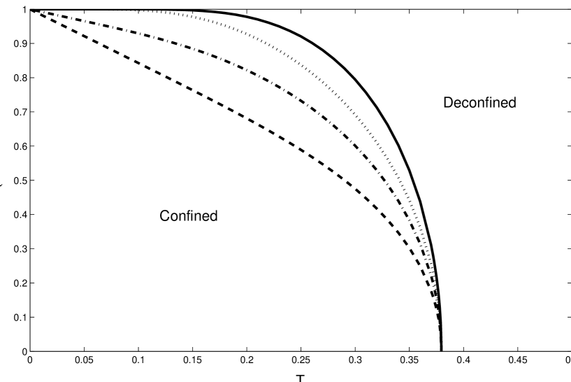
Figure 2: The confinement/deconfinement phase transition line in the $\mu$-$T$ plane for the free theory. Both $\mu$ and $T$ are measured in the units of $1/R$. The values of $(\mu_{1},\mu_{2},\mu_{3})$ for each line are as follows. Solid line: $(\mu,0,0)$, dotted: $(\mu,\mu/2,\mu/2)$, dash-dotted: $(\mu,\mu,0)$, dashed: $(\mu,\mu,\mu)$.

Returning to equation (32), it is straightforward to plot where, in the $\mu$-$T$ plane, solutions to this condition lie. Fig. 2 shows the resulting curves in four representative cases where $(\mu_{1},\mu_{2},\mu_{3})=(\mu,0,0)$, $(\mu,\mu,0)$, $(\mu,\mu,\mu)$, or $(\mu,\mu/2,\mu/2)$. Since there are three independent chemical potentials, the full phase diagram is four dimensional, but the slices shown in Fig. 2 illustrate the general behavior. When all chemical potentials are zero, the phase transition line reaches the $T$-axis at $T\approx 0.38/R$ agreeing, as it should, with Ref. [7]. If $|\mu|$ denotes the maximum magnitude of the three chemical potentials then, as discussed earlier, $|\mu|=1/R$ is a boundary of the free field phase diagram. In the vicinity of zero temperature, the relevant terms in Eq. (32) are

$$e^{-\beta(1-\mu_{1})}+e^{-\beta(1-\mu_{2})}+e^{-\beta(1-\mu_{3})}+2\,e^{-\frac{1}{2}\beta(3-\mu_{1}-\mu_{2}-\mu_{3})}=1\;,$$ (34)

where the first three exponentials are from $z_{S}(x)$, the last one is from $z_{F}(x)$, and the radius of the sphere $R$ is set to unity. From this expression, one sees that the maximal chemical potential must approach $1$ as $T\rightarrow 0$. Thus, the phase transition line necessarily ends at the boundary $|\mu|=1$ when the temperature falls to zero. The slope of the transition line at zero temperature depends on how many chemical potentials approach unity. It is easy to see that the limiting slope of the transition line is zero if a single chemical potential is turned on. The limiting slope is $-\ln 2$ when two equal chemical potentials are turned on, and $-\ln 4$ with three equal potentials.

2.5 Order of the Phase Transition

In the confining phase, the density of eigenvalues of the matrix $U$ is constant and all (non-trivial) Fourier coefficients of $\rho(\theta)$ vanish. The minimum value of the effective action (28) vanishes, and hence the free energy in this phase is $\mathcal{O}(N_{c}^{0})$, not $\mathcal{O}(N_{c}^{2})$, as $N_{c}\to\infty$. In the deconfined phase there is a non-constant density of eigenvalues, the minimum value of the effective action (28) is non-zero, and the free energy is $\mathcal{O}(N_{c}^{2})$. In other words, $\lim_{N_{c}\to\infty}F/N_{c}^{2}$ is non-zero in the deconfined phase but vanishes identically in the confined phase. The free energy must be continuous across any phase transition (but its derivatives need not be), so the coefficient of the $\mathcal{O}(N_{c}^{2})$ part of the free energy must vanish as one approaches the phase transition line from the deconfined side. If it vanishes linearly (with temperature or chemical potential) then first derivatives of the free energy will be discontinuous and the $N_{c}=\infty$ phase transition is first order. If the $\mathcal{O}(N_{c}^{2})$ free energy vanishes faster than linearly as the transition line is approached, then the $N_{c}=\infty$ phase transition is continuous.

The phase transition line is determined by the condition $z_{B}(x)+z_{F}(x)=1$, and the left-hand side is a monotonically increasing function of temperature. Therefore as we approach from the deconfined side, we can analyze the local behavior near the phase transition line by expanding the solution to the matrix model in powers of $\epsilon^{2}\equiv z_{B}(x)+z_{F}(x)-1$, with $\epsilon$ real. Such an expansion was carried out in Ref. [7] for the case of zero chemical potentials, with the result that (for $\epsilon^{2}>0$)

$$\lim_{N_{c}\to\infty}\>\frac{\beta F}{N_{c}^{2}}=-\frac{\epsilon^{2}}{4}+\mathcal{O}(\epsilon^{3})\;.$$ (35)

(Additional higher order terms are also obtained in Ref. [7].) The analysis is independent of whether the single particle partition functions contain chemical potentials, so the above result is equally valid in our case with chemical potentials.

To see if the phase transition is first order, one must merely determine how $\epsilon^{2}$ in the result (35) depends on $T-T_{c}$ or $\mu-\mu_{c}$. The function $\epsilon^{2}\equiv z_{B}(x)+z_{F}(x)-1$ depends analytically on $T$ and $\mu$ and there is no reason for its derivatives with respect to $T$ or $\mu$ to vanish on the line where $\epsilon^{2}$ crosses zero. It is straightforward to check numerically that this is, in fact, the case. One finds that $\epsilon^{2}$ vanishes linearly with $T-T_{c}$ and $\mu-\mu_{c}$ as one approaches a point $(T_{c},\mu_{c})$ on the phase transition line from the deconfined phase. Hence the rescaled large $N_{c}$ free energy, $\lim_{N_{c}\to\infty}F/N_{c}^{2}$, has a discontinuous first derivative as one crosses the phase transition line, showing that the large $N_{c}$ confinement/deconfinement phase transition, at zero coupling, is first order.

First order phase transitions are normally robust phenomena with regard to perturbations, such as a change in the coupling in the underlying theory. So one might expect that a first order confinement/deconfinement transition in the zero coupling limit of the theory would imply that the transition must remain first order for some non-zero range of couplings. In the case at hand, however, the situation is more subtle.

At a first order transition, there are multiple equilibrium states so that, as the transition is approached, the limit depends on the direction of the approach. At a typical first order transition, the coexisting equilibrium states are separated by free energy barriers, and it is the presence of these free energy barriers which lead to characteristic phenomena associated with first order transitions such as superheating or supercooling. But in $N_{c}=\infty$ gauge theories at zero coupling, such as the $\mathcal{N}\,{=}\,4$ SYM theory under discussion, the free energy at phase coexistence does not have isolated minima, but rather has a flat direction. This may be seen directly in the effective action (28) for the density of eigenvalues. The coefficient $V_{1}$ vanishes at the deconfinement transition, so minimizing the effective action leaves the Fourier coefficient $\rho_{1}$ completely undetermined. Approaching the phase transition line from the confined or deconfined phases leads, at the transition, to the equilibrium states with minimal or maximal values of $\rho_{1}$, respectively. But these states are not separated by any free energy barrier.

The lack of a free energy barrier separating the coexisting equilibrium states (in the zero coupling theory) means that a small perturbation, such as turning on an infinitesimal non-zero coupling, can have a large effect. A non-zero coupling can lift the flat direction and produce either a first order transition (with a barrier separating coexisting states) or a second order transition, depending on the sign of the $(\rho_{1})^{4}$ term which is induced in the effective action for the density of eigenvalues. As discussed in greater detail in Ref. [7], a three-loop calculation is needed to determine this sign. The required three-loop calculation has not yet been done (even for zero chemical potential), so the order of the confinement/deconfinement transition in $\mathcal{N}\,{=}\,4$ super Yang-Mills theory at small but non-zero coupling is currently unknown.

2.6 Canonical vs. Grand Canonical

To understand how our results compare with the picture of Ref. [22], one must convert from the grand canonical to the canonical ensemble (or vice-versa). Starting from the grand canonical free energy $F(\beta,\mu_{p})\equiv-\beta^{-1}\ln Z(\beta,\mu_{p})$, the $R$-charges are given by $Q_{p}=-\frac{\partial F}{\partial\mu_{p}}$, and the thermodynamic potential of the canonical ensemble is $A(\beta,Q_{p})\equiv F+\sum_{p}\mu_{p}\,Q_{p}$ (with the chemical potentials now viewed as functions of the charges). Given the canonical ensemble potential as function of temperature and charge, the chemical potentials are given by $\mu_{p}=\frac{\partial A}{\partial Q_{p}}\,$.

Within the deconfined phase, the free energy and the $R$-charges are both of order $N_{c}^{2}$, so the rescaled charges

$$q_{p}\equiv\lim_{N_{c}\to\infty}\frac{Q_{p}}{N_{c}^{2}}$$ (36)

are appropriate observables in the large $N_{c}$ limit. Ref. [22] considered thermodynamics with a fixed non-zero value for the total rescaled charge $q\equiv\sum_{p}q_{p}$.

Consider, for simplicity, the case of equal chemical potentials. In the interior of the deconfined phase, there is a one-to-one mapping between the chemical potential $\mu$ and the rescaled charge $q$. But within the confined phase, the $R$-charges (as well as the free energy) are $\mathcal{O}(1)$, so the rescaled charge $q$ vanishes identically. At any fixed temperature $T$ below the $\mu=0$ confinement transition temperature, if one increases the chemical potential starting from zero then $q$ remains identically zero until one reaches the confinement/deconfinement transition at $\mu=\mu_{c}(T)$. Since the transition (in the free theory) is first order, the rescaled charge $q$ jumps discontinuously across the transition to some non-zero value $q_{c}(T)$, which is the minimal value of $q$ (at the given temperature) within the deconfined phase. As the chemical potential is further increased, the charge continues to grow, eventually diverging at the edge of the phase diagram (i.e., as $\mu\to 1$).

From this description, it might seem that it is impossible to obtain an equilibrium state with $0<q<q_{c}(T)$ — but this is wrong. The essential point is that first order transitions always involve phase coexistence. The $q=q_{c}(T)$ and $q=0$ statistical ensembles produced by taking $\mu\to\mu_{c}(T)$ from above and below, respectively, in the grand canonical ensemble are extremal equilibrium states. But any statistical mixture of these two states is also a valid equilibrium state in the $N_{c}\to\infty$ limit.

Therefore, the canonical description of the phase diagram shown in Fig. 2 will have a deconfined phase for $q>q_{c}(T)$ in which the susceptibility $\frac{\partial\mu}{\partial q}=\frac{1}{N_{c}^{2}}\,\frac{\partial^{2}A}{\partial q^{2}}$ is positive (so the chemical potential increases monotonically with $q$), together with a phase coexistence region for $0<q<q_{c}(T)$ in which the the chemical potential $\mu=\lim_{N_{c}\to\infty}\frac{1}{N_{c}^{2}}\,\frac{\partial A}{\partial q}$ is independent of $q$. Within the phase coexistence region the (rescaled, large $N_{c}$ limit of the) thermodynamic potential, $\lim_{N_{c}\to\infty}A/N_{c}^{2}$, is simply equal to $\mu(T)\,q$. Only at $q=0$ will one have the pure confined phase. This is illustrated in Fig. 3

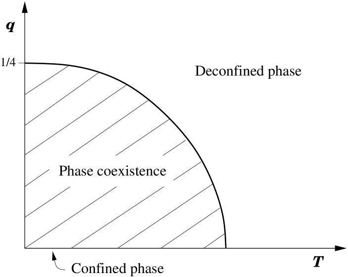
Figure 3: Schematic phase diagram for the free theory in the $q$-$T$ plane. Within the phase coexistence region, the chemical potential is independent of the charge $q$, and equal to its value $\mu_{c}(T)$ on the confinement/deconfinement transition line. Inside the deconfined phase, the chemical potential (at fixed $T$) increases with increasing $q$. Only the $T<T_{c}$ segment of the $q=0$ axis corresponds to the pure deconfined phase. The maximal charge $q_{c}^{\rm max}=1/4$, and the maximum transition temperature $T_{c}^{\rm max}\approx 0.38/R$.

Although the authors of Ref. [22] did not explicitly evalute the chemical potential produced by their thermpdynamic potential, or notice its independence on $q$ for their “small $q$” extremum, the results of Ref. [22] are completely consistent with the above description of phase coexistence in the $q$-$T$ phase diagram.

3 Weak Coupling, High Temperature Effective Theory

We now consider the theory in the high temperature regime, $T\gg 1/R$, with a small non-zero coupling. The relevant expansion parameter will be $1/(TR)^{2}$, so the high temperature regime may also be viewed as the regime of large spatial radius at a fixed temperature. Consequently, for observables which are primarily sensitive to the scale $T$, the curvature of the $S^{3}$ will produce only small corrections to flat space results.

Let $\lambda\equiv g^{2}N_{c}$ denote the usual ’t Hooft coupling, which is held fixed as $N_{c}\to\infty$. Interesting phenomena in the phase diagram will be found to occur when $1/(TR)^{2}$ and $\mu^{2}/T^{2}$ are both of order $\lambda$, so we will focus on this region of parameter space.

At non-zero temperature, one may always decompose fields into Fourier series running over all Matsubara frequencies, and thereby view every four-dimensional field as an infinite tower of three dimensional fields. At high temperature, where the $1/T$ circumference of the periodic time circle is small compared to all other scales, the non-zero Matsubara frequency modes behave (with respect to physics on length scales large compared to $1/T$) like fields describing very heavy excitations with $\mathcal{O}(T)$ mass. As $T\to\infty$, the non-static heavy modes decouple [27] and one may integrate them out leaving only the light zero frequency modes. In this way, one obtains a three dimensional effective theory of the static modes [28]. Convenient techniques for systematically constructing this effective theory, using dimensional continuation to regulate both long and short distance behavior, were described by Braaten and Nieto [29, 30].

There are three scales which are relevant for equilibrium thermodynamics in weakly coupled high temperature non-Abelian gauge theories at zero chemical potential: the temperature $T$​, the “electric mass” (or inverse Debye screening length) which is $\mathcal{O}(\!\sqrt{\lambda}T)$, and the “magnetic mass” (or inverse correlation length of the static gauge field) which is $\mathcal{O}(\lambda T)$. One may construct a dimensionally reduced “electric” effective theory, valid on length scales large compared to $1/T$, by integrating out non-static fluctuations. One may then construct a further reduced “magnetic” effective theory, valid on length scales large compared to $(\sqrt{\lambda}\,T)^{-1}$, by also integrating out static fluctuations on the Debye screening scale. For QCD, these two effective theories are commonly referred to as EQCD₃ and MQCD₃, respectively [30].

For our case of $\mathcal{N}\,{=}\,4$ super-Yang-Mills theory with non-zero chemical potentials, it is the “electric” effective theory which will be of interest. This effective theory, which we will call “ESYM₃”, will contain a three dimensional gauge field $\bf A$, the static component of $A_{0}$, which will appear as an adjoint scalar field, and the static components of the original scalars $\Phi_{A}$. The fermions, having no zero-frequency components due to their antiperiodicity, will be completely integrated out. Operationally, one builds the effective theory by considering all local operators which may be constructed from these fields and are consistent with the symmetries of the theory. Up to any given order in perturbation theory, only a finite number of operators with sufficiently low dimensions are needed. The required coefficients are determined by matching the results for a minimal set of observables which may be evaluated in both the effective and underlying theories [29, 30].

The operators in ESYM₃ include the identity operator, the usual gauge invariant derivative terms, quadratic mass terms for scalar fields, and scalar interaction terms. It is convenient to use rescaled fields in the effective theory,

$$A_{i}\equiv\sqrt{Z_{1}T}\,\tilde{A}_{i}\,,\qquad A_{0}\equiv\sqrt{Z_{2}T}\,\tilde{A}_{0}\,,\qquad\Phi_{A}\equiv\sqrt{Z_{3}T}\>\tilde{\Phi}_{A}\,,$$ (37)

with $Z_{1}$, $Z_{2}$, and $Z_{3}$ dimensionless wavefunction renormalization factors, and $\tilde{A}_{\mu}$ and $\tilde{\Phi}_{A}$ now having canonical dimension 1/2. The wavefunction renormalization factors may be chosen so that the Lagrangian density of the effective theory has the form

$${\cal L}_{{\rm ESYM}_{3}}=f+\,\operatorname{tr}\!\left[{\textstyle\frac{1}{2}}(\tilde{F}_{ij})^{2}+(D_{i}\tilde{A}_{0})^{2}+M_{D}^{2}\,\tilde{A}_{0}^{2}+(D_{i}\tilde{\Phi}_{A})^{2}+m_{A}^{2}\,\tilde{\Phi}_{A}^{2}\right]+{V}(\tilde{A}_{0},\tilde{\Phi}_{A})\,,\vphantom{\Bigg{|}}$$ (38)

where $D_{i}\equiv\partial_{i}+ig_{3}[\tilde{A}_{i},\cdot]$ and $\tilde{F}_{ij}=[D_{i},D_{j}]$, with $g_{3}\equiv g\sqrt{T}$ the dimensionful gauge coupling appropriate for a three-dimensional theory.

The coefficient of the identity operator, $f$, is the 3-$d$ effective theory version of a cosmological constant, and represents the contribution to the free energy density from modes which have been integrated out. Because we are working at high temperature (or large volume) and only integrating out heavy modes with short $\mathcal{O}(1/T)$ correlation lengths, the computation of the free energy density due to heavy modes may be performed entirely in flat space, treating the curvature and chemical potential induced scalar mass terms as small perturbations. Corrections to this approximation will vanish exponentially fast in $TR$ (or faster than any power of $\lambda$, since we are assuming that $TR$ is of order $1/\sqrt{\lambda}$). Details of the calculation are described in appendix B.1. The result, through order $\lambda$, is

$$f=-\frac{N_{c}^{2}\,T^{3}}{12}\bigg{\{}2\pi^{2}-3\lambda-\frac{3}{T^{2}R^{2}}+\sum_{p=1}^{3}\>\frac{2\mu_{p}^{2}}{T^{2}}+\sum_{i=1}^{4}\>\frac{\tilde{\mu}_{i}^{2}}{T^{2}}+\mathcal{O}(\lambda^{2})\bigg{\}}\,.$$ (39)

The mass parameters $m_{A}^{2}$ of the scalar fields $\tilde{\Phi}_{A}$ receive tree-level contributions from the curvature coupling and the chemical potentials, plus $\mathcal{O}(\sqrt{\lambda}\,T)$ one-loop thermal corrections, so that

$$m_{A}^{2}=R^{-2}-\mu_{A}^{2}+\delta m^{2}(T)\,,$$ (40)

where we introduce (for later convenience)

$$\mu_{A}\equiv\begin{cases}\mu_{1}\,,&A=1\mbox{ or }2;\cr\mu_{2}\,,&A=3\mbox{ or }4;\cr\mu_{3}\,,&A=5\mbox{ or }6.\end{cases}$$ (41)

Because we will be interested in the regime where the tree-level contributions nearly cancel, including the thermal mass correction $\delta m^{2}(T)$ is essential. This contribution, as well as the one-loop scalar wavefunction renormalization (which will also be needed) may be obtained by matching the two-point scalar correlator in the original theory at zero frequency and low spatial momentum with the corresponding correlator in the effective theory. The computation is shown in Appendix B.2. The result for the thermal mass (also derived in Refs. [31, 32, 33]) is

$$\delta m^{2}(T)=T^{2}\left[\,\lambda+\mathcal{O}(\lambda^{2})\right].$$ (42)

One-loop fluctuations on the scale $T$ also produce an $\mathcal{O}(\sqrt{\lambda}\,T)$ mass for $\tilde{A}_{0}$. The resulting Debye mass parameter is [31]

$$M_{D}^{2}=T^{2}\left[\,2\lambda+\mathcal{O}(\lambda^{2})\right].$$ (43)

The interaction potential $V(\tilde{A}_{0},\tilde{\Phi}_{A})$ contains both tree-level and fluctuation induced thermal contributions,

$$V(\tilde{A}_{0},\tilde{\Phi}_{A})=V_{\rm tree}(\tilde{A}_{0},\tilde{\Phi}_{A})+\delta V(\tilde{A}_{0},\tilde{\Phi}_{A})\,.$$ (44)

The tree-level part equals the scalar interaction terms of the original four-dimensional action, re-expressed in terms of the rescaled fields (37) (with the wavefunction renormalization factors equal to one at lowest order),

$$V_{\rm tree}(\tilde{A}_{0},\tilde{\Phi}_{A})=\operatorname{tr}\left\{2g_{3}\,\mu_{p}\,([\tilde{A}_{0},\tilde{X}_{p}]\,\tilde{Y}_{p})+g_{3}^{2}\,(i[\tilde{A}_{0},\tilde{\Phi}_{A}])^{2}+{\textstyle\frac{1}{2}}g_{3}^{2}\,(i[\tilde{\Phi}_{A},\tilde{\Phi}_{B}])^{2}\right\}\,.$$ (45)

It is straightforward to obtain one-loop contributions to $\delta V$ that are quartic in $\Phi_{A}$. The coefficient of the quartic term can be computed by evaluating the one-loop heavy-mode contribution to the four-point correlator of the scalar fields with vanishing external momenta. Once again, because we are interested in effects due to heavy modes with correlation lengths small compared to $R$, these contributions may be evaluated in flat space, ignoring both curvature and chemical potential corrections. The required calculation is performed in appendix B.3, with the result

$$\delta V_{\rm quartic}(\tilde{\Phi}_{A})=\frac{\ln 2}{2\pi^{2}}\>\frac{g_{3}^{4}}{T}\,\operatorname{tr}(\tilde{\Phi}^{\rm adj}_{B}\,\tilde{\Phi}^{\rm adj}_{C}\,\tilde{\Phi}^{\rm adj}_{B}\,\tilde{\Phi}^{\rm adj}_{C})\,,$$ (46)

where the trace is in the adjoint representation, with $(\tilde{\Phi}^{\rm adj}_{A})_{ac}\equiv i\tilde{\Phi}_{A}^{b}f^{abc}$. Note that no terms cubic in $\tilde{\Phi}_{A}$ can be generated, since they would not respect the $U(1)^{3}$ subgroup of the $SU(4)$ $R$-symmetry, which is preserved even in the presence of chemical potentials.

One may, in principle, continue in a similar manner and obtain the coefficients of arbitrarily higher dimensional operators in the effective action. However, in the special case where the scalar fields take values in flat directions (which minimize the tree potential), one may employ a more elegant background field method. This method not only confirms the coefficients of the results (42) and (46), it also yields all higher order terms, in powers of $\Phi$, in the one-loop contribution to $\delta V(\Phi_{A})$. This is discussed in Appendix C and the result is

$$\delta V_{\text{flat}}(\tilde{\Phi}_{A}) ={\textstyle\frac{1}{2}}\pi^{2}\>T^{3}\,\operatorname{tr}\!\bigg{[}\,(\ln 2)\Big{(}\frac{g_{3}^{2}}{\pi^{2}T^{2}}\sum_{A}\tilde{\Phi}_{A}^{\text{adj}}\tilde{\Phi}_{A}^{\text{adj}}\Big{)}^{2}$$

$$+\sum_{l=3}^{\infty}\>{8}(1-4^{-l+2})\,\frac{(2l{-}5)!!}{(2l)!!}\,\zeta(2l{-}3)\Big{(}-\frac{g_{3}^{2}}{\pi^{2}T^{2}}\sum_{A}\tilde{\Phi}_{A}^{\text{adj}}\tilde{\Phi}_{A}^{\text{adj}}\Big{)}^{l}\,\bigg{]}\;.$$ (47)

These adjoint representation traces may be written more explicitly in terms of the eigenvalues $\{\tilde{\lambda}_{A}^{m}\}$ of $\tilde{\Phi}_{A}$ (viewed as an $N_{c}\times N_{c}$ matrix). It will prove convenient to introduce dimensionless rescaled eigenvalues,

$$\rho_{A}^{m}\equiv\frac{g_{3}}{\pi T}\>\tilde{\lambda}_{A}^{m}\,,$$ (48)

in terms of which

$$\operatorname{tr}\biggl{[}\Big{(}\frac{g_{3}^{2}}{\pi^{2}T^{2}}\sum_{A}\tilde{\Phi}_{A}^{\text{adj}}\,\tilde{\Phi}_{A}^{\text{adj}}\Big{)}^{l}\,\biggr{]}=\sum_{m,n}\sum_{A}\>(\rho_{A}^{m}-\rho_{A}^{n})^{2l}\,.$$ (49)

Note that when the rescaled eigenvalues $\{\rho_{A}^{m}\}$ (and their differences) are parametrically of order one, then all terms in the series (47) are comparable in size. The potential (47) will play an essential role in the next section, where its behavior will be examined in more detail.

4 High Temperature Thermodynamics

4.1 Deconfined Plasma Phase

The effective scalar masses $m_{A}^{2}$ [given by Eqs. (40) and (42)] are positive as long as the chemical potentials are sufficiently small,

$$\mu_{A}^{2}<R^{-2}+\lambda\,T^{2}\,.$$ (50)

Assuming this is the case, the trivial configuration of vanishing scalar fields,

$$\tilde{\Phi}_{A}=0\,,\qquad\tilde{A}_{0}=0\,,$$ (51)

is a local minimum of the effective potential. The conditions under which this is the global minimum will be examined in the next subsection. Because of the non-zero Debye mass $M_{D}^{2}$ [given by Eq. (43)], the static mode $\tilde{A}_{0}$ has perturbatively small fluctuations in the weak coupling, high temperature regime. Hence, the Polyakov loop expectation value $\langle\operatorname{tr}U(\vec{x})\rangle=\langle\operatorname{tr}e^{i\beta gA_{0}(\vec{x})}\rangle$ is non-zero. So the trivial configuration (51) describes a deconfined plasma phase in which the center symmetry is spontaneously broken while the $U(1)^{3}$ $R$-symmetry (left invariant by the chemical potentials) is unbroken.

The free energy $F=-T\ln Z_{\text{ESYM}_{3}}$, where $Z_{\text{ESYM}_{3}}$ is the partition function of the three-dimensional effective theory (38). In the deconfined plasma phase the order $\lambda^{0}$ and $\lambda^{1}$ contributions to $\beta F$ arise solely from the heavy modes which were integrated out to produce the effective theory. Hence, these contributions are completely contained in the coefficient of the unit operator, $f$, given in Eq. (39). The next contribution is of order $\lambda^{3/2}$ (not $\lambda^{2}$), and comes from static fluctuations of the scalar fields $\tilde{\Phi}_{A}$ and $\tilde{A}_{0}$. In the full theory, evaluation of the order $\lambda^{3/2}$ contribution requires an infinite resummation of ring diagrams. But this becomes an easy one-loop calculation using the high temperature effective theory.

Because the spatial gauge fields $\tilde{A}_{i}$ are massless, their one-loop contribution vanishes (using dimensional continuation). The effective scalar fields $\tilde{A}_{0}$ and $\tilde{\Phi}_{A}$ each make a one-loop contribution to the free energy density of the form

$${\textstyle\frac{1}{2}}N_{c}^{2}\,T\int\frac{d^{3}p}{(2\pi)^{3}}\>\ln(p^{2}+m^{2})=-N_{c}^{2}\,T\>\frac{m^{3}}{12\pi}\,,$$ (52)

where the integral is evaluated using dimensional continuation, and $m$ is the appropriate mass parameter for the field. So the entire $\mathcal{O}(\lambda^{3/2})$ contribution to the free energy density is

$$-\frac{N_{c}^{2}\,T}{12\pi}\Bigl{(}M_{D}^{3}+\sum_{A=1}^{6}m_{A}^{3}\Bigr{)}\,.$$ (53)

Inserting the explicit expressions (40)–(43) for these masses, and adding ($T$ times) the coefficient $f$ of the unit operator (39), we obtain the free energy in the deconfined plasma phase, through order $\lambda^{3/2}$,

$$F_{\rm plasma}=-\frac{N_{c}^{2}}{12}\>T^{4}\,\mathcal{V}\,\bigg{\{}2\pi^{2} -3\lambda-\frac{3}{T^{2}R^{2}}+\sum_{p=1}^{3}\frac{2\mu_{p}^{2}}{T^{2}}+\sum_{i=1}^{4}\frac{\tilde{\mu}_{i}^{2}}{T^{2}}$$

$$+\frac{(2\lambda)^{3/2}}{\pi}+\frac{2}{\pi}\sum_{p=1}^{3}\left(\lambda+\frac{1}{T^{2}R^{2}}-\frac{\mu_{p}^{2}}{T^{2}}\right)^{3/2}+\mathcal{O}(\lambda^{2})\bigg{\}}\;,$$ (54a)

with $\mathcal{V}\equiv 2\pi^{2}R^{3}$ the spatial volume. Note that this expression is only valid (and real) when the chemical potentials satisfy the inequality (50).

4.2 Is There a Higgs Phase?

Now consider the situation when the maximal chemical potential exceeds $\lambda T^{2}+R^{-2}$, so that some of the effective scalar masses $m_{A}^{2}=\lambda T^{2}+R^{-2}-\mu_{A}^{2}$ become negative. This makes the quadratic terms in the ESYM₃ scalar potential unstable, so the minimum of the effective theory scalar potential can no longer lie at the origin. However, one may verify that the sum of the tree (45) and one-loop (46) quartic contributions to the scalar potential is positive definite for all non-zero $\tilde{\Phi}_{A}$, showing that the quartic thermal corrections to the effective potential lift the flat directions which are present in the tree-level potential.

This suggests that thermal corrections to the scalar interactions in the effective theory may stabilize the theory when chemical potentials are large, generating a non-trivial minimum of the effective scalar potential. Such a non-trivial minimum would correspond to a Higgs phase with spontaneously broken $R$-symmetry.

Assume (for the moment) that terms in the scalar potential involving higher than quartic powers of the field are unimportant. One can explicitly minimize the quadratic plus quartic contributions to the ESYM₃ scalar potential. At the minimum one is balancing an unstable tree-level quadratic term against a one-loop quartic term, so the rescaled eigenvalues (48) of the scalar fields $\tilde{\Phi}_{A}$ are of order

$$(\rho_{A}^{m})^{2}\sim\frac{|m_{A}^{2}|}{\lambda T^{2}}\,.$$ (55)

The corresponding value of the (truncated) potential, at its minimum, scales as

$$-N_{c}^{2}\,T^{3}\left[\max_{A}\Bigl{(}-\frac{m_{A}^{2}}{\lambda T^{2}}\Bigr{)}\right]^{2}.$$ (56)

However, minimizing the truncated scalar potential and adding its value to the coefficient of the identity operator (39) does not produce a valid approximation for the free energy and, as we will see, this putative Higgs phase simply does not exist.

There are two problems with the above scenario suggesting the presence of a Higgs phase. First, we neglected higher than quartic terms in the ESYM₃ potential (47). This is only acceptable if $(\rho_{A}^{m})^{2}\ll 1$ which, given the above estimate, requires $|m_{A}^{2}|\ll\lambda T^{2}$. The curvature and chemical potential contributions to $m_{A}^{2}$ are, by previous assumption, individually of order $\lambda T^{2}$. So neglecting terms higher than quartic in the potential requires that $m_{A}^{2}$ be parametrically smaller than its individual pieces. In other words, one must restrict attention to a “fine-tuned” region in the phase diagram sufficiently close to the surface where an effective scalar mass first turns negative.

Second, and more importantly, the above scenario was based on a classical analysis of the action (38) of the effective theory — so it neglected the effects of fluctuations in the static ESYM₃ fields. To see if this matters, let

$$\tilde{\Phi}_{A}=\langle\tilde{\Phi}_{A}\rangle+\delta\tilde{\Phi}_{A}\,,$$ (57)

with the mean value $\langle\tilde{\Phi}_{A}\rangle$ lying along a flat direction of the tree-level potential. That implies that the mean values are simultaneously diagonal, $\langle(\tilde{\Phi}_{A})_{mn}\rangle=(\pi T/g_{3})\,\rho_{A}^{m}\,\delta_{mn}$ (up to an irrelevant gauge transformation). Inserting the decomposition (57) into the tree-level potential (45) leads to non-zero mass corrections for the off-diagonal components of the scalar field and $\tilde{A}_{0}$ fluctuations,

$$\delta V_{\rm tree}(\tilde{\Phi}_{A})=\sum_{m,n}\>M_{mn}^{2}\,\Bigl{\{}\bigl{|}(\tilde{A}_{0})_{mn}\bigr{|}^{2}+\sum_{B}\bigl{|}(\delta\tilde{\Phi}_{B})_{mn}\bigr{|}^{2}\Bigr{\}}+\mathcal{O}(\delta\tilde{\Phi}^{3})+\mathcal{O}(\delta\tilde{\Phi}\tilde{A}_{0}^{2})\,,$$ (58)

with

$$M_{mn}^{2}\equiv\pi^{2}T^{2}\,\sum_{A}(\rho_{A}^{m}-\rho_{A}^{n})^{2}\,.$$ (59)

And inserting (57) into the scalar kinetic term produces mass terms for the off-diagonal components of the static gauge field, $\operatorname{tr}(D_{i}\tilde{\Phi}_{A})^{2}=\sum_{m,n}\>M_{mn}^{2}\,\bigl{|}(\tilde{A}_{i})_{mn}\bigr{|}^{2}+\cdots\,.$

If the (rescaled) diagonal components $\{\rho_{A}^{m}\}$ are $\mathcal{O}(1)$, then the mass terms (59) for off-diagonal fields induced by the mean values of the diagonal components will be of order $T^{2}$, or large compared to the $\mathcal{O}(\lambda T^{2})$ thermal contributions due to the non-zero frequency modes, as well as the curvature and chemical potential induced mass terms [which we have assumed to also be $\mathcal{O}(\lambda T^{2})$]. It will be sufficient to focus on this regime; if a Higgs phase does exist, then the typical size of $\rho_{A}^{m}$ will need to be of this order. Consequently, if the scalar fields $\tilde{\Phi}_{A}$ have non-trivial mean values lying along flat directions of the tree-level potential, then off-diagonal components of the static fields will act like heavy degrees of freedom (just like the non-static Matsubara modes) and need to be integrated out before considering the dynamics of the remaining “light” diagonal modes.

Doing so is straightforward; the basic ingredient is just the three dimensional loop integral (52). The result is a “Higgs-branch” three-dimensional effective theory which we will term “HSYM₃” and whose Lagrange density has the form

$${\cal L}_{{\rm HSYM}_{3}}=\,\operatorname{tr}\!\left[{\textstyle\frac{1}{2}}(\tilde{F}_{ij})^{2}+(D_{i}\tilde{A}_{0})^{2}+M_{D}^{2}\,\tilde{A}_{0}^{2}+(D_{i}\tilde{\Phi}_{A})^{2}\right]+\overline{V}(\tilde{\Phi}_{A})\,,$$ (60)

where the fields are now diagonal, with gauge group $[U(1)]^{N_{c}-1}$. The scalar potential $\overline{V}(\tilde{\Phi}_{A})$ for the remaining diagonal components is

$$\overline{V}(\tilde{\Phi}_{A}) =f+\operatorname{tr}(m_{A}^{2}\,\tilde{\Phi}_{A}^{2})+\delta V_{\rm flat}(\tilde{\Phi}_{A})+\delta V_{\rm off-diag}(\tilde{\Phi}_{A})\,,$$ (61)

where $f$ is the additive constant (39) due to the non-zero frequency modes, $\delta V_{\rm flat}(\tilde{\Phi}_{A})$ is the one-loop potential (47) induced by non-zero frequency fluctuations, and

$$\delta V_{\rm off-diag}(\tilde{\Phi}_{A})=-{\textstyle\frac{2}{3}}\pi^{2}\>T^{3}\,\operatorname{tr}\!\bigg{[}\Big{(}\frac{g_{3}^{2}}{\pi^{2}T^{2}}\sum_{A}\tilde{\Phi}_{A}^{\text{adj}}\tilde{\Phi}_{A}^{\text{adj}}\Big{)}^{3/2}\bigg{]}.$$ (62)

Writing this explicitly in terms of the rescaled eigenvalues $\{\rho_{A}^{m}\}$ of $\tilde{\Phi}_{A}$, the potential is

$$\overline{V}(\rho_{A}^{m})={\textstyle\frac{1}{2}}\pi^{2}\,T^{3}\sum_{m,n}\bigg{[}\,h(\rho^{mn})+\sum_{A}\delta\hat{m}_{A}^{2}\,(\rho_{A}^{m}{-}\rho_{A}^{n})^{2}\bigg{]}\,,$$ (63)

where we have defined an rms measure of eigenvalue differences,

$$\rho^{mn}\equiv\Big{[}\sum_{A}\big{(}\rho_{A}^{m}-\rho_{A}^{n}\big{)}^{2}\Big{]}^{1/2}\,,$$ (64)

introduced the rescaled mass shift

$$\delta\hat{m}_{A}^{2}\equiv\frac{m_{A}^{2}}{\lambda T^{2}}-1=\frac{R^{-2}-\mu_{A}^{2}}{\lambda T^{2}}\;,$$ (65)

and defined the one-dimensional function

$$h(v)=-{\textstyle\frac{1}{3}}+v^{2}-{\textstyle\frac{4}{3}}\,v^{3}+(\ln 2)\,v^{4}+\sum_{l=3}^{\infty}8\,(1-4^{-l+2})\,\frac{(2l{-}5)!!}{(2l)!!}\,\zeta(2l{-}3)\,(-v^{2})^{l}\,.$$ (66)

The additive constant $-\frac{1}{3}$ comes from $f$. We have dropped subleading $\mathcal{O}(\lambda T^{3})$ contributions to $f$, as these are parametrically smaller than the $\mathcal{O}(T^{3})$ terms retained in $\overline{V}$.

Inserting the defining series for the zeta function and interchanging summations allows one to re-express $h(v)$ in an alternative form which is more convenient for examining its global behavior, namely

$$h(v)=-{\textstyle\frac{1}{3}}+v^{2}-{\textstyle\frac{4}{3}}\,v^{3}+{\textstyle\frac{8}{3}}\sum_{j=1}^{\infty}\>(-1)^{j-1}\left[(j^{2}{+}v^{2})^{3/2}-j^{3}-{\textstyle\frac{3}{2}}v^{2}\,j\right]\,.$$ (67)

The function $h(v)$ is graphed in Figure 4. For large arguments, $h(v)$ approaches zero exponentially rapidly,

$$h(v)\sim-\frac{4}{\pi^{2}}\,(2v)^{3/2}\,e^{-\pi v}\,.$$ (68)

The approach to zero as $v\to\infty$ may be understood as a consequence of supersymmetry. In the potential (63), the argument $\rho^{mn}$ of the function $h$ is the ratio of the mass scale $M_{mn}$ for the off-diagonal fields to ($\pi$ times) the temperature. A large ratio is equivalent to sending $T\rightarrow 0$ while holding this mass scale fixed. (Since we are assuming $1/(TR)^{2}\sim\mu^{2}/T^{2}\sim\lambda$, this also implies sending $R\rightarrow\infty$ and $\mu\to 0$.) At zero temperature, supersymmetry requires that all loop contributions to the effective potential cancel. So the cancellation of contributions to the one-loop potential as eigenvalue differences become large follows from the cancellation of one-loop contributions as $T\to 0$.

Figure 4: Graph of the function $h(v)$, defined in Eq. (67).

Figure 5: Plots of the scalar potential $\overline{V}$, divided by the overall factor $c\equiv{\textstyle\frac{1}{2}}\pi^{2}N_{c}^{2}T^{3}$, for the eigenvalue configuration $\rho_{A}^{m}=v\,\delta_{A}^{1}\,(-1)^{m}$, as a function of $v$. The four plots correspond to $\delta\hat{m_{A}}^{2}=0.2$, $0.0$, $-0.05$ and $-1$, respectively. Note that half of the eigenvalues differences $\rho^{mn}$ are zero in this configuration, and each vanishing difference contributes $h(0)=-\frac{1}{3}$ to $\overline{V}/({\textstyle\frac{1}{2}}\pi^{2}T^{3})$. This accounts for the non-zero asymptotic value in case (b). If $\delta\hat{m}_{A}^{2}$ is positive (or zero), then the potential is monotonically increasing with a unique minimum at the origin. If $-1<\delta\hat{m}_{A}^{2}<0$, then the potential is unbounded below, with a local minimum at the origin. If $\delta\hat{m}_{A}^{2}<-1$, then the potential is monotonically decreasing with a maximum at the origin.

As indicated in Eq. (63), the complete potential $\overline{V}(\rho_{A}^{m})$ is a sum of values of $h(v)$ plus the sum of squares of the eigenvalue differences weighted by the mass shift $\delta\hat{m}_{A}^{2}$. Plots of the resulting potential, for a simple eigenvalue distribution and several choices of mass shifts, are shown in Figure 5. Since the function $h(v)$ is bounded (for positive real $v$), it is evident that the potential $\overline{V}(\rho_{A}^{m})$ will be unbounded below if any mass shift $\delta\hat{m}_{A}^{2}$ is negative. Since $\delta\hat{m}_{A}^{2}\propto R^{-2}-\mu_{A}^{2}$, this means that no truly stable equilibrium phase can exist if any chemical potential exceeds $1/R$. Moreover, the potential $\overline{V}(\rho_{A}^{m})$ has no local minimum for any non-zero set of eigenvalues $\{\rho_{A}^{m}\}$. Hence there is no Higgs phase (not even a metastable Higgs phase) in this weakly coupled, high temperature theory.

4.3 High Density Metastability

When the largest chemical potential lies in the interval

$$R^{-2}<\mu^{2}<\lambda T^{2}+R^{-2}\,,$$ (69)

the deconfined plasma phase (corresponding to the origin of the field space) is locally stable, but is not the global minimum of the free energy — as there is no global minimum. For this range of chemical potential and finite $N_{c}$, as we will see, the deconfined plasma is metastable with a lifetime which grows exponentially as $N_{c}\to\infty$. The onset of instability, at a (maximal) chemical potential of $1/R$, is independent of $\lambda$ and thus exactly where the free theory becomes ill-defined. This may be understood as a consequence of the existence of towers of BPS operators with vanishing anomalous dimensions (independent of $\lambda$) which map to towers of BPS states on $S^{3}$ with energies precisely equal to their $R$-charge. Consequently, the Boltzmann sum representation of the partition function ceases to converge if any chemical potential exceeds $1/R$. However, this does not prevent the existence of an arbitrarily long-lived metastable phase above this threshold.

To estimate the decay rate when $\mu>1/R$, consider the behavior of the effective potential $\overline{V}(\tilde{\Phi}_{A})$ for configurations of the form

$$\rho_{A}^{m}=v\,\delta_{A,1}\,(\delta_{m,1}-1/N_{c})\,,$$ (70)

for some dimensionless real number $v$. All but one of the eigenvalues remain near the origin in this configuration as the single eigenvalue $\rho_{1}^{1}\equiv v\,(1{-}\frac{1}{N_{c}})$ is varied. (This configuration satisfies the $SU(N_{c})$ tracelessness constraint, $\sum_{m}\rho_{A}^{m}=0$.) Assume that $\mu_{1}$ is the largest chemical potential. For this class of configurations, the potential $\overline{V}(\tilde{\Phi}_{A})$ becomes

$$\overline{V}(v)=-{\textstyle\frac{1}{6}}\pi^{2}T^{3}N_{c}^{2}+\pi^{2}T^{3}N_{c}\,[\,h(v)+{\textstyle\frac{1}{3}}+\delta\hat{m}_{1}^{2}\,v^{2}]+\mathcal{O}(N_{c}^{0})\,.$$ (71)

The interval (69) corresponds to $\delta\hat{m}_{1}^{2}\equiv(R^{-2}-\mu_{1}^{2})/(\lambda T^{2})$ lying between 0 and $-1$. A plot of $\overline{V}(v)$ resembles case (c) of Fig. 5, with a potential barrier separating the region near $v=0$ from the bottomless region at large values of $v$. However, for the eigenvalue configuration (70) the height of this potential barrier grows only linearly with $N_{c}$,

$$\Delta\overline{V}\equiv\max_{v}\overline{V}(v)-\overline{V}(0)=\mathcal{O}(N_{c}\,T^{3})\,.$$ (72)

As seen from Eq. (63), this potential difference receives contributions from every pair of unequal eigenvalues of $\tilde{\Phi}_{1}$ and, for this configuration, only $2(N_{c}{-}1)$ terms involving the difference between $\rho_{1}^{1}$ and the other $N_{c}{-}1$ eigenvalues of $\tilde{\Phi}_{1}$ contribute.

The deconfined plasma phase corresponding to $v=0$ can decay via a thermal fluctuation in which a single eigenvalue makes a large excursion from the origin to top of the barrier, uniformly in space. The probability for such a fluctuation has a Boltzmann suppression factor of

$$e^{-\mathcal{V}\,\Delta\overline{V}}=e^{-\mathcal{O}(N_{c}\,(TR)^{3})}\,,$$ (73)

where $\mathcal{V}=2\pi^{2}R^{3}$ is the spatial volume. (The usual factor of $\beta=1/T$ appearing in a Boltzmann factor was absorbed in our definition of the scalar potential of the three dimensional effective theory.)

Alternatively, a thermal fluctuation could nucleate a critical bubble in which a single eigenvalue makes a large excursion to values across the barrier with lower free energy density, over a sufficiently large spatial region so that bubble subsequently grows. The process is characterized by a Euclidean bounce solution [35, 36]. The required size of the critical bubble scales as $(\sqrt{\lambda}T)^{-1}$. The action (in the effective theory) for such a solution is $\mathcal{O}(N_{c}/\lambda^{3/2})$, so the rate for this process will have a Boltzmann suppression factor of

$$e^{-S_{\rm bounce}}=e^{-\mathcal{O}(N_{c}\,\lambda^{-3/2})}\,.$$ (74)

When $1/(TR)=\mathcal{O}(\sqrt{\lambda})$, which we have assumed, then both processes will have rates which are exponentially suppressed by an amount which scales as $N_{c}/\lambda^{3/2}$. Which process dominates depends on the pure numerical coefficients in the exponents of (73) and (74) [which we have not evaluated] together with the value of $\sqrt{\lambda}\,TR$. Consequently, despite the fact that no true equilibrium state exists when $\mu>1/R$, as long as the maximal chemical potential is within the interval (69), the deconfined plasma phase will be metastable with a lifetime which diverges exponentially as $N_{c}\to\infty$.

The region of deconfined plasma metastability terminates when the largest chemical potential reaches a maximal value,

$$\mu_{\rm max}(T)=\sqrt{\lambda T^{2}+R^{-2}}\times[1+\mathcal{O}(\lambda)]\,,$$ (75)

at which point the effective thermal mass of one or more of the scalar fields becomes negative. This is analogous to “spinodal decomposition,” which determines the limit of supercooling or superheating at a typical first order phase transition. However, for weakly coupled $\mathcal{N}\,{=}\,4$ SYM, no new equilibrium state exists for $\mu>\mu_{\rm max}$.

5 Summary and Comparison with Dual Gravitational Analysis

Figure 6: The phase structure of the weakly coupled gauge theory on the left, and of gravitational solutions to 5-$d$ supergravity, believed to correspond to the strongly coupled gauge theory, on the right. For both figures, $\mu$ is the largest of the three chemical potentials. In the weak coupling diagram, the location of the phase boundary forming the upper limit of the metastable plasma phase has not been evaluated at low temperature; this portion of the boundary is indicated by the dashed line. In the strong coupling diagram, $T_{0}$ is the temperature at which the black hole radius reaches to zero. Its value depends on the pattern of chemical potentials and equals $(\pi R)^{-1}$ for a single non-zero charge, while $T_{0}=0$ for three equal charges.

The resulting phase diagram for weakly coupled $\mathcal{N}\,{=}\,4$ supersymmetric Yang-Mills theory is sketched on the left side of Figure 6. A confinement/deconfinement transition line separates a confining phase at lower temperature or chemical potential from a deconfined plasma phase at higher temperature or chemical potential. The location of this line is known in the $\lambda\to 0$ limit but, for the reasons discussed in section 2, the order of this phase transition (at small but non-zero coupling) is not currently known. If the maximal chemical potential exceeds $1/R$, then no truly stable equilibrium state exists. But, at least for sufficiently high temperatures ($T\gg 1/R$), the deconfined plasma remains metastable beyond $\mu=1/R$, with a lifetime which grows exponentially as $N_{c}\to\infty$. This metastable region terminates at a spinodal decomposition phase boundary when the largest chemical potential reaches a limiting value $\mu_{\rm max}(T)$. The $\mu=\mu_{\rm max}(T)$ boundary line asymptotically rises linearly with temperature with slope $\sqrt{\lambda}$, regardless of how many chemical potentials reach $\mu_{c}(T)$ simultaneously.

When $T\lesssim 1/R$, the location of the spinodal decomposition phase boundary is not currently known (at non-zero but weak coupling). Neither are order $\lambda$ corrections to the location of the confinement/deconfinement transition line. It is possible that the phase boundary remains separated from the confinement/deconfinement transition line for all non-zero temperatures, with both lines intersecting at $T=0$ and $\mu=1/R$. This possibility is sketched in Fig. 6. But, for non-zero couplings, the confinement/deconfinement transition line may instead intersect the phase boundary line at a non-zero temperature. In other words, the deconfined plasma region of the phase diagram could pinch off before reaching zero temperature. In this case, for sufficiently low temperature, the confined phase might extend all the way to the boundary of the phase diagram at $\mu=\mu_{\rm max}(T)$, with no intervening phase transitions. Which possibility occurs may well depend on the particular pattern of chemical potentials (for example, whether two or more chemical potentials coincide).

The right side of Fig. 6 shows a sketch of the behavior of gravitational solutions of five dimensional $\mathcal{N}=2$ gauged supergravity, which are believed to be related to the strong coupling limit of $\mathcal{N}\,{=}\,4$ supersymmetric Yang-Mills [17, 18]. The similarities are obvious (in contrast to the previous situation depicted in Fig. 1). A qualitatively similar confinement/deconfinement (or Hawking-Page) transition line is present on both sides. For the black hole, this transition is known to be first order. The black hole instability line, where small perturbations become thermodynamically unstable, appears completely analogous to the spinodal decomposition phase boundary of the weak coupling diagram. The black hole instability line rises linearly for temperatures large compared to the inverse of the AdS₅ curvature radius, $1/R$, but the slope depends on the pattern of chemical potentials (unlike the case at weak-coupling). With only one non-zero potential, for example, the asymptotic slope is $\pi/\sqrt{2}$, while for three equal chemical potentials the slope is $2\pi$.

As noted in footnote 5 of the Introduction, the temperature $T_{0}$ at which the Hawking-Page transition line meets the black hole instability line depends on the pattern of chemical potentials. For three equal chemical potentials (or equivalently three equal charges), $T_{0}=0$. With a single non-zero charge, the temperature $T_{0}=(\pi R)^{-1}$. In every case, the chemical potential at the intersection of the instability and Hawking-Page transition lines is $1/R$. This intersection corresponds to the point where the black hole horizon radius shrinks to zero. Since the phase diagram in the strong coupling region is obtained by comparing the values of the action for black hole and AdS solutions at the same temperature, the region of the phase diagram below $T_{0}$ is completely undetermined.

Ignoring the low temperature region (where limited knowledge on both sides prevents a clear comparison), there is one glaring difference between the weak and strong coupling phase diagrams of Fig. 6 — the non-perturbative metastability of the deconfined plasma phase when the maximal chemical potential exceeds $1/R$. If there is a smooth interpolation between weak and strong coupling, then there must be a similar non-perturbative black hole instability, with an exponentially suppressed nucleation rate whose exponent scales linearly with $N_{c}$. No such instability, with an onset precisely at $\mu=1/R$, is currently known in the gravity dual.

6 Outlook

There are a variety of possible extensions which should be feasible and which would shed light on some of the issues discussed in this paper.

On the gravitational side, investigation into non-perturbative instabilities of RN-AdS black holes (and their generalizations to $\mathcal{N}=8$ gauged supergravity) is clearly needed. Our weak coupling results, plus presumed smooth interpolation between weak and strong coupling, requires the existence of a non-perturbative black hole instability with an onset (at $\mu=1/R$) prior to the known point of perturbative instability.

Under gauge/string duality, the eigenvalues of $\mathcal{N}=4$ SYM scalar fields are identified with the locations of D3-branes in Type IIB string theory. The $R$-charged black hole solutions arise from spinning D3-branes [18]. This suggests that the string theory manifestation of the non-perturbative gauge theory instability should involve a stack of D3-branes, for sufficiently high spin, splitting up into widely separated branes. For $\mu>1/R$, the force between branes at sufficiently large separation should become repulsive. Since the dominant instability in the gauge theory involves a large excursion of a single eigenvalue, the dominant high-spin D3-brane instability should involve a single brane separating from the rest of the stack. It should be possible to verify this scenario with a probe-brane analysis in the RN-AdS background.

Alternatively, one may consider the analogue of non-perturbative gauge theory instabilities involving large excursions by multiple eigenvalues, namely a process in which a stack of $N_{c}$ coincident D3-branes separates into a multi-stack configuration, with each stack containing an order one fraction of the $N_{c}$ branes. (Fig. 5c and d correspond to the simplest case of a symmetric two-stack instability.) Though subdominant, this decay process should be well described by supergravity approximations.

Finding such an instability for spinning D3-branes, with the expected onset threshold of $\mu=1/R$, would provide further evidence supporting a smooth interpolation between weak and strong coupling in $\mathcal{N}\,{=}\,4$ supersymmetric Yang-Mills theory (and the validity of AdS/CFT duality). It might also clarify the puzzle, mentioned in Section 5, involving the behavior of the gravitational system with large but unequal chemical potentials, at temperatures below $T_{0}$ (where the horizon radius of the $R$-charged black hole shrinks to zero). At the moment, no upper limit on the chemical potential of the gravitational phase diagram in this regime in known.

Turning now to the weak coupling analysis, the order of the confinement/deconfinement phase transition at non-zero coupling remains uncertain, for the reasons discussed in Section 2. Its determination requires a three-loop computation similar to (but more complicated than) the one carried out for large $N_{c}$ pure Yang-Mills theory in Ref. [8]. This computation, if carried out for non-zero chemical potentials, would also allow one to determine how weak coupling corrections shift the location of the transition line, which is of particular interest at low temperature where the transition line approaches the spinodal decomposition line. If the interpolation between weak and strong coupling in $\mathcal{N}\,{=}\,4$ SYM is smooth, then the confinement/deconfinement transition is expected to be first order. Confirming (or refuting) this directly would clearly be desirable.

Finally, our weak coupling analysis focused on the high temperature regime, $T\gg 1/R$. Extending the treatment to $T\lesssim 1/R$ would be valuable. For $T\ll 1/R$ one has a large time circle and a small spatial sphere, so the non-zero angular momentum modes on the three-sphere are heavy and may be integrated out, leading to an effective one dimensional quantum mechanics. Analysis of the resulting effective theory should reveal the behavior of the spinodal decomposition phase boundary in the low temperature region, determine whether it intersects the confinement/deconfinement transition line at a non-zero temperature $T_{0}$, and perhaps even reveal a distinct high density, low temperature phase.

Appendix A Derivation of Matrix Model with Chemical Potentials

To reduce the partition function of the free theory (constrained by Gauss’ law) to the matrix model, as sketched in section 2.3, one first separates the zero mode of $A_{0}$ by replacing

$$A_{\nu}(x)\longrightarrow\tilde{A}_{\nu}(x)+\delta_{\nu,0}\,a/g\;,$$ (76)

where $a$ is a constant traceless Hermitian $N_{c}\times N_{c}$ matrix, and $\tilde{A}_{0}$ is orthogonal to the constant mode. Without loss of generality, we may assume that $a$ is diagonal and we denote its entries (or eigenvalues) by $\{q^{m}\,|\,m=1,\cdots,N_{c}\}$ where the $q^{m}$ are all real and satisfy $\sum_{m}q^{m}=0$. One plugs this shifted form of the gauge field into the Lagrangian (2.2) and then sends $g\to 0$. It is convenient to choose the gauge defined by the gauge-fixing term,

$$\operatorname{tr}\{(\partial_{\nu}\tilde{A}_{\nu}+i\,[a,\tilde{A}_{0}])^{2}\}\;.$$ (77)

Define, for convenience, $q^{mn}\equiv q^{m}-q^{n}$ and $\Box^{mn}\equiv(\partial_{\nu}+iq^{mn}\delta_{\nu,0})^{2}$. The Lagrangian of the free theory may be rewritten as the quadratic form

$$\hat{\mathcal{L}}_{\text{quad}}=\sum_{m,n} \bigg{\{}(\tilde{A}_{\nu})^{*}_{mn}(-\Box^{mn})(\tilde{A}_{\nu})_{mn}$$

$$+((X_{p})^{*}_{mn},(Y_{p})^{*}_{mn})\begin{pmatrix}-\Box^{mn}+1-\mu_{p}^{2}&2i\mu_{p}(\partial_{0}+iq^{mn})\\ -2i\mu_{p}(\partial_{0}+iq^{mn})\;&-\Box^{mn}+1-\mu_{p}^{2}\end{pmatrix}\begin{pmatrix}(X_{p})_{mn}\\ (Y_{p})_{mn}\end{pmatrix}$$

$$+(\bar{\psi}_{i})^{*}_{mn}(i{\partial}\negthickspace{\negthickspace{/}}-\gamma_{0}\,q^{mn}-i\tilde{\mu}_{i}\gamma_{0}\gamma_{5})(\psi_{i})_{mn}\bigg{\}}\;,$$ (78)

where the color indices $m,n$ are now explicit, with $(\tilde{A}_{\nu})_{mn}\equiv\tilde{A}_{\nu}^{a}\,(T^{a})_{mn}$ and likewise for the other fields.

Table 2 in section 2.3 lists the eigenvalues of the spatial small fluctuation operators whose eigenfunctions are (scalar, vector, or spinor) spherical harmonics. Denote these eigenvalues by $\Delta_{g}^{2}$, $\Delta_{s}^{2}$ and $\Delta_{f}^{2}$ for the transverse spatial gauge, conformal scalar, and spinor fields, respectively. Denote the Matsubara frequencies by $\omega_{k}$, for either bosons or fermions (as determined by context). Then the contribution to $\ln Z$ from the gauge bosons and ghosts (equal to $-{\textstyle\frac{1}{2}}$ times the logarithm of their functional determinant) is

$$\ln Z_{\rm g}=-{\textstyle\frac{1}{2}}\biggl{[}\sum_{k}\sum_{m,n}\operatorname{tr}\ln\{(\omega_{k}+q^{mn})^{2}+\Delta_{g}^{2}\}-\operatorname{tr}\ln(\omega_{k}^{2}+\Delta_{g}^{2})\biggr{]}\;.$$ (79)

The trace is over the space of transverse vector fields on $S^{3}$. The contribution from gauge-fixing ghosts cancels the contributions from $\tilde{A}_{0}$ and longitudinal part of the spatial gauge field, thereby effectively leaving two transverse gauge field degrees of freedom. (This factor of two is included in the degeneracy factor for transverse vector fields listed in Table 2.) The second term compensates for the fact that there are really only $N_{c}{-}1$ independent diagonal components of the gauge field, not $N_{c}$, because we are dealing with the gauge group $SU(N_{c})$.

Block-diagonalizing the linear operator in (78) for the scalars (by working in the eigenspaces of $\partial_{0}$ and the spatial Laplacian) and taking the determinant in each block gives the scalar contribution of

$$\ln Z_{\rm s}=-{\textstyle\frac{1}{2}}\sum_{k}\sum_{p}\bigg{[}\sum_{m,n} \operatorname{tr}\ln\Bigl{[}\{(\omega_{k}+q^{mn}+i\mu_{p})^{2}+\Delta_{s}^{2}\}\{(\omega_{k}+q^{mn}-i\mu_{p})^{2}+\Delta_{s}^{2}\}\Bigr{]}$$

$$-{} \operatorname{tr}\ln\Bigl{[}\{(\omega_{k}+i\mu_{p})^{2}+\Delta_{s}^{2}\}\{(\omega_{k}-i\mu_{p})^{2}+\Delta_{s}^{2}\}\Bigr{]}\bigg{]}\;.$$ (80)

Similarly, the fermions give

$$\ln Z_{\rm f}={\textstyle\frac{1}{2}}\sum_{k}\sum_{i}\bigg{[}\sum_{m,n} \operatorname{tr}\ln\Bigl{[}\{(\omega_{k}+q^{mn}+i\tilde{\mu_{i}})^{2}+\Delta_{f}^{2}\}\{(\omega_{k}+q^{mn}-i\tilde{\mu_{i}})^{2}+\Delta_{f}^{2}\}\Bigr{]}$$

$$-{} \operatorname{tr}\ln\Bigl{[}\{(\omega_{k}+i\tilde{\mu}_{i})^{2}+\Delta_{f}^{2}\}\{(\omega_{k}-i\tilde{\mu}_{i})^{2}+\Delta_{f}^{2}\}\Bigr{]}\bigg{]}\;.$$ (81)

In integrating out the fermions, it is essential to recall that $\psi_{i}$ is a Majorana fermion. So $\psi_{i}$ and $\bar{\psi}_{i}$ are not independent and the Grassmann integral gives the Pfaffian of $({\partial}\negthickspace{\negthickspace{/}}+i\gamma_{0}\,q^{mn}-\tilde{\mu}_{i}\gamma_{0}\gamma_{5})$, not the determinant.

The Matsubara frequency sums can be carried out (most easily by differentiating with respect to $\Delta^{2}$, performing the sum, and then integrating back in $\Delta^{2}$) and yield

$$\ln Z_{\rm g} =-{\textstyle\frac{1}{2}}\sum_{m,n}\operatorname{tr}\ln\Bigr{[}\{1-e^{-\beta(\Delta_{g}+iq^{mn})}\}\{1-e^{-\beta(\Delta_{g}-iq^{mn})}\}\Bigl{]}+\operatorname{tr}\ln(1-e^{-\beta\Delta_{g}})\,,$$ (82a)

$$\ln Z_{\rm s} =-\sum_{p}\bigg{[}{\textstyle\frac{1}{2}}\sum_{m,n}\operatorname{tr}\ln\Bigl{[}\{1-e^{-\beta(\Delta_{s}+\mu_{p}+iq^{mn})}\}\{1-e^{-\beta(\Delta_{s}+\mu_{p}-iq^{mn})}\}$$

$$\kern 91.04872pt{}\times\{1-e^{-\beta(\Delta_{s}-\mu_{p}+iq^{mn})}\}\{1-e^{-\beta(\Delta_{s}-\mu_{p}-iq^{mn})}\}\Bigr{]}$$

$$\kern 62.59596pt{}-\operatorname{tr}\ln\Bigl{[}\{1-e^{-\beta(\Delta_{s}+\mu_{p})}\}\{1-e^{-\beta(\Delta_{s}-\mu_{p})}\}\Bigr{]}\bigg{]}\;,$$ (82b)

$$\ln Z_{\rm f} =\sum_{i}\bigg{[}{\textstyle\frac{1}{2}}\sum_{m,n}\operatorname{tr}\ln\Bigl{[}\{1+e^{-\beta(\Delta_{f}+\tilde{\mu_{i}}+iq^{mn})}\}\{1+e^{-\beta(\Delta_{f}+\tilde{\mu_{i}}-iq^{mn})}\}$$

$$\kern 82.51282pt{}\times\{1+e^{-\beta(\Delta_{f}-\tilde{\mu_{i}}+iq^{mn})}\}\{1+e^{-\beta(\Delta_{f}-\tilde{\mu_{i}}-iq^{mn})}\}\Bigr{]}$$

$$\kern 56.9055pt{}-\operatorname{tr}\ln\Bigl{[}\{1+e^{-\beta(\Delta_{f}+\tilde{\mu}_{i})}\}\{1+e^{-\beta(\Delta_{f}-\tilde{\mu}_{i})}\}\Bigr{]}\bigg{]}\;.$$ (82c)

In these expressions, we have dropped temperature independent terms that do not contribute to the thermodynamics of the theory. To evaluate the remaining traces (over transverse vector, scalar, or spinor fields on $S^{3}$), it is convenient to expand each logarithm in a power series. For example (taking part of the scalar contribution)

$$-\sum_{p} \left[{\textstyle\frac{1}{2}}\sum_{m,n}\operatorname{tr}\ln\{1-e^{-\beta(\Delta_{s}+\mu_{p}+iq^{mn})}\}-{\textstyle\frac{1}{2}}\operatorname{tr}\ln\{1-e^{-\beta(\Delta_{s}+\mu_{p})}\}\right]$$

$$={} {\textstyle\frac{1}{2}}\sum_{p}\sum_{h=0}^{\infty}(h+1)^{2}\sum_{l=1}^{\infty}\frac{1}{l}\>e^{-l\beta\Delta_{s}}e^{-l\beta\mu_{p}}\left(\sum_{m,n}e^{-il\beta q^{m}}e^{il\beta q^{n}}-1\right)$$

$$={} {\textstyle\frac{1}{2}}\sum_{l=1}^{\infty}\frac{1}{l}\left(\sum_{h=0}^{\infty}(h+1)^{2}e^{-l\beta\Delta_{s}}\right)\left(\sum_{p}e^{-l\beta\mu_{p}}\right)\left(\sum_{m}e^{-il\beta q^{m}}\sum_{n}e^{il\beta q^{n}}-1\right)$$

$$={} {\textstyle\frac{1}{2}}\sum_{l=1}^{\infty}\frac{1}{l}\frac{x^{l}+x^{2l}}{(1-x^{l})^{3}}\left(\sum_{p}x^{l\mu_{p}}\right)\bigl{(}\operatorname{tr}U^{l}\,\operatorname{tr}U^{\dagger l}-1\bigr{)}\;,$$ (83)

where $x\equiv e^{-\beta}=e^{-1/T}$ and $U\equiv\exp[i\beta a]$ is an $N_{c}\times N_{c}$ unitary matrix. Similarly, one can work out the other logarithms. One finds

$$\ln Z_{g} =\sum_{l=1}^{\infty}\frac{1}{l}\>\frac{6x^{2l}-2x^{3l}}{(1-x^{l})^{3}}\,\bigl{(}\operatorname{tr}U^{l}\,\operatorname{tr}U^{\dagger l}-1\bigr{)}\;,$$ (84)

$$\ln Z_{s} =\sum_{l=1}^{\infty}\frac{1}{l}\>\frac{x^{l}+x^{2l}}{(1-x^{l})^{3}}\left[\sum_{p=1}^{3}\>(x^{l\mu_{p}}+x^{-l\mu_{p}})\right]\bigl{(}\operatorname{tr}U^{l}\,\operatorname{tr}U^{\dagger l}-1\bigr{)}\;,$$ (85)

$$\ln Z_{f} =\sum_{l=1}^{\infty}\frac{(-1)^{l+1}}{l}\>\frac{2x^{\frac{3}{2}l}}{(1-x^{l})^{3}}\left[\sum_{i=1}^{4}\>(x^{l\tilde{\mu}_{i}}+x^{-l\tilde{\mu}_{i}})\right]\bigl{(}\operatorname{tr}U^{l}\,\operatorname{tr}U^{\dagger l}-1\bigr{)}$$

$$=\sum_{l=1}^{\infty}\frac{(-1)^{l+1}}{l}\>\frac{2x^{\frac{3}{2}l}}{(1-x^{l})^{3}}\left[\prod_{p=1}^{3}\>(x^{\frac{1}{2}l\mu_{p}}+x^{-\frac{1}{2}l\mu_{p}})\right]\bigl{(}\operatorname{tr}U^{l}\,\operatorname{tr}U^{\dagger l}-1\bigr{)}\;,$$ (86)

where the definition (12) of the effective fermion chemical potentials $\tilde{\mu}_{i}$ was used in the last line.

Combining these terms and defining

$$S_{\rm eff}(U)\equiv-\ln Z_{g}-\ln Z_{s}-\ln Z_{f}\,,$$ (87)

gives the result quoted earlier in (25) and (26). The exponential $e^{-S_{\rm eff}(U)}$ gives the result of integrating out all fields except the zero mode of $A_{0}$. What remains is a single integral over the matrix $U$, as shown in (27).

Appendix B One-Loop Matching for ESYM₃

B.1 Coefficient of the Identity Operator

The leading contribution to the coefficient of the identity operator in ESYM₃ may be obtained by computing the functional determinants which result from integrating out the heavy modes, neglecting interactions. To evaluate the contributions from the heavy bosonic modes, first consider an $O(2)$ invariant theory (in flat space) with two real massive scalar fields. One may easily evaluate the contribution to the free energy produced by integrating out these fields. With a non-zero chemical potential, the high temperature expansion of the result is [24]

$$\frac{F}{\cal V}=-\frac{\pi^{2}}{45}\,T^{4}+\frac{m^{2}{-}2\mu^{2}}{12}\,T^{2}-\frac{(m^{2}{-}\mu^{2})^{3/2}}{6\pi}\,T+\cdots\;,$$ (88)

where $\cal V$ is the volume of the space. This result contains the contributions of both the heavy non-zero Matsubara modes and the light zero-frequency mode. For our purposes, the light mode contribution must be subtracted out. The zero Matsubara mode contribution to the above expression is given by the integral,

$$\frac{F^{n=0}}{\cal V}=T\int\frac{d^{3}p}{(2\pi)^{3}}\>\ln({p}^{2}+m^{2}-\mu^{2})=-\frac{(m^{2}{-}\mu^{2})^{3/2}}{6\pi}\,T\;.$$ (89)

This is exactly the third term in $F/\cal V$. This was inevitable — such a non-analytic term is related to the infrared behavior of the theory and can only come from fluctuations on scales large compared to $1/T$. Therefore, the heavy mode contribution is

$$\frac{F^{n\neq 0}}{\cal V}=-\,T^{4}\left\{\frac{\pi^{2}}{45}-\frac{1}{12}\left(\frac{m^{2}{-}2\mu^{2}}{T^{2}}\right)+\mathcal{O}\left(\frac{\mu^{2}m^{2}}{T^{4}},\frac{m^{4}}{T^{4}},\frac{\mu^{4}}{T^{4}}\right)\right\}.$$ (90)

In $\mathcal{N}\,{=}\,4$ SYM, we have $3N_{c}^{2}$ such pairs of scalars. Moreover, gauge bosons and ghosts contribute $N_{c}^{2}$ times the above expression with $m=\mu=0$. Hence the total bosonic contribution is,

$$\frac{F^{n\neq 0}_{B}}{\cal V}=-\,N_{c}^{2}T^{4}\left\{\frac{4\pi^{2}}{45}-\frac{1}{12}\left[\frac{3}{T^{2}R^{2}}-\frac{2(\mu_{1}^{2}+\mu_{2}^{2}+\mu_{3}^{2})}{T^{2}}\right]+\mathcal{O}(\lambda^{2})\right\},$$ (91)

where we have set $m^{2}=1/R^{2}$. Because we are working in the regime where $1/(TR)^{2}\sim\mu^{2}/T^{2}\sim\lambda$, this result is correct through $\mathcal{O}(\lambda^{2})$.

The analogous contribution from one Majorana fermion with chemical potential $\mu$ [introduced as in Eq. (14)] is

$$\frac{F}{\cal V}=-\,T^{4}\left(\frac{7\pi^{2}}{360}+\frac{\mu^{2}}{12\,T^{2}}+\frac{\mu^{4}}{24\,T^{4}}\right).$$ (92)

Since fermions do not have zero-frequency modes, there is no light mode contribution to subtract. We have altogether $4N_{c}^{2}$ Majorana fermions with four different chemical potentials, so the total one-loop fermion contribution is

$$\frac{F_{F}}{\cal V}=-N_{c}^{2}T^{4}\left\{\frac{7\pi^{2}}{90}+\frac{1}{12}\left(\frac{\tilde{\mu}_{1}^{2}+\tilde{\mu}_{2}^{2}+\tilde{\mu}_{3}^{2}+\tilde{\mu}_{4}^{2}}{T^{2}}\right)+\mathcal{O}(\lambda^{2})\right\}.$$ (93)

Combining the boson and fermion results, we obtain the one-loop contribution to the free energy density, expanded in powers of $1/(TR)$ and $\mu/T$ through $\mathcal{O}(1/T^{2})$,

$$\frac{F_{\rm 1-loop}}{\cal V}=-\frac{N_{c}^{2}T^{4}}{12}\left\{2\pi^{2}-\frac{3}{T^{2}R^{2}}+\frac{2(\mu_{1}^{2}+\mu_{2}^{2}+\mu_{3}^{2})}{T^{2}}+\frac{\tilde{\mu}_{1}^{2}+\tilde{\mu}_{2}^{2}+\tilde{\mu}_{3}^{2}+\tilde{\mu}_{4}^{2}}{T^{2}}+\mathcal{O}(\lambda^{2})\right\}.$$ (94)

However, this is not a complete result. Because we are interested in the regime where $1/(TR)^{2}\sim\mu^{2}/T^{2}\sim\lambda$, two-loop contributions will yield $\mathcal{O}(\lambda)$ corrections to the free energy density which are comparable in size to the curvature and chemical potential dependent parts of the one-loop result. The required two-loop contribution may be evaluated ignoring curvature and chemical potential corrections altogether, since these will only give subleading $\mathcal{O}(\lambda/(TR)^{2})$ or $\mathcal{O}(\lambda\mu^{2}/T^{2})$ terms, which are both order $\lambda^{2}$. One finds [31, 32, 33],

$$\frac{F_{\rm 2-loop}}{\cal V}=\frac{1}{4}\,N_{c}^{2}T^{4}\,\lambda+\mathcal{O}(\lambda^{2})\,.$$ (95)

With massless fields in flat space, there are no light-mode contributions which need to be subtracted out. Thus, the coefficient of the identity operator in ESYM₃, equal to $\beta$ times the free energy density due to the heavy modes, is given by

$$f=-\frac{N_{c}^{2}T^{3}}{12}\bigg{\{}2\pi^{2}-3\lambda-\frac{3}{T^{2}R^{2}} +\frac{2(\mu_{1}^{2}+\mu_{2}^{2}+\mu_{3}^{2})}{T^{2}}+\frac{\tilde{\mu}_{1}^{2}+\tilde{\mu}_{2}^{2}+\tilde{\mu}_{3}^{2}+\tilde{\mu}_{4}^{2}}{T^{2}}+\mathcal{O}(\lambda^{2})\bigg{\}}\,.$$ (96)

B.2 Scalar Thermal Mass

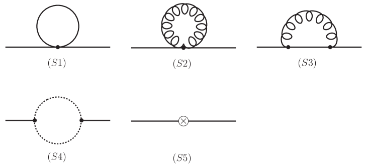
Figure 7: One-loop self-energy diagrams for the scalar fields. The solid lines are scalars, curly lines are gauge bosons, and dotted lines are Majorana fermions. The final diagram $(S5)$ denotes the wavefunction renormalization counterterm. The external lines are light modes with small spatial momenta, while the fields running inside the loops are heavy modes.

The lowest-order thermal mass correction for the scalar fields comes from the self-energy diagrams shown in Fig. 7. As noted in section 3, to extract the $\mathcal{O}(\lambda T^{2})$ contribution to the mass (squared), one may evaluate these diagrams in flat space and without chemical potentials. Including curvature and chemical potential corrections in these diagrams would give subleading $\mathcal{O}(\lambda^{2})$ terms, which are beyond the accuracy we need. Since we are interested in the construction of ESYM₃, only the heavy mode contributions to each loop should be included. To obtain the thermal mass, it is sufficient to evaluate these diagrams at zero external momentum. But we will keep the external (Euclidean) momentum $p=(0,\vec{p}\,)$ non-zero (but small compared to $T$) in order to extract the one-loop wavefunction renormalization for the scalars, which will be useful in the next subsection. We use dimensional continuation and the $\overline{MS}$ renormalization scheme, and denote the arbitrary renormalization scale by $\Lambda$. Integrals are carried out in the standard manner with the convention that

$$\sum\negthickspace{\negthickspace{\negthickspace{\negthickspace{\negthickspace{\int_{p}^{\,\prime}}}}}}\equiv\left(\frac{e^{\gamma_{E}}\Lambda^{2}}{4\pi}\right)^{\epsilon}T\sum_{n\neq 0}\int\frac{d^{3-2\epsilon}p}{(2\pi)^{3-2\epsilon}}\;.$$ (97)

The prime in the left-hand side signifies the omission of the zero frequency mode in bosonic loop integrals. We use a Lorentz gauge-fixing term with arbitrary gauge parameter $\alpha$. The dependence on $\alpha$ will drop out of the result for the thermal mass correction, but keeping $\alpha$ arbitrary serves as a useful check on the calculation.

Evaluating the diagrams of Fig. 7 is straightforward and one finds:

$$(S1) =-\frac{5}{12}\,\lambda T^{2}\,,$$ (98a)

$$(S2) =-\frac{1}{12}\,(3+\alpha)\,\lambda T^{2}\,,$$ (98b)

$$(S3) =\frac{\alpha}{12}\,\lambda T^{2}+\frac{\lambda}{16\pi^{2}}\,\Bigl{(}\frac{1}{\epsilon}+L_{b}\Bigr{)}\,(3{-}\alpha)\,p^{2}+\mathcal{O}\Bigl{(}\frac{p^{4}}{T^{2}}\Bigr{)}\,,$$ (98c)

$$(S4) =-\frac{1}{3}\,\lambda T^{2}-\frac{\lambda}{4\pi^{2}}\Bigl{(}\frac{1}{\epsilon}+L_{f}\Bigr{)}\,p^{2}+\mathcal{O}\Bigl{(}\frac{p^{4}}{T^{2}}\Bigr{)}\,,$$ (98d)

$$(S5) =-\delta Z^{(1)}\,p^{2}\,,$$ (98e)

where $\delta Z^{(1)}$ is the one-loop wavefunction renormalization counterterm. We have defined

$$L_{b}\equiv\ln\frac{\Lambda^{2}}{T^{2}}-2\ln(4\pi)+2\gamma_{E}\;,\quad L_{f}\equiv\ln\frac{\Lambda^{2}}{T^{2}}-2\ln(4\pi)+2\gamma_{E}+4\ln 2\;,$$ (99)

with $\gamma_{E}$ is Euler’s constant. The sum of these diagrams gives (minus) the hard mode contribution to the one-loop self-energy,

$$-\Pi_{\rm hard}(p) \equiv(S1)+(S2)+(S3)+(S4)+(S5)$$

$$=-\lambda T^{2}+p^{2}\frac{\lambda}{16\pi^{2}}\,\left\{(3{-}\alpha)L_{b}-4L_{f}-\frac{1{+}\alpha}{\epsilon}\right\}-p^{2}\,\delta Z^{(1)}+\mathcal{O}\Bigl{(}\frac{p^{4}}{T^{2}}\Bigr{)}\,.$$ (100)

Choosing

$$\delta Z^{(1)}=-(1+\alpha)\,\frac{\lambda}{16\pi^{2}\epsilon}$$ (101)

absorbs the logarithmic divergence. As always, temperature independent renormalization suffices to remove UV divergences at any temperature. The hard-mode self-energy is thus

$$-\Pi_{\rm hard}(p)=-\lambda T^{2}+p^{2}\frac{\lambda}{16\pi^{2}}\left\{(3{-}\alpha)L_{b}-4L_{f}\right\}+\mathcal{O}\Bigl{(}\frac{p^{4}}{T^{2}}\Bigr{)}\,.$$ (102)

The resulting renormalized scalar propagator, in flat space and without chemical potentials, at separations large compared to $1/T$, is

$$\langle\Phi_{A}(x)\Phi_{B}(y)\rangle=\delta_{AB}\>T\int\frac{d^{3}p}{(2\pi)^{3}}\>e^{i\vec{p}\cdot(\vec{x}-\vec{y})}\>G(p)\,,$$ (103)

with

$$G^{-1}(p) =p^{2}+\Pi_{\rm hard}(p)+\Pi_{\rm soft}(p)$$

$$=p^{2}(1+A)+\lambda\,T^{2}+\Pi_{\rm soft}(p)+\mathcal{O}(p^{4}/T^{2})+\mathcal{O}(\lambda^{2}T^{2})\,,$$ (104)

where $A\equiv-\frac{\lambda}{16\pi^{2}}\left\{(3{-}\alpha)L_{b}-4L_{f}\right\}$ and $\Pi_{\rm soft}(p)$ is the self-energy contribution due to soft modes.

In view of the relation (37), the long distance correlator (103) should be matched with $Z_{3}T\langle\tilde{\Phi}_{A}(x)\tilde{\Phi}_{B}(y)\rangle$, computed in the effective theory. Again neglecting curvature and chemical potential corrections, the effective theory correlator is

$$\langle\tilde{\Phi}_{A}(x)\tilde{\Phi}_{B}(y)\rangle=\delta_{AB}\,\int\frac{d^{3}p}{(2\pi)^{3}}\>e^{i\vec{p}\cdot(\vec{x}-\vec{y})}\>\widetilde{G}(p)\,,$$ (105)

with

$$\widetilde{G}^{-1}(p)=p^{2}+\delta m^{2}(T)+\Pi_{\rm soft}(p)\,,$$ (106)

and $\Pi_{\rm soft}(p)$ is the same soft mode contribution as in (B.2). Therefore, the parameters of the effective theory must be adjusted to make $\widetilde{G}^{-1}(p)/Z_{3}$ coincide with $G^{-1}(p)$. Through one-loop order, the required matching is

$$Z_{3}=(1+A)^{-1}=1+\frac{\lambda}{16\pi^{2}}\left\{(3{-}\alpha)L_{b}-4L_{f}\right\}+\mathcal{O}(\lambda^{2})\,,$$ (107)

and

$$\delta m^{2}(T)=\lambda\,T^{2}+\mathcal{O}(\lambda^{2}T^{2})\,.$$ (108)

B.3 Scalar Quartic Coupling

Calculating the one-loop thermal corrections to the scalar quartic interactions which will appear in the high temperature effective theory requires evaluation of the one-loop four-point correlator of light-mode scalar fields, at zero external momentum. The analysis is similar to the computation by Nadkarni [37] of the quartic interactions of $A_{0}$ in EQCD. The required diagrams are shown in Fig. 8. Once again, only heavy modes should be regarded as running around the loops, and one may work directly in flat space, ignoring curvature and chemical potential corrections.

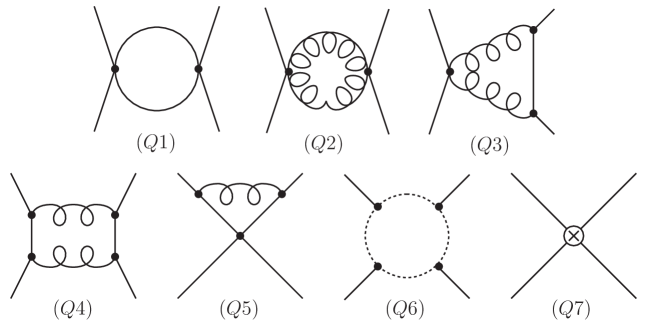
Figure 8: One loop diagrams which lead to quartic scalar interactions in the high temperature effective theory. As in Fig. 7, solid, curly, and dotted lines denote scalar, gauge boson, and fermion lines, respectively. In Diagram $(Q6)$, it is most convenient to treat the external fields $X$ and $Y$ separately due to their different Yukawa couplings. Diagram $(Q7)$ denotes the contribution induced by wavefunction renormalization. Not shown explicitly are the various permutations of each diagram.

We evaluate these diagrams using dimensional continuation and $\overline{MS}$ renormalization, as described in appendix B.2, and an arbitrary gauge fixing parameter $\alpha$, even though choosing Landau gauge ($\alpha\,{=}\,0$) would reduce the number of the diagrams to be computed (namely diagrams $(Q3)$, $(Q4)$, and $(Q5)$ would all vanish at zero external momentum). Nevertheless, retaining an arbitrary gauge fixing parameter in order to verify the cancellation of $\alpha$ dependence in the resulting effective quartic coupling serves as a useful consistency check.

To express the results compactly, we will use $\{V^{a}\}$ to denote Hermitian $SU(N_{c})$ adjoint representation basis matrices, with

$$(V^{a})_{bc}\equiv-if^{abc}\;,$$ (109)

and define the following index structures:

$$(\Gamma_{1})^{abcd}_{ABCD}\equiv N_{c}^{-2}\Bigl{[}\>\operatorname{tr}(V^{a}V^{b}V^{c}V^{d}) \,(\delta_{AB}\,\delta_{CD}+\delta_{AD}\,\delta_{BC}-2\delta_{AC}\,\delta_{BD})$$

$$+\operatorname{tr}(V^{a}V^{b}V^{d}V^{c}) \,(\delta_{AC}\,\delta_{BD}+\delta_{AB}\,\delta_{CD}-2\delta_{AD}\,\delta_{BC})$$

$$+\operatorname{tr}(V^{a}V^{c}V^{b}V^{d}) \,(\delta_{AC}\,\delta_{BD}+\delta_{AD}\,\delta_{BC}-2\delta_{AB}\,\delta_{CD})\Bigr{]}\;,$$ (110a)

$$(\Gamma_{2})^{abcd}_{ABCD}\equiv N_{c}^{-2}\Bigl{[}\>\operatorname{tr}(V^{a}V^{b}V^{c}V^{d}) \,(\delta_{AB}\,\delta_{CD}+\delta_{AD}\,\delta_{BC})$$

$$+\operatorname{tr}(V^{a}V^{b}V^{d}V^{c}) \,(\delta_{AC}\,\delta_{BD}+\delta_{AB}\,\delta_{CD})$$

$$+\operatorname{tr}(V^{a}V^{c}V^{b}V^{d}) \,(\delta_{AC}\,\delta_{BD}+\delta_{AD}\,\delta_{BC})\Bigr{]}\;.$$ (110b)

The tree-level quartic scalar vertex is $-2\,\lambda\,(\Gamma_{1})^{abcd}_{ABCD}\,$.

The diagrams of Figure 8 can be computed in a straightforward manner, and one finds

$$(Q1) =\frac{\lambda^{2}}{16\pi^{2}}\,\Bigl{(}\frac{1}{\epsilon}+L_{b}\Bigr{)}\left[4(\Gamma_{1})^{abcd}_{ABCD}+5(\Gamma_{2})^{abcd}_{ABCD}\right],$$ (112a)

$$(Q2) =(3+\alpha^{2})\,\frac{\lambda^{2}}{16\pi^{2}}\,\Bigl{(}\frac{1}{\epsilon}+L_{b}\Bigr{)}\,(\Gamma_{2})^{abcd}_{ABCD}\;,$$ (112b)

$$(Q3) =-2\alpha^{2}\,\frac{\lambda^{2}}{16\pi^{2}}\,\Bigl{(}\frac{1}{\epsilon}+L_{b}\Bigr{)}\,(\Gamma_{2})^{abcd}_{ABCD}\;,$$ (112c)

$$(Q4) =\alpha^{2}\,\frac{\lambda^{2}}{16\pi^{2}}\,\Bigl{(}\frac{1}{\epsilon}+L_{b}\Bigr{)}\,(\Gamma_{2})^{abcd}_{ABCD}\;,$$ (112d)

$$(Q5) =-4\alpha\,\frac{\lambda^{2}}{16\pi^{2}}\,\Bigl{(}\frac{1}{\epsilon}+L_{b}\Bigr{)}\,(\Gamma_{1})^{abcd}_{ABCD}\;,$$ (112e)

$$(Q6) =-8\,\frac{\lambda^{2}}{16\pi^{2}}\,\Bigl{(}\frac{1}{\epsilon}+L_{f}\Bigr{)}\,\left[(\Gamma_{1})^{abcd}_{ABCD}+(\Gamma_{2})^{abcd}_{ABCD}\right],$$ (112f)

$$(Q7) =-4\lambda\>\delta Z^{(1)}\,(\Gamma_{1})^{abcd}_{ABCD}\;.$$ (112g)

Diagram $(Q6)$ requires a special attention because the $X_{p}$ and $Y_{p}$ scalars have different Yukawa couplings. Considering the various cases (such as $\langle X^{a}_{p}\,X^{b}_{q}\,Y^{c}_{r}\,Y^{d}_{s}\rangle$) and taking care of the appropriate permutations, one finds the simple expression above. Inserting the previously determined one-loop scalar wavefunction renormalization factor $\delta Z^{(1)}$ [from Eq. (101)] into the result $(Q7)$ gives

$$(Q7)=4\,\frac{\lambda^{2}}{16\pi^{2}\epsilon}\,(1+\alpha)\,(\Gamma_{1})^{abcd}_{ABCD}\;.$$ (113)

Combining all terms, we find that the amputated 1PI scalar 4-point function, at zero momentum, is

$$\langle\Phi_{A}^{a}\Phi_{B}^{b}\Phi_{C}^{c}\Phi_{D}^{d}\rangle_{\rm 1PI} =(\Gamma_{1})^{abcd}_{ABCD}\,\Bigl{(}-2\,\lambda\,+\frac{\lambda^{2}}{4\pi^{2}}[(1{-}\alpha)L_{b}-2L_{f}]\Bigr{)}$$

$$+(\Gamma_{2})^{abcd}_{ABCD}\>\frac{\lambda^{2}}{2\pi^{2}}\>[L_{b}-L_{f}]+\mathcal{O}(\lambda^{3})\;.$$ (114)

Rescaling the field according to relations (37) and (107) removes the remaining gauge fixing parameter dependence and produces the equivalent ESYM₃ 1PI 4-point function,

$$\langle\tilde{\Phi}_{A}^{a}\tilde{\Phi}_{B}^{b}\tilde{\Phi}_{C}^{c}\tilde{\Phi}_{D}^{d}\rangle_{\rm 1PI} =-2\lambda T^{2}\,(\Gamma_{1})^{abcd}_{ABCD}-(\ln 4)\,\frac{\lambda^{2}T^{2}}{\pi^{2}}\left[(\Gamma_{2})^{abcd}_{ABCD}-(\Gamma_{1})^{abcd}_{ABCD}\right]+\mathcal{O}(\lambda^{3})\;.$$ (115)

The first term is the vertex which arises from the commutator squared interaction directly inherited from the full theory, while the order $\lambda^{2}$ correction comes out to be remarkably simple. Both terms must be produced as tree level vertices in the three-dimensional effective theory. The required quartic interaction terms in the ESYM₃ effective Lagrangian are

$${\textstyle\frac{1}{2}}g_{3}^{2}\,\operatorname{tr}(i[\tilde{\Phi}_{A},\tilde{\Phi}_{B}])^{2}+\frac{\ln 2}{2\pi^{2}}\,\frac{g_{3}^{4}}{T}\,\operatorname{tr}(\tilde{\Phi}^{a}_{A}V_{a}\tilde{\Phi}^{b}_{B}V_{b})^{2}\,,$$ (116)

with $g_{3}^{2}\equiv g^{2}T$. All gauge fixing parameter dependence and $1/\epsilon$ poles have canceled, as required. The $\ln(\Lambda^{2}/T^{2})$ terms in $L_{b}$ and $L_{f}$ have also dropped out. This was also required, since $\mathcal{N}\,{=}\,4$ SYM at zero temperature is a conformal theory in which the coupling does not run, and turning on a temperature does not change the short distance behavior.

Appendix C Background Field Method

We wish to evaluate the complete one-loop effective potential for the scalar fields using background field techniques. We will restrict our analysis to the special case where the background scalar fields take values along flat directions of the tree-level potential. This is sufficient for our purposes, and simplifies the calculation. We carry out the calculations in flat space, and neglect chemical potentials. Under our assumptions that $1/R^{2}$ and $\mu^{2}$ are both of order $\lambda T^{2}$, the tree-level contributions from the curvature and chemical potential induced mass terms will be comparable to one-loop corrections to the effective potential computed in flat space with $\mu=0$. Including curvature and chemical potential corrections in the evaluation of the one-loop potential would change the result by an amount comparable to neglected two-loop contributions.

In the flat space Lagrangian, shown in Eq. (2.2) but without mass and chemical potential terms, we shift the scalar fields by constants,

$$\Phi_{A}\rightarrow\bar{\Phi}_{A}+\sigma_{A}\;,$$ (117)

with $\bar{\Phi}_{A}$ constant fields taking values in the flat directions, and $\sigma_{A}$, are arbitrary fluctuations about the constant background. The background fields (viewed as $N_{c}\times N_{c}$ matrices) are simultaneously diagonal (up to an irrelevant gauge transformation).

Among the quadratic terms in the shifted Lagrangian, there are terms which mix the gauge and scalar fields. These may be eliminated by employing the $R_{\xi}$-gauge with gauge-fixing term

$$\frac{1}{\xi}\operatorname{tr}\!\left\{(\partial_{\mu}A_{\mu}-i\xi\,g[\sigma_{A},\bar{\Phi}_{A}])^{2}\right\}\;.$$ (118)

We further set $\xi=1$ to simplify the computation, as this choice eliminates off-diagonal quadratic terms which mix $\sigma_{A}$ and $\sigma_{B}$ for $A\neq B$. We denote the matrix components of the fields by indices $m$ and $n$ so that, for example, $(\sigma_{A})_{mn}\equiv\sum_{a}\sigma_{A}^{a}(T^{a})_{mn}$.

Let $\lambda^{m}_{A}$ denote the $m$th eigenvalue of the constant background field $\bar{\Phi}_{A}$ and define, for convenience,

$$M^{2}_{mn}\equiv g^{2}\sum_{A}\>(\lambda^{m}_{A}-\lambda^{n}_{A})^{2}\;.$$ (119)

Note that $m$ and $n$ are not to be summed over in the definition of $M_{mn}^{2}$. The resulting quadratic terms in the shifted Lagrangian are

$$\sum_{m,n}\bigg{[} (A_{\mu})^{*}_{mn}\left(-\partial^{2}+M_{mn}^{2}\right)(A_{\mu})_{mn}+(\sigma_{A})^{*}_{mn}\left(-\partial^{2}+M_{mn}^{2}\right)(\sigma_{A})_{mn}$$

$$+(\bar{\psi_{i}})_{mn}\left[\delta_{ij}\,i{\partial}\negthickspace{\negthickspace{/}}-g\left\{\alpha^{p}_{ij}+i\gamma_{5}\,\beta^{p}_{ij}\right\}(\lambda^{m}_{p}{-}\lambda^{n}_{p})\right](\psi_{j})_{mn}\bigg{]}\,.$$ (120)

In carrying out the Gaussian integrals, one finds that the logarithms of the functional determinants from all the three contributions simplify to the generic form

$$I=\sum\negthickspace{\negthickspace{\negthickspace{\negthickspace{\negthickspace{\int_{p}^{\,\prime}}}}}}\ln(p^{2}+M_{mn}^{2})\;,$$ (121)

where the sum-integral is defined in Eq. (97). This integral is standard after Arnold and Espinosa [38], and yields

$$\frac{I_{\text{bose}}}{\pi^{2}T^{4}} =-{\textstyle\frac{1}{45}}+{\textstyle\frac{1}{3}}\Big{(}\frac{M_{mn}^{2}}{4\pi^{2}T^{2}}\!\Big{)}-{\textstyle\frac{1}{2}}\Big{(}\frac{1}{\epsilon}{+}L_{b}\!\Big{)}\!\Big{(}\frac{M_{mn}^{2}}{4\pi^{2}T^{2}}\!\Big{)}^{2}-\sum_{l=3}^{\infty}8\,\frac{(2l{-}5)!!}{(2l)!!}\,\zeta(2l{-}3)\Big{(}\frac{-M_{mn}^{2}}{4\pi^{2}T^{2}}\!\Big{)}^{l}\,,$$ (122a)

$$\frac{I_{\text{fermi}}}{\pi^{2}T^{4}} ={\textstyle\frac{7}{360}}-{\textstyle\frac{1}{6}}\Big{(}\frac{M_{mn}^{2}}{4\pi^{2}T^{2}}\!\Big{)}-{\textstyle\frac{1}{2}}\Big{(}\frac{1}{\epsilon}{+}L_{f}\!\Big{)}\!\Big{(}\frac{M_{mn}^{2}}{4\pi^{2}T^{2}}\!\Big{)}^{2}-\!\sum_{l=3}^{\infty}(4^{l}{-}8)\frac{(2l{-}5)!!}{(2l)!!}\,\zeta(2l{-}3)\Big{(}\frac{-M_{mn}^{2}}{4\pi^{2}T^{2}}\!\Big{)}^{l},$$ (122b)

where $I_{\text{bose}}$ and $I_{\text{fermi}}$ are contributions from the bosons and fermions, respectively. In these results, $\mathcal{O}(\epsilon)$ terms have been discarded and the quantities $L_{b}$ and $L_{f}$ are defined in Eq. (99).

For each color component, the gauge field, six scalar fields, and gauge fixing ghosts contribute $(4+6-2)=8$ times ${\textstyle\frac{\beta}{2}}I_{\rm bose}$ to the (three dimensional) effective potential, while the fermions contribute $-8$ times ${\textstyle\frac{\beta}{2}}I_{\rm fermi}$. The resulting effective potential, for background fields lying along flat directions, is thus

$$\overline{V}(\bar{\Phi}_{A})={\textstyle\frac{1}{2}}\pi^{2}T^{3}\sum_{m,n}\bigg{[}\,-\frac{1}{3} +\left(\frac{M_{mn}^{2}}{\pi^{2}T^{2}}\right)+(\ln 2)\left(\frac{M_{mn}^{2}}{\pi^{2}T^{2}}\right)^{2}$$

$$+\sum_{l=3}^{\infty}\>8\,(1-4^{-l+2})\,\frac{(2l{-}5)!!}{(2l)!!}\,\zeta(2l{-}3)\left(-\frac{M_{mn}^{2}}{\pi^{2}T^{2}}\right)^{l}\,\bigg{]}\;.$$ (123)

The $1/\epsilon$ poles and all dependence on the arbitrary renormalization scale has canceled, as required for a physical quantity.

We would like to express the result (C) in terms of the original fields $\bar{\Phi}_{A}$. To do so, note that the adjoint representation of the field, $(\bar{\Phi}_{A}^{\text{adj}})_{ab}\equiv i\bar{\Phi}_{A}^{b}f^{abc}$, may also be written as

$$(\bar{\Phi}_{A}^{\text{adj}})_{ab}=2\operatorname{tr}(T_{a}[\bar{\Phi}_{A},T_{b}])\;.$$ (124)

Since the fields $\bar{\Phi}_{A}$ are assumed to take values in flat directions, a Cartan subalgebra may chosen for which $\bar{\Phi}_{A}$ is diagonal with the entries $\lambda_{A}^{m}$. Therefore

$$\operatorname{tr}(\bar{\Phi}_{A}^{\text{adj}}\bar{\Phi}_{B}^{\text{adj}}) =2\sum_{a}\operatorname{tr}(T_{a}[\bar{\Phi}_{A},[\bar{\Phi}_{B},T_{a}]])$$

$$=2\sum_{a,m,n}(T_{a})_{nm}(\lambda_{A}^{m}{-}\lambda_{A}^{n})(\lambda_{B}^{m}{-}\lambda_{B}^{n})(T_{a})_{mn}$$

$$=\sum_{m,n}\>(\lambda_{A}^{m}{-}\lambda_{A}^{n})(\lambda_{B}^{m}{-}\lambda_{B}^{n})\,,$$ (125)

where the last step used the identity $\sum_{a}(T_{a})_{ij}(T_{a})_{kl}=\frac{1}{2}\,(\delta_{il}\delta_{jk}-\frac{1}{N_{c}}\,\delta_{ij}\delta_{kl})$. Hence $\operatorname{tr}[g^{2}\sum_{A}\bar{\Phi}_{A}^{\text{adj}}\bar{\Phi}_{A}^{\text{adj}}]=g^{2}\sum_{A,m,n}(\lambda_{A}^{m}{-}\lambda_{A}^{n})^{2}=\sum_{m,n}M_{mn}^{2}$. Since the sum of the eigenvalues $\lambda_{A}^{m}$ must vanish (because $\bar{\Phi}_{A}$ is traceless), this may also be written in the form

$${\textstyle\frac{1}{2}}g^{2}T^{2}\operatorname{tr}(\bar{\Phi}_{A}^{\text{adj}}\bar{\Phi}_{A}^{\text{adj}})={\textstyle\frac{1}{2}}T^{2}\sum_{m,n}M_{mn}^{2}=g^{2}T^{2}N_{c}\sum_{A,m}(\lambda_{A}^{m})^{2}=\lambda T^{2}\operatorname{tr}(\bar{\Phi}_{A})^{2}\;,$$ (126)

which shows that the quadratic part of the effective potential (C) agrees with the previously derived thermal mass correction (42). [Note that, to the lowest order, the rescaling from $\Phi_{A}$ to $\tilde{\Phi}_{A}$ in (37) is just a factor of $\sqrt{T}$.] More generally, we have

$$\operatorname{tr}\Big{[}\Big{(}g^{2}\sum_{A}\bar{\Phi}_{A}^{\text{adj}}\bar{\Phi}_{A}^{\text{adj}}\Big{)}^{l}\Big{]}=\sum_{m,n}\>\left(M_{mn}^{2}\right)^{l}\;,$$ (127)

so the effective potential (C) (along flat directions) may be expressed in terms of adjoint representation traces as shown in Eq. (47). In particular, the quartic term of (C) is $\frac{\beta}{2\pi^{2}}\,(\ln 2)\,g^{4}\operatorname{tr}[(\bar{\Phi}^{\text{adj}}_{A}\bar{\Phi}^{\text{adj}}_{A})^{2}]$ and this agrees, for commuting fields, with the diagrammatic result (116).

References

- [1] G. ’t Hooft, A Planar Diagram Theory For Strong Interactions, Nucl. Phys. B 72, 461 (1974).
- [2] L. G. Yaffe, Large Limits As Classical Mechanics, Rev. Mod. Phys. 54, 407 (1982).
- [3] G. Veneziano, Some Aspects Of A Unified Approach To Gauge, Dual And Gribov Theories, Nucl. Phys. B 117, 519 (1976).
- [4] E. Witten, Baryons In The 1/N Expansion, Nucl. Phys. B 160, 57 (1979).
- [5] D. J. Gross and E. Witten, Possible Third Order Phase Transition In The Large N Lattice Gauge Theory, Phys. Rev. D 21, 446 (1980).
- [6] B. Sundborg, The Hagedorn transition, deconfinement and = 4 SYM theory, Nucl. Phys. B 573, 349 (2000) [arXiv:hep-th/9908001].
- [7] O. Aharony, J. Marsano, S. Minwalla, K. Papadodimas and M. Van Raamsdonk, The Hagedorn / deconfinement phase transition in weakly coupled large N gauge theories, arXiv:hep-th/0310285.
- [8] O. Aharony, J. Marsano, S. Minwalla, K. Papadodimas and M. Van Raamsdonk, A first order deconfinement transition in large N Yang-Mills theory on a small S**3, arXiv:hep-th/0502149.
- [9] J. M. Maldacena, The large N limit of superconformal field theories and supergravity, Adv. Theor. Math. Phys. 2, 231 (1998) [Int. J. Theor. Phys. 38, 1113 (1999)] [arXiv:hep-th/9711200].
- [10] S. S. Gubser, I. R. Klebanov and A. M. Polyakov, Gauge theory correlators from non-critical string theory, Phys. Lett. B 428, 105 (1998) [arXiv:hep-th/9802109].
- [11] E. Witten, Anti-de Sitter space and holography, Adv. Theor. Math. Phys. 2, 253 (1998) [arXiv:hep-th/9802150].
- [12] S. W. Hawking and D. N. Page, Thermodynamics Of Black Holes In Anti-De Sitter Space, Commun. Math. Phys. 87, 577 (1983).
- [13] E. Witten, Anti-de Sitter space, thermal phase transition, and confinement in gauge theories, Adv. Theor. Math. Phys. 2, 505 (1998) [arXiv:hep-th/9803131].
- [14] K. Behrndt, M. Cvetic and W. A. Sabra, Non-extreme black holes of five dimensional N = 2 AdS supergravity, Nucl. Phys. B 553, 317 (1999) [arXiv:hep-th/9810227].
- [15] G. W. Gibbons and S. W. Hawking, Action Integrals And Partition Functions In Quantum Gravity, Phys. Rev. D 15, 2752 (1977).
- [16] V. Balasubramanian and P. Kraus, A stress tensor for anti-de Sitter gravity, Commun. Math. Phys. 208, 413 (1999) [arXiv:hep-th/9902121].
- [17] A. Chamblin, R. Emparan, C. V. Johnson and R. C. Myers, Charged AdS black holes and catastrophic holography, Phys. Rev. D 60, 064018 (1999) [arXiv:hep-th/9902170].
- [18] M. Cvetic and S. S. Gubser, Phases of R-charged black holes, spinning branes and strongly coupled gauge theories, JHEP 9904, 024 (1999) [arXiv:hep-th/9902195].
- [19] S. S. Gubser and I. Mitra, The evolution of unstable black holes in anti-de Sitter space, JHEP 0108, 018 (2001) [arXiv:hep-th/0011127].
- [20] S. S. Gubser, Thermodynamics of spinning D3-branes, Nucl. Phys. B 551, 667 (1999) [arXiv:hep-th/9810225].
- [21] S. W. Hawking and H. S. Reall, Charged and rotating AdS black holes and their CFT duals, Phys. Rev. D 61, 024014 (2000) [arXiv:hep-th/9908109].
- [22] P. Basu and S. R. Wadia, R-charged AdS(5) black holes and large N unitary matrix models, Phys. Rev. D 73, 045022 (2006) [arXiv:hep-th/0506203].
- [23] A. M. Polyakov, Gauge fields and space-time, Int. J. Mod. Phys. A 17S1, 119 (2002) [arXiv:hep-th/0110196].
- [24] H. E. Haber and H. A. Weldon, Finite Temperature Symmetry Breaking As Bose-Einstein Condensation, Phys. Rev. D 25, 502 (1982).
- [25] F. Gliozzi, J. Scherk and D. I. Olive, Supersymmetry, Supergravity Theories And The Dual Spinor Model, Nucl. Phys. B 122, 253 (1977).
- [26] L. Brink, J. H. Schwarz and J. Scherk, Supersymmetric Yang-Mills Theories, Nucl. Phys. B 121, 77 (1977).
- [27] T. Appelquist and J. Carazzone, Infrared Singularities And Massive Fields, Phys. Rev. D 11, 2856 (1975).
- [28] D. J. Gross, R. D. Pisarski and L. G. Yaffe, QCD And Instantons At Finite Temperature, Rev. Mod. Phys. 53, 43 (1981).
- [29] E. Braaten and A. Nieto, Effective field theory approach to high temperature thermodynamics, Phys. Rev. D 51, 6990 (1995) [arXiv:hep-ph/9501375].
- [30] E. Braaten and A. Nieto, Free Energy of QCD at High Temperature, Phys. Rev. D 53, 3421 (1996) [arXiv:hep-ph/9510408].
- [31] C. j. Kim and S. J. Rey, Thermodynamics of large-N super Yang-Mills theory and AdS/CFT correspondence, Nucl. Phys. B 564, 430 (2000) [arXiv:hep-th/9905205].
- [32] A. Fotopoulos and T. R. Taylor, Comment on two-loop free energy in = 4 supersymmetric Yang-Mills theory at finite temperature, Phys. Rev. D 59, 061701 (1999) [arXiv:hep-th/9811224].
- [33] M. A. Vazquez-Mozo, A note on supersymmetric Yang-Mills thermodynamics, Phys. Rev. D 60, 106010 (1999) [arXiv:hep-th/9905030].
- [34] E. Gava and R. Jengo, Perturbative Evaluation Of The Thermal Wilson Loop, Phys. Lett. B 105, 285 (1981).
- [35] S. R. Coleman, The Fate Of The False Vacuum. 1. Semiclassical Theory, Phys. Rev. D 15, 2929 (1977) [Erratum-ibid. D 16, 1248 (1977)].
- [36] C. G. Callan and S. R. Coleman, The Fate Of The False Vacuum. 2. First Quantum Corrections, Phys. Rev. D 16, 1762 (1977).
- [37] S. Nadkarni, Dimensional Reduction In Finite Temperature Quantum Chromodynamics. 2, Phys. Rev. D 38, 3287 (1988).
- [38] P. Arnold and O. Espinosa, The effective potential and first order phase transitions: Beyond leading-order, Phys. Rev. D 47, 3546 (1993) [Erratum-ibid. D 50, 6662 (1994)] [arXiv:hep-ph/9212235].