Taub-NUT/Bolt Black Holes in Gauss-Bonnet-Maxwell Gravity

Abstract

We present a class of higher dimensional solutions to Gauss-Bonnet-Maxwell equations in $2k+2$ dimensions with a $U(1)$ fibration over a $2k$-dimensional base space $\mathcal{B}$. These solutions depend on two extra parameters, other than the mass and the NUT charge, which are the electric charge $q$ and the electric potential at infinity $V$. We find that the form of metric is sensitive to geometry of the base space, while the form of electromagnetic field is independent of $\mathcal{B}$. We investigate the existence of Taub-NUT/bolt solutions and find that in addition to the two conditions of uncharged NUT solutions, there exist two other conditions. These two extra conditions come from the regularity of vector potential at $r=N$ and the fact that the horizon at $r=N$ should be the outer horizon of the black hole. We find that for all non-extremal NUT solutions of Einstein gravity having no curvature singularity at $r=N$, there exist NUT solutions in Gauss-Bonnet-Maxwell gravity. Indeed, we have non-extreme NUT solutions in $2+2k$ dimensions only when the $2k$-dimensional base space is chosen to be $\mathbb{CP}^{2k}$. We also find that the Gauss-Bonnet-Maxwell gravity has extremal NUT solutions whenever the base space is a product of 2-torii with at most a $2$-dimensional factor space of positive curvature, even though there a curvature singularity exists at $r=N$. We also find that one can have bolt solutions in Gauss-Bonnet-Maxwell gravity with any base space. The only case for which one does not have black hole solutions is in the absence of a cosmological term with zero curvature base space.

I Introduction

The prominence of string theory as a theory of everything, in particular a quantum theory of gravity, means that we should examine its consequences in regimes where it departs from the Einstein gravity. One way of examining the consequence of string theory on the solutions of classical gravity is through the use of the field equations which arise from the effective action of a low-energy limit of string theory. This effective action which describes gravity at the classical level consists of the Einstein-Hilbert action plus curvature-squared terms and higher powers as well, and in general give rise to fourth order field equations and bring in ghosts Wit1 . However, if the effective action contains the higher powers of curvature in particular combinations, then only second order field equations are produced and consequently no ghosts arise Zum . The effective action obtained by this argument is precisely of the form proposed by Lovelock Lov . It is therefore natural to suppose that the construction of the Taub-Nut solutions of Gauss-Bonnet gravity, which is the first order corrections of the string theory at low energy, might provide us with a window on some interesting new corners of this theory. The first attempt has been done by one of us, and the Taub-NUT/bolt solutions of Gauss-Bonnet gravity have been constructed Deh1 . These solutions have some features which are different from the Nut solutions of Einstein gravity. Here, we construct the Taub-NUT solutions in Gauss-Bonnet-Maxwell gravity and investigate their properties.

In the last decades a renewed interest appears in Lovelock gravity. In particular, exact static spherically symmetric black hole solutions of the Gauss-Bonnet gravity have been found in Ref. Des , and of the Maxwell-Gauss-Bonnet and Born-Infeld-Gauss-Bonnet models in Ref. Wil1 . The thermodynamics of the uncharged static spherically black hole solutions has been considered in MS , of solutions with nontrivial topology in Cai and of charged solutions in Wil1 ; Od1 . All of these known solutions in Gauss-Bonnet gravity are static. Recently one of us has introduced two new classes of rotating solutions of second order Lovelock gravity and investigate their thermodynamics Deh2 . Also, the exact solutions in third order Lovelock gravity with the quartic terms has been constructed recently Deh3 .

The original four-dimensional solution TNUT is only locally asymptotic flat. The spacetime has as a boundary at infinity a twisted $S^{1}$ bundle over $S^{2}$, instead of simply being $S^{1}\times S^{2}$. In general, the Killing vector that corresponds to the coordinate that parameterizes the fibre $S^{1}$ can have a zero-dimensional fixed point set (called a NUT solution) or a two-dimensional fixed point set (referred to as a ‘bolt’ solution). There are known extensions of the Taub-NUT/bolt solutions to the case when a cosmological constant is present. In this case the asymptotic structure is only locally de Sitter (for positive cosmological constant) or anti-de Sitter (for negative cosmological constant) and the solutions are referred to as Taub-NUT-(A)dS metrics. Generalizations to higher dimensions follow closely the four-dimensional case Bais ; Page ; Akbar ; Robinson ; Awad ; Lorenzo ; Mann1 ; Mann2 ; Astefan1 ; Astefan2 . Also, charged Taub-NUT solution of the Einstein-Maxwell equations in four dimensions is known Bril , and its generalization to six dimensions has been done in Refs. Mann3 ; Awad2 . The existence of NUT charged solutions of Einstein-Yang-Mills and Einstein-Yang-Mills-Higgs theory and their thermodynamics have also been considered Radu . Dyonic Taub-NUT solution in the low energy limit of string theory has also been investigated Myers1 .

In this paper we consider Taub-NUT solutions in Gauss-Bonnet-Maxwell gravity in $2k+2$ dimensions. We find that NUT black holes exist, but Gauss-Bonnet-Maxwell gravity introduces some features not present in higher-dimensional Einstein-Maxwell gravity or Gauss-Bonnet gravity in the absence of electromagnetic field. The form of the metric function is sensitive to the base space over which the circle is fibred, while the form of the electromagnetic field is independent of the base space. We find that there exist some restrictions on the value of electric charge in order to have NUT solutions. Furthermore, we confirm the two conjectures of Ref. Deh1 and show that these conjectures can be extended to the case of Gauss-Bonnet gravity in the presence of electromagnetic field. Indeed, we show that pure non-extreme NUT solutions only exist if the base space has a single factor of maximal dimensionality, and extreme NUT solutions exist if the base space has at most one 2-dimensional curved space with positive curvature as one of its factor spaces.

The outline of our paper is as follows. We give a brief review of the field equations of second order Lovelock gravity in the presence of electromagnetic field in Sec. II. In Sec. III, we obtain all possible Taub-NUT/bolt solutions of Gauss-Bonnet-Maxwell gravity in six dimensions. Then, in Secs. IV and V, we present all kind of Taub-NUT/bolt solutions of Gauss-Bonnet-Maxwell gravity in eight and ten dimensions. In Sec VI, we extend our study to the $(2k+2)$-dimensional case. We finish our paper with some concluding remarks.

II Field Equations

The most natural extension of general relativity in higher dimensional spacetimes with the assumption of Einstein – that the left hand side of the field equations is the most general symmetric conserved tensor containing no more than second derivatives of the metric – is Lovelock theory. The gravitational action of this theory can be written as Lov

$$I_{G}=\int d^{d}x\sqrt{-g}\sum_{n=0}^{[d/2]}\alpha_{k}{\cal L}_{k}$$ (1)

where $[z]$ denotes the integer part of $z$, $\alpha_{k}$ is an arbitrary constant and ${\cal L}_{k}$ is the Euler density of a $2k$-dimensional manifold,

$${\cal L}_{k}=\frac{1}{2^{k}}\delta_{\rho_{1}\sigma_{1}\cdots\rho_{k}\sigma_{k}}^{\mu_{1}\nu_{1}\cdots\mu_{k}\nu_{k}}R_{\mu_{1}\nu_{1}}^{\phantom{\mu_{1}\nu_{1}}{\rho_{1}\sigma_{1}}}\cdots R_{\mu_{k}\nu_{k}}^{\phantom{\mu_{k}\nu_{k}}{\rho_{k}\sigma_{k}}}$$ (2)

In Eq. (2) $\delta_{\rho_{1}\sigma_{1}\cdots\rho_{k}\sigma_{k}}^{\mu_{1}\nu_{1}\cdots\mu_{k}\nu_{k}}$ is the generalized totally anti-symmetric Kronecker delta and $R_{\mu\nu}^{\phantom{\mu\nu}{\rho\sigma}}$ is the Riemann tensor. We note that in $d$ dimensions, all terms for which $n>[d/2]$ are identically equal to zero, and the term $n=d/2$ is a topological term. Consequently only terms for which $n<d/2$ contribute to the field equations. Here we study Gauss-Bonnet gravity, that is first three terms of Lovelock gravity. In this case the action is

$$I_{G}=\frac{1}{2}\int_{{\cal M}}d^{d}x\sqrt{-g}[-2\Lambda+R+\alpha(R_{\mu\nu\gamma\delta}R^{\mu\nu\gamma\delta}-4R_{\mu\nu}R^{\mu\nu}+R^{2})-F_{\mu\nu}F^{\mu\nu}]$$ (3)

where $\Lambda$ is the cosmological constant, $\alpha$ is the Gauss-Bonnet coefficient with dimension $({\rm length})^{2}$, $R$ and $R_{\mu\nu}$ are the Ricci scalar and Ricci tensors of the spacetime, $F_{\mu\nu}=\partial_{\mu}A_{\nu}-\partial_{\nu}A_{\mu}$ is electromagnetic tensor field and $A_{\mu}$ is the vector potential. Since $\alpha$ is positive in heterotic string theory Des we shall restrict ourselves to the case $\alpha>0$. The first term is the cosmological term, the second term is just the Einstein term, and the third term is the second order Lovelock (Gauss-Bonnet) term. From a geometric point of view the combination of these terms in five and six dimensions is the most general Lagrangian that yields second order field equations, as in the four-dimensional case for which the Einstein-Hilbert action is the most general Lagrangian producing second order field equations.

Varying the action with respect to the metric tensor $g_{\mu\nu}$ and electromagnetic tensor field $F_{\mu\nu}$ the equations of gravitation and electromagnetic fields are obtained as:

$$G_{\mu\nu}+\Lambda g_{\mu\nu}-\alpha\{4R^{\rho\sigma}R_{\mu\rho\nu\sigma}-2R_{\mu}^{\ \rho\sigma\lambda}R_{\nu\rho\sigma\lambda}-2RR_{\mu\nu}+4R_{\mu\lambda}R_{\text{ \ }\nu}^{\lambda}$$

$$+\frac{1}{2}g_{\mu\nu}(R_{\kappa\lambda\rho\sigma}R^{\kappa\lambda\rho\sigma}-4R_{\rho\sigma}R^{\rho\sigma}+R^{2})\}=T_{\mu\nu}$$ (4)

$$\nabla_{\mu}F^{\mu\nu}=0$$ (5)

where $G_{\mu\nu}$ is the Einstein tensor and $T_{\mu\nu}=2F_{\phantom{\lambda}{\mu}}^{\rho}F_{\rho\nu}-\frac{1}{2}F_{\rho\sigma}F^{\rho\sigma}g_{\mu\nu}$ is the energy-momentum tensor of electromagnetic field.

Since the second Lovelock term in Eq. (3) is an Euler density in four dimensions and has no contribution to the field equations in four or less dimensional spacetimes, and we seek Taub-NUT/bolt solutions in even dimensions, we therefore consider $(2k+2)$-dimensional spacetimes with $k\geq 2$. In constructing these metrics the idea is to regard the Taub-NUT spacetime as a $U(1)$ fibration over a $2k$-dimensional base space endowed with an Einstein-Kähler metric $g_{{\cal B}}$. Then the Euclidean section of the $(2k+2)$-dimensional Taub-NUT spacetime can be written as:

$$ds^{2}=F(r)(d\tau+N{\cal A})^{2}+F^{-1}(r)dr^{2}+(r^{2}-N^{2})g_{{\cal B}}$$ (6)

where $\tau$ is the coordinate on the fibre $S^{1}$ and ${\cal A}$ has a curvature $F=d{\cal A}$, which is proportional to some covariant constant 2-form. Here $N$ is the NUT charge and $F(r)$ is a function of $r$. The solution will describe a ‘NUT’ if the fixed point set of the $U(1)$ isometry $\partial/\partial\tau$ (i.e. the points where $F(r)=0$) is less than $2k$-dimensional and a ‘bolt’ if the fixed point set is $2k$-dimensional. We assume the following form for the vector potential $A$ Awad2

$$A=h(r)(d\tau+N{\cal A})$$ (7)

where ${\cal A}$ is the Kähler form of the base space ${\cal B}$ and $h(r)$ is an arbitrary function of $r$ which depends on the dimension of the spacetime and is independent of the base space ${\cal B}$. In this paper we construct the Taub-NUT/bolt solutions of Gauss-Bonnet gravity in the presence of electromagnetic field and extend the two conjectures of Ref. Deh1 to the case of electrically charged NUT solutions. These two conjectures were: 1) For all non-extremal NUT solutions of Einstein gravity having no curvature singularity at $r=N$, there exist NUT solutions in Gauss-Bonnet gravity that contain these solutions in the limit that the Gauss-Bonnet parameter $\alpha$ vanishes. 2) Gauss-Bonnet gravity has extremal NUT solutions whenever the base space is a product of $2$-torii with at most one $2$-dimensional space of positive curvature.

Here, we consider only the cases where all the factor spaces of ${\cal B}$ have zero or positive curvature. Thus, the base space ${\cal B}$ may be the product of $2$-sphere $S^{2}$, $2$-torus $T^{2}$ or ${\mathbb{C}P}^{k}$. For completeness, we give the $1$-forms and the metrics of these factor spaces. The $1$-forms and metrics of $S^{2}$, $T^{2}$ and ${\mathbb{C}P}^{k}$ are

$${\cal A}_{i} = 2\cos\theta_{i}d\phi_{i},$$

$$d\Omega^{2} = d\theta_{i}^{2}+\sin^{2}\theta_{i}d\phi_{i}^{2}$$

$${\cal A}_{i} = 2\eta_{i}d\zeta_{i}$$

$$d\Gamma_{i} = d\eta_{i}^{2}+d\zeta_{i}^{2}$$

$${\cal A}_{k} = 2(k+1)\sin^{2}\xi_{k}\left(d\psi_{k}+\frac{1}{2k}{\cal A}_{k-1}\right)$$ (8)

$$d\Sigma_{k}^{2} = 2(k+1)\left\{d\xi_{k}^{2}+\sin^{2}\xi_{k}\cos^{2}\xi_{k}(d\psi_{k}+\frac{1}{2k}{\cal A}_{k-1})^{2}+\frac{1}{2k}\sin^{2}\xi_{k}d\Sigma_{k-1}^{2}\right\}$$ (9)

respectively, where ${\cal A}_{k-1}$ is the Kähler potential of ${\mathbb{C}P}^{k-1}$ Pop . In Eqs. (8) and (9) $\xi_{k}$ and $\psi_{k}$ are the extra coordinates corresponding to ${\mathbb{C}P}^{k}$ with respect to ${\mathbb{C}P}^{k-1}$. The metric ${\mathbb{C}P}^{k}$ is normalized such that, Ricci tensor is equal to the metric, $R_{\mu\nu}=g_{\mu\nu}$. The $1$-form and the metric of ${\mathbb{C}P}^{1}$ are

$${\cal A}_{1} = 4\sin^{2}\xi_{1}d\psi_{1}$$ (10)

$$d{\Sigma_{1}}^{2} = 4\left({d\xi_{1}}^{2}+\sin^{2}\xi_{1}\cos^{2}\xi_{1}{d\psi_{1}}^{2}\right)$$ (11)

III Six-dimensional Solutions

In this section we construct the six-dimensional Taub-NUT/bolt solutions of the Gauss-Bonnet-Maxwell gravity. The base space ${\cal B}$ can be a $4$-dimensional space or a product of two $2$-dimensional spaces. The electromagnetic field equation (5) for the metric (6) in six dimensions is

$$(r^{2}-N^{2})^{2}h^{\prime\prime}(r)+4r(r^{2}-N^{2})h^{\prime}(r)-8N^{2}h(r)=0$$ (12)

where through this paper the prime and double primes denote the first and second derivative with respect to $r$ respectively. The solution of Eq. (12) may be written as

$$h(r)=\frac{1}{(r^{2}-N^{2})^{2}}\{qr+V(r^{4}-6r^{2}N^{2}-3N^{4})\}$$ (13)

where $q$ and $V$ are two arbitrary constants which correspond to charge and electric potential at infinity respectively.

To find the function $F(r)$, one may use any components of Eq. (4). The simplest equation is the $tt$ component of these equations which is written in Sec. VI for various base space in $2k+2$ dimensions. Here $k=2$, and we find that the function $F(r)$ for all the possible choices of the base space ${\cal B}$ can be written in the form

$$F(r) = \frac{(r^{2}-N^{2})^{2}}{12\alpha(r^{2}+N^{2})}\left(1+\frac{p\alpha}{(r^{2}-N^{2})}-\sqrt{B(r)+C(r)}\right)$$

$$B(r) = 1+\frac{4p\alpha N^{2}(r^{4}+6r^{2}N^{2}+N^{4})+12\alpha mr(r^{2}+N^{2})}{(r^{2}-N^{2})^{4}}$$ (14)

$$+\frac{12\alpha\Lambda(r^{2}+N^{2})}{5(r^{2}-N^{2})^{4}}(r^{6}-5N^{2}r^{4}+15N^{4}r^{2}+5N^{6})$$

$$+\frac{3\alpha(r^{2}+N^{2})}{N^{3}(r^{2}-N^{2})^{6}}\{4N^{3}(3r^{2}-N^{2})q^{2}-128N^{5}r^{3}qV$$

$$+32N^{5}(r^{6}+15N^{2}r^{4}-9N^{4}r^{2}+9N^{6})V^{2}\}$$

where $p$ is the sum of the dimensions of the curved factor spaces of ${\cal B}$, and the function $C(r)$ depends on the choice of the base space ${\cal B}$. The function $C(r)$ for different base spaces are given in the following table

$\mathcal{B}$	$p$	$(r^{2}-N^{2})^{4}C(r)/\alpha^{2}$
${{\mathbb{CP}^{2}}}$	4	$-16(r^{4}+6r^{2}N^{2}+N^{4})+3D(r)$
$S^{2}\times S^{2}$	4	$-32(r^{4}+4r^{2}N^{2}+N^{4})-9D(r)$
$T^{2}\times S^{2}$	2	$4(r^{2}-N^{2})^{2}+9D(r)$
$T^{2}\times T^{2}$	0	$-9D(r)$

where

$$D(r)=\frac{r(r^{2}+N^{2})}{\alpha N^{3}}q^{2}$$ (15)

One may note that the above solutions given in this section reduce to those given in Deh1 as $q$ and $V$ vanish and reduce to the solutions introduced in Awad2 as $\alpha$ goes to zero. Note that the asymptotic behavior of these solutions for positive $\alpha$ is locally flat when $\Lambda$ vanishes, locally dS for $\Lambda>0$ and locally AdS for $\Lambda<0$ provided $\left|\Lambda\right|<5/(12\alpha)$.

III.1 Taub-NUT Solutions

The solutions given in Eq. (14) describe NUT solutions, if (i) $F(r=N)=0$, (ii) $F^{\prime}(r=N)=1/(3N)$ and (iii) $h(r=N)=0$. The first condition comes from the fact that all the extra dimensions should collapse to zero at the fixed point set of $\partial/\partial\tau$, the second one ensures that there is no conical singularity with a smoothly closed fiber at $r=N$ and the third one comes from the regularity of vector potential at $r=N$. The last condition becomes

$$V\equiv V_{n}=\frac{q}{8N^{3}},$$ (16)

which is independent of the choice of the base space.

Using the first two conditions with Eq. (16), one finds that Gauss-Bonnet-Maxwell gravity in six dimensions admits NUT solutions with a ${\mathbb{C}P}^{2}$ base space when the mass parameter is fixed to be

$$m_{n}=-\frac{16}{15}N(3\Lambda N^{4}+5N^{2}-5\alpha)-\frac{3}{4}\frac{q^{2}}{N^{3}}$$ (17)

provided the charged parameter $q$ is less than a critical value $q_{{\rm crit}}$. This condition on $q$ comes up from the fact that the horizon at $r=N$ may not be the event horizon. Indeed for $q\geq q_{{\rm crit}}$ the event horizon located at $r>N$. To find $q_{{\rm crit}}$ we proceeds as follows. We define the function $g_{{\rm nut}}(r)$ as the numerator of $F_{{\rm nut}}(r)=F(V=V_{n},m=m_{n},r)/(r-N)$ which is positive at $r=N$, and solve the system of two equations

$$\left\{\begin{array}[]{l}g_{{\rm nut}}(r)=0\\ g_{{\rm nut}}^{\prime}(r)=0\end{array}\right.$$ (18)

for the unknown $q$ and $r$. The $q$ obtained by this method is the critical value $q_{{\rm crit}}$. To be more clear, we first obtain $q_{{\rm crit}}$ for the case of $\Lambda=\alpha=0$. The system of two equations (18) becomes

$$\left\{\begin{array}[]{l}16N^{4}(r+3N)(r+N)^{2}-3(r-N)q^{2}=0,\\ 16N^{4}(3r+7N)(r+N)-3q^{2}=0\end{array}\right.$$

with the following solution for $q$

$$q_{{\rm crit}}=\left\{\frac{32}{3}(11+5\sqrt{5})\right\}^{1/2}N^{3}$$ (19)

For arbitrary values of $\Lambda$ and $\alpha$, one may find the critical value of $q$ numerically. For $\alpha=0.1$, $\Lambda=-2$ and $N=1$ the critical value of charge which is obtained by solving the system of two equations (18) is $q_{{\rm crit}}=24.815$. This can be seen in Fig. 1 which shows the function $F_{{\rm nut}}(r)$ as a function of $r$ for various values of $q$ including $q=q_{{\rm crit}}$.

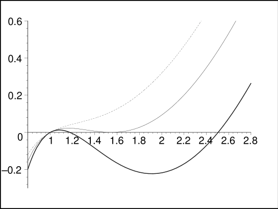
Figure 1: $F_{\mathrm{nut}}(r)$ versus $r$ with $\mathcal{B}=\mathbb{CP}^{2}$ for $N=1$, $\alpha=0.1$, $\Lambda=-2$, and $q=q_{\mathrm{crit}}=24.815$ (continuous line), $q<q_{\mathrm{crit}}$ (dotted line) and $q>q_{\mathrm{crit}}$ (bold line).

As in the case of solutions of Gauss-Bonnet gravity in the absence of electromagnetic field, the solution with base space ${\cal B}=S^{2}\times S^{2}$ does not satisfy the conditions of NUT solutions. Computation of the Kretschmann scalar at $r=N$ for the solutions in six dimensions shows that the spacetime with ${\cal B}=S^{2}\times S^{2}$ has a curvature singularity at $r=N$ in Einstein gravity, while the spacetime with ${\cal B}={\mathbb{C}P}^{2}$ has no curvature singularity at $r=N$. Thus, the conjecture given in Deh1 is confirmed even in the presence of electromagnetic field. Indeed, we have non-extreme NUT solutions in $6$ dimensions with non-trivial fibration when the $4$-dimensional base space is chosen to be ${\mathbb{C}P}^{2}$.

On the other hand, the solutions with ${\cal B}=T^{2}\times T^{2}={\cal B}_{A}$ and ${\cal B}=T^{2}\times S^{2}={\cal B}_{B}$ are extermal NUT solution provided the charge parameter is less than the critical value $q_{{\rm crit}}$ and the mass parameter is fixed to be

$$m_{n}^{A} = -\frac{16}{5}\Lambda N^{5}-\frac{3}{4}\frac{q^{2}}{N^{3}},$$ (20)

$$m_{n}^{B} = -\frac{8}{15}N^{3}(6\Lambda N^{2}+5)-\frac{3}{4}\frac{q^{2}}{N^{3}}$$ (21)

Indeed for these two cases $F^{\prime}(r=N)=0$, and therefore the NUT solutions should be regarded as extremal solutions. As in the case of non-extreme NUT solution, the critical value $q_{{\rm crit}}$ depends on $\alpha$, $\Lambda$ and $N$, and it is not easy to give an analytic expression for it. The critical value of $q$ for ${\cal B}_{A}=T^{2}\times T^{2}$ and ${\cal B}_{B}=T^{2}\times S^{2}$ may be found by solving the system of two equations (18). See Figs. 2 and 3 for more details.

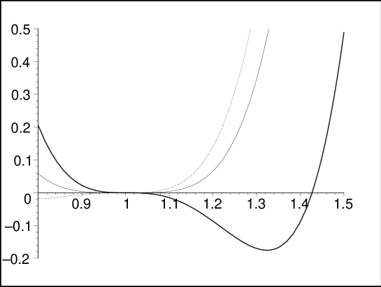
Figure 2: $F_{\mathrm{nut}}(r)$ versus $r$ with $\mathcal{B}_{B}=T^{2}\times T^{2}$ for $N=1$, $\alpha=0.1$, $\Lambda=-2$, and $q_{\mathrm{crit}}=11.322$ (continuous line), $q<q_{\mathrm{crit}}$ (dotted line) and $q>q_{\mathrm{crit}}$ (bold line).

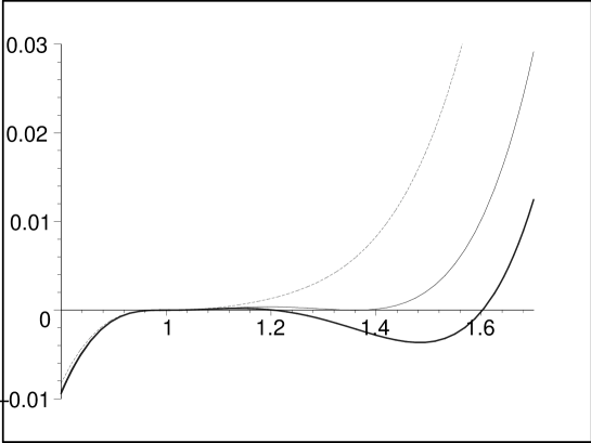
Figure 3: $F_{\mathrm{nut}}(r)$ versus $r$ with $\mathcal{B}_{B}=T^{2}\times S^{2}$ for $N=1$, $\alpha=0.1$, $\Lambda=-2$, and $q_{\mathrm{crit}}=19.973$ (continuous line), $q<q_{\mathrm{crit}}$ (dotted line) and $q>q_{\mathrm{crit}}$ (bold line).

Computing the Kretschmann scalar, we find that there is a curvature singularity at $r=N$  for the spacetime with ${\cal B}={\cal B}_{B}$, while the spacetime with ${\cal B}_{A}$ has no curvature singularity at $r=N$. Thus, the second conjecture of Ref. Deh1 can be extended to the case of Gauss-Bonnet gravity in the presence of electromagnetic field. Indeed, when the base space has at most one two dimensional curved space as one of its factor spaces, then Gauss-Bonnet-Maxwell gravity admits an extreme NUT solution even though there exists a curvature singularity at $r=N$. As in the case of uncharged solutions of Gauss-Bonnet gravity, the extreme NUT solution for the base space $T^{2}\times T^{2}$ in the absence of cosmological constant ($\Lambda=0$) has no horizon and the singularity is naked.

III.2 Taub-Bolt Solutions

The conditions for having a regular bolt solution are (i) $F(r=r_{b})=0$, (ii)$\ F^{\prime}(r_{b})=1/(3N)$ and (iii)

$$V\equiv V_{b}=-\frac{qr_{b}}{r_{b}^{4}-6N^{2}r_{b}^{2}-3N^{4}}$$ (22)

with $r_{b}>N$. Condition (ii), which again follows from the fact that we want to avoid a conical singularity at the bolt, together with the fact that the period of $\tau$ will still be $12\pi N$ and $V=V_{b}$, gives the following equation for $r_{b}$

$$3N\Lambda{r_{b}}^{4}+2{r_{b}}^{3}-6N(\Lambda N^{2}+1){r_{b}}^{2}-2(N^{2}-4\alpha)r_{b}+3\Lambda N^{5}+6N^{3}-\zeta\alpha N-27N(\frac{V_{b}}{r_{b}})^{2}(r_{b}^{2}-N^{2})^{2}=0$$

where $\zeta$ is $8$ and $12$ for the base spaces ${\mathbb{C}P}^{2}$ and $S^{2}\times S^{2}$ respectively.

Next we consider the Taub-bolt solutions for ${\cal B}=T^{2}\times S^{2}$ and ${\cal B}=T^{2}\times T^{2}$. Euclidean regularity at the bolt requires the period of $\tau$ to be

$$\beta=\frac{8\pi r_{b}^{3}(r_{b}^{2}-N^{2}+2\alpha)}{r_{b}^{2}(r_{b}^{2}-N^{2})[1-\Lambda(r_{b}^{2}-N^{2})]+9V_{b}^{2}(r_{b}^{2}-N^{2})^{2}}$$ (23)

for ${\cal B}=T^{2}\times S^{2}$, and

$$\beta=-\frac{8\pi r_{b}^{3}}{(r_{b}^{2}-N^{2})(\Lambda r_{b}^{2}-9V_{b}^{2})}$$ (24)

for ${\cal B}=T^{2}\times T^{2}$. As $r_{b}$ varies from $N$ to infinity, one covers the whole temperature range from $0$ to $\infty$, and therefore we have non-extreme bolt solutions. Indeed, the fibration in the latter case is trivial: there are no Misner strings. The boundary has trivial topology and therefore the Euclidean time period $\beta$ will not be fixed, as it was in the ${\cal B}={\mathbb{C}P}^{2}$ case, by the value of the NUT parameter Myers2 . Again, as in the case of uncharged solution Deh1 , there is no bolt solution with ${\cal B}=T^{2}\times T^{2}$ in the absence of cosmological constant.

IV Eight-dimensional Solutions

In eight dimensions there are more possibilities for the base space ${\cal B}$. It can be a $6$-dimensional space, a product of three $2$-dimensional spaces, or the product of a $4$-dimensional space with a $2$-dimensional one. We first consider the differential equation for vector potential (7). Equation (5) has the same form for any base space ${\cal B}$ as

$$(r^{2}-N^{2})^{2}h^{\prime\prime}(r)+6r(r^{2}-N^{2})h^{\prime}(r)-12N^{2}h(r)=0$$ (25)

with the solution

$$h(r)=\frac{1}{(r^{2}-N^{2})^{3}}\left[qr+V(r^{6}-5N^{2}r^{4}+15N^{4}r^{2}+5N^{6})\right]$$ (26)

where $V$ and $q$ are two arbitrary constants which correspond to electric potential at infinity  and electric charge respectively.

For any base space, the form of the function $F(r)$ is

$$F(r) = \frac{(r^{2}-N^{2})^{2}}{8\alpha(5r^{2}+3N^{2})}\left(1+\frac{4p\alpha}{3(r^{2}-N^{2})}-\sqrt{B(r)+C(r)}\right)$$

$$B(r) = 1-\frac{16\alpha mr\left(5r^{2}+3N^{2}\right)}{3(r^{2}-N^{2})^{5}}+\frac{16p\alpha N^{2}}{15(r^{2}-N^{2})^{5}}(r^{6}-15N^{2}r^{4}-45N^{4}r^{2}-5N^{6})$$ (27)

$$+\frac{16\alpha\Lambda\left(5r^{2}+3N^{2}\right)}{105(r^{2}-N^{2})^{5}}(5r^{8}-28N^{2}r^{6}+70N^{4}r^{4}-140N^{6}r^{2}-35N^{8})$$

$$+\frac{4\alpha\left(5r^{2}+3N^{2}\right)}{9N^{5}(r^{2}-N^{2})^{8}}\{12N^{5}(5r^{2}-N^{2})q^{2}-384N^{7}r^{3}(r^{2}-5N^{2})qV$$

$$+48N^{7}(r^{10}-25N^{2}r^{8}-70N^{4}r^{6}+350N^{6}r^{4}-75N^{8}r^{2}+75N^{10})V^{2}\}$$

where $p$ is again the dimension of the curved factor spaces of ${\cal B}$, and the function $C(r)$ depends on the choice of the base space. The function $C(r)$ for various base spaces are

${\cal B}$	$p$	$(r^{2}-N^{2})^{5}C(r)/\alpha^{2}$
${\,{{\mathbb{C}P}^{3}}}$	6	$-16(r^{6}-15N^{2}r^{4}-45N^{4}r^{2}-5N^{6})-20D(r)$
$S^{2}\times{\mathbb{C}P}^{2}$	6	$-\frac{64}{27}(13r^{6}-135N^{2}r^{4}-345N^{4}r^{2}-45N^{6})+60D(r)$
$S^{2}\times S^{2}\times S^{2}$	6	$-\frac{128}{3}(r^{6}-9N^{2}r^{4}-21N^{4}r^{2}-3N^{6})+20D(r)$
$T^{2}\times{\mathbb{C}P}^{2}$	4	$\frac{128}{27}(r^{6}+9N^{2}r^{4}+51N^{4}r^{2}+3N^{6})-60D(r)$
$T^{2}\times S^{2}\times S^{2}$	4	$-\frac{64}{9}(r^{6}-15N^{2}r^{4}-45N^{4}r^{2}-5N^{6})-60D(r)$
$T^{2}\times T^{2}\times S^{2}$	2	$\frac{64}{9}(r^{2}-N^{2})^{3}-20D(r)$
$T^{2}\times T^{2}\times T^{2}$	0	–$20D(r)$

where

$$D(r)=\frac{r(5r^{2}+3N^{2})}{9\alpha N^{5}}q^{2}$$ (28)

One may note that the asymptotic behavior of all of these solutions is locally AdS for $\Lambda<0$ provided $\left|\Lambda\right|<21/(80\alpha)$, locally dS for $\Lambda>0$ and locally flat for $\Lambda=0$. Note that all the different $F(r)$’s given in this section have the same form as $\alpha$ goes to zero. Also, one may note that these solutions reduce to the solutions of Gauss-Bonnet gravity Deh1 when $q$ and $V$ vanish.

IV.1 Taub-NUT Solutions

As in the case of six-dimensional spacetimes, the solutions given in Eq. (27) describe NUT solutions, if (i) $F(r=N)=0$, (ii) $F^{\prime}(r=N)=1/(4N)$, (iii) $h(r=N)=0$ and (iv) $q<q_{{\rm crit}}$, where $q_{{\rm crit}}$ is the solution of the system of two equations (18). Using the third conditions which comes from the regularity of vector potential at $r=N$  gives

$$V\equiv V_{n}=-\frac{q}{16N^{5}},$$ (29)

It is easy to show that Gauss-Bonnet-Maxwell gravity in eight dimensions admits non-extreme NUT solutions only when the base space is chosen to be ${\mathbb{C}P}^{3}$. The conditions for a nonsingular NUT solution are satisfied provided the mass parameter is fixed to be

$$m_{n}=-\frac{8N^{3}}{105}(16\Lambda N^{4}+42N^{2}-105\alpha)-\frac{5}{12}\frac{q^{2}}{N^{5}}$$ (30)

On the other hand, the solutions with ${\cal B}=T^{2}\times T^{2}\times T^{2}={\cal B}_{A}$ and ${\cal B}=T^{2}\times T^{2}\times S^{2}={\cal B}_{B}$ are extermal NUT solutions provided the mass parameter is

$$m_{n}^{A} = -\frac{128}{105}\Lambda N^{7}-\frac{5}{12}\frac{q^{2}}{N^{5}},$$ (31)

$$m_{n}^{B} = -\frac{16N^{5}}{105}(8\Lambda N^{2}+7)-\frac{5}{12}\frac{q^{2}}{N^{5}}$$ (32)

These results for eight-dimensional Gauss-Bonnet gravity are consistent with the conjectures of Ref. Deh1 . Again, one may note that the former extremal NUT solution does not have a curvature singularity at $r=N$ whereas the latter does.

IV.2 Taub-Bolt Solutions

The conditions for having a regular bolt solution are $F(r=r_{b})=0$, $F^{\prime}(r_{b})=1/(4N)$ and

$$V\equiv V_{b}=-\frac{qr_{b}}{r_{b}^{6}-5N^{2}r_{b}^{4}+15N^{4}r_{b}^{2}+5N^{6}}$$ (33)

with $r_{b}>N$. The second condition again follows from the fact that we want to avoid a conical singularity at the bolt, together with the fact that the period of $\tau$ will still be $16\pi N$. Now applying these conditions for the curved base spaces gives the following equation for $r_{b}$

$$4N\Lambda{r_{b}}^{4}+3{r_{b}}^{3}-4N(3+2\Lambda N^{2}){r_{b}}^{2}+3(8\alpha-N^{2})r_{b}+4N(\Lambda N^{4}+3N^{2}-\zeta\alpha)-100N(\frac{V_{b}}{r_{b}})^{2}(r_{b}^{2}-N^{2})^{2}=0$$

where $\zeta$ is $9$, $32/3$ and $12$ for the base spaces ${\mathbb{C}P}^{3}$, $S^{2}\times{\mathbb{C}P}^{2}$ and $S^{2}\times S^{2}\times S^{2}$ respectively.

For the case of ${\cal B}=T^{2}\times T^{2}\times T^{2}$ and ${\cal B}=T^{2}\times T^{2}\times S^{2}$, Euclidean regularity at the bolt requires the period of $\tau$ to be

$$\beta=-\frac{12\pi r_{b}^{3}}{({r_{b}}^{2}-N^{2})(\Lambda{r_{b}}^{2}-25V_{b}^{2})}$$ (34)

and

$$\beta=\frac{4\pi r_{b}^{3}(3{r_{b}}^{2}-3N^{2}+8\alpha)}{{r_{b}}^{2}({r_{b}}^{2}-N^{2})[1-\Lambda({r_{b}}^{2}-N^{2})]+25V_{b}^{2}({r_{b}}^{2}-N^{2})^{2}}$$ (35)

respectively. As $r_{b}$ varies from $N$ to infinity, one covers the whole temperature range from $0$ to $\infty$, and therefore one can have bolt solutions. Again, one may note that there is no asymptotic locally flat black hole solutions with base space ${\cal B}=T^{2}\times T^{2}\times T^{2}$.

V Ten-dimensional Solutions

In ten dimensions there are more possibilities for the base space ${\cal B}$. It can be an $8$-dimensional space, the product of a $6$-dimensional space with a $2$-dimensional one, a product of two $4$-dimensional spaces, a product of a $4$-dimensional space with two $2$-dimensional spaces, or the product of four $2$-dimensional spaces. Substituting the vector potential (7) in source free Maxwell equation (5), for a ten-dimensional spacetime of the form given in Eq. (6) with an arbitrary base space ${\cal B}$ , one obtains

$$(r^{2}-N^{2})^{2}h^{\prime\prime}(r)+8r(r^{2}-N^{2})h^{\prime}(r)-16N^{2}h(r)=0$$ (36)

with the solution

$$h(r)=\frac{1}{5(r^{2}-N^{2})^{4}}\{5qr+V(5r^{8}-28N^{2}r^{6}+70N^{4}r^{4}-140N^{6}r^{2}-35N^{8})\}$$ (37)

where $V$ and $q$ are two arbitrary constants which correspond to electric potential at infinity and electric charge respectively.

The form of the function $F(r)$ for any base space ${\cal B}$ may be written as

$$F(r) = \frac{(r^{2}-N^{2})^{2}}{12\alpha(7r^{2}+3N^{2})}\left(1+\frac{3p\alpha}{2(r^{2}-N^{2})}-\sqrt{B(r)+C(r)}\right),$$

$$B(r) = 1+\frac{36\alpha mr\left(7r^{2}+3N^{2}\right)}{(r^{2}-N^{2})^{6}}+\frac{6p\alpha N^{2}}{35(r^{2}-N^{2})^{6}}(3r^{8}-28N^{2}r^{6}+210N^{4}r^{4}+420N^{6}r^{2}+35N^{8})$$ (38)

$$+\frac{2\alpha\Lambda\left(7r^{2}+3N^{2}\right)}{21(r^{2}-N^{2})^{6}}(7r^{10}-45N^{2}r^{8}-126N^{4}r^{6}-210N^{6}r^{4}+315N^{8}r^{2}+63N^{10})$$

$$+\frac{3\alpha\left(7r^{2}+3N^{2}\right)}{32N^{7}(r^{2}-N^{2})^{10}}\{64N^{7}(7r^{2}-N^{2})q^{2}-4096N^{9}r^{3}(35N^{4}-14N^{2}r^{2}+3r^{4})qV+$$

$$1024N^{9}(5r^{14}-77N^{2}r^{12}+861N^{4}r^{10}-525N^{6}r^{8}-5145N^{8}r^{6}+11025N^{10}r^{4}$$

$$-1225N^{12}r^{2}+1225N^{14})V^{2}\}$$

where $p$ is the dimensionality of the curved portion of the base space, and the function $C(r)$ depends on the choice of the base space ${\cal B}$. The function $C(r)$ for different base spaces are listed in the following table

${\cal B}$	$p$	$(r^{2}-N^{2})^{6}C(r)/\alpha^{2}$
${{\mathbb{C}P}^{4}}$	8	$-\frac{144}{25}(3r^{8}-28N^{2}r^{6}+210N^{4}r^{4}+420N^{6}r^{2}+35N^{8})-21D(r)$
${\mathbb{C}P}^{2}\times{\mathbb{C}P}^{2}$	8	$-\frac{16}{5}(11r^{8}-76N^{2}r^{6}+450N^{4}r^{4}+820N^{6}r^{2}+75N^{8})-630D(r)$
$S^{2}\times{\mathbb{C}P}^{3}$	8	$-\frac{18}{5}(9r^{8}-64N^{2}r^{6}+390N^{4}r^{4}+720N^{6}r^{2}+65N^{8})+630D(r)$
$S^{2}\times S^{2}\times{\mathbb{C}P}^{2}$	8	$-\frac{8}{5}(29r^{8}-184N^{2}r^{6}+990N^{4}r^{4}+1720N^{6}r^{2}+165N^{8})-630D(r)$
$S^{2}\times S^{2}\times S^{2}\times S^{2}$	8	-$\frac{285}{5}(r^{8}-6N^{2}r^{6}+300N^{4}r^{4}+50N^{6}r^{2}+5N^{8})-630D(r)$
$T^{2}\times{\mathbb{C}P}^{3}$	6	$\frac{27}{5}(r^{8}+4N^{2}r^{6}-90N^{4}r^{4}-220N^{6}r^{2}-15N^{8})-630D(r)$
$T^{2}\times S^{2}\times{\mathbb{C}P}^{2}$	6	$-\frac{1}{5}(43r^{8}-428N^{2}r^{6}+3330N^{4}r^{4}+6740N^{6}r^{2}+555N^{8})-630D(r)$
$T^{2}\times S^{2}\times S^{2}\times S^{2}$	6	$-\frac{9}{5}(11r^{8}-76N^{2}r^{6}+450N^{4}r^{4}+820N^{6}r^{2}+75N^{8})-630D(r)$
$T^{2}\times T^{2}\times{\mathbb{C}P}^{2}$	4	$\frac{4}{5}(17r^{8}-52N^{2}r^{6}-90N^{4}r^{4}-500N^{6}r^{2}-15N^{8})-630D(r)$
$T^{2}\times T^{2}\times S^{2}\times S^{2}$	4	$\frac{12}{5}(r^{8}+4N^{2}r^{6}-90N^{4}r^{4}-220N^{6}r^{2}-15N^{8})-630D(r)$
$T^{2}\times T^{2}\times T^{2}\times S^{2}$	2	$9(r^{2}-N^{2})^{4}+105D(r)$
$T^{2}\times T^{2}\times T^{2}\times T^{2}$	0	$105D(r)$

where

$$D(r)=\frac{r(7r^{2}+3N^{2})}{32\alpha N^{7}}q^{2}$$ (39)

Note that the asymptotic behavior of all of these solutions is locally AdS for $\Lambda<0$ provided $\left|\Lambda\right|<9/(42\alpha)$, locally dS for $\Lambda>0$ and locally flat for $\Lambda=0$. As with the $6$ and $8$ dimensional cases, all the different $F(r)$’s have the same form as $\alpha$ goes to zero. Also, one may note that these solutions reduce to those given in Deh1 when $q$ and $V$ vanish.

V.1 Taub-NUT Solutions

In order to have NUT solutions, the four conditions (i) $F(r=N)=0$, (ii) $F^{\prime}(r=N)=1/(5N)$, (iii) the regularity of vector potential at $r=N$,

$$V\equiv V_{n}=\frac{5q}{128N^{7}},$$ (40)

and (iv) the restriction on $q<q_{{\rm crit}}$, where $q_{{\rm crit}}$ is the solution of the system of two equations (18) should be satisfied. Using these four condition, we find that Gauss-Bonnet gravity in ten dimensions admits non-extreme NUT solutions only when the base space is chosen to be ${\mathbb{C}P}^{4}$, provided the mass parameter is fixed to be

$$m_{n}=-\frac{128N^{5}}{4725}(25\Lambda N^{4}+90N^{2}-378\alpha)-\frac{35}{128}\frac{q^{2}}{N^{7}}$$ (41)

On the other hand, the solutions with ${\cal B}=T^{2}\times T^{2}\times T^{2}\times T^{2}={\cal B}_{A}$ and ${\cal B}=T^{2}\times T^{2}\times T^{2}\times S^{2}={\cal B}_{B}$ are extermal NUT solution provided the mass parameter is

$$m_{n}^{A} = -\frac{128}{189}\Lambda N^{9}-\frac{35}{128}\frac{q^{2}}{N^{7}},$$ (42)

$$m_{n}^{B} = -\frac{64N^{7}}{945}(10\Lambda N^{2}+9)-\frac{35}{128}\frac{q^{2}}{N^{7}}$$ (43)

and $q<q_{{\rm crit}}$. It is also straightforward to show that the former extremal NUT solution has no curvature singularity at $r=N$, whereas the latter has. These results in ten-dimensions shows that the conjectures of Ref. Deh1 may be extended to the case of Gauss-Bonnet-Maxwell gravity.

V.2 Taub-Bolt Solutions

Now applying the conditions for having a regular bolt solution $F(r=r_{b})=0$, $F^{\prime}(r_{b})=1/(5N)$ with $r_{b}>N$ and

$$V\equiv V_{b}=-\frac{5qr_{b}}{5r_{b}^{8}-28N^{2}r_{b}^{6}+70N^{4}r_{b}^{4}-140N^{6}r_{b}^{2}-35N^{8}}$$

for the curved base spaces gives the following equation for $r_{b}$

$$5N\Lambda{r_{b}}^{4}+4{r_{b}}^{3}-10N(2+\Lambda N^{2}){r_{b}}^{2}+4(12\alpha-N^{2})r_{b}$$

$$+N(5\Lambda N^{4}+20N^{2}-\zeta\alpha)-245N(\frac{V_{b}}{r_{b}})^{2}(r_{b}^{2}-N^{2})^{2}=0$$

where $\zeta$ is equal to 96, 105, 320/3, 340/3 and 120 for the base spaces ${\mathbb{C}P}^{4}$, $S^{2}\times{\mathbb{C}P}^{3}$, ${\mathbb{C}P}^{2}\times{\mathbb{C}P}^{2}$, $S^{2}\times S^{2}\times{\mathbb{C}P}^{2}$ and $S^{2}\times S^{2}\times S^{2}\times S^{2}$ respectively.

For the case of ${\cal B}=T^{2}\times T^{2}\times T^{2}\times T^{2}$ and ${\cal B}=S^{2}\times T^{2}\times T^{2}\times T^{2}$, Euclidean regularity at the bolt requires the period of $\tau$ to be

$$\beta=-\frac{16\pi r_{b}^{3}}{({r_{b}}^{2}-N^{2})(\Lambda{r_{b}}^{2}-49V_{b}^{2})}$$ (44)

and

$$\beta=\frac{16\pi r_{b}^{3}({r_{b}}^{2}-N^{2}+3\alpha)}{{r_{b}}^{2}({r_{b}}^{2}-N^{2})[1-\Lambda({r_{b}}^{2}-N^{2})]+49V_{b}^{2}({r_{b}}^{2}-N^{2})^{2}}$$ (45)

respectively. As $r_{b}$ varies from $N$ to infinity, one covers the whole temperature range from $0$ to $\infty$, and therefore one can have bolt solutions. Again, one may note that for the case of an asymptotic locally flat solution with base space ${\cal B}=T^{2}\times T^{2}\times T^{2}\times T^{2}$, there is no black hole solution.

VI The $(2k+2)$-dimensional Taub-NUT solutions

In this section we present the $(2k+2)$-dimensional solution of Gauss-Bonnet-Maxwell gravity. The electromagnetic field equation (5) for the metric (6) in $2k+2$ dimensions is

$$(r^{2}-N^{2})^{2}h^{\prime\prime}(r)+2kr(r^{2}-N^{2})h^{\prime}(r)-4kN^{2}h(r)=0$$ (46)

The solution of Eq. (46) may be expressed in terms of hypergeometric function ${}_{2}F_{1}([a,b],[c],z)$ in a compact form. The result is

$$h(r)=\frac{1}{(r^{2}-N^{2})^{k}}\left(qr-(-1)^{k}(2k-1)VN^{2k}\,_{2}F_{1}\left(\left[-\frac{1}{2},-k\right],\left[\frac{1}{2}\right],\frac{r^{2}}{N^{2}}\right)\right)$$ (47)

where $V$ and $q$ are two arbitrary constants which correspond to electric potential at infinity and charge respectively.

Here, we consider only those cases which Gauss-Bonnet-Maxwell gravity admits NUT solutions, leaving out the other cases which one has only bolt solution for reasons of economy. There are three cases which we have NUT solutions in $2k+2$ dimensions.

The only case which Gauss-Bonnet gravity admits non-extreme NUT solution in $2k+2$ dimensions is when the base space is ${\cal B}={\mathbb{C}P}^{k}$. To find the function $F(r)$, one may use any components of Eq. (4). The simplest equation is the $tt$ component of these equations which can be written as

$$\Omega_{1}rF^{\prime}(r)+\Omega_{2}F^{2}(r)+\Omega_{3}F(r)+\Omega_{4}=\left[h^{\prime\prime}(r)\right]^{2}+\frac{4kN^{2}}{(r^{2}-N^{2})^{2}}h^{2}(r),$$ (48)

where $h(r)$ is given in Eq. (47) and $\Omega_{1}$ to $\Omega_{4}$ are

$$\Omega_{1} = -\alpha\left((2k-1)r^{2}+3N^{2}\right)F(r)+(r^{2}-N^{2})\left(\alpha+\frac{r^{2}-N^{2}}{4(k-1)}\right),$$

$$\Omega_{2} = -\frac{\alpha}{2(r^{2}-N^{2})}\left\{(2k-1)(2k-3)r^{4}+2(2k-7)N^{2}r^{2}+3N^{4}\right\},$$

$$\Omega_{3} = -\frac{(r^{2}-N^{2})[(2k-1)r^{2}+N^{2}]}{4(k-1)}+\alpha\left((2k-3)r^{2}+N^{2}\right),$$

$$\Omega_{4} = (r^{2}-N^{2})\left\{\Lambda\frac{(r^{2}-N^{2})^{2}}{4k(k-1)}-\frac{(r^{2}-N^{2})}{4(k-1)}-\frac{k\alpha}{2(k+1)}\right\}$$ (49)

The solutions of Eq. (48) describe NUT solutions, if (i) $F(r=N)=0$, (ii) $F^{\prime}(r=N)=[(k+1)N]^{-1}$, (iii) $h(r=N)=0$ and (iv) the charge $q$ is less than a critical value $q_{{\rm crit}}$, where $q_{{\rm crit}}$ is the solution of the system of two equations (18). The first condition comes from the fact that all the extra dimensions should collapse to zero at the fixed point set of $\partial/\partial\tau$, the second one ensures that there is no conical singularity with a smoothly closed fiber at $r=N$, the third one comes from the regularity of vector potential at  $r=N$ and the fourth condition comes up since $r=N$ should be the event horizon.

Using these conditions, one finds that the solutions of the differential equation (48) with $\Omega_{i}$’s of Eqs. (49) yield a non-extreme NUT solution for any given (even) dimension $k\geq 2$ provided

$$V\equiv V_{n}=\frac{(-1)^{k}}{2\sqrt{\pi}N^{2k-1}}\frac{\Gamma(k-\frac{1}{2})}{\Gamma(k+1)}q,$$ (50)

the mass parameter $m$ is fixed to be

$$m_{n} = -\frac{(k-2)!2^{k-1}N^{2k-3}}{(k+1)(2k+1)!!}\{8(k+1)^{2}\Lambda N^{4}+4k(k+1)(2k+1)N^{2}$$ (51)

$$-4k(2k+1)(2k-1)(k-1)\alpha\}-\frac{4\Gamma(k+\frac{1}{2})}{\sqrt{\pi}k\Gamma(k+1)}N^{1-2k}q^{2}$$

and $q<q_{{\rm crit}}$. This solution has no curvature singularity at $r=N$.

Solutions of Eqs. (48) and (49) for $m\neq m_{n}$ in any dimension can be regarded as bolt solutions. The value of the bolt radius $r_{b}>N$ may be found from the regularity conditions (i) $F(r=r_{b})=0$ and $F^{\prime}(r_{b})=[(k+1)N]^{-1}$. Applying these for ${\cal B}={\mathbb{C}P}^{k}$ gives the following equation for $r_{b}$

$$4(k+1)\Lambda N{r_{b}}^{4}+4k{r_{b}}^{3}-4(k+1)N\left[k+2\Lambda N^{2}\right]{r_{b}}^{2}+4k\left[4(k-1)\alpha-N^{2}\right]r_{b}$$

$$+N\left[4(k+1)\Lambda N^{4}+4k(k+1)N^{2}-8(k-1)k^{2}\alpha\right]-4(k+1)(2k-1)^{2}N(\frac{V_{b}}{r_{b}})^{2}(r_{b}^{2}-N^{2})^{2}=0$$

where $V_{b}$ is the solution of $h(r_{b})=0$.

Next we consider the solutions with the base space ${\cal B}=T^{2}\times...\times T^{2}$. The field equation is given by (48), where now

$$\Omega_{1} = -\alpha\{(2k-1)r^{2}+3N^{2}\}F+\frac{(r^{2}-N^{2})^{2}}{4(k-1)},$$

$$\Omega_{2} = -\frac{\alpha}{2(r^{2}-N^{2})}\left\{(2k-1)(2k-3)r^{4}+2(2k-7)N^{2}r^{2}+3N^{4}\right\},$$

$$\Omega_{3} = -\frac{(r^{2}-N^{2})[(2k-1)r^{2}+N^{2}]}{4(k-1)},$$

$$\Omega_{4} = \Lambda\frac{(r^{2}-N^{2})^{3}}{4k(k-1)}$$ (52)

The solutions of Eqs. (48) and (52) yield an extreme NUT solution for any given even dimension provided $q<q_{{\rm crit}}$ and the mass parameter $m$ is fixed to be

$$m_{n}=-\frac{(k+1)(k-2)!2^{k+2}}{(2k+1)!!}\Lambda N^{2k+1}-\frac{4\Gamma(k+\frac{1}{2})}{\sqrt{\pi}k\Gamma(k+1)}N^{1-2k}q^{2}$$ (53)

where in this case the spacetime has no curvature singularity at $r=N$. Also one may find that the Euclidean regularity at the bolt requires the period of $\tau$ to be

$$\beta=-\frac{4k\pi r_{b}^{3}}{({r_{b}^{2}}-N^{2})(\Lambda{r_{b}^{2}-(2k-1)}^{2}V_{b}^{2})}$$ (54)

and can have any value from zero to infinity as $r_{b}$ varies from $N$ to infinity, and therefore one can have bolt solution.

Finally, we consider the solution when ${\cal B}=S^{2}\times T^{2}\times...\times T^{2}$. In this case the field has the same form as Eq. (48) with

$$\Omega_{1} = -\alpha\{(2k-1)r^{2}+3N^{2}\}F+(r^{2}-N^{2})\{\frac{\alpha}{k}+\frac{r^{2}-N^{2}}{4(k-1)}\},$$

$$\Omega_{2} = -\frac{\alpha}{2(r^{2}-N^{2})}\left\{(2k-1)(2k-3)r^{4}+2(2k-7)N^{2}r^{2}+3N^{4}\right\},$$

$$\Omega_{3} = -\frac{(r^{2}-N^{2})[(2k-1)r^{2}+N^{2}]}{4(k-1)}+\frac{4(k-1)}{k}\alpha\{(2k-3)r^{2}+N^{2}\},$$

$$\Omega_{4} = \frac{(r^{2}-N^{2})^{2}[\Lambda(r^{2}-N^{2})-1]}{4k(k-1)}$$ (55)

Solutions of Eqs. (48) with (55) yield a NUT solution for any given even dimension with curvature singularity at $r=N$, provided the mass parameter $m$ is fixed to be

$$m_{n}=-\frac{(k-2)!2^{k+1}}{(2k+1)!!}N^{2k-1}\left\{2(k+1)\Lambda N^{2}+(2k+1)\right\}-\frac{4\Gamma(k+\frac{1}{2})}{\sqrt{\pi}k\Gamma(k+1)}N^{1-2k}q^{2}$$ (56)

and $q<q_{{\rm crit}}$. Also one may find that the Euclidean regularity at the bolt requires the period of $\tau$ to be

$$\beta=\frac{4k\pi r_{b}^{3}({r_{b}}^{2}-N^{2}+\frac{4(k-1)}{k}\alpha)}{{r_{b}^{2}}({r_{b}^{2}}-N^{2})[1-\Lambda({r_{b}}^{2}-N^{2})]+{(2k-1)}^{2}V_{b}^{2}({r_{b}^{2}}-N^{2})^{2}}$$ (57)

Again, $\beta$ of Eq. (57) can have any value from zero to infinity as $r_{b}$ varies from $N$ to infinity, and therefore one can have bolt solution.

The asymptotic behavior of all of these solutions is locally AdS for $\Lambda<0$ provided $\left|\Lambda\right|<k(2k+1)/[(k-1)(2k-1)\alpha]$ locally dS for $\Lambda>0$ and locally flat for $\Lambda=0$ . All the different $F(r)$’s for differing base spaces have the same form as $\alpha$ goes to zero, while they reduce to the solutions of Gauss-Bonnet gravity constructed in Deh1 when $q=V=0$.

VII Concluding Remarks

We have presented a class of ($2k+2$)-dimensional Taub-NUT/bolt solutions in Gauss-Bonnet-Maxwell gravity with cosmological term. These solutions are constructed as $S^{1}$ fibrations over even dimensional spaces that in general are products of Einstein-Kähler spaces. We found that the function $F(r)$ of the metric depends on the specific form of the base factors on which one constructs the circle fibration, while the form of electromagnetic field is independent of the base space. This is different from the solution of the Einstein-Maxwell gravity where the metric in any dimension is independent of the specific form of the base factors. In the presence of electromagnetic field, there exist two extra parameters, in addition to the mass and the NUT charge, namely; the electric charge $q$ and the potential at infinity $V$.

We found that in order to have NUT charged black holes in Gauss-Bonnet-Maxwell gravity, in addition to the two conditions of uncharged NUT solutions, there exists two other conditions. The first extra condition comes from the regularity of vector potential at $r=N$ which gives a relation between $q$ and $V$. Indeed, the existence of the parameter $V$ enables us to get a regularity condition on the one-form potential which is identical to that required to obtain a NUT solution. If one of these parameters vanishes then the other one should be equal to zero and the solution reduces to the uncharged solution. The second extra condition comes from the fact that the horizon at $r=N$ should be the outer horizon of the black hole. Indeed, Gauss-Bonnet-Maxwell gravity admits NUT black holes provided the charge parameter is less than a critical value $q_{{\rm crit}}$, which may be obtained by solving the system of two equations (18). In any dimension, the mass parameter $m$ which is fixed by these four NUT conditions depends on the fundamental constant $\Lambda$, $\alpha$, $N$ and $q$.

We also found that when Gauss-Bonnet gravity admits non-extremal NUT solutions with no curvature singularity at $r=N$, then there exists a non-extremal NUT solution in Gauss-Bonnet-Maxwell gravity too. In $(2k+2)$-dimensional spacetime, this happens when the metric of the base space is chosen to be ${\mathbb{C}P}^{k}$. Indeed, Gauss-Bonnet-Maxwell gravity does not admit non-extreme NUT solutions with any other base space. We confirm that when the base space has at most a 2-dimensional curved factor space with positive curvature, then Gauss-Bonnet-Maxwell gravity admits extremal NUT solutions as in the case of uncharged solutions. Finally, we obtained the bolt solutions of Gauss-Bonnet-Maxwell gravity in various dimensions and different base spaces, and gave the equations which can be solved for the horizon radius of the bolt solution.

Although, we obtained the explicit form of the solutions in $6$, $8$ and $10$ dimensions, one can generalize these solutions in a similar manner for even dimensions higher than ten. We gave the vector potential and the differential equation of the function $F(r)$ in $2k+2$ dimensions. In ($2k+2$)-dimensional spacetime, we have only one non-extremal NUT solution with ${\mathbb{C}P}^{k}$ as the base space, and two extremal NUT solutions with the base spaces $T^{2}\times T^{2}\times.....\times T^{2}$ and $S^{2}\times T^{2}\times T^{2}\times.....\times T^{2}$. There is no curvature singularity for the first two case, while for the latter case, the spacetime has curvature singularity at $r=N$.

Insofar we see that the corrections of low energy limit of string theory single out a preferred base space in order to have NUT solutions. Thus, the investigation of the existence of NUT solutions in dimensionally continued gravity, or Lovelock gravity with higher order terms might provide us with a window on some interesting new corners of higher order gravity. Also, the study of thermodynamic properties of these solutions remains to be carried out in the future.

References

(1) M. B. Greens, J. H. Schwarz and E. Witten, Superstring
Theory, (Cambridge University Press, Cambridge, England, 1987); D. Lust and
S. Theusen, Lectures on String Theory, (Springer, Berlin, 1989); J.
Polchinski, String Theory, (Cambridge University Press, Cambridge,
England, 1998).
(2) B. Zwiebach, Phys. Lett. 156B, 315 (1985); B. Zumino,
Phys. Rep. 137, 109 (1986).
(3) D. Lovelock, J. Math. Phys. 12, 498 (1971); N. Deruelle
and L. Farina-Busto, Phys. Rev. D 41, 3696 (1990); G. A.
MenaMarugan, ibid. 46, 4320 (1992); ibid. 46, 4340 (1992).
(4) M. H. Dehghani and R. B. Mann, Phys. Rev. D 72, 124006
(2005).
(5) D. G. Boulware and S. Deser, Phys. Rev. Lett. 55, 2656
(1985); J. T. Wheeler, Nucl. Phys. B268, 737 (1986).
(6) D. L. Wiltshire, Phys. Lett. 169B, 36 (1986); Phys.
Rev. D 38, 2445 (1988).
(7) R. C. Myers and J. Z. Simon, Phys. Rev. D 38, 2434
(1988); R. C. Myers, Nucl. Phys. B289, 701 (1987).
(8) R. G. Cai, Phys. Rev. D 65, 084014 (2002).
(9) M. Cvetic, S. Nojiri and S. D. Odintsov, Nucl. Phys. B628, 295 (2002); S. Nojiri and S. D. Odintsov, Phys. Lett. 521B, 87
(2001).
(10) M. H. Dehghani, Phys. Rev. D 67, 064017 (2003); ibid. 69, 064024 (2004); ibid. 70, 064019 (2004).
(11) M. H. Dehghani and M. Shamirzaie, Phys. Rev. D 72,
124015 (2005).
(12) A. H. Taub, Annal. Math. 53, 472 (1951); E. Newman,
L. Tamburino and T. Unti, J. Math. Phys. 4, 915 (1963).
(13) F. A. Bais and P. Batenburg, Nucl. Phys. B253, 162
(1985).
(14) D. N. Page and C. N. Pope, Class. Quant. Grav. 4, 213
(1987).
(15) M. M. Akbar and G. W. Gibbons, Class. Quant. Grav. 20, 1787 (2003).
(16) M. M. Taylor-Robinson, hep-th/9809041.
(17) A. Awad and A. Chamblin, Class. Quant. Grav. 19, 2051
(2002).
(18) R. Clarkson, L. Fatibene and R. B. Mann, Nucl. Phys. B652, 348 (2003).
(19) R. B. Mann and C. Stelea, Class. Quant. Grav. 21,
2937 (2004).
(20) R. B. Mann and C. Stelea, hep-th/0508203.
(21) D. Astefanesei, R. B. Mann and E. Radu, Phys. Lett. 620B,1 (2005).
(22) D. Astefanesei, R. B. Mann and E. Radu, J. High Energy
Phys. 01, 049 (2005).
(23) D. R. Brill, Phys. Rev. D 133, B845 (1964).
(24) R. B. Mann and C. Stelea, Phys. Lett. 632B, 537
(2006).
(25) A. M. Awad, hep-th/0508235.
(26) E. Radu, Phys. Rev. D 67, 084030 (2003); Y. Brihaye,
E. Radu, Phys .Lett.615B, 1 (2005).
(27) C. V. Johnson and R. C. Myers, Phys. Rev. D 50, 6512
(1994); Phys. Rev. D 52, 2294 (1995).
(28) P. Hoxha, R. R. Martinez-Acosta, C. N. Pope, Class. Quant.
Grav. 17, 4207 (2000).
(29) A. Chamblin, R. Emparan, C. V. Johnson and R. C.
Myers, Phys. Rev. D 59, 064010 (1999).