DESY Theory Group
Notkestraße 85
22603 Hamburg
Germany

We study factorizations of topological string amplitudes on higher genus Riemann surfaces with multiple boundary components and find quantum ${\cal A}_{\infty}$-relations, which are the higher genus analog of the (classical) ${\cal A}_{\infty}$-relations on the disk. For topological strings with ${\hat{c}}=3$ the quantum ${\cal A}_{\infty}$-relations are trivially satisfied on a single D-brane, whereas in a multiple D-brane configuration they may be used to compute open higher genus amplitudes recursively from disk amplitudes. This can be helpful in open Gromov–Witten theory in order to determine open string higher genus instanton corrections.
Finally, we find that the quantum ${\cal A}_{\infty}$-structure cannot quite be recast into a quantum master equation on the open string moduli space.

Quantum ${\cal A}_{\infty}$-Structures
for Open-Closed Topological Strings

1 Introduction and summary

The perturbative topological closed string is by now quite well-studied. The holomorphic anomaly equations [1] suggest an interpretation of the topological string partition function as a wave function [2, 3], and current research is concentrating on understanding this wave function in terms of a non-perturbative completion of the topological string.

The open topological string is far from such an understanding — it is not even well-studied perturbatively. This work is a first step in this direction. We do not yet try to consider the analog of holomorphic anomalies for open strings; these are notoriously difficult to handle (cf. the remarks in [1]). Instead we concentrate on a more fundamental difference between open and closed topological strings.

Deformations of closed string moduli are not obstructed, i.e., they are not subject to some potential. This is reflected in the fact that the associated on-shell $L_{\infty}$ structure vanishes [4], which is the main reason for why $L_{\infty}$ structures played a minor rôle in the physical literature on topological closed strings.

The picture is quite different in open topological string theory (at tree-level). The open string moduli $s^{a}$ are obstructed because they are lifted by an effective superpotential [5],

$${\cal W}_{eff}=\sum_{m=1}^{\infty}\frac{1}{m}{\cal F}_{a_{1}\ldots a_{m}}s^{a_{1}}\ldots s^{a_{m}}$$

which is due to a non-vanishing on-shell ${\cal A}_{\infty}$ structure for the disk amplitudes ${\cal F}_{a_{1}\ldots a_{m}}$ [6]. Therefore, in contrast to closed topological strings homotopy algebras play a more important rôle in open topological string theory.

In [6] the ${\cal A}_{\infty}$-structure was derived from the bubbling of disks, which was induced by the insertion of the topological BRST operator. In the present work we extend this analysis to topological string amplitudes ${\cal F}^{g,b}_{A_{1}|\ldots|A_{b}}(t)$ on genus $g$ Riemann surfaces with $b$ boundary components. Here, $A_{i}$, for $i=1,\ldots,b$, is a collective index for the cyclically ordered topological observables, which are inserted at the $i^{th}$ boundary circle. $t$ is a closed string modulus. It turns out to be convenient to resume these amplitudes in the all-genus topological string amplitudes,

$${\cal F}^{b}_{A_{1}|\ldots|A_{b}}(g_{s},t)=\sum_{g=0}^{\infty}g_{s}^{2g+b-2}{\cal F}^{g,b}_{A_{1}|\ldots|A_{b}}(t)\ ,$$

where we introduced the topological string coupling constant $g_{s}$. The main result of this work then states that the all-genus topological string amplitudes ${\cal F}^{g,b}_{A_{1}|\ldots|A_{b}}(g_{s},t)$ satisfy the (cyclic) quantum ${\cal A}_{\infty}$-relations (1).

At first sight these relations look quite complicated, but they bear some interesting features:

1. There are no closed string factorization channels involved in these relations. This is essentially due to the fact that degenerations in the closed string channel correspond to (real) codimension $2$ boundaries of the moduli space of the Riemann surface, whereas the insertion of the BRST operator ’maps’ only to the (real) codimension $1$ boundary. This will be explained in detail in the present work. The quantum ${\cal A}_{\infty}$-structure is, therefore, simpler than the homotopy algebra structures that appear in Zwiebach’s open-closed string field theory [7, 4].

2. As it was pointed out in [8], in the context of the topological B-model, the (classical) ${\cal A}_{\infty}$-relations are trivially satisfied on a single D-brane. We find that this is true for the full quantum ${\cal A}_{\infty}$-relations in models with central charge $\hat{c}=3$. This fact relies on arguments involving the $U(1)$ R-charge of the topological observables.

3. On the other hand, in a situation with multiple D-branes the quantum ${\cal A}_{\infty}$-relations give rise to a sequence of linear systems for the amplitudes ${\cal F}^{g,b}_{A_{1}|\ldots|A_{b}}(t)$, which can be solved recursively starting from disk amplitudes. As an example, we find solutions to the linear system in the context of open string instanton counting on the elliptic curve in the companion paper [9].

For the derivation of the quantum ${\cal A}_{\infty}$-relations we make the technical assumption that every boundary component of the Riemann surface carries at least one observable. This is important, for otherwise there appear non-stable configurations, which correspond to non-compact directions in the moduli space of the Riemann surface. More specifically, these come from closed string factorization channels where a ’bare’ boundary component, i.e., without operator insertions, bubbles off from the rest of the Riemann surface. The appearance of a non-stable configuration indicates ambiguities in view of divergences of topological string amplitudes (cf. [9]).

As it is familiar from string field theory [7, 10] and recently from open topological string theory [11], homotopy algebras have a dual description in terms of a master equation on a dual supermanifold (in the present context, the open string moduli space). We briefly comment on this relation and find that we have to formally include the non-stable configurations, that we just alluded to, in order to recast the quantum ${\cal A}_{\infty}$-structure into the modified quantum master equation (43). We want to stress that on the way of deriving this relation some information on the topological string amplitudes is lost so that the quantum ${\cal A}_{\infty}$-structure is not faithfully mapped to the modified quantum master equation.

Before giving an outline of the paper we list some concrete models where the quantum ${\cal A}_{\infty}$-relations may be applied. (i) Consider the topological $B$-model on a Calabi–Yau $3$-fold ${\cal M}$ in the presence of $B$-type boundary conditions. The latter correspond to holomorphic vector bundles over holomorphic submanifolds or, more generally, to objects in the derived category of coherent sheaves on ${\cal M}$ [12, 13]. At the classical level the ${\cal A}_{\infty}$-structure was computed for some explicit D-brane configurations on non-compact Calabi–Yau manifolds in [8]. (ii) The mirror dual of such a model is the topological $A$-model on ${\cal M}$ with $A$-type boundary conditions describing Lagrangian submanifolds and the coisotropic D-branes of [14, 15]. These are objects in Fukaya’s ${\cal A}_{\infty}$ category [16]. Correlation functions in the $A$-model receive world-sheet instanton corrections, thus relating it to enumerative geometry of rational curves in ${\cal M}$ or holomorphic disks spanned between Lagrangian submanifolds. In this context the quantum ${\cal A}_{\infty}$-relations could provide a means of recursively computing higher genus open Gromov–Witten invariants from disk invariants. (iii) A last example are topologically twisted Landau–Ginzburg (LG) orbifolds with $B$-type boundary conditions. The D-branes correspond to equivariant matrix factorizations of the LG superpotential [17, 18].

The paper is organized as follows: In section 2 open-closed topological string amplitudes are defined, and basic symmetry properties as well as selection rules are reviewed. The main result, the quantum ${\cal A}_{\infty}$-relations for the amplitudes ${\cal F}^{b}_{A_{1}|\ldots|A_{b}}(g_{s},t)$, is stated and proven in section 3. We proceed with the discussion of some features of our result in section 4 and close with the derivation of the modified quantum master equation on the open string moduli space in section 5.

2 Open-closed topological string amplitudes

Let us start with reviewing the general setup of open-closed topological string theory. This will give us also some room to introduce notations. By definition a topological string theory is a 2d topological conformal field theory (TCFT) coupled to gravity.

So let us have a look at the TCFT first. The most important relation in the topological operator algebra [19] can be stated as the fact that the stress-energy tensor $T_{zz}$ is BRST exact, i.e.,

$$T_{zz}(z)=[Q,G_{zz}(z)]\ .$$ (1)

Here, $Q$ is the BRST operator and $G_{zz}$ is the fermionic current of the operator algebra. The $U(1)$ R-current $J_{z}(z)$ does not interest us for the moment, but will play an important role in subsequent sections.

Since we want to consider models on general oriented, bordered Riemann surfaces $\Sigma$ we have to specify boundary conditions on the currents. The only choice for picking these boundary conditions comes from the $U(1)$ automorphism of the topological operator algebra, which acts as a phase factor $e^{i\pi\varphi}$ on the fermionic currents $Q(z)$ and $G_{zz}(z)$. However, a single-valued correlation function requires that the difference of the phases between two boundary conditions is integral, $\Delta\varphi\in\mathbb{Z}$ (cf. [20] in the context of superconformal algebras). The overall phase is unphysical and can be set to zero, so that the currents of the topological operator algebra satisfy the simple relations

$${}\begin{array}[]{l@{~=~}l}W^{bos}\hfil~{}=~{}&{\bar{W}}^{bos}\\ W^{ferm}\hfil~{}=~{}&(-)^{s}{\bar{W}}^{ferm}\end{array}\quad\textrm{on}\quad\partial\Sigma\ ,$$

for integral $s$.

The observables of an open-closed string theory are the cohomology classes of the BRST operator $Q$. Bulk observables $\phi_{i}$ are in one-to-one correspondence with states in the closed string Hilbert space ${\cal H}_{cl}$, in short we write $\phi_{i}\in{\cal H}_{cl}$. Whereas boundary observables $\psi^{\alpha\beta}_{a}$ correspond to a states in the open string Hilbert space ${\cal H}^{\alpha\beta}_{op}$. The upper indices denote the boundary conditions, i.e., the topological D-branes, on either side of the field. The cyclical order of the boundary fields ensures that the boundary labels $\alpha,\beta,\ldots$, once determined, always match, so that we restrain ourselves from writing the boundary labels explicitly in the following. In a topological conformal field theory it is important to choose a particular representative of the BRST cohomology class by requiring [19]

$$[G_{0},\phi_{i}]=[{\bar{G}}_{0},\phi_{i}]=[(G_{0}+(-)^{s}{\bar{G}}_{0}),\psi^{\alpha\beta}_{a}]=0\ ,$$ (2)

which implies that the topological observables have conformal weight zero.

In view of relation (1) we can define topological descendents [21] associated with bulk and boundary observables: the bulk $2$-form descendent $\phi^{(2)}_{i}$ and the boundary $1$-form descendent $\psi^{(1)}_{a}$ are particularly important for us and satisfy the relations

$$[Q,\phi^{(2)}_{i}]=d\phi^{(1)}_{i}\quad\textrm{resp.}\quad[Q,\psi^{(1)}_{a}]=d\psi_{a}\ .$$ (3)

The coupling of the TCFT to 2d gravity is similar to the bosonic string and we can inherit the procedure to define amplitudes on bordered higher genus Riemann surfaces. For that we introduce the quantities

$$G_{m_{i}}:=\int_{\Sigma}d^{2}z~{}(G_{zz}\mu_{i}^{z}{}_{\bar{z}}+G_{{\bar{z}}{\bar{z}}}\mu_{i}^{\bar{z}}{}_{z})\ ,$$ (4)

which we have to insert in the path integral to account for zero modes related to the complex structure moduli space of the Riemann surface $\Sigma$. In (4) $\mu_{i}^{z}{}_{\bar{z}}$ denotes the Beltrami differential,

$$\mu_{i}^{z}{}_{\bar{z}}:=\frac{1}{2}g^{z{\bar{z}}}\frac{\partial}{\partial{m_{i}}}g_{{\bar{z}}{\bar{z}}}\ ,$$

corresponding to the complex structure modulus $m_{i}$. Using (1) and the definition of the stress-energy tensor, we deduce the relation

$$\bigl{\langle}\ldots[Q,G_{m_{i}}]\ldots\bigr{\rangle}=\frac{\partial}{\partial{m_{i}}}\bigl{\langle}\ldots\bigr{\rangle}\ .$$ (5)

2.1 Definition of the amplitudes

Having set up the basics we can start defining the topological string amplitude on oriented Riemann surfaces $\Sigma_{g,b}$ of genus $g$ with $b$ boundary components.

A measure on the moduli space of punctured bordered Riemann surfaces is defined consistently only for stable configurations, that is, if

$$2g+b-2+2n+\sum_{i=1}^{b}m_{i}\geq 0\ ,$$ (6)

where $n$ is the number of bulk observables and $m_{i}$ is the number of boundary observables inserted on the $i^{th}$ boundary component.

Riemann surfaces with Euler character $\chi_{g,b}=2-2g-b\leq-1$ do not possess conformal Killing vector fields, so that we are not forced to gauge the corresponding symmetry. Following the prescription in bosonic string theory the amplitudes are defined as

$${\cal F}^{g,b}_{A_{1}|\ldots|A_{b}}(t):=\int d^{3|\chi_{g,b}|}m~{}\bigl{\langle}P\!\!\int\!\!\psi_{a[1]_{1}}^{(1)}\ldots\int\!\!\psi_{a[1]_{m_{1}}}^{(1)}\big{|}\!\int\!\!\psi_{a[2]_{1}}^{(1)}\ldots\big{|}\ldots\big{|}e^{t^{i}\int\phi^{(2)}_{i}}\prod_{i=1}^{3|\chi_{g,b}|}G_{m_{i}}\bigr{\rangle}_{\Sigma_{g,b}}\ ,$$ (7)

where we introduced the collective index $A_{i}=a[i]_{1}\ldots a[i]_{m_{i}}$. $P$ means that the boundary descendents are integrated in cyclical order; subsequently we will refrain from writing $P$ explicitly. The integration over the complex structure moduli space of the punctured Riemann surface will be defined more carefully later in section 3.1.

The amplitudes (7) can be understood as generating function for all amplitudes with arbitrary number of bulk insertions. We will sometimes refer to the amplitudes (7) as deformed amplitudes as compared to undeformed ones where the closed string moduli $t^{i}$ are turn off, i.e., $t^{i}=0$. As already emphasized in [6] it is not possible to subsume the boundary observables as deformations because of the boundary condition labels and the cyclic ordering.

There are four Riemann surfaces which do have conformal Killing vectors and need special treatment. Let us start with the simplest one, the Riemann sphere $\Sigma_{0,0}=S^{2}$. The global conformal group is $SL(2,\mathbb{C})$, which can be gauged by fixing three bulk observables. The sphere three-point function defines the prepotential ${\cal F}={\cal F}^{0,0}$ in the well-known way:

$$\partial_{i}\partial_{j}\partial_{k}{\cal F}^{0,0}(t):=\bigl{\langle}\phi_{i}~{}\phi_{j}~{}\phi_{k}~{}e^{t^{i}\int\phi^{(2)}_{i}}\bigr{\rangle}_{\Sigma_{0,0}}\ .$$ (8)

On the torus $\Sigma_{1,0}$ the conformal Killing vectors correspond to translations and the complex structure moduli space ${\cal M}_{1,0}$ is the upper half complex plane mod $PSL(2,\mathbb{Z})$. The amplitude reads:

$$\partial_{i}{\cal F}^{1,0}(t):=\int d\tau d\bar{\tau}\bigl{\langle}\phi_{i}~{}e^{t^{i}\int\phi^{(2)}_{i}}~{}G_{\tau}~{}G_{\bar{\tau}}\bigr{\rangle}_{\Sigma_{1,0}}\ .$$ (9)

For the bordered Riemann surfaces with conformal Killing vectors the situation is a bit more complex for the reason that we can use either bulk or boundary observables to fix the global conformal symmetries. On the disk $\Sigma_{0,1}$ we need to fix three real positions, so that we can have two types of amplitudes (which are, however, related by Ward identities [6]):

$${\cal F}^{0,1}_{a_{1}\ldots a_{m}}(t):=-(-1)^{\tilde{a}_{2}+\ldots+\tilde{a}_{m-1}}\bigl{\langle}\psi_{a_{1}}\psi_{a_{2}}P\int\psi_{a_{3}}^{(1)}\ldots\int\psi_{a_{m-1}}^{(1)}\psi_{a_{m}}~{}e^{t^{i}\int\phi^{(2)}_{i}}\bigr{\rangle}_{\Sigma_{0,1}}\ ,$$ (10)

for $m\geq 3$, and

$$\partial_{i}{\cal F}^{0,1}_{a}(t):=\bigl{\langle}\phi_{i}\psi_{a}~{}e^{t^{i}\int\phi^{(2)}_{i}}\bigr{\rangle}_{\Sigma_{0,1}}\ ,$$ (11)

$$\partial_{i}{\cal F}^{0,1}_{ab}(t):=\bigl{\langle}\phi_{i}\psi_{a}\int\psi_{b}^{(1)}~{}e^{t^{i}\int\phi^{(2)}_{i}}\bigr{\rangle}_{\Sigma_{0,1}}{}\ .$$

On the annulus $\Sigma_{0,2}$ the rotation symmetry can be fixed by a boundary observable or a bulk descendent $\phi^{(1)}_{i}$ integrated along a contour from one boundary to the other, resulting in:

$${\cal F}^{0,2}_{A_{1}|A_{2}}(t):=\int_{0}^{\infty}dL\bigl{\langle}\psi_{a[1]_{1}}\!\!\int\!\!\psi_{a[1]_{2}}^{(1)}\ldots\!\!\int\!\!\psi_{a[1]_{m_{1}}}^{(1)}\big{|}\!\!\int\!\!\psi_{a[2]_{1}}^{(1)}\ldots\!\!\int\!\!\psi_{a[2]_{m_{2}}}^{(1)}\big{|}~{}e^{t^{i}\int\phi^{(2)}_{i}}G_{L}\bigr{\rangle}_{\Sigma_{0,2}}\ ,$$ (12)

for $m_{1}\geq 1$. For annulus amplitudes without any boundary insertions (cf. [1]) we define:

$$\partial_{i}{\cal F}^{0,2}_{.|.}(t):=\int_{0}^{\infty}dL\bigl{\langle}\int_{\cal C}\phi_{i}^{(1)}~{}e^{t^{i}\int\phi^{(2)}_{i}}~{}G_{L}\bigr{\rangle}_{\Sigma_{0,2}}\ ,$$ (13)

where the contour ${\cal C}$ runs from one boundary component to the other. The integration to ${\cal F}^{g,b}_{\ldots}$ in (8), (9) as well as (11), (13) is well-defined through conformal Ward identities [19, 6]. In the following we will assume that the integration constants in (11) are zero, i.e., ${\cal F}^{0,1}_{a}\big{|}_{t=0}={\cal F}^{0,1}_{ab}\big{|}_{t=0}=0$.

For later convenience we introduce the all-genus topological string amplitudes

$${\cal F}^{b}_{A_{1}|\ldots|A_{b}}(g_{s};t):=\sum_{g=0}^{\infty}g_{s}^{2g+b-2}~{}{\cal F}^{g,b}_{A_{1}|\ldots|A_{b}}(t){\qquad\mathrm{for}\quad}b\geq 1\ .$$ (14)

Note that for $b=0$ the analogous definition gives the topological closed string free energy ${\cal F}(g_{s};t)=\sum_{g=0}^{\infty}g_{s}^{2g-2}~{}{\cal F}^{g,0}(t)$ [1].

2.2 Topological twist and charge selection rules

Suppose we started with an ${\cal N}=(2,2)$ superconformal algebra (broken by boundary conditions to ${\cal N}=2$), which is part of a superstring compactification. We will leave the central charge $c=3{\hat{c}}$ arbitrary for the moment. The topological twist by $T\rightarrow T+\frac{1}{2}\partial J$ to the associated topological algebra is implemented by coupling the spin connection $\omega=\partial\ln(\sqrt{g})$ to the $U(1)$ current $J$ in the action [21, 23, 1], i.e.,

$$\frac{1}{8\pi}\int_{\Sigma_{g,b}}d^{2}z(\omega{\bar{J}}+\bar{\omega}J)\ .$$

Using the bosonization $J=i\sqrt{{\hat{c}}}\partial H$ and taking into account that we have boundaries we get

$$-\frac{i\sqrt{{\hat{c}}}}{8\pi}\int_{\Sigma_{g,b}}d^{2}z\sqrt{g}R^{(2)}H+c.c.-\frac{i\sqrt{{\hat{c}}}}{4\pi}\int_{\partial\Sigma_{g,b}}d\tau kH+c.c.\ ,$$ (15)

where $R^{(2)}$ is the world sheet curvature and $k$ is the geodesic curvature along the boundary. If we deform the world sheet metric such that the curvature localizes at $|\chi_{g,b}|$ points the twisting term (15) gives rise to $\chi_{g,b}$ insertions of the spectral flow operator $e^{-\frac{i}{2}\sqrt{{\hat{c}}}(H-{\bar{H}})}$ in the superconformal correlator, which, in total, carry the background $U(1)$ charge $-{\hat{c}}\chi_{g,b}$.

In view of these considerations the $U(1)$ charges $Q_{\alpha}$ of all operator insertions have to satisfy the condition

$$\sum_{\alpha=1}^{\#_{insert}}Q_{\alpha}={\hat{c}}\chi_{g,b}\ .$$

Let us consider an arbitrary Riemann surface $\Sigma_{g,b}$ with $\chi_{g,b}<0$. From the discussion in the previous section we know that we have to insert $-3\chi_{g,b}$ Beltrami differentials coupled to $G_{zz}$, which have charge $Q_{G}=-1$. Furthermore, every bulk descendent $\phi^{(2)}_{i}$ carries $Q_{i}=q_{i}-2$, where $q_{i}$ is the charge of the associated topological observable $\phi_{i}$, and every boundary descendent $\psi^{(1)}_{a}$ carries charge $Q_{a}=q_{a}-1$. The charge selection rule becomes

$$\sum_{i=1}^{n}q_{i}+\sum_{l=1}^{b}\sum_{a_{l}=1}^{m_{l}}q_{a_{l}}=2n+m+({\hat{c}}-3)\chi_{g,b}\ ,$$ (16)

where $n$ and $m=\sum_{l=1}^{b}m_{i}$ are the total number of bulk resp. boundary observables. Performing a case-by-case study it is easy to show that this formula extends to Riemann surfaces with $\chi_{g,b}\geq 0$, i.e., the sphere, the disk, the annulus and the torus.

2.3 Background fermion number - (suspended) $\mathbb{Z}_{2}$-grading

The bulk as well as the boundary fields of a general topological string theory carry a $\mathbb{Z}_{2}$-grading associated to the fermion number $F$. Just as for the $U(1)$ charge we have to cancel a background fermion number $\omega\in\mathbb{Z}_{2}$, which accounts for the insertion of fermionic zero modes in the path integral on the disk. In the context of matrix factorizations in Landau–Ginzburg models this is manifest in the Kapustin–Li formula [24, 25], whereas in the topological A- and B-model the background charge can be read off from the inner product for the Chern–Simons resp. holomorphic Chern–Simons action [26].

A generalization of the $\mathbb{Z}_{2}$-selection rule to arbitrary Riemann surfaces can readily be seen from a factorization argument within 2d topological field theory [27, 28]; every boundary component contributes $\omega$ to the background fermion number once, so that we obtain

$$\sum_{\alpha=1}^{\#_{insert}}F_{\alpha}=b~{}\omega\ .$$

Taking into account that the current $G_{zz}$ is odd we find $\sum_{i=1}^{n}F_{i}+\sum_{a=1}^{m}F_{a}=m+(\omega+1)b$ for the topological string amplitudes, where $F_{i}$ and $F_{a}$ are the fermion numbers for bulk resp. boundary observables.

Most of the subsequent formulas are conveniently expressed through the introduction of a suspended grading, which we define by:

$$\begin{array}[]{c@{~:=~}ll}\tilde{i}\hfil~{}:=~{}&F_{i}&\quad\textrm{for a bulk field}~{}\phi_{i}\ ,\\ \tilde{a}\hfil~{}:=~{}&F_{a}+1&\quad\textrm{for a boundary field}~{}\psi_{a}\ ,\end{array}$$ (17)

and $\tilde{\omega}:=\omega+1$. In other words, the suspended grading is the fermion number of the topological descendent rather than the topological observable itself. From now on we will refer to the notions even and odd with respect to the suspended grading. The $\mathbb{Z}_{2}$-selection rule takes the simple form

$$\sum_{i=1}^{n}\tilde{i}+\sum_{l=1}^{b}\sum_{a_{l}=1}^{m_{l}}\tilde{a}_{l}=b~{}\tilde{\omega}\ .$$ (18)

For most interesting models there is a close relation between the $\mathbb{Z}_{2}$-grading and the $U(1)$ charge. For Calabi–Yau compactifications this is simple, since the $U(1)$ charge is the form degree and the fermion number is the form degree mod $2$. In Gepner models, on the other hand, a relation is ensured in view of the orbifold action [29]. In particular, we have $({\hat{c}}-3)$ mod $2=\tilde{\omega}$.

Remark: For the rest of the paper we consider the case $\tilde{\omega}=0$, so that the $\mathbb{Z}_{2}$-selection rule is the same for arbitrary numbers of boundaries $b$, i.e.,

$$\sum_{i=1}^{n}\tilde{i}+\sum_{l=1}^{b}\sum_{a_{l}=1}^{m_{l}}\tilde{a}_{l}=0\ .$$

In many practical situations we can concentrate on even bulk fields. For instance, in Landau–Ginzburg models (not orbifolded!) the bulk chiral ring includes only even fields. In the topological $A$- and $B$-model the interest lies mainly on the marginal bulk operators, which are always even. Therefore, we subsequently consider only even bulk fields.

2.4 Symmetries, cyclic invariance, and unitality

In view of the topological nature of the amplitudes (14), we can deform the Riemann surface and exchange two boundary components. This leads to the graded symmetry:

$${\cal F}^{b}_{A_{1}|\ldots|A_{i}|A_{i+1}|\ldots|A_{b}}=(-)^{\tilde{A}_{i}\tilde{A}_{i+1}}{\cal F}^{b}_{A_{1}|\ldots|A_{i+1}|A_{i}|\ldots|A_{b}}{\qquad\mathrm{for}\quad}\forall~{}i=1,\ldots,b-1\ ,$$ (19)

where $\tilde{A}_{i}=\tilde{a}[i]_{1}+\ldots+\tilde{a}[i]_{m_{i}}$.

Moreover, the invariance of disk amplitudes under cyclic exchange of boundary observables naturally extends to $b\geq 1$, i.e.,

$${\cal F}^{b}_{A_{1}|\ldots|a[i]_{1}a[i]_{2}\ldots a[i]_{m_{i}}|\ldots|A_{b}}=(-)^{\tilde{a}[i]_{1}(\tilde{a}[i]_{2}+\ldots+\tilde{a}[i]_{m_{i}})}{\cal F}^{b}_{A_{1}|\ldots|a[i]_{2}\ldots a[i]_{m_{i}}a[i]_{1}|\ldots|A_{b}}\ .$$ (20)

The behavior of the topological amplitudes under insertion of the boundary unit operator ${1\!\!\!\!1\,}$ was investigated in [6] and it was shown that all tree-level amplitudes ${\cal F}^{0,1}_{a_{1}\ldots a_{m}}$ with at least one unit operator insertion vanish except for $m=3$. For all other amplitudes with $2g+b-2\geq 0$ it is easy to see that they vanish upon insertion of the unit, because the descendent of the unit vanishes, i.e., ${1\!\!\!\!1\,}^{(1)}=0$. We define unitality for the all-genus amplitudes ${\cal F}^{b}_{A_{1}|\ldots|A_{b}}$ as the properties:

$$\begin{array}[]{ll}{\cal F}^{1}_{{1\!\!\!\!1\,}ab}=(-)^{\tilde{a}}\rho_{ab}\\[10.0pt] {\cal F}^{b}_{a[1]_{1}\ldots{1\!\!\!\!1\,}\ldots a[1]_{m_{1}}|\ldots|A_{b}}=0&\textrm{otherwise}\ ,\end{array}$$ (21)

where

$$\rho_{ab}=\bigl{\langle}~{}{1\!\!\!\!1\,}~{}\psi_{a}\psi_{b}\bigr{\rangle}_{\Sigma_{0,1}}$$ (22)

is the topological open string metric. Note that the charge selection rule (16) for $\rho_{ab}$ reads $\tilde{a}+\tilde{b}=1$ (recall $\tilde{\omega}=0$), and the metric is (graded) symmetric

$$\rho_{ab}=(-)^{\tilde{a}\tilde{b}}\rho_{ba}\ .$$

Subsequently, we will use the topological open string metric $\rho_{ab}$ rather than the symplectic structure $\omega_{ab}=(-)^{\tilde{a}}\rho_{ab}$, which is commonly used in the literature on cyclic ${\cal A}_{\infty}$-structures [30, 10].

2.5 Special background charge ${\hat{c}}=3$

Topological string theories, for which the background charge ${\hat{c}}$ is equal to the critical dimension of the internal space of a superstring compactification, i.e., ${\hat{c}}=3$, have in many respects special properties. The topological closed string at tree-level is then governed by special geometry and the $tt^{*}$ equations; and through the ’decoupling’ of marginal operators from the relevant and irrelevant ones the holomorphic anomaly equations of [1] take a particularly simple form.

In our situation ${\hat{c}}=3$ is special in that the charge selection rule (16) is equal for arbitrary genus $g$ and number of boundaries $b$, which leads to similar conclusions as for the topological closed string [1]. First of all, an all-genus amplitude ${\cal F}^{b}_{a_{1}\ldots a_{m}}(g_{s};t)$, in which the fields satisfy the selection rule (16), gets contributions from all genera. This is not the case when ${\hat{c}}\neq 3$, because then ${\cal F}^{g,b}_{a_{1}\ldots a_{m}}$ is non-vanishing for at most one particular genus $\hat{g}$, i.e.,

$${}\begin{array}[]{r@{~=~}ll}{\cal F}^{b}_{A_{1}|\ldots|A_{b}}~{}=~{}&\sum_{g=0}^{\infty}g_{s}^{2g+b-2}{\cal F}^{g,b}_{A_{1}|\ldots|A_{b}}&{\qquad\mathrm{for}\quad}{\hat{c}}=3,\\[5.0pt] {\cal F}^{b}_{A_{1}|\ldots|A_{b}}~{}=~{}&g_{s}^{2{\hat{g}}+b-2}{\cal F}^{{\hat{g}},b}_{A_{1}|\ldots|A_{b}}&{\qquad\mathrm{for}\quad}{\hat{c}}\neq 3,~{}\textrm{and appr. genus}~{}{\hat{g}},\end{array}$$

where ${\hat{g}}$ is determined by $\tilde{A}_{1},\ldots,\tilde{A}_{b}$ and $b$ through the charge selection rule (16).

In fact, in many theories with ${\hat{c}}\neq 3$ there is no solution to the charge selection rule for ${\hat{g}}\geq 1$ at all. For example, in a topological string theory with ${\hat{c}}=1$, such as the topologically twisted non-linear sigma model on the torus or the associated Landau–Ginzburg orbifold, the boundary observables have charges in the range $0\leq q\leq 1$. Therefore, only Riemann surfaces with $\chi_{g,b}\geq 0$ give non-vanishing amplitudes. In particular, the annulus and the torus amplitudes admit only marginal operator insertions.

3 Quantum ${\cal A}_{\infty}$-category

As was shown in [6] the topological open string amplitudes satisfy a unital, cyclic ${\cal A}_{\infty}$-algebra at tree-level:

$$\sum_{l\leq k=1}^{m}(-)^{s_{l}}~{}{\cal F}^{0,1}_{a_{1}\ldots a_{l}ca_{k+1}\ldots a_{m}}\rho^{cd}{\cal F}^{0,1}_{da_{l+1}\ldots a_{k}}=0{\qquad\mathrm{for}\quad}m\geq 0\ ,$$ (23)

where $s_{l}=\tilde{a}_{1}+\ldots+\tilde{a}_{l}$. Let us briefly recall how this relation comes about. When we insert the BRST operator $Q=\oint_{\cal C}Q_{z}+{\bar{Q}}_{\bar{z}}$ in the disk amplitudes (10) or (11) with the contour ${\cal C}$ chosen such that it encloses non of the operators then the amplitudes vanish. On the other hand, if we deform the contour and act on all the bulk and boundary fields, a series of contact terms gives rise to disks that bubble off through a topological operator product and we eventually get the ${\cal A}_{\infty}$-structure (23). In this section we apply this idea to topological string amplitudes of arbitrary genus $g$ and $b$ boundary components and show the following result:

Theorem 1

The all-genus topological string amplitudes

$${\cal F}^{b}_{A_{1}|\ldots|A_{b}}(g_{s};t):=\sum_{g=0}^{\infty}g_{s}^{2g+b-2}~{}{\cal F}^{g,b}_{A_{1}|\ldots|A_{b}}(t)\ ,$$

where $A_{i}$ is the collective index $a[i]_{1}\ldots a[i]_{m_{i}}$, satisfy (what we call) the unital, cyclic quantum ${\cal A}_{\infty}$-relations:

$$\sum_{b^{\prime}=1}^{b}\sum_{\sigma\in S_{b}}\sum_{k\leq l=1}^{m_{\sigma(1)}} \frac{(-)^{s_{\sigma(\tilde{A})}+s_{1}}}{(b\!-\!b^{\prime})!(b^{\prime}\!-\!1)!}{\cal F}^{b-b^{\prime}+1}_{a_{1}\ldots a_{k}ca_{l\!+\!1}\ldots a_{m_{\sigma(1)}}|A_{\sigma(2)}|\ldots|A_{\sigma(b\!-\!b^{\prime}\!+\!1)}}\rho^{cd}{\cal F}^{b^{\prime}}_{da_{k\!+\!1}\ldots a_{l}|A_{\sigma(b\!-\!b^{\prime}\!+\!2)}|\ldots|A_{\sigma(b)}}{}$$

$$=~{}\sum_{b^{\prime}=1}^{b}\sum_{k\leq l=1}^{m_{b^{\prime}}}(-)^{s_{b^{\prime}}+s_{2}}~{}\rho^{cd}{\cal F}^{b+1}_{a^{\prime}_{1}\ldots a^{\prime}_{k}ca^{\prime}_{l+1}\ldots a^{\prime}_{m_{b^{\prime}}}|da^{\prime}_{k+1}\ldots a^{\prime}_{l}|A_{1}|\ldots\hat{A}_{b^{\prime}}\ldots|A_{b}}$$

$$+~{}\sum_{b^{\prime\prime}<b^{\prime}=1}^{b}\sum_{k=1}^{m_{b^{\prime}}}\sum_{l=1}^{m_{b^{\prime\prime}}}(-)^{s_{b^{\prime}}+s_{b^{\prime\prime}}+s_{3}}~{}\rho^{cd}{\cal F}^{b-1}_{a^{\prime}_{1}\ldots a^{\prime}_{k}ca^{\prime\prime}_{l+1}\ldots a^{\prime\prime}_{m_{b^{\prime\prime}}}a^{\prime\prime}_{1}\ldots a^{\prime\prime}_{l}da^{\prime}_{k+1}\ldots a^{\prime}_{m_{b^{\prime}}}|A_{1}|\ldots\hat{A}_{b^{\prime}}\ldots\hat{A}_{b^{\prime\prime}}\ldots|A_{b}}{}\ ,$$

for $b\geq 1$, provided that $m_{i}\geq 1$ for $i=1,\ldots,b$. When $b=1$ the last term is zero. We call the quantum ${\cal A}_{\infty}$-relations weak if both ${\cal F}^{0,1}_{a}(t)$ and ${\cal F}^{0,1}_{ab}(t)$ are non-vanishing, strong if ${\cal F}^{0,1}_{a}(t)=0$, and minimal if ${\cal F}^{0,1}_{a}(t)={\cal F}^{0,1}_{ab}(t)=0$. In the undeformed case, $t=0$, the quantum ${\cal A}_{\infty}$-relations are minimal.

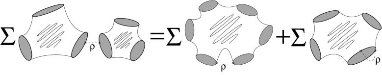
Figure 1: A diagrammatic representation of the quantum ${\cal A}_{\infty}$-relations (1) for $b=5$. The expansion in $g_{s}$, i.e., the sum over all genera $g$, is indicated by the wiggly lines on the Riemann surfaces.

The signs in (1) are:

$$s_{1} = \tilde{a}_{1}\!+\!\ldots\!+\!\tilde{a}_{k}\!+\!(\tilde{a}_{l\!+\!1}\!+\!\ldots\!+\!\tilde{a}_{m_{\sigma(1)}}\!+\!\tilde{A}_{\sigma(2)}\!+\!\ldots\tilde{A}_{\sigma(b\!-\!b^{\prime}+\!1)})(\tilde{d}\!+\!\tilde{a}_{k\!+\!1}\!+\!\ldots\!+\!\tilde{a}_{l}){}$$

$$s_{2} = \tilde{a}^{\prime}_{1}\!+\!\ldots\!+\!\tilde{a}^{\prime}_{k}\!+\!(\tilde{a}^{\prime}_{l\!+\!1}\!+\!\ldots\!+\!\tilde{a}^{\prime}_{m_{b^{\prime}}})(\tilde{d}\!+\!\tilde{a}^{\prime}_{k\!+\!1}\!+\!\ldots\!+\!\tilde{a}^{\prime}_{l})$$ (25)

$$s_{3} = \tilde{a}^{\prime}_{1}\!+\!\ldots\!+\!\tilde{a}^{\prime}_{k}\!+\!(\tilde{a}^{\prime\prime}_{1}\!+\!\ldots\!+\!\tilde{a}^{\prime\prime}_{l})(\tilde{a}^{\prime\prime}_{l\!+\!1}\!+\!\ldots\!+\!\tilde{a}^{\prime\prime}_{m_{b^{\prime\prime}}})\!+\!\tilde{A}_{b^{\prime\prime}}(\tilde{d}\!+\!\tilde{a}^{\prime}_{k\!+\!1}\!+\!\ldots\!+\!\tilde{a}^{\prime}_{m_{b^{\prime\prime}}}){}$$

$$s_{b^{\prime}} = \tilde{A}_{b^{\prime}}(\tilde{A}_{1}\!+\!\ldots\!+\!\tilde{A}_{b^{\prime}-1}){}\ .$$

and $s_{\sigma(\tilde{A})}$ is the Koszul sign for the permutation $\sigma\in S_{n}$ of boundary components with $\mathbb{Z}_{2}$-grading $\tilde{A}_{i}$. We used the abbreviations $a_{j}=a[\sigma(1)]_{j}$, $a^{\prime}_{j}=a[b^{\prime}]_{j}$ and $a^{\prime\prime}_{j}=a[b^{\prime\prime}]_{j}$. Fig. 1 shows a pictorial representation of the quantum ${\cal A}_{\infty}$-relations (1).

Cyclic invariance and unitality have been discussed earlier, so that it remains to show formula (1). We do this in several steps, starting with the insertion of the BRST operator in an arbitrary Riemann surface $\Sigma_{g,b}$. This causes a factorization of $\Sigma_{g,b}$ through degeneration channels where open or closed topological observables are exchanged through an infinitely long throat. These degenerations are described in terms of the boundary of the moduli space $\bar{\cal M}_{g,b;n,m_{1},\ldots,m_{b}}$ of a bordered Riemann surface $\Sigma_{g,b}$ with $n$ (dressed) punctures in the bulk and $m_{i}$ (dressed) punctures on the $i^{th}$ boundary. For a description of bordered Riemann surfaces and their moduli spaces in terms of symmetric Riemann surfaces the reader may consult [31]; see also [32, 33] for the context of open Gromov–Witten invariants.

An important observation will be that all the closed string degeneration channels vanish, provided that $m_{i}\geq 0$ for all $i=1,\ldots,b$. We will conclude that only the open string factorization channels give rise to the quantum ${\cal A}_{\infty}$-relations (1).

3.1 The boundary of the moduli space $\bar{\cal M}_{g,b;0,m_{1},\ldots,m_{b}}$

The proof of theorem 1 is more tractable if we start with the undeformed boundary theory, which means that we do not insert any bulk descendents in our amplitudes. After obtaining (1) in this situation we will include bulk deformations.

Our starting point is the amplitude

$$\int_{{\cal M}_{g,b}}d^{6g+3b-6}m~{}\bigl{\langle}\big{[}Q,\int\Psi_{A_{1}}\big{|}\ldots\big{|}\int\Psi_{A_{b}}\big{|}\prod_{i=1}^{6g+3b-6}G_{m_{i}}\big{]}\bigr{\rangle}_{\Sigma_{g,b}}=0\ ,$$ (26)

for $2g+b-2\geq 1$, $b\geq 1$, as depicted in Fig. 2. Here, we used the abbreviation

$$\int\Psi_{A_{i}}=\int_{{\cal M}^{i}_{m_{i}}}\Psi_{A_{i}}=P\int\psi_{a[i]_{1}}^{(1)}(\tau_{1})\ldots\int\psi_{a[i]_{m_{i}}}^{(1)}(\tau_{m_{i}})\ .$$ (27)

At this point some explanations on the moduli space in (26) are in order. ${\cal M}_{g,b}$ is the complex structure moduli space for $\Sigma_{g,b}$. On an internal point of this moduli space, that is, for a non-degenerate Riemann surface the boundary observables are integrated in cyclic order, i.e., the integration domain in (27) is

$${\cal M}^{i}_{m_{i}}=(\Delta_{m_{i}-1}\rightarrow S^{1})\ .$$

Here the simplex $\Delta_{m_{i}-1}$ is fibered over $S^{1}$ as follows:

$$\Delta_{m_{i}-1}=\left\{(\tau_{2},\ldots,\tau_{m_{i}})\big{|}\tau_{1}<\tau_{2}<\tau_{3}<\ldots<\tau_{m_{i}}<\tau_{1}+2\pi\right\}\ ,$$

where $\tau_{1}\in S^{1}$ with $\tau_{1}\simeq\tau_{1}+2\pi$. The total moduli space for a Riemann surface with punctures on the boundary is then a singular fibration

$${\cal M}_{g,b;0,m_{1},\ldots,m_{b}}=({\cal M}^{1}_{m_{1}}\times\ldots\times{\cal M}^{b}_{m_{b}})\rightarrow{\cal M}_{g,b}\ .$$

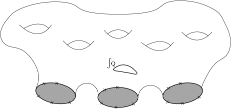
Figure 2: A genus 5 amplitude with three connected boundary component and a contour integral over the BRST current; the marked points indicate integrated boundary fields $\int\psi_{a_{i}}^{(1)}$. The Beltrami differential with the fermionic currents (4) are note depicted.

Having set up the basics about the moduli space, we investigate the effect of the BRST operator in (26). Relations (3) and (5) show that $Q$ gives rise to a total derivative on the moduli space. Using Stokes theorem the left-hand side of (26) looks like

$$\int_{\partial{\cal M}_{g,b;0,m_{1},\ldots,m_{b}}}\bigl{\langle}\ldots\bigr{\rangle}\ .$$

The boundary of the moduli space $\partial{\cal M}_{g,b;0,m_{1},\ldots,m_{b}}$ consists of singular configurations of the Riemann surface. This requires a compactification of the moduli space, $\overline{\cal M}_{g,b;0,m_{1},\ldots,m_{b}}$, meaning that well-defined configurations of Riemann surfaces are added at the singular locus of ${\cal M}_{g,b;0,m_{1},\ldots,m_{b}}$.

What kind of degenerations can occur when we deform the complex structure of the Riemann surface $\Sigma_{g,b}$, i.e., what are the boundary components of the moduli space, $\partial\overline{\cal M}_{g,b;0,m_{1},\ldots,m_{b}}$? To answer this let us divide the boundary configurations in three major classes:
(i) A sub-cylinder of $\Sigma_{g,b}$ becomes infinitely long and thin, so that we can insert a complete system of topological closed string observables.
(ii) A sub-strip of $\Sigma_{g,b}$ constricts to be infinitely long and we can insert a complete system of topological open string fields.
(iii) Several boundary fields come close together and we can take the topological operator product, which once again amounts to inserting a complete system of open string fields and bubbling of a disk. (This degeneration could be included in (ii), but we consider it separately for technical reasons, which become clear below.)

In the subsequent sections we investigate these three situations one-by-one and compute the resulting contributions to (1).

3.2 The closed string factorization channel

A factorization in the closed string channel (cf. Fig. 3) occurs if the BRST operator acts on one of the $G_{m_{i}}$’s and gives rise to the derivative $\frac{\partial}{\partial{m_{i}}}$. For definiteness let us first consider the situation like in Fig. 3a, where non of the factorization products is a disk.

In the neighborhood of the degeneration, the Riemann surface can be described in terms of the plumbing-fixture procedure [34, 35]. Take any two Riemann surfaces, $\Sigma_{1}$ and $\Sigma_{2}$, and cut out a disk of radius $\sqrt{|q|}$ on both of them, where $q\in\mathbb{C}$ and $|q|$ small. The centers of the disks are located at $\hat{z}_{1}$ and $\hat{z}_{2}$. Let us parameterize the neighborhood of the disks by the complex coordinates $z_{1}$ and $z_{2}$. The plumbing-fixture procedure tells us to glue the Riemann surfaces through the transition function $z_{2}-\hat{z}_{2}=q/(z_{1}-\hat{z}_{1})$. This gluing describes a cylinder of length $l$ and twist parameter $t$, determined by $q=e^{i\tau}=e^{-l+it}$. In the limit of infinite length, $l\rightarrow\infty$, the tube connects at the points, $\hat{z}_{1}$ and $\hat{z}_{2}$, to the Riemann surfaces, $\Sigma_{1}$ and $\Sigma_{2}$, respectively. Near this degenerate point the moduli space $\bar{\cal M}_{g,b;0,m_{1}\ldots m_{b}}$ can be parameterized by the coordinates $(\tau,\hat{z}_{1},\hat{z}_{2},\tilde{m}_{i},\hat{m}_{j})$. The moduli $\tilde{m}_{i}$ and $\hat{m}_{j}$ are the moduli on the Riemann surfaces $\Sigma_{1}$ and $\Sigma_{2}$.

Instead of putting the moduli dependence on $(\tau,\hat{z}_{1},\hat{z}_{2})$ into the world sheet metric and using the Beltrami differentials $\mu_{i}^{z}{}_{\bar{z}}$, let us make a local conformal transformation to a conformally flat metric on the cylinder and describe the moduli dependence through the transition function between the coordinates $z_{1}$ and $z_{2}$. An infinitesimal change of the moduli can then be written in terms of the conformal vector field

$$v^{z}(z_{1}-\hat{z}_{1})=\delta\hat{z}_{1}v_{1}+\delta\tau v_{\tau}+\delta\hat{z}_{2}v_{2}=\delta\hat{z}_{1}+\delta\tau(z_{1}-\hat{z}_{1})+\frac{\delta\hat{z}_{2}}{e^{i\tau}}(z_{1}-\hat{z}_{1})^{2}\ .$$

The integrals over the Beltrami differentials become

$$\int G_{m_{i}}=\oint_{\cal C}G_{zz}v^{z}_{i}+{\bar{G}}_{{\bar{z}}{\bar{z}}}\bar{v}^{\bar{z}}_{i}$$ (28)

for $i=1,2,\tau$. The cycle ${\cal C}$ wraps once around the tube.

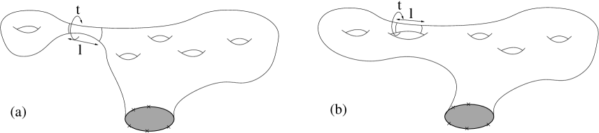
Figure 3: Closed string factorizations

The degeneration that we described here corresponds to the situation when $Q$ acts on $G_{l}$ and gives rise to the total derivative $\frac{\partial}{\partial{l}}$. Using (28) the amplitude on the degenerate Riemann surface becomes

$$\lim_{l\rightarrow\infty}\int\bigl{\langle}\ldots[G_{-1},[{\bar{G}}_{-1},\phi_{m}(\hat{z}_{1})]]\prod_{i=1}^{6g^{\prime}+3b^{\prime}-6}G_{\tilde{m}_{i}}\bigr{\rangle}_{\Sigma_{g^{\prime},b^{\prime}}}~{}\eta^{mn}~{}\times$$

$$\times \bigl{\langle}\,\phi_{n}\,\big{|}q^{L_{0}}\bar{q}^{\bar{L}_{0}}\big{|}\,\phi_{k}\,\bigr{\rangle}\eta^{kl}~{}\int\bigl{\langle}[i(G_{0}-{\bar{G}}_{0}),[G_{-1},[{\bar{G}}_{-1},\phi_{l}(\hat{z}_{2})]]]\ldots\prod_{j=1}^{6g^{\prime\prime}+3b^{\prime\prime}-6}G_{\hat{m}_{j}}\bigr{\rangle}_{\Sigma_{g^{\prime\prime},b^{\prime\prime}}}\ ,$$

where $g^{\prime}+g^{\prime\prime}=g$, $b^{\prime}+b^{\prime\prime}=b$. We omitted the details about the integration over the moduli spaces and also about the boundary observables, which are indicated by dots. In the limit $l\rightarrow\infty$, $q$ vanishes and only states with $L_{0}=\bar{L}_{0}=0$, i.e., the topological closed string observables survive, so that $\eta^{mn}$ restricts to the inverse of the topological closed string metric.

The important point is then that the zero mode $G_{0}\!-\!{\bar{G}}_{0}$ remains in (3.2) and acts on the bulk observable, so that the whole expression vanishes by the gauge condition (2). A similar argument applies to the factorization channel of Fig. 3b, which therefore vanishes too.

Recall that we excluded so far the situation where one of the two Riemann surfaces, $\Sigma_{1}$ or $\Sigma_{2}$, is a disk. Let us consider this case now. Other than before there is no twist parameter $t$, so that the factorization becomes

$$\int\bigl{\langle}\ldots[G_{-1},[{\bar{G}}_{-1},\phi_{m}(\hat{z}_{1})]]\prod_{i=1}^{6g+3b-9}G_{\tilde{m}_{i}}\bigr{\rangle}_{\Sigma_{g,b-1}}~{}\eta^{mn}~{}\bigl{\langle}\phi_{n}(\hat{z}_{2})\int\Psi_{A_{i}}\bigr{\rangle}_{\Sigma_{0,1}}\ .$$ (30)

Notice that $i(G_{0}-{\bar{G}}_{0})$ does not appear because of the absence of the twist parameter $t$, and there is no $[G_{-1},[{\bar{G}}_{-1},\phi_{l}]]$ associated to the modulus $\hat{z}_{2}$ either, which reflects the fact that the disk has a conformal Killing vector field that can be used to fix $\hat{z}_{2}$. Let us use now our assumption that we have at least one insertion of an observable on each boundary, i.e., $m_{i}\geq 1$. In [6] it was then shown that a disk amplitude like the one in (30) vanishes in view of a conformal Ward identity. We conclude that, for $m_{i}\geq 1$, factorizations in the closed string channel do not contribute at all to the quantum ${\cal A}_{\infty}$-structure (1).

3.3 Boundaries without observables – non-stable configurations

Let us briefly comment on the case $m_{i}=0$. The expression (30) becomes

$$\int\bigl{\langle}\ldots[G_{-1},[{\bar{G}}_{-1},\phi_{m}(\hat{z}_{1})]]\prod_{i=1}^{6g+3b-9}G_{\tilde{m}_{i}}\bigr{\rangle}_{\Sigma_{g,b-1}}~{}\eta^{mn}~{}\bigl{\langle}\phi_{n}(\hat{z}_{2})\bigr{\rangle}_{\Sigma_{0,1}}\ ,$$ (31)

which corresponds to a non-stable configuration, because the conformal Killing vector that rotates the disk is not fixed. The simplest example for such a situation is the factorization of the annulus amplitude, i.e.,

$$\int_{0}^{\infty}\!\!dL~{}\bigl{\langle}\left[Q,~{}{1\!\!\!\!1\,}~{}|~{}.~{}|~{}G_{L}\right]\bigr{\rangle}_{\Sigma_{0,2}}=0\ .$$ (32)

The open string factorization channel gives the Witten index, or intersection number,

$$\sum_{a,b}{\cal F}_{{1\!\!\!\!1\,}ab}\rho^{ab}=-{\rm Tr}_{{\cal H}^{\alpha\beta}_{op}}(-)^{F}\ ,$$ (33)

where we used the equation in the unitality properties (21) that relates 3-point functions to the topological metric. The closed string channel gives

$$\bigl{\langle}\phi_{m}~{}{1\!\!\!\!1\,}\bigr{\rangle}_{\Sigma_{0,1}}~{}\eta^{mn}\bigl{\langle}\phi_{n}\bigr{\rangle}_{\Sigma_{0,1}}\ ,$$

so that the factorization of the annulus amplitude (32) can be interpreted as topological Cardy relation of 2d topological field theory [27, 28]. In general, one should be cautious about considering factorizations that involve non-stable configurations like (31). They indicate ambiguities related to divergences in topological amplitudes (cf. [9]).

3.4 The open string factorization channels

Let us turn now to the non-vanishing contributions to the quantum ${\cal A}_{\infty}$ relations (1), which come from open string factorization channels. Factorizations in the open string channel corresponding to an infinitely long strip are shown in Fig. 4.

The left-hand side of the quantum ${\cal A}_{\infty}$-relation (1)

We consider the situation in Fig. 4a first. Locally near the degeneration point the moduli space can be parameterized by $(l,\hat{x}_{1},\hat{x}_{2},\tilde{m}_{1},\ldots,\tilde{m}_{3|\tilde{\chi}|},\hat{m}_{1},\ldots,\hat{m}_{3|\hat{\chi}|})$. The first three coordinates parameterize the length $l$ of the strip as well as the positions $\hat{x}_{1}$ and $\hat{x}_{2}$ of the punctures, where the strip ends on the surface boundaries. $\tilde{m}_{i}$ and $\hat{m}_{j}$ are the moduli of the resulting Riemann surfaces $\Sigma_{g^{\prime},b^{\prime}}$ and $\Sigma_{g^{\prime\prime},b^{\prime\prime}}$, respectively. Here, $g^{\prime}+g^{\prime\prime}=g$ and $b^{\prime}+b^{\prime\prime}=b+1$. Since $Q$ acted on $G_{l}$ we have to evaluate $l$ at infinity. The Beltrami differentials associated to the moduli $\hat{x}_{1}$ and $\hat{x}_{2}$ localize around the punctures as before. The channel in Fig. 4a gives

$$(-)^{3|\tilde{\chi}|}\lim_{l\rightarrow\infty}\bigl{\langle}\int\Psi_{A_{1}}\ldots\int\Psi_{A_{b}}\big{|}\int_{\tilde{\cal M}_{g^{\prime},b^{\prime}}}d^{3|\tilde{\chi}|}\tilde{m}~{}\prod_{i=1}^{3|\tilde{\chi}|}G_{\tilde{m}_{i}}\int_{\hat{x}_{1}}G_{\hat{x}_{1}}\int_{\hat{x}_{2}}G_{\hat{x}_{2}}\int_{\hat{\cal M}_{g^{\prime\prime},b^{\prime\prime}}}d^{3|\hat{\chi}|}\hat{m}~{}\prod_{i=1}^{3|\hat{\chi}|}G_{\hat{m}_{i}}\bigr{\rangle}\ .$$ (34)

The sign comes from pulling $Q$ through all the operators. We used $\tilde{A}_{1}+\ldots+\tilde{A}_{b}=1$. Notice that contributions with $(g^{\prime},b^{\prime})=(0,1)$ or $(g^{\prime\prime},b^{\prime\prime})=(0,1)$ vanish, because the degeneration results into disk amplitudes that vanish by a conformal Ward identity [6].

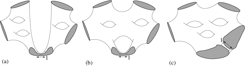
Figure 4: Open string factorizations through infinitely long strips.

We have not decided yet, which boundary component, that is to say, which fields $\Psi_{A_{i}}$ are involved in the factorization. Let us pick $\Psi_{A_{1}}$ first and take care of all other boundaries afterwards. The boundary observables are, after factorization, split into a collection $\psi^{(1)}_{a_{l+1}}\ldots\psi^{(1)}_{a_{k}}$ on $\Sigma_{g^{\prime\prime},b^{\prime\prime}}$ and $\psi^{(1)}_{a_{k+1}}\ldots\psi^{(1)}_{a_{m_{1}}}\psi^{(1)}_{a_{1}}\ldots\psi^{(1)}_{a_{l}}$ on $\Sigma_{g^{\prime},b^{\prime}}$, where $l,k=1,\ldots,m_{1}$ with $l\leq k$. In order to avoid over-counting we take $\psi^{(1)}_{a_{1}}$ always to be on $\Sigma_{g^{\prime},b^{\prime}}$.

There is another choice that determines how the remaining fields $\Psi_{A_{i}}$ for $i=2,\ldots,b$ are distributed among $\Sigma_{g^{\prime},b^{\prime}}$ and $\Sigma_{g^{\prime\prime},b^{\prime\prime}}$. We pick again the simplest choice: $\Sigma_{g^{\prime},b^{\prime}}$ carries the fields $\Psi_{A_{i}}$ for $i=2,\ldots,b^{\prime}$ and $\Sigma_{g^{\prime\prime},b^{\prime\prime}}$ carries $\Psi_{A_{i}}$ for $i=b^{\prime}+1,\ldots,b$.

Reshuffling the operators and inserting a complete system of boundary observables gives

$${}(-)^{s}\rho^{cd} \bigl{\langle}\int\psi^{(1)}_{a_{l+1}}\ldots\psi^{(1)}_{a_{k}}\big{|}\int\Psi_{A_{2}}\ldots\int\Psi_{A_{b^{\prime}}}\big{|}\int_{\tilde{\cal M}_{g^{\prime},b^{\prime}}}d^{3|\tilde{\chi}|}\tilde{m}~{}\prod_{i=1}^{3|\tilde{\chi}|}G_{\tilde{m}_{i}}\int_{\hat{x}_{1}}G_{\hat{x}_{1}}\psi_{c}(\hat{x}_{1})\bigr{\rangle}_{\Sigma_{g^{\prime},b^{\prime}}}\times$$

$${}\times \bigl{\langle}\psi_{d}(\hat{x}_{2})\int\psi^{(1)}_{a_{k+1}}\ldots\psi^{(1)}_{a_{l}}\big{|}\int\Psi_{A_{b^{\prime}+1}}\ldots\int\Psi_{A_{b}}\big{|}\int_{\hat{x}_{2}}G_{\hat{x}_{2}}\int_{\tilde{\cal M}_{g^{\prime\prime},b^{\prime\prime}}}d^{3|\hat{\chi}|}\hat{m}~{}\prod_{i=1}^{3|\hat{\chi}|}G_{\hat{m}_{i}}\bigr{\rangle}_{\Sigma_{g^{\prime\prime},b^{\prime\prime}}}\ .$$

The sign is $s=1\!+\!(3|\tilde{\chi}|\!+\!1)\tilde{d}\!+\!(\tilde{a}_{1}\!+\!\ldots\!+\!\tilde{a}_{l})(\tilde{a}_{l\!+\!1}\!+\!\ldots\!+\!\tilde{a}_{m_{1}})\!+\!(\tilde{A}_{2}\!+\!\ldots\!+\!\tilde{A}_{b^{\prime}})(\tilde{a}_{k\!+\!1}\!+\!\ldots\!+\!\tilde{a}_{l})$.

Now we use the fact that the Beltrami differentials associated to the positions $\hat{x}_{i}$ localize around the punctures: $\int_{\hat{x}_{1}}G_{\hat{x}_{1}}\psi_{c}(\hat{x}_{1})\rightarrow\int_{\hat{x}_{1}}\psi_{c}^{(1)}$. Further reshuffling of fields and using the definition of topological amplitudes in (7) we obtain

$$(-)^{s_{1}}\rho^{cd}{\cal F}^{g^{\prime\prime},b^{\prime\prime}}_{a_{1}\ldots a_{k}ca_{l+1}\ldots a_{m_{1}}|A_{2}|\ldots|A_{b^{\prime}}}{\cal F}^{g^{\prime},b^{\prime}}_{da_{k+1}\ldots a_{l}|A_{b^{\prime}+1}|\ldots|A_{b}}\ ,$$ (35)

where

$$s_{1}=\tilde{a}_{1}\!+\!\ldots\!+\!\tilde{a}_{k}\!+\!(\tilde{a}_{l\!+\!1}\!+\!\ldots\!+\!\tilde{a}_{m_{1}}\!+\!\tilde{A}_{2}\!+\!\ldots\tilde{A}_{b^{\prime}})(\tilde{d}\!+\!\tilde{a}_{k\!+\!1}\!+\!\ldots\!+\!\tilde{a}_{l})\ .$$

In order to take into account the factorizations involving the other boundary components and all the inequivalent distributions of remaining fields $\int\Psi_{A_{i}}$, we exchange the observables $\int\Psi_{A_{i}}$ according to an element $\sigma$ in the symmetric group $S_{b}$. This gives rise to the Koszul sign $(-)^{s_{\sigma(\tilde{A})}}$. Then, summing up all factorization channels gives

$$\sum_{g^{\prime}=0}^{g}{}^{{}^{\prime}}\sum_{b^{\prime}=1}^{b}{}^{{}^{\prime}} \sum_{\sigma\in S_{b}}\sum_{l\leq k=1}^{m_{\sigma(1)}}\frac{(-)^{s_{\sigma(\tilde{A})}+s_{1}}}{(b\!-\!b^{\prime})!(b^{\prime}\!-\!1)!}\times$$

$$\times {\cal F}^{g^{\prime},b-b^{\prime}+1}_{a_{1}\ldots a_{l}ca_{k\!+\!1}\ldots a_{m_{\sigma(1)}}|A_{\sigma(2)}|\ldots|A_{\sigma(b\!-\!b^{\prime}\!+\!1)}}\rho^{cd}{\cal F}^{g-g^{\prime},b^{\prime}}_{da_{l\!+\!1}\ldots a_{k}|A_{\sigma(b\!-\!b^{\prime}\!+\!2)}|\ldots|A_{\sigma(b)}}{}\ .$$

The factor $[(b\!-\!b^{\prime})!(b^{\prime}\!-\!1)!]^{-1}$ accounts for over-counting, and $\sum{}^{{}^{\prime}}$ means that $(g^{\prime},b^{\prime})=(0,b)$ and $(g^{\prime},b^{\prime})=(g,1)$ are not included in the sum. In fact, the latter contributions come from class (iii) in our list of degenerations in section 3.1. Let us briefly consider those before we proceed to Fig. 4b.

When $Q$ acts on the integrated descendents $\int\psi_{a}^{(1)}$, it acts as a boundary operator on one of the fiber components ${\cal M}^{i}_{m_{i}}$ of the moduli space $\bar{\cal M}_{g,b;0,m_{1}\ldots m_{b}}$. The boundary of ${\cal M}^{i}_{m_{i}}$ corresponds to situations where two or more observables collide. So we have to sum over all possible contact terms of boundary observables. This is exactly the same effect that gave rise to the (classical) ${\cal A}_{\infty}$-structure for disk amplitudes in [6]. If, for instance, the fields $\psi_{a_{l+1}}$ through $\psi_{a_{k}}$ for $l,k=1,\ldots,m_{i}$ and $l+2\leq k$, come together very closely a disk with these fields bubbles off and we get

$$-(-)^{\tilde{a}_{1}+\ldots+\tilde{a}_{k-1}} \bigl{\langle}\psi_{a_{1}}^{(1)}\ldots\psi_{a_{l}}^{(1)}\psi_{c}^{(1)}\psi_{a_{k+1}}^{(1)}\ldots\psi_{a_{m_{1}}}^{(1)}|\int\Psi_{A_{2}}\ldots|\prod_{j=1}^{6g+3b-6}G_{\tilde{m}_{j}}\bigr{\rangle}_{\Sigma_{g,b}}\times{}$$ (37)

$$\times~{}\omega^{cd}\bigl{\langle}\psi_{d}\psi_{a_{l+1}}\psi_{a_{l+2}}^{(1)}\ldots\psi_{a_{k-1}}^{(1)}\psi_{a_{k}}\bigr{\rangle}_{\Sigma_{0,1}}\ ,$$

and similarly

$$-(-)^{s} \bigl{\langle}\psi_{a_{1}}\psi_{a_{2}}\psi_{a_{3}}^{(1)}\ldots\psi_{a_{l}}^{(1)}\psi_{c}^{(1)}\psi_{a_{k+1}}^{(1)}\ldots\psi_{a_{m_{1}-1}}^{(1)}\psi_{a_{m_{1}}}\bigr{\rangle}_{\Sigma_{0,1}}\times$$

$$\times~{}\omega^{cd}\bigl{\langle}\psi_{d}^{(1)}\psi_{a_{l+1}}^{(1)}\ldots\psi_{a_{k}}^{(1)}|\int\Psi_{A_{2}}\ldots|\prod_{j=1}^{6g+3b-6}G_{\tilde{m}_{j}}\bigr{\rangle}_{\Sigma_{g,b}}{}\ ,$$

where $s=\tilde{a}_{m_{1}}+\tilde{a}_{2}+\ldots+\tilde{a}_{l}+(\tilde{a}_{k+1}+\ldots+\tilde{a}_{m_{1}})(\tilde{d}+\tilde{a}_{l+1}+\ldots+\tilde{a}_{k})$. When we compare these expressions with (35) taking into account the sign in (10), we see immediately that they provide exactly the two missing terms with $(g^{\prime},b^{\prime})=(0,b)$ and $(g^{\prime},b^{\prime})=(g,1)$ in (3.4).

The all-genus amplitudes (14) allow us to combine the factorizations that we have studied so far into the left-hand side of (1).

The right-hand side of the quantum ${\cal A}_{\infty}$-relation (1)

The channel shown in Fig. 4b gives a degeneration resulting in a single Riemann surface $\Sigma_{g-1,b+1}$, that is, one boundary component splits into two, thus increasing the number of boundaries by one and decreasing the genus by one. We rearrange the boundary components in the amplitude such that the observables $\Psi_{A_{b^{\prime}}}$, which are effected by the degeneration, are at the first position. This gives rise to the sign $s_{b^{\prime}}$ defined in (3). The observables are split into $\psi^{(1)}_{a^{\prime}_{l+1}}\ldots\psi^{(1)}_{a^{\prime}_{k}}$ and $\psi^{(1)}_{a^{\prime}_{k+1}}\ldots\psi^{(1)}_{a^{\prime}_{m_{b^{\prime}}}}\psi^{(1)}_{a^{\prime}_{1}}\ldots\psi^{(1)}_{a^{\prime}_{l}}$. Here, $a^{\prime}_{i}=a[b^{\prime}]_{i}$. In the limit $l\rightarrow\infty$ the amplitude becomes

$${}(-)^{s+s_{b^{\prime}}}\rho^{cd}\bigl{\langle}\psi_{c}(\hat{x}_{1})\int\psi^{(1)}_{a^{\prime}_{k+1}}\ldots\psi^{(1)}_{a^{\prime}_{l}} \big{|} \int\psi^{(1)}_{a^{\prime}_{l+1}}\ldots\psi^{(1)}_{a^{\prime}_{k}}\big{|}\int\Psi_{A_{1}}\ldots\big{|}\psi_{d}(\hat{x}_{2})\times$$

$$\times \int_{\hat{x}_{1}}\!\!G_{\hat{x}_{1}}\!\!\int_{\hat{x}_{2}}\!\!G_{\hat{x}_{2}}\!\!\int_{\tilde{\cal M}_{g-1,b+1}}d^{3|\tilde{\chi}|}\tilde{m}\prod_{j=1}^{3|\tilde{\chi}|}G_{\tilde{m}_{j}}\bigr{\rangle}_{\Sigma_{g-1,b+1}}\ ,$$

where $s=(\tilde{a}^{\prime}_{l+1}+\ldots+\tilde{a}^{\prime}_{m_{b^{\prime}}})(\tilde{a}^{\prime}_{1}+\ldots+\tilde{a}^{\prime}_{l})$.

We commute $\psi_{c}$ and $\psi_{d}$ through the other fields to their ’right’ positions and make use of the localization $\int_{\hat{x}_{1}}G_{\hat{x}_{1}}\psi_{c}\rightarrow\int_{\hat{x}_{1}}\psi_{c}^{(1)}$. After further reshuffling of the observables and using (7) we obtain:

$$-(-)^{s_{b^{\prime}}+s_{2}}\rho^{cd}~{}{\cal F}^{g-1,b+1}_{a^{\prime}_{1}\ldots a^{\prime}_{l}ca^{\prime}_{k+1}\ldots a^{\prime}_{m_{b}^{\prime}}|da^{\prime}_{l+1}\ldots a^{\prime}_{k}|A_{1}|\ldots|\hat{A}_{b^{\prime}}|\ldots|A_{b}}\ ,$$

where the signs can be found in (3). Summing over all such channels yields

$$-\sum_{b^{\prime}=1}^{b}\sum_{l\leq k=1}^{m_{b^{\prime}}}(-)^{s_{b^{\prime}}+s_{2}}\rho^{cd}~{}{\cal F}^{g-1,b+1}_{a^{\prime}_{1}\ldots a^{\prime}_{l}ca^{\prime}_{k+1}\ldots a^{\prime}_{m_{b}^{\prime}}|da^{\prime}_{l+1}\ldots a^{\prime}_{k}|A_{1}|\ldots|\hat{A}_{b^{\prime}}|\ldots|A_{b}}\ ,$$ (39)

which provides the (undeformed) first term on the right-hand side of (1).

Finally we have to look at the degeneration in Fig. 4c, where the genus $g$ stays the same and two boundary components join into one. Let us pick the fields $\Psi_{A_{b^{\prime\prime}}}$ and $\Psi_{A_{b^{\prime}}}$ on the colliding boundaries, where $b^{\prime},b^{\prime\prime}=1,\ldots,b$ and $b^{\prime\prime}<b^{\prime}$. Pulling these observables through the other fields to the first two positions in the amplitude gives the sign $s_{b^{\prime\prime}}+s_{b^{\prime}}$. In the degeneration limit we insert the complete system $\rho^{cd}\psi_{c}\psi_{d}$ in such a way that $\psi_{c}$ is located between $\psi^{(1)}_{a^{\prime}_{k}}$ and $\psi^{(1)}_{a^{\prime\prime}_{l+1}}$, whereas $\psi_{d}$ is located between $\psi^{(1)}_{a^{\prime\prime}_{l}}$ and $\psi^{(1)}_{a^{\prime}_{k+1}}$. Here $k=1,\ldots,m_{b^{\prime}}$ and $l=1,\ldots,m_{b^{\prime\prime}}$. We obtain:

$${}(-)^{s+s_{b^{\prime}}+s_{b^{\prime\prime}}}\rho^{cd}\bigl{\langle}\psi_{c}(\hat{x}_{1}) \int\psi^{(1)}_{a^{\prime}_{k+1}}\ldots\psi^{(1)}_{a^{\prime}_{m_{b^{\prime}}}}\psi^{(1)}_{a^{\prime}_{1}}\ldots\psi^{(1)}_{a^{\prime}_{k}}\int\psi^{(1)}_{a^{\prime\prime}_{l+1}}\ldots\psi^{(1)}_{a^{\prime}_{m_{b^{\prime\prime}}}}\psi^{(1)}_{a^{\prime\prime}_{1}}\ldots\psi^{(1)}_{a^{\prime\prime}_{l}}\big{|}\times$$

$$\times \int\Psi_{A_{1}}\ldots\big{|}\psi_{d}(\hat{x}_{2})\int_{\hat{x}_{1}}\!\!G_{\hat{x}_{1}}\!\!\int_{\hat{x}_{2}}\!\!G_{\hat{x}_{2}}\!\!\int_{\tilde{\cal M}_{g,b-1}}d^{3|\tilde{\chi}|}\tilde{m}\prod_{j=1}^{3|\tilde{\chi}|}G_{\tilde{m}_{j}}\bigr{\rangle}_{\Sigma_{g,b-1}}\ ,$$

where $\psi_{c}$ and $\psi_{d}$ are not yet at the positions according to their boundary condition labels. The sign is $s\!=\!(\tilde{a}^{\prime}_{1}\!+\!\ldots\!+\!\tilde{a}^{\prime}_{k})(\tilde{a}^{\prime}_{k\!+\!1}\!\!+\!\ldots\!+\!\tilde{a}^{\prime}_{m_{b^{\prime}}})\!+\!(\tilde{a}^{\prime\prime}_{1}\!+\!\ldots\!+\!\tilde{a}^{\prime\prime}_{l})(\tilde{a}^{\prime\prime}_{l\!+\!1}\!\!+\!\ldots\!+\!\tilde{a}^{\prime\prime}_{m_{b^{\prime\prime}}})$. Following the same steps as for the other factorizations and collecting all contributions we obtain:

$$-\sum_{b^{\prime\prime}<b^{\prime}=1}^{b}\sum_{k=1}^{m_{b^{\prime}}}\sum_{l=1}^{m_{b^{\prime\prime}}}(-)^{s_{b^{\prime}}+s_{b^{\prime\prime}}+s_{3}}\rho^{cd}{\cal F}^{g,b-1}_{a^{\prime}_{1}\ldots a^{\prime}_{k}ca^{\prime\prime}_{l+1}\ldots a^{\prime\prime}_{m_{b^{\prime\prime}}}a^{\prime\prime}_{1}\ldots a^{\prime\prime}_{l}da^{\prime}_{k+1}\ldots a^{\prime}_{m_{b^{\prime}}}|A_{1}\ldots\hat{A}_{b^{\prime\prime}}\ldots\hat{A}_{b^{\prime}}\ldots A_{b}}\ .$$ (40)

This provides the final contribution to the quantum ${\cal A}_{\infty}$ relation (1). Actually, what we have found so far are the undeformed, minimal quantum ${\cal A}_{\infty}$-relations for the undeformed amplitudes ${\cal F}^{b}_{A_{1}|\ldots|A_{b}}(g_{s};t=0)$, in particular, ${\cal F}^{0,1}_{a}(t=0)={\cal F}^{0,1}_{ab}(t=0)=0$.

Remarks: Observe that the restriction $m_{i}=0$ for $i=1,\ldots,b$ did not play any rôle in the analysis of the open string factorization channels. This means that in situations with ’bare’ boundary components, the quantum ${\cal A}_{\infty}$-relations (1) hold only up to non-stable configurations like (30).

Strictly speaking, we are not done with the factorizations of the undeformed amplitudes yet, because the annulus amplitude, equation (12) with $Q$ insertion and $t=0$, was not included in our considerations so far. We just state here that the gymnastics of the previous section can be applied as well and leads to the still missing terms in (1).

3.5 Including closed string deformations

The inclusion of closed string deformations, i.e., insertions of bulk observables in the amplitudes, has a quite trivial effect. First of all, contact terms between bulk fields do not contribute if the regularization is chosen appropriately (cf. [6]).

Suppose we insert one (integrated) bulk descendent in the amplitude (26). If $Q$ acts on boundary fields or the $G_{m_{i}}$’s we obtain the same factorization channels as before. In the case (35), where the Riemann surface splits into two, $\Sigma_{1}$ and $\Sigma_{2}$, the integration over the bulk observable splits too, i.e., $\int_{\Sigma}\phi_{i}^{(2)}\rightarrow\int_{\Sigma_{1}}\phi_{i}^{(2)}+\int_{\Sigma_{2}}\phi_{i}^{(2)}$. Notice that this is consisted with, and therefore allows, the formal integration of bulk descendents to the deformed amplitudes (7).

If $Q$ acts, on the other hand, on the bulk descendent we get contact terms between this bulk descendent and boundary fields, which gives rise to disks that bubble off the Riemann surface (cf. [6]). This provides additional contributions for the quantum ${\cal A}_{\infty}$-relations involving ${\cal F}^{0,1}_{a}(t)$ and ${\cal F}^{0,1}_{ab}(t)$.

We conclude that the closed string observables deform the minimal quantum ${\cal A}_{\infty}$-structure for undeformed amplitudes into the weak quantum ${\cal A}_{\infty}$-structure (1) for deformed amplitudes.

4 Comments on the quantum ${\cal A}_{\infty}$-relations

So far we have neglected the boundary condition labels, $\alpha,\ldots$ for convenience. Reintroducing them makes apparent that relation (1) defines a cyclic, unital quantum ${\cal A}_{\infty}$ category (rather than an algebra). It is the quantum version of a (classical) ${\cal A}_{\infty}$-category, which was originally introduced in [16]. The boundary conditions (or D-branes) are the objects, $\alpha,\beta,\ldots\in Obj({{\cal A}^{q}_{\infty}})$, and the boundary observables are the morphisms, $\psi^{\alpha\beta}_{a}\in Hom_{{\cal A}^{q}_{\infty}}(\alpha,\beta)={\cal H}^{\alpha\beta}_{op}$. The formulation of the classical ${\cal A}_{\infty}$-relations in terms of scattering products $r_{n}:{\cal H}^{\alpha_{1}\alpha_{2}}_{op}\otimes\ldots\otimes{\cal H}^{\alpha_{n}\alpha_{n\!+\!1}}_{op}\rightarrow{\cal H}^{\alpha_{1}\alpha_{n\!+\!1}}_{op}$ can be found in the literature. We refer to the recent review [4] on this subject, and references therein.

Instead of elaborating on this issue we want to focus subsequently on the rôle and the effects of the charge selection rule on the quantum ${\cal A}_{\infty}$-relations (1) in models with ${\hat{c}}=3$. For this purpose let us distinguish between boundary condition preserving observables (BPO) $\psi^{\alpha\alpha}_{a}\in{\cal H}^{\alpha\alpha}_{op}$ and boundary condition changing observables (BCO) $\psi^{\alpha\beta}_{a}\in{\cal H}^{\alpha\beta}_{op}$ for $\alpha\neq\beta$.

Consider a single D-brane so that we have only BPOs. We assume to be in a model where the boundary condition preserving sector has only integral $U(1)$ charges, i.e., $q=0,1,2,3$, and the unique observable of charge $0$ is the unit operator ${1\!\!\!\!1\,}$. This is the case in most models of interest.

It was pointed out in [8] that the disk amplitudes then have a particularly simple form and that the (classical) ${\cal A}_{\infty}$-relations are trivially satisfied. A similar argument can be adopted to the all-genus topological string amplitudes ${\cal F}^{b}_{A_{1}|\ldots|A_{b}}$ and goes as follows: Recall first that for ${\hat{c}}=3$ the charge selection rule (16) is the same irrespective of the Euler character of the Riemann surface. In particular, the selection rule (16) admits to insert only marginal boundary observables in the amplitude ${\cal F}^{b}_{A_{1}|\ldots|A_{b}}$ and moreover an arbitrary number of them. Take such an amplitude and substitute one of the marginal observables by a charge $2$ (or $3$) one. In order to obtain a non-vanishing amplitude the selection rule (16) forces us to introduce one (or two) units ${1\!\!\!\!1\,}$ in the amplitude. On the other hand, by the unitality property (21) the only non-vanishing amplitudes with unit are disk 3-point correlators. We conclude that amplitudes on a single D-brane (with the above assumptions) (i) have only marginal insertions or (ii) are given by ${\cal F}^{0,1}_{{1\!\!\!\!1\,}ab}$. From this observation it follows readily that the quantum ${\cal A}_{\infty}$-relations (1) are trivially satisfied when we consider a single D-brane.

Only in multiple D-brane situations, that is for a quantum ${\cal A}_{\infty}$-category, the algebraic equations (1) give non-trivial relations and can be used as constraints on the amplitudes. In fact, they provide a means of determining higher genus multiple-boundary amplitudes ${\cal F}^{g,b}_{A_{1}|\ldots|A_{b}}$ recursively from amplitudes with larger Euler character. To see this let us rewrite (1) in such a way that they look diagrammatically as follows:

$$\parbox{119.50148pt}{\epsfbox{recursive1.eps}}(\textrm{amplitudes with}\ \chi>\chi_{g,b})\ .$$ (41)

Here, as compared to (1), we gave up combining the different levels of genera $g$ into an expansion of the topological string coupling $g_{s}$. The left-hand side of (41) comprises all terms from the left-hand side of (1) that involve disk amplitudes. Therefore, writing the quantum ${\cal A}_{\infty}$-relations in the form (41) makes apparent that they provide a sequence of linear systems in ${\cal F}^{g,b}_{A_{1}|\ldots|A_{b}}$, which can be solved recursively, starting from disk amplitudes.

5 Quantum master equation?

From string field theory [30, 10] it is known that the classical as well as the quantum ${\cal A}_{\infty}$-structure have a dual description on a (formal) noncommutative supermanifold. In our context the latter corresponds to the open string moduli space (see [11] for the precise relation) and we should be able to recast the quantum ${\cal A}_{\infty}$-relations (1) into a quantum master equation on moduli space.

In order to see whether this is indeed true let us introduce for our basis $\psi^{\alpha\beta}_{a}\in{\cal H}^{\alpha\beta}_{op}$ a dual basis $\hat{s}^{\alpha\beta}_{a}\in{\cal H}_{op}^{d}$. The deformation parameters (or open string moduli) $\hat{s}^{\alpha\beta}_{a}$ are taken to be associative and graded noncommutative. The latter requirement accounts for cases where we have Chan–Paton extensions in the boundary sector [11], i.e., the deformation parameters are (super)matrices $X_{a}$. The $\mathbb{Z}_{2}$-degree of $\hat{s}^{\alpha\beta}_{a}$ is the same as the $\mathbb{Z}_{2}$-degree of $\psi^{\alpha\beta}_{a}$. Let us drop the boundary condition labels again, understanding that the deformation parameters correspond to edges in some Quiver diagram associated to the D-brane configuration [11].

An element in the ring $A$ of (formal) power series in $\{\hat{s}_{a}\}$ is given by $f(\hat{s}_{a})=f_{0}+\sum_{m=1}^{\infty}\frac{1}{m}f_{a_{1}\ldots a_{m}}\hat{s}_{a_{1}}\ldots\hat{s}_{a_{m}}$. Let us define left and right partial derivatives $\stackrel{{\scriptstyle\rightharpoonup}}{{\partial}}_{a}$, $\stackrel{{\scriptstyle\leftharpoonup}}{{\partial}}_{a}:A\rightarrow A$ by:

$${}\stackrel{{\scriptstyle\rightharpoonup}}{{\partial}}_{a}f(s) = (-)^{\tilde{a}(\tilde{f}+1)}f(s)\stackrel{{\scriptstyle\leftharpoonup}}{{\partial}}_{a}=$$

$$= \sum_{m=0}^{\infty}\sum_{i=1}^{m}(-)^{\tilde{a}(\tilde{a}_{1}+\ldots+\tilde{a}_{i-1})}f_{a_{1}\ldots a_{i-1}aa_{i+2}\ldots a_{m}}\hat{s}_{a_{1}}\ldots\hat{s}_{a_{i-1}}\hat{s}_{a_{i+1}}\ldots\hat{s}_{a_{m}}\ ,$$

and the BV operator $\Delta:A\rightarrow A$ by:

$$\Delta:=\rho^{ab}\stackrel{{\scriptstyle\rightharpoonup}}{{\partial}}_{a}\stackrel{{\scriptstyle\rightharpoonup}}{{\partial}}_{b}\ .$$

Consider the formal power series

$$g_{s}^{-2}S(g_{s},t,\hat{s}):=\sum_{b=1}^{\infty}\sum_{m_{i}=0}^{\infty}\frac{1}{b!m_{1}\ldots m_{b}}{\cal F}^{b}_{A_{1}|\ldots|A_{b}}(g_{s},t)~{}\hat{s}_{A_{1}}\ldots\hat{s}_{A_{b}}$$ (42)

associated to the all-genus topological string amplitudes (14), where we used the abbreviation $\hat{s}_{A_{i}}=\hat{s}_{a[i]_{1}}\ldots\hat{s}_{a[i]_{m_{i}}}$. Note that amplitudes with $m_{i}=0$ are included in the series (42). It is understood that $1/{m_{i}}$ is substituted by $1$ whenever $m_{i}=0$. From the $\mathbb{Z}_{2}$-selection rule (18) it follows that the series $S(g_{s},t,\hat{s})$ has even degree.

After dressing the quantum ${\cal A}_{\infty}$-relations (1) with the deformation parameters $\hat{s}_{A_{i}}$ and summing over all numbers of boundaries $b$ it follows that the quantum ${\cal A}_{\infty}$-relations combine into the quantum master equation $\Delta~{}e^{-S/g_{s}^{2}}=0$. Notice however that amplitudes with $m_{i}=0$ are included in $S(g_{s},t,\hat{s})$, so that this equation holds only up to non-stable configurations like in (31). We obtain not quite the quantum master equation, but:

$$\Delta~{}e^{-S/g_{s}^{2}}=\bigl{(}-\hat{s}^{1\!\!\!\!1\,}{\rm Tr}_{{\cal H}^{\alpha\beta}_{op}}(-)^{F}+~{}\textrm{non-stable}~{}\bigr{)}~{}e^{-S/g_{s}^{2}}\ ,$$ (43)

which we refer to as the modified quantum master equation.

The converse statement that (43) implies the quantum ${\cal A}_{\infty}$ relations is not true, because the latter are finer than the modified quantum master equation. This traces back to definition (42), from which we see that $S(g_{s},t,\hat{s})$ is not a generating function for the string amplitudes ${\cal F}^{g,b}_{A_{1}|\ldots|A_{b}}$. To see this let us rewrite $S(g_{s},t,\hat{s})$ in the following way:

$$g_{s}^{-2}S(g_{s},t,\hat{s}) = \sum_{g=0}^{\infty}\sum_{b=1}^{\infty}\frac{g_{s}^{2g+b-2}}{b!m_{1}\ldots m_{b}}{\cal F}^{g,b}_{A_{1}|\ldots|A_{b}}(t)~{}\hat{s}_{A_{1}}\ldots\hat{s}_{A_{b}}{}$$

$$= \sum_{-\chi=-1}^{\infty}\sum_{b=1}^{2-\chi}\frac{g_{s}^{-\chi}}{b!m_{1}\ldots m_{b}}{\cal F}^{g,b}_{A_{1}|\ldots|A_{b}}(t)~{}\hat{s}_{A_{1}}\ldots\hat{s}_{A_{b}}{}$$

$$= \sum_{-\chi=-1}^{\infty}\sum_{b=1}^{2-\chi}\frac{g_{s}^{-\chi}}{b!m_{1}\ldots m_{b}}{\cal F}^{g,b}_{a_{1}\ldots|\ldots|\ldots a_{m}}(t)~{}\hat{s}_{a_{1}}\ldots\hat{s}_{a_{m}}{}$$

$$= \sum_{-\chi=-1}^{\infty}g_{s}^{-\chi}{\cal F}^{\chi}_{a_{1}\ldots a_{m}}(t)~{}\hat{s}_{a_{1}}\ldots\hat{s}_{a_{m}}{}\ .$$

where $m=\sum_{i}m_{i}$ and

$${\cal F}^{\chi}_{a_{1}\ldots a_{m}}(t)=\sum_{b=1}^{2-\chi}\frac{1}{b!m_{1}\ldots m_{b}}{\cal F}^{g,b}_{a_{1}\ldots|\ldots|\ldots a_{m}}(t)\ .$$

This means that the coefficients in the power series $S(g_{s},t,\hat{s})$ are sums over string amplitudes with the same Euler character and the same boundary field configuration. However, the genus $g$ as well as the number of boundaries $b$ vary in this sum. The partitioning of the fields over the different numbers of boundary components in ${\cal F}^{\chi}_{a_{1}\ldots a_{m}}(t)$ must, of course, be consistent with the boundary condition labels.

Therefore, the modified master equation (43) is an equation for the quantities ${\cal F}^{\chi}_{a_{1}\ldots a_{m}}(t)$. The quantum ${\cal A}_{\infty}$-relations (1) are finer in the sense that they split up with respect to $g$ and $b$. If we are interested in F-terms for the $4$ dimensional $N=1$ supergravity [1, 36, 37, 38] or in higher genus open Gromov–Witten invariants, then it is important to have the more detailed information from (1).

References

- [1] M. Bershadsky, S. Cecotti, H. Ooguri, and C. Vafa. Kodaira–Spencer Theory of Gravity and Exact Results for Quantum String Amplitudes. Commun. Math. Phys., 165:311–428, 1994. hep-th/9309140.
- [2] E. Witten. Quantum background independence in string theory. 1993. hep-th/9306122.
- [3] E. P. Verlinde. Attractors and the holomorphic anomaly. 2004. hep-th/0412139.
- [4] H. Kajiura and J. Stasheff. Open-closed homotopy algebra in mathematical physics. 2005. hep-th/0510118.
- [5] C. I Lazaroiu. String Field Theory and Brane Superpotentials. JHEP, 10:018, 2001. hep-th/0107162.
- [6] M. Herbst, C. I. Lazaroiu, and W. Lerche. Superpotentials, A(infinity) Relations and WDVV Equations for Open Topological Strings. 2004. hep-th/0402110.
- [7] B. Zwiebach. Oriented Open-closed String Theory Revisited. Annals Phys., 267:193–248, 1998. hep-th/9705241.
- [8] P. S. Aspinwall and S. Katz. Computation of superpotentials for D-Branes. 2004. hep-th/0412209.
- [9] M. Herbst, W. Lerche, and D. Nemeschansky. Instanton Geometry and Quantum -structure on the Elliptic Curve. 2006. in preparation.
- [10] H. Kajiura. Homotopy Algebra Morphism and Geometry of Classical String Field Theory. Nucl. Phys., B630:361–432, 2002. hep-th/0112228.
- [11] C. I. Lazaroiu. On the non-commutative geometry of topological D-branes. JHEP, 11:032, 2005. hep-th/0507222.
- [12] M. Kontsevich. Homological Algebra of Mirror Symmetry. Proceedings of the International Congress of Mathematicians (Zurich, 1994) 120–139, Birkhauser, Basel, 1995. alg-geom/9411018.
- [13] M. R. Douglas. D-branes, Categories and Supersymmetry. J. Math. Phys., 42:2818–2843, 2001. hep-th/0011017.
- [14] A. Kapustin and D. Orlov. Remarks on A-branes, mirror symmetry, and the Fukaya category. J. Geom. Phys., 48, 2003. hep-th/0109098.
- [15] A. Kapustin and D. Orlov. Lectures on mirror symmetry, derived categories, and D-branes. 2003. math.ag/0308173.
- [16] K. Fukaya. Morse Homotopy, Categories and Floer Homologies. in Proceedings of the 1993 Garc Workshop on Geometry and Topology, Lecture Notes Series, vol. 18 (Seoul National University, 1993), pp. 1–102.
- [17] S. K. Ashok, E. Dell’Aquila, and D.-E. Diaconescu. Fractional branes in Landau-Ginzburg orbifolds. Adv. Theor. Math. Phys., 8:461–513, 2004. hep-th/0401135.
- [18] K. Hori and J. Walcher. F-term equations near Gepner points. JHEP, 01:008, 2005. hep-th/0404196.
- [19] R. Dijkgraaf, H. Verlinde, and E. Verlinde. Topological Strings in . Nucl. Phys., B352:59–86, 1991.
- [20] A. Recknagel and V. Schomerus. D-branes in Gepner Models. Nucl. Phys., B531:185–225, 1998. hep-th/9712186.
- [21] E. Witten. Topological Quantum Field Theory. Commun. Math. Phys., 117:353, 1988.
- [22] E. Witten. On the Structure of the Topological Phase of two-dimensional Gravity. Nucl. Phys., B340:281–332, 1990.
- [23] E. Witten. Topological Sigma Models. Commun. Math. Phys., 118:411, 1988.
- [24] A. Kapustin and Y. Li. Topological Correlators in Landau–Ginzburg Models with Boundaries. Adv. Theor. Math. Phys., 7:727–749, 2004. hep-th/0305136.
- [25] M. Herbst and C. I. Lazaroiu. Localization and Traces in Open-closed Topological Landau–Ginzburg Models. 2004. hep-th/0404184.
- [26] E. Witten. Chern–Simons Gauge Theory as a String Theory. Prog. Math., 133:637–678, 1995. hep-th/9207094.
-
[27]
G. W. Moore and G. B. Segal.
unpublished; see
http://online.kitp.ucsb.edu/online/mp01/. - [28] C. I. Lazaroiu. On the Structure of Open-closed Topological Field Theory in two Dimensions. Nucl. Phys., B603:497–530, 2001. hep-th/0010269.
- [29] J. Walcher. Stability of Landau-Ginzburg branes. J. Math. Phys., 46:082305, 2005. hep-th/0412274.
- [30] M. R. Gaberdiel and B. Zwiebach. Tensor Constructions of Open String Theories I: Foundations. Nucl. Phys., B505:569–624, 1997. hep-th/9705038.
- [31] M. Seppälä. Moduli spaces of stable real algebraic curves. Annales Scientifiques de l’ecole Normale Superieure, 24(4) no. 5:519–544, 1991.
- [32] S. Katz and C.-C. M. Liu. Enumerative Geometry of Stable Maps with Lagrangian Boundary Conditions and Multiple Covers of the Disc. Adv. Theor. Math. Phys., 5:1–49, 2002. math.ag/0103074.
- [33] C.-C. M. Liu. Moduli of J-Holomorphic Curves with Lagrangian Boundary Conditions and Open Gromov-Witten Invariants for an -Equivariant Pair. math.SG/0210257.
- [34] D. Friedan and S. H. Shenker. The analytic geometry of two-dimensional conformal field theory. Nucl. Phys., B281:509, 1987.
- [35] J. Polchinski. Factorization of bosonic string amplitudes. Nucl. Phys., B307:61, 1988.
- [36] C. Vafa. Superstrings and topological strings at large N. J. Math. Phys., 42:2798–2817, 2001. hep-th/0008142.
- [37] H. Ooguri and C. Vafa. The C-deformation of gluino and non-planar diagrams. Adv. Theor. Math. Phys., 7:53–85, 2003. hep-th/0302109.
- [38] H. Ooguri and C. Vafa. Gravity induced C-deformation. Adv. Theor. Math. Phys., 7:405–417, 2004. hep-th/0303063.