Asymptotics of $d$-dimensional Kaluza-Klein black holes: beyond the Newtonian approximation

Abstract

We study the thermodynamics of small black holes in compactified spacetimes of the form ${\bf R}^{d-1}\times{\bf S}^{1}$. This system is analyzed with the aid of an effective field theory (EFT) formalism in which the structure of the black hole is encoded in the coefficients of operators in an effective worldline Lagrangian. In this effective theory, there is a small parameter $\lambda$ that characterizes the corrections to the thermodynamics due to both the non-linear nature of the gravitational action as well as effects arising from the finite size of the black hole. Using the power counting of the EFT we show that the series expansion for the thermodynamic variables contains terms that are analytic in $\lambda$, as well as certain fractional powers that can be attributed to finite size operators. In particular our operator analysis shows that existing analytical results do not probe effects coming from horizon deformation. As an example, we work out the order $\lambda^{2}$ corrections to the thermodynamics of small black holes for arbitrary $d$, generalizing the results in the literature.

I Introduction

General relativity in spacetime dimension $d$ larger than four supports black brane solutions that, unlike in lower dimensions, are not uniquely characterized by their asymptotic charges (mass, spin, gauge charges). An example of this situation is the Kaluza-Klein black hole, a solution of the Einstein equations consisting of a black hole embedded in a compactified spacetime, for instance ${\mathbf{R}}^{d-1}\times{\mathbf{S}}^{1}$. Because of the lack of uniqueness in $d\geq 4$, this system exhibits a range of phases, characterized by the horizon topology, as the period $L$ of the ${\bf S}^{1}$ is varied. For $L$ much larger than the horizon length scale, the horizon topology is ${\bf S}^{d-2}$ corresponding to an isolated black hole. As $L$ becomes of order $r_{s}$ one finds uniform and non-uniform black string phases with horizon topology ${\bf S}^{d-3}\times{\bf S}^{1}$. There is evidence to support the conjecture that uniform string decays gl1 ; gl2 proceed via a topology changing phase transition into a black hole final state (see rev1 ; rev2 for reviews). Other proposals for the final state of the unstable black string can be found in o1 ; o2 .

Understanding the dynamics of the black hole/black string phase transition is important for a variety of reasons. Apart from being a toy model for studying the physics of topology change in higher dimensional general relativity, it is also relevant for its connection to gauge/gravity duality in string theory gg1 ; gg2 . Also, the Kaluza-Klein black hole plays a role in the phenomenology of scenarios where gravity is strong at the TeV scale, and production of higher dimensional black holes at the LHC becomes a possibility.

There does not exist an analytic solution of the Einstein equations describing a black hole in the background ${\bf R}^{d-1}\times{\bf S}^{1}$ with $d\geq 5$ (however, see ho1 ; for $d=4$, a closed form metric can be found in ref. myers ). For generic values of the ratio $r_{s}/L$ one must resort to numerical simulations in order to find solutions. These have been carried out in kolnumeric ; kudoh1 ; kudoh2 . Here, we will consider the asymptotic region of the phase diagram in which the parameter $\lambda=(r_{s}/L)^{d-3}$ is much less than unity, and analytic solutions can be found perturbatively. Although this region of parameter space is likely to be far from where the black hole/black string transition is expected to take place, it is a region that can be mapped out analytically. These perturbative calculations provide a useful test of the numerical simulations, and by extrapolation, may give qualitative information on the full phase diagram of solutions.

The $\lambda$ corrections to the thermodynamics of a small black hole in the background ${\mathbf{R}}^{d-1}\times{\mathbf{S}}^{1}$ have been calculated in ref. hd ; kold to leading order for arbitrary $d$, and in ref. 5d to order $\lambda^{2}$ for $d=5$. In ref. hd , the order $\lambda$ corrections were calculated by employing a specialized coordinate system ho1 for the entire spacetime. Alternatively, the approach taken in kold ; 5d is to split the spacetime into a region near the black hole where the solution is the $d$-Schwarzschild metric,

$$ds^{2} = f(r)dt^{2}-{1\over f(r)}dr^{2}-r^{2}d\Omega_{d-2}^{2},$$

$$f(r) = 1-\left({r_{s}\over r}\right)^{d-3},$$ (1)

weakly perturbed by compactification, and a far region in which the metric can be parametrized in terms of asymptotic multipole moments (see ref. kolPT for a systematic discussion of this procedure). These two solutions are then patched together in an overlap region, yielding a relation between the short distance parameters (the scale $r_{s}$ of the $d$-dimensional Schwarzschild metric) and the mass $m$ and tension $\tau$ as measured by an observer far from the black hole. As discussed in ho2 ; koltheory , all thermodynamic quantities relevant to the phase diagram can be calculated given the asymptotic “charges” $m,\tau$.

Here, we propose a different method for calculating the phase diagram in the perturbative region $\lambda\ll 1$, based on the effective field theory approach applied to extended gravitational systems developed in GnR1 ; GnR2 . Since in the $\lambda\ll 1$ limit there is a large hierarchy between the short distance scale $r_{s}$ and the compactification size, it is natural to integrate out ultraviolet modes at distances shorter than $r_{s}$ to obtain an effective Lagrangian describing the dynamics of the relevant degrees of freedom at the scale $L$. In the resulting EFT, the scale $r_{s}$ only appears in the Wilson coefficients of operators in the action constructed from the relevant modes. Ignoring horizon absorption GnR2 and spin porto , these long wavelength modes are simply the metric tensor $g_{\alpha\beta}$ coupled to the black hole worldline coordinate $x^{\mu}(s)$. The couplings of the particle worldline to the metric can be obtained by a fairly straightforward matching calculation, although one expects that all operators consistent with symmetries (diffeomorphism invariance, worldline reparametrizations) are present.

Although clearly there are some similarities between the EFT approach and the matched asymptotics of kold ; 5d ; kolPT , there are several advantages to formulating the $\lambda$ expansion in the language of an EFT:

• In the EFT, it is possible to disentangle the terms in the perturbative expansion that arise from the finite extent of the black hole, which scale like integer powers of $r_{s}/L$, versus “post-Newtonian” corrections due to the non-linear terms in the Einstein-Hilbert Lagrangian that scale like integer powers of

  $$v^{2}\equiv{2G_{N}m_{0}\over L^{d-3}}=\left({r_{s}\over L}\right)^{d-3},$$ (2)

  and are therefore also equivalent to powers of $\lambda$.

• The EFT has manifest power counting in $\lambda$. This means that it is possible to determine at what order in the expansion effects from the finite size of the black hole horizon first arise. As we will show in the next section, the first finite size correction, which in the EFT manifests itself through a non-minimal coupling of the black hole worldline to the Riemann tensor arises at order $\lambda^{(d+1)/(d-3)}=(r_{s}/L)^{d+1}$. For a fixed $d$ the finite size effects, for example the tidal distortion of the black hole horizon, will contribute to the thermodynamic variables at order $\lambda^{\frac{2d-2}{d-3}}$ relative to the leading order result. Thus the finite horizon effects become as large as $\lambda^{2}$ as $d\rightarrow\infty$. This also indicates that the results of refs. kold ; 5d are not sensitive to the specific structure of the Kaluza-Klein black hole, but rather reflect the thermodynamics of structureless point particles.

• In the EFT, calculations can be carried out using the standard tools of field theoretic perturbation theory. In particular, the perturbative expansion has a diagrammatic interpretation in terms of standard Feynman diagrams. Ultraviolet divergences that arise in Feynman integrals can be dealt with using a standard regulator (e.g, dimensional regularization) and absorbed into the coefficients of local operators. There is no impediment to renormalizing the theory to all orders in $\lambda$. As an example of this procedure we calculate in sec. III the ${\cal O}(\lambda^{2})$ corrections to the asymptotic mass and tension of the Kaluza-Klein black hole.

Our results are organized as follows. In sec. II we formulate the EFT and derive the power counting rules for $\lambda\ll 1$. Using this power counting we analyze the relative contribution of an arbitrary finite size worldline operator. In sec. III we use the EFT to calculate the ${\cal O}(\lambda^{2})$ corrections to the asymptotic charges $m$ and $\tau$ for arbitrary $d$ and use these results in sec. IV to work out the corresponding corrections to the thermodynamic relations. In this section we also compare our analytic formulas to the results of numerical simulations kudoh1 ; kudoh2 for $d=5$ and $d=6$.

II The Effective Field Theory

We consider an isolated black hole in a background spacetime of the form ${\bf R}^{d-1}\times{\bf S}^{1}$. Coordinates on ${\bf R}^{d-1}$ are denoted by $x^{m}=(x^{0},{\bf x})$ and $z$ labels circumference along ${\bf S}^{1}$. Coordinates on $d$-dimensional spacetime are denoted $x^{\mu}=(x^{m},z)$. The period of the ${\bf S}^{1}$ factor as measured by an observer at $r=|{\bf x}|\rightarrow\infty$ is $L$.

In order to determine the phase diagram of this system, it is sufficient to calculate the moments of the Kaluza-Klein black hole that appear in the first non-trivial corrections to the asymptotic metric. By the symmetries of the background, the non-vanishing terms are, to leading order as $r\rightarrow\infty$,

$$g_{00} = 1+{c_{00}\over r^{d-4}},$$ (3)

$$g_{zz} = -1+{c_{zz}\over r^{d-4}}.$$ (4)

The coefficients $c_{00}$ and $c_{zz}$ are related to the asymptotic mass $m$ and tension $\tau$ by the relations ho2 ; koltheory ,

$$\left(\begin{array}[]{c}c_{00}\\ c_{zz}\end{array}\right)={4\pi^{1/2}G_{N}\over L}{\Gamma(d/2-2)\over\Gamma(d/2-1/2)}\left(\begin{array}[]{cc}-(d-3)&1\\ -1&(d-3)\end{array}\right)\left(\begin{array}[]{c}m\\ \tau L\end{array}\right)$$ (11)

The constant $G_{N}$ is defined such that the Newton potential between two masses in uncompactified $d$-dimensional space is $V(r)=-G_{N}m_{1}m_{2}/r^{d-3}$.

In the limit $\lambda=(r_{s}/L)^{d-3}\ll 1$, these quantities can be calculated in perturbation theory. One method is to solve the Einstein equations perturbatively, using the matched asymptotic techniques of kold ; 5d ; kolPT . Another possibility is to first integrate out the black hole, replacing the spacetime in the vicinity of the horizon with an effective Lagrangian for the black hole worldline coupled to gravity. Including all terms with up to two derivatives (we will be more specific about the expansion parameter in this expansion below) this Lagrangian takes the form

$$S=-2m^{d-2}_{p}\int d^{d}x\sqrt{g}R[g]-m_{0}\int ds+c_{E}\int dsE_{\alpha\beta}E^{\alpha\beta}+c_{B}\int dsB_{\alpha_{1}\cdots\alpha_{d-2}}B^{\alpha_{1}\cdots\alpha_{d-2}}+\cdots.$$ (12)

Here, as in any other EFT, we have simply written down all terms compatible with diffeomorphism invariance and worldline reparametrization invariance. In this equation, $ds^{2}=g_{\alpha\beta}dx^{\alpha}dx^{\beta}$ and the tensors $E_{\alpha\beta}$, and $B_{\alpha_{1}\cdots\alpha_{d-2}}$ are the electric and magnetic components of the Riemann tensor.

$$E_{\alpha\beta} = R_{\alpha\gamma\beta\delta}{dx^{\gamma}\over ds}{dx^{\delta}\over ds},$$ (13)

$$B_{\alpha_{1}\cdots\alpha_{d-2}} = {1\over(d-2)!}{dx^{\sigma}\over ds}{dx^{\rho}\over ds}\epsilon_{\sigma\alpha_{1}\cdots\alpha_{d-3}\mu\nu}{R^{\mu\nu}}_{\rho\alpha_{d-2}}.$$ (14)

Note that if the black hole is in a Ricci flat background then operators involving the Ricci tensor can be removed by field redefinitions of the metric. In this case the components of $E_{\alpha\beta},B_{\alpha_{1}\cdots\alpha_{d-2}}$ are sufficient to specify the Riemann tensor. All coefficients of operators in Eq. (12) scale like powers of $m_{p}$ and $r_{s}$, given by

$$r^{d-3}_{s}=2G_{N}m_{0}=2^{d-4}{m_{0}\over m^{d-2}_{p}}{d-3\over d-2}{\Gamma((d-3)/2)\over(4\pi)^{(d-1)/2}}$$ (15)

in a way that we can be fixed by matching to the full Schwarzschild solution (see below).

Starting from Eq. (12), we use the background field method DeWitt ; V to calculate $m$ and $\tau$. We decompose the metric tensor into a long wavelength non-dynamical background field ${\bar{g}}_{\alpha\beta}$ and a short wavelength graviton field $h_{\alpha\beta}/m^{d/2-1}_{p}$

$$g_{\alpha\beta}={\bar{g}}_{\alpha\beta}+{h_{\alpha\beta}\over m^{d/2-1}_{p}},$$ (16)

and do the path integral over $h_{\alpha\beta}$, holding the black hole worldline to some fixed value $x^{\mu}(s)$,

$$\exp i\Gamma_{eff}[{\bar{g}},x]=\int{\cal D}h_{\alpha\beta}\exp i\left(S[{\bar{g}}+h,x]+S_{GF}[{\bar{g}},h]\right),$$ (17)

where $S_{GF}$ is a suitable gauge fixing term. It is convenient to choose $S_{GF}$ to be compatible with background field diffeomorphisms, for example

$$S_{GF}=m^{d-2}_{p}\int d^{d}x\sqrt{\bar{g}}{\bar{g}}^{\alpha\beta}\Gamma_{\alpha}\Gamma_{\beta},$$ (18)

with $\Gamma_{\alpha}={\bar{D}}^{\mu}h_{\mu\alpha}-{1\over 2}{\bar{D}}_{\alpha}{h^{\mu}}_{\mu}$.

To calculate Eq. (17) it is sufficient to linearize about flat space,

$${\bar{g}}_{\alpha\beta}=\eta_{\alpha\beta}+{\bar{h}}_{\alpha\beta},$$ (19)

and to take $x^{\mu}=(t,{\bf x}=0,z=0)$. The relation between $m,\tau$ and $m_{0},L$ can be read off the linear terms in $\Gamma_{eff}[{\bar{h}}]$ with no derivatives

$$\Gamma_{eff}[{\bar{h}}]=-{1\over 2}m\int dt{\bar{h}}_{00}+{1\over 2}\tau L\int dt{\bar{h}}_{zz}+\cdots.$$ (20)

Because of Eq. (17), these two terms are simply the sum of Feynman diagrams like those of Fig. 1, Fig. 2 and Fig. 3. Wavy internal lines denote the propagator for the graviton $h_{\alpha\beta}$, which given our form for $S_{GF}$ is

$$D_{\alpha\beta;\mu\nu}(x-x^{\prime};z-z^{\prime})=P_{\alpha\beta;\mu\nu}D(x-x^{\prime},z-z^{\prime}),$$ (21)

with $P_{\alpha\beta;\mu\nu}={1\over 2}\left[\eta_{\alpha\mu}\eta_{\beta\nu}+\eta_{\alpha\nu}\eta_{\beta\mu}-{2\over d-2}\eta_{\alpha\beta}\eta_{\mu\nu}\right]$, and

$$D(x-x^{\prime};z-z^{\prime})={1\over L}\sum^{\infty}_{n=-\infty}\int{d^{d-1}k\over(2\pi)^{d-1}}{i\over k^{2}-(2\pi n/L)^{2}}e^{-ik\cdot(x-x^{\prime})+2\pi in(z-z^{\prime})/L},$$ (22)

is the Kaluza-Klein representation of the propagator on flat ${\bf R}^{d-1}\times{\bf S}^{1}$. The solid lines denote the black hole worldline. There are no propagators associated with such lines. An external line denotes an insertion of a factor of ${\bar{h}}_{\alpha\beta}$. Finally, the vertices are constructed from the $n$-graviton terms in the expansion of Eq. (12) about flat space. Diagrams that become disconnected by the removal of the particle worldline do not contribute to the terms in $\Gamma_{eff}[{\bar{h}}]$. Note also that if we treat Eq. (20) as an effective source term in the Einstein equations, we recover the relation Eq. (11) between the metric coefficients $c_{00},c_{zz}$ and the thermodynamic charges.

Each Feynman diagram in the EFT contributes a definite power of $\lambda$ to the terms in Eq. (20). Counting powers of $\lambda$ is straightforward. Given that the only scale in the propagator is $L$ we assign $x^{\mu}\sim L$ and thus

$$D_{\alpha\beta;\mu\nu}\sim\int{k^{d-1}dk\over k^{2}}\sim L^{2-d},$$ (23)

so that we assign the scaling $h_{\alpha\beta}\sim L^{1-d/2}$. We assign no power counting factors to ${\bar{h}}_{\alpha\beta}$. Power counting relative to the action for the free background graviton, the parameter $\ell$ that counts graviton loops is

$$m^{d-2}_{p}\int d^{d}x{\bar{h}}\partial^{2}{\bar{h}}\sim(m_{p}L)^{d-2}\equiv\ell^{-1}.$$ (24)

This means that

$$m_{0}\int dt{\bar{h}}_{00}\sim m_{0}L\sim\ell^{-1}\lambda,$$ (25)

and for example the terms

$$V_{1} = -{m_{0}\over 2m^{d/2-1}_{p}}\int dth_{00},$$ (26)

$$V_{2} = {m_{0}\over 4m^{d/2-1}_{p}}\int dth_{00}{\bar{h}}_{00}$$ (27)

obtained by expanding Eq. (12), scale as $V_{1},V_{2}\sim\ell^{-1/2}\lambda$. Therefore the diagram in Fig. 2(b) gives a contribution to $\Gamma_{eff}[{\bar{h}}]$ that scales like ($\langle\cdots\rangle$ denotes a time ordered VEV in the free graviton theory),

$$\mbox{Fig.}~{}\ref{m2}(b)=\langle V_{1}V_{2}\rangle\sim\ell^{-1}\lambda^{2},$$ (28)

so that by Eq. (25) it gives a contribution to $m$ that is suppressed by a single power of $\lambda$ relative to the leading order result $m=m_{0},\tau=0$. Likewise, the ${\bar{h}}h^{2}$ vertex in the gravitational action is

$$V_{3}=\int d^{d}x{\bar{h}}\partial h\partial h\sim\ell^{0}\lambda^{0}$$ (29)

so that Fig. 2(a) scales like $\langle V^{2}_{1}V_{3}\rangle\sim\ell^{-1}\lambda^{2}$. In general, a given diagram scales as $\ell^{g}\lambda^{n}$, where $n\geq 0$ and $g\geq-1$, the latter bound saturated by diagrams containing no internal graviton loops.

In order to power count the worldline operators with more derivatives, we first need to fix the dependence of the coefficients on $m_{p}$ and $r_{s}$. This is done by matching the effective Lagrangian of Eq. (12) to the full black hole theory, described by the Schwarzschild metric of Eq. (I). As in any other EFT, the matching procedure consists of adjusting the couplings in the effective Lagrangian so that observables calculated in the EFT agree with those of the full theory.

A convenient observable to match to is the $S$-matrix element for low energy elastic graviton scattering off the black hole geometry. In the full theory, this is obtained by solving the linearized wave equation for the graviton field in the Schwarzschild metric. After separation of variables this boils down to solving a radial equation that generalizes the Regge-Wheeler equation describing perturbations of four-dimensional Schwarzschild black holes to $d$-dimensions. The explicit form of this equation can be found in RWpt1 ; RWpt2 (see also kolPT ). Since the only scale in the full theory is $r_{s}$ we expect the amplitude to take the form

$$\langle k^{\prime},h^{\prime}|S|k,h\rangle=(2\pi)\delta(k_{0}^{\prime}-k_{0})r^{d-3}_{s}f_{hh^{\prime}}(r_{s}\omega,\theta)$$ (30)

where $\omega$ is the energy of the incident graviton, $h,h^{\prime}$ are spin labels, $\theta$ is the scattering angle and $f_{hh^{\prime}}$ is a calculable function.

Figure 1: Leading order contribution of the operators ${\cal O}_{E,B}$ to the effective action tadpoles. The thick square vertex denotes an insertion of ${\cal O}_{E,B}$, and the $\otimes$ corresponds to an insertion of the background graviton field.

In the EFT, the scattering cross section receives contributions from insertions of all the couplings in Eq. (12). In particular, the two-derivative operators give rise to terms in the amplitude that go like

$$\left.\langle k^{\prime},h^{\prime}|S|k,h\rangle\right|_{E,B}=(2\pi)\delta(k_{0}^{\prime}-k_{0}){\omega^{4}\over m^{d-2}_{p}}\left[c_{E}E_{hh^{\prime}}(\theta)+c_{B}B_{hh^{\prime}}(\theta)\right],$$ (31)

where $E_{hh^{\prime}},B_{hh^{\prime}}$ are functions whose specific form is not important for our purposes here. Thus $c_{E,B}$ are non-zero only if $f_{hh^{\prime}}$ has a term in the low energy limit that scales like $\omega^{4}$. If this is the case then we find that $c_{E,B}\sim r^{d+1}_{s}m^{d-2}_{p}$. After expanding about flat space, we have for ${\cal O}_{E}=c_{E}\int dsE_{\alpha\beta}E^{\alpha\beta}$, ${\cal O}_{B}=c_{B}\int dsB_{\alpha_{1}\cdots\alpha_{d-2}}B^{\alpha_{1}\cdots\alpha_{d-2}}$,

$${\cal O}_{E,B}\rightarrow r^{d+1}_{s}\int dt\partial^{2}h\partial^{2}h\sim\lambda^{d+1\over d-3}.$$ (32)

The first contribution to the tadpoles in $\Gamma_{eff}[{\bar{h}}]$ due to an insertion of ${\cal O}_{E,B}$ is from the diagram in Fig. 1. According to our power counting rules

$$\mbox{Fig.}~{}\ref{eb}=\langle V_{1}V_{2}{\cal O}_{E,B}\rangle\sim\ell^{-1}\lambda^{3d-5\over d-3},$$ (33)

implying that the $\lambda\ll 1$ thermodynamics is not sensitive to the structure of the black hole until order $\lambda^{2(d-1)/d-3}$, which for $d=5$ is one order beyond the second order results of 5d and becomes ${\cal O}(\lambda^{2})$ as $d\rightarrow\infty$. More generally, a worldline operator with $p$ derivatives and $q$ factors of the graviton scales like

$${c_{p,q}\over m_{p}^{k(d/2-1)}}\int dt\partial^{p}h^{q}\sim\ell^{(q-2)/2}\lambda^{p/(d-3)}$$ (34)

and it gives a contribution to the charges $m$ and $\tau$ that is order $\lambda^{q+p/(d-3)}$ ($p\geq 4$).

III Asymptotic charges

As an application of the EFT method, we now compute the ${\cal O}(\lambda^{2})$ corrections to the quantities $m,\tau$ that govern the thermodynamics of the Kaluza-Klein black hole. According to the power counting rules established in the previous section, the relevant diagrams are those of Fig. 2 and Fig. 3. Finite size effects do not come in at this order.

III.1 Order $\lambda$

The first corrections to the mass and tension of the system arise from the two diagrams in Fig. 2. The diagram in Fig. 2(a) gives a contribution to the background field effective action which, using the Feynman rules of the EFT, is of the form

$$\mbox{Fig.}~{}\ref{m2}(a)={1\over 2!}\left({-im_{0}\over 2m^{d/2-1}_{p}}\right)^{2}\left({-2i\over m^{d/2-1}_{p}}\right)\int dt{1\over L}\sum^{\infty}_{n=-\infty}\int{d^{d-2}k_{\perp}\over(2\pi)^{d-2}}\left[{1\over k_{\perp}^{2}+(2\pi n/L)^{2}}\right]^{2}V_{k_{\perp}n}({\bar{h}}),$$ (35)

where the vertex function is

$$V_{k_{\perp}n}({\bar{h}})={d-3\over d-2}\left[{1\over 2}k_{\perp}^{\mu}k_{\perp}^{\nu}-(k_{\perp}^{2}+(2\pi n/L)^{2})\left(v^{\mu}v^{\nu}-{1\over 4}\eta^{\mu\nu}\right)\right]{\bar{h}}_{\mu\nu}.$$ (36)

Since we are only interested in the terms of Eq. (20) we have set ${\bar{h}}_{\mu\nu}$ to a constant, in which case the momentum flowing into the diagram vanishes and the calculation of the integral simplifies. For the ${\bar{h}}_{00}$ term, Eq. (35) gives

$$\mbox{Fig.}~{}\ref{m2}(a)={3i\over 4}m_{0}\left({r_{s}\over L}\right)^{d-3}\zeta(d-3)\int dt{\bar{h}}_{00},$$ (37)

where we have used

$$I_{0}(L)\equiv{1\over 2L}\sum^{\infty}_{n=-\infty}\int{d^{d-2}k_{\perp}\over(2\pi)^{d-2}}{1\over k_{\perp}^{2}+(2\pi n/L)^{2}}={\Gamma\left({d-3\over 2}\right)\over(4\pi)^{d-1\over 2}}\left({2\over L}\right)^{d-3}\zeta(d-3),$$ (38)

where $\zeta(z)$ is the Riemann zeta function. Note that this integral is actually ultraviolet divergent. The divergence renormalizes the point particle mass and can be absorbed by a shift in $m_{0}$. We use dimensional regularization to deal with this. Since we are interested in $d\geq 5$, the divergent part of the integral is simply set to zero by the regulator.

For the ${\bar{h}}_{zz}$ term we have

$$\mbox{Fig.}\ref{m2}(a)={i\over 4}m_{0}\left({r_{s}\over L}\right)^{d-3}(d-3)\zeta(d-3)\int dt{\bar{h}}_{zz}.$$ (39)

Here we have used the additional integral

$$I_{1}(L)\equiv{1\over 2L}\sum^{\infty}_{n=-\infty}\int{d^{d-2}k_{\perp}\over(2\pi)^{d-2}}\left[{2\pi n/L\over k_{\perp}^{2}+(2\pi n/L)^{2}}\right]^{2}=\left(2-{d\over 2}\right)I_{0}(L).$$ (40)

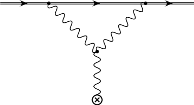
(a) (b)

Figure 2: Diagrams contributing to the background field tadpoles at order $\ell^{-1}\lambda^{2}$. The $\otimes$ denotes an insertion of the background graviton field.

Since the source is at rest, Fig. 2(b) only gives a contribution to the ${\bar{h}}_{00}$ tadpole

$$\mbox{Fig.}~{}\ref{m2}(b)=-{i\over 2}m_{0}\left({r_{s}\over L}\right)^{d-3}\zeta(d-3)\int dt{\bar{h}}_{00}.$$ (41)

Combining these results we find to first order in $\lambda$

$${m\over m_{0}} = 1-{1\over 2}{\hat{\lambda}}$$ (42)

$${\tau L\over m_{0}} = {1\over 2}(d-3){\hat{\lambda}},$$ (43)

where we have defined ${\hat{\lambda}}=\zeta(d-3)\left({r_{s}\over L}\right)^{(d-3)}$. This reproduces the results of hd ; kold .

III.2 Order $\lambda^{2}$

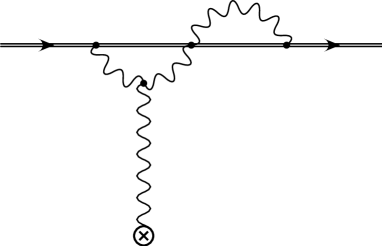
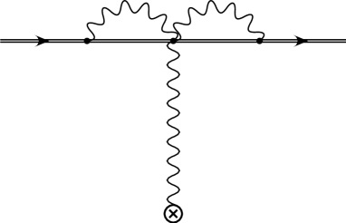
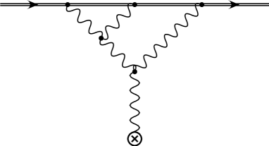
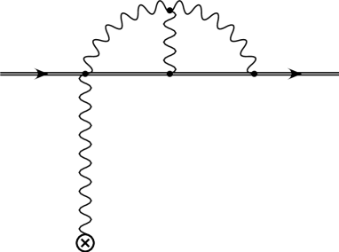
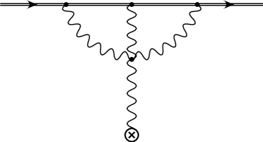
(a) (b) (c) (d) (e) (f)

Figure 3: Diagrams contributing to the background field tadpoles at order $\ell^{-1}\lambda^{3}$. The $\otimes$ denotes an insertion of the background graviton field.

It is convenient to consider separately the corrections to the $\int dt{\bar{h}}_{00}$, $\int dt{\bar{h}}_{zz}$ terms in the effective action. For the $\int dt{\bar{h}}_{zz}$ terms, the diagrams in Fig. 3(a), Fig. 3(c), and Fig. 3(e) do not contribute.

It is straightforward to derive the Feynman rules necessary to calculate the diagrams of Fig. 3. We will simply write down the results of evaluating each diagram. For the $\int dt{\bar{h}}_{00}$ tadpoles in the effective action, one finds that evaluating the diagrams at zero external momentum gives rise to no new integrals: the integration over the internal momenta factorizes into the square of the integrals $I_{0,1}(L)$ of the previous section. The results are

$$\mbox{Fig.}~{}\ref{m3}(a) = -{i\over 2}m_{0}{\hat{\lambda}}^{2}\int dt{\bar{h}}_{00},$$ (44)

$$\mbox{Fig.}~{}\ref{m3}(b) = {3i\over 2}m_{0}{\hat{\lambda}}^{2}\int dt{\bar{h}}_{00},$$ (45)

$$\mbox{Fig.}~{}\ref{m3}(c) = -{3i\over 4}m_{0}{\hat{\lambda}}^{2}\int dt{\bar{h}}_{00},$$ (46)

$$\mbox{Fig.}~{}\ref{m3}(d) = -{i\over 4}{13d-43\over d-3}m_{0}{\hat{\lambda}}^{2}\int dt{\bar{h}}_{00},$$ (47)

$$\mbox{Fig.}~{}\ref{m3}(e) = {3i\over 2}m_{0}{\hat{\lambda}}^{2}\int dt{\bar{h}}_{00},$$ (48)

$$\mbox{Fig.}~{}\ref{m3}(f) = {i\over 4}{5d-19\over d-3}m_{0}{\hat{\lambda}}^{2}\int dt{\bar{h}}_{00}.$$ (49)

For the tadpole terms $\int dt{\bar{h}}_{zz}$, we find from Fig. 3(b)

$$\mbox{Fig.}~{}\ref{m3}(b)={i\over 2}(d-3)m_{0}{\hat{\lambda}}^{2}\int dt{\bar{h}}_{zz}.$$ (50)

The contribution of graphs Fig. 3(d), Fig. 3(f) to the tadpole $\int dt{\bar{h}}_{00}$ does not factorize into the integrals of the form $I_{0,1}(L)$. However their sum does,

$$\mbox{Fig.}~{}\ref{m3}(d)+\mbox{Fig.}~{}\ref{m3}(f)=-{i}m_{0}(d-3){\hat{\lambda}}^{2}\int dt{\bar{h}}_{zz}.$$ (51)

Thus the ${\cal O}(\ell\lambda^{2})$ terms in the effective action are

$$\left.\Gamma[{\bar{h}}]\right|_{\ell\lambda^{2}}=-{1\over 4}m_{0}{\hat{\lambda}}^{2}\int dt{\bar{h}}_{00}-{1\over 2}m_{0}(d-3){\hat{\lambda}}^{2}\int dt{\bar{h}}_{zz}.$$ (52)

IV Thermodynamics

We have found, from the diagrams in Fig. 2 and Fig. 3

$${m\over m_{0}} = 1-{1\over 2}{\hat{\lambda}}+{1\over 2}{\hat{\lambda}}^{2}$$ (53)

$${\tau L\over m_{0}} = {1\over 2}(d-3){\hat{\lambda}}-(d-3){\hat{\lambda}}^{2}$$ (54)

To obtain observables which can be tested against the numerical data of kolnumeric ; kudoh1 ; kudoh2 , we must eliminate the unphysical bare mass parameter $m_{0}$ from these two equations. This gives,

$${2\over d-3}{\tau L\over m}=\zeta(d-3){2G_{N}m\over L^{d-3}}-\zeta^{2}(d-3)\left({2G_{N}m\over L^{d-3}}\right)^{2}+\cdots,$$ (55)

which agrees with the results of 5d when $d=5$.

We may then relate the asymptotic charge to the thermodynamics quantities via Smarr’s relation $(d-3)m=(d-2)TS+\tau L$ (see ref. ho2 ; koltheory ) which, using Eq. (55), gives $TS$ as a function of $m,L$. As $L\rightarrow\infty$ the entropy $S$ simply becomes the entropy of an isolated $d$-dimensional black hole. This scales like the area of the black hole, $S\sim r_{s}^{d-2}\sim m^{{d-2\over d-3}}$. Thus for $\lambda\ll 1$ we expect

$$S=m^{{d-2\over d-3}}f\left(G_{N}m\over L^{d-3}\right).$$ (56)

The function $f(z)$ can be obtained from the relation

$${1\over T}=\left.{\partial S\over\partial M}\right|_{L}$$ (57)

together with the formula for $TS$ that follows from Smarr’s law. We finds

$${S\over S(L\rightarrow\infty)}=1+{1\over 2}\left({d-2\over d-3}\right)\zeta(d-3){2G_{N}m\over L^{d-3}}+{1\over 8}{d-2\over(d-3)^{2}}\zeta^{2}(d-3)\left({2G_{N}m\over L^{d-3}}\right)^{2}+\cdots,$$ (58)

and

$${T\over T(L\rightarrow\infty)}=1-{2d-5\over 2(d-3)}\zeta(d-3){2G_{N}m\over L^{d-3}}+\left[8d^{2}-43d+58\over 8(d-3)^{2}\right]\zeta^{2}(d-3)\left({2G_{N}m\over L^{d-3}}\right)^{2}+\cdots,$$ (59)

where $S(L\rightarrow\infty)$ and $T(L\rightarrow\infty)$ are the entropy and temperature of an uncompactified black hole,

$$S(L\rightarrow\infty) = {2\pi\over(d-2)G_{N}}r^{d-2}_{s},$$ (60)

$$T(L\rightarrow\infty) = {d-3\over 4\pi r_{s}}.$$ (61)

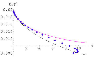
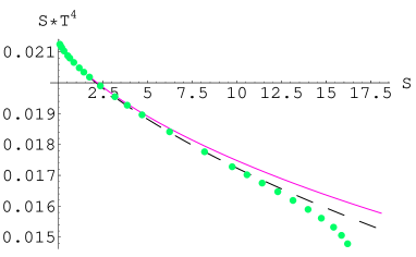
(a) (b)

Figure 4: Comparison of analytic results with the data of refs. kudoh1 ; kudoh2 . (a) compares the $d=5$ results and (b) the $d=6$ results. The dashed lines include only ${\cal O}(\lambda)$ corrections. The solid lines include ${\cal O}(\lambda^{2})$ terms.

We may then compare with the numerical results of Kudoh and Wiseman kudoh1 ; kudoh2 in the special cases of five and six dimensions which are shown in Fig. 4(a) and Fig. 4(b) respectively. The difference between the numerical data and the analytical results grows with $S$, but it is difficult to gauge the relevance of this deviation without some measure of the errors in the numerical computation. As a crude measure of convergence of the perturbative expansion we plot in Fig. 5 the ratio of the ${\cal O}(\lambda^{2})$ to the ${\cal O}(\lambda)$ terms in the series expansion for $ST^{d-2}$ versus $S$.

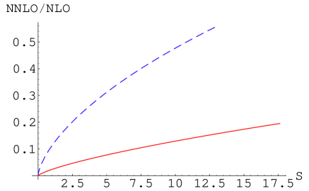
Figure 5: Ratio of ${\cal O}(\lambda^{2})$ to ${\cal O}(\lambda)$ terms in the perturbative expansion of $TS^{d-2}$ versus $S$ for $d=5$ (dashed line) and $d=6$ (solid line).

V Conclusions

In this paper, we have used EFT methods to determine the qualitative structure of the thermodynamics of Kaluza-Klein black holes when their radius is much smaller than the compactification scale. Using the power counting in the EFT, we find that the asymptotic charges $m,\tau$ are related in the regime $v^{2}=G_{N}m/L^{d-2}\ll 1$ by an expansion of the form

$${\tau L\over m}=f_{0}(v^{2})+\sum^{\infty}_{n=1}v^{2\gamma_{n}}f_{n}(v^{2}),$$ (62)

where $f_{n}(v^{2})$ is analytic about zero and $\gamma_{n}=2+4n/(d-3)$. For $n=0$, we find

$$f_{0}(v^{2})={1\over 2}(d-3)\left[\zeta(d-3)v^{2}-\zeta(d-3)^{2}v^{4}+{\cal O}(v^{6})\right],$$ (63)

which agrees with the ${\cal O}(v^{2})$ results of kold in $d$ spacetime dimensions and with the ${\cal O}(v^{4})$ $d=5$ results of 5d calculated in perturbation theory about the full uncompactifed Schwarzschild background. Thus our results indicate that the existing analytical tests of the numerics for $d=5,6$ only probe the thermodynamics of point particles and are not sensitive to the dynamics of the black hole horizon. It would be interesting to repeat the numerical simulations for large dimension where the phase diagram is more sensitive to the structure of the horizon. For instance in $d\geq 8$, the first finite size effect comes in at order $\lambda^{p}$, $2<p<3$, and is distinguishable from terms in the black hole thermodynamics that can be reproduced by a minimal point particle action $-m\int ds$.

Acknowledgments

We thank H. Kudoh and T. Wiseman for making the numerical results of kudoh1 ; kudoh2 available to us, and T. Wiseman for helpful discussions. Y-ZC and WG are supported in part by the Department of Energy under Grant DE-FG02-92ER40704. IZR is supported in part by the Department of Energy under Grants DOE-ER-40682-143 and DEAC02-6CH03000.

References

- (1) R. Gregory and R. Laflamme, “Black strings and -branes are unstable,” Phys. Rev. Lett. 70, 2837 (1993) [arXiv:hep-th/9301052].
- (2) R. Gregory and R. Laflamme, “The Instability of charged black strings and -branes,” Nucl. Phys. B 428, 399 (1994) [arXiv:hep-th/9404071].
- (3) B. Kol, “The phase transition between caged black holes and black strings: A review,” arXiv:hep-th/0411240.
- (4) T. Harmark and N. A. Obers, “Phases of Kaluza-Klein black holes: A brief review,” arXiv:hep-th/0503020.
- (5) G. T. Horowitz and K. Maeda, “Fate of the black string instability,” Phys. Rev. Lett. 87, 131301 (2001) [arXiv:hep-th/0105111].
- (6) S. S. Gubser, “On non-uniform black branes,” Class. Quant. Grav. 19, 4825 (2002) [arXiv:hep-th/0110193].
- (7) O. Aharony, J. Marsano, S. Minwalla and T. Wiseman, “Black hole - black string phase transitions in thermal 1+1 dimensional supersymmetric Yang-Mills theory on a circle,” Class. Quant. Grav. 21, 5169 (2004) [arXiv:hep-th/0406210].
- (8) O. Aharony, J. Marsano, S. Minwalla, K. Papadodimas, M. Van Raamsdonk and T. Wiseman, “The phase structure of low dimensional large gauge theories on tori,” arXiv:hep-th/0508077.
- (9) T. Harmark and N. A. Obers, “Black holes on cylinders,” JHEP 0205, 032 (2002) [arXiv:hep-th/0204047].
- (10) R. C. Myers, “Higher Dimensional Black Holes In Compactified Space-Times,” Phys. Rev. D 35, 455 (1987).
- (11) E. Sorkin, B. Kol and T. Piran, Phys. Rev. D 69, 064032 (2004) [arXiv:hep-th/0310096].
- (12) H. Kudoh and T. Wiseman, “Properties of Kaluza-Klein black holes,” Prog. Theor. Phys. 111, 475 (2004) [arXiv:hep-th/0310104].
- (13) H. Kudoh and T. Wiseman, “Connecting black holes and black strings,” Phys. Rev. Lett. 94, 161102 (2005) [arXiv:hep-th/0409111].
- (14) T. Harmark, Phys. Rev. D 69, 104015 (2004) [arXiv:hep-th/0310259].
- (15) D. Gorbonos and B. Kol, “Matched asymptotic expansion for caged black holes: Regularization of the post-Newtonian order,” Class. Quant. Grav. 22, 3935 (2005) [arXiv:hep-th/0505009].
- (16) D. Karasik, C. Sahabandu, P. Suranyi and L. C. R. Wijewardhana, “Analytic approximation to 5 dimensional black holes with one compact dimension,” Phys. Rev. D 71, 024024 (2005) [arXiv:hep-th/0410078].
- (17) D. Gorbonos and B. Kol,“A dialogue of multipoles: Matched asymptotic expansion for caged black holes,” JHEP 0406, 053 (2004) [arXiv:hep-th/0406002].
- (18) T. Harmark and N. A. Obers, “New phase diagram for black holes and strings on cylinders,” Class. Quant. Grav. 21, 1709 (2004) [arXiv:hep-th/0309116].
- (19) B. Kol, E. Sorkin and T. Piran, “Caged black holes: Black holes in compactified spacetimes. I: Theory,” Phys. Rev. D 69, 064031 (2004) [arXiv:hep-th/0309190].
- (20) W. D. Goldberger and I. Z. Rothstein, “An effective field theory of gravity for extended objects,” arXiv:hep-th/0409156.
- (21) W. D. Goldberger and I. Z. Rothstein, “Dissipative effects in the worldline approach to black hole dynamics,” arXiv:hep-th/0511133.
- (22) R. A. Porto, “Post-Newtonian corrections to the motion of spinning bodies in NRGR,” arXiv:gr-qc/0511061.
- (23) B. DeWitt, in Relativity, Groups and Topology, Proceedings of the Les Houches Summer School of Theoretical Physics, eds. C. DeWitt and B. DeWitt, Gordon and Breach, 1964.
- (24) M. Veltman, in Methods in Field Theory, Proceedings of the Les Houches Summer School, 1975, eds. R. Balian and J. Zinn-Justin, North Holland, 1976.
- (25) H. Kodama and A. Ishibashi, “A master equation for gravitational perturbations of maximally symmetric black holes in higher dimensions,” Prog. Theor. Phys. 110, 701 (2003) [arXiv:hep-th/0305147].
- (26) A. Ishibashi and H. Kodama, “Stability of higher-dimensional Schwarzschild black holes,” Prog. Theor. Phys. 110, 901 (2003) [arXiv:hep-th/0305185].