Abstract

We study a statistical model of random plane partitions. The statistical model has interpretations as five-dimensional $\mathcal{N}=1$ supersymmetric $SU(N)$ Yang-Mills on $\mathbb{R}^{4}\times S^{1}$ and as Kähler gravity on local $SU(N)$ geometry. At the thermodynamic limit a typical plane partition called the limit shape dominates in the statistical model. The limit shape is linked with a hyperelliptic curve, which is a five-dimensional version of the $SU(N)$ Seiberg-Witten curve. Amoebas and the Ronkin functions play intermediary roles between the limit shape and the hyperelliptic curve. In particular, the Ronkin function realizes an integration of thermodynamical density of the main diagonal partitions, along one-dimensional slice of it and thereby is interpreted as the counting function of gauge instantons. The radius of $S^{1}$ can be identified with the inverse temperature of the statistical model. The large radius limit of the five-dimensional Yang-Mills is the low temperature limit of the statistical model, where the statistical model is frozen to a ground state that is associated with the local $SU(N)$ geometry. We also show that the low temperature limit corresponds to a certain degeneration of amoebas and the Ronkin functions known as tropical geometry.

1 Introduction and summary

It is an old idea that spacetime may have more than four dimensions, with extra coordinates being unobservable at available energies. A first possibility arises in the Kaluza-Klein theory. In the Kaluza-Klein approach, gravitation and electromagnetism could be unified in a theory of five-dimensional geometry. The extra dimension makes $S^{1}$ that radius is microscopically small. The Kaluza-Klein like approach has always been one of the most intriguing ideas in physics.

The idea of the Kaluza-Klein theory is utilized in superstring theory [1]. Superstring theory is a candidate for a theory of everything. When superstring theory is completed, all four-dimensional theories, such as standard model and general relativity, can be derived from superstring theory. In superstring theory, strings which are one-dimensional objects play a central role instead of point particles. Each elementary particle corresponds to each vibration mode of string. While it moves in a spacetime, a string sweeps out a two-dimensional surface. So the motion of a string is given by a map from a two-dimensional surface $\Sigma$, called the worldsheet, to a spacetime. In this sense the spacetime is often called the target space. Superstring theory makes sense only in ten spacetime dimensions (at least in perturbative treatments). Is it a pity that the spacetime dimension is not four? We don’t think so. We take the ten-dimensional space to be of the form $M^{4}\times X$, where $M^{4}$ is our four-dimensional Minkowski space and $X$ is a compact six-dimensional space. From the physical viewpoint, the most interesting candidate for $X$ is Calabi-Yau threefolds. We cannot look at $X$ directly, however geometrical natures of $X$ turn up as physical properties in $M^{4}$, such as the gauge symmetry and the matter content. Studying superstring theory on $M^{4}\times X$, one can find that the internal properties of $X$ lead to physical consequences for the observers living in $M^{4}$.

Supersymmetric theories [2] give laboratories to test these ideas. Supersymmetric theories are more tractable than ordinary non-supersymmetric theories, and many of their observables can be computed exactly. Nevertheless, it turns out that these theories exhibit explicit examples of various phenomena in quantum field theories. Then it has become a priority in particle physics to understand better the perturbative and non-perturbative dynamics of supersymmetric theories. $\mathcal{N}=2$ supersymmetric gauge theories have been particularly studied at both perturbative and non-perturbative levels. The extended supersymmetry dramatically simplifies the dynamics of gauge theories. $\mathcal{N}=2$ gauge theories also have an interesting interpretation from the perspective of superstring theories. It is called the geometric engineering [3]. According to the geometric engineering, $\mathcal{N}=2$ supersymmetric gauge theory is realized by the type IIA superstring on a certain Calabi-Yau threefold. Some physical properties in the gauge theory is derived from geometrical natures of the Calabi-Yau threefold. The gauge symmetry is closely related with the ADE singularity in the Calabi-Yau threefold. For example, the $SU(N)$ gauge symmetry is realized by an $A_{N-1}$-type singularity. The geometry which leads to the $SU(N)$ gauge theory is often called the local $SU(N)$ geometry. The geometric engineering connects four-dimensional gauge theories with geometries of internal spaces. This gives an example of the gauge/gravity correspondence. It goes without saying that the most important principle in physics is gauge theory and general relativity. The duality between these two theories is an interesting research area in particle physics. AdS/CFT correspondence [4, 5] is one of the most remarkable examples of this duality.

In the last few years, there has been great progress in both superstring theories and supersymmetric gauge theories. The exact low-energy dynamics of $\mathcal{N}=2$ supersymmetric gauge theories has been revealed by Seiberg and Witten [6]. They have evaluated exact low-energy effective actions of $\mathcal{N}=2$ theories using the holomorphy and a version of the electromagnetic duality. The low-energy effective theory obtained by them led to numerous achievements in understanding of the non-perturbative dynamics of gauge theories. Their derivation is elegant but follows in a somewhat indirect way. Recently, Nekrasov and Okounkov have calculated exact low-energy effective actions in a more direct way [7, 8]. They have evaluated the path integrals of $\mathcal{N}=2$ supersymmetric gauge theories and give exact formulae for both perturbative and non-perturbative dynamics. The Seiberg-Witten solutions emerges through statistical models of random partitions. Also, Nakajima and Yoshioka derived independently the Seiberg-Witten solutions by taking the algebraic geometry viewpoint [9].

Recent progress in superstring theories is attributed to understanding of topological strings. Topological string is a simplified model of superstring theories, first proposed by Witten [10], which capture topological information of the target space. In the past ten years or so, it has turned out that topological strings have an enormous amount of applications. Their structure is complicated enough to relate them to physically interesting theories, yet simple enough to be able to obtain exact results. There are two different variations in topological strings, the A-model and the B-model. We are interested in the A-model. Topological A-model string amplitudes for a certain class of geometries can be computed using a diagrammatical method, called the topological vertex [11, 12]. One of the most interesting applications of topological strings is the geometric engineering. The topological vertex allows us to evaluate the topological string amplitude for the local $SU(N)$ geometry. The result of topological strings actually reproduces Nekrasov’s formula for $\mathcal{N}=2$ $SU(N)$ gauge theory [13, 14].

The method of the topological vertex yields an unanticipated but very exciting connection between the topological string and a statistical model of random plane partitions [15]. This connection has a surprising interpretation as quantum gravity. Quantum theory of gravity is the holy grail of physics. In quantum gravity spacetime undergoes quantum fluctuations, which cause wild fluctuations of the geometry and the topology of spacetime. These quantum fluctuations make spacetime foamy at short length scales [16]. This idea is very exciting, but we haven’t made a precise understanding of quantum gravity yet. It is believed that superstring theory gives rise to quantum gravity on the target space. The topological string can also generate a quantum gravitational theory. It is expected that the classical part of this target space field theory is the Kähler gravity [17]. The classical theory seems to receive quantum deformations caused by string propagation. It is conjectured in [18] that the statistical model of random plane partitions is nothing but the quantum Kähler gravity. The gravitational path integral involving fluctuations of geometry and topology on the target space is interpreted as the statistical sum in the plane partition model. Namely, each plane partition corresponds to a geometry of the target space. Then the plane partition model can give a precise description of the target space quantum gravity.

In this article, we investigate a certain model of random plane partitions and its physical applications. Our motivation is to understand the relation between superstring theories and gauge theories, and clarify the gauge/gravity correspondence between the gauge theories and the internal space gravities. We think that the well-defined statistical model gives a useful tool to study these relations. Besides, our statistical model would be a good laboratory for studying quantum gravity.

A plane partition $\pi$ is an array of non-negative integers

$$\begin{array}[]{cccc}\pi_{11}&\pi_{12}&\pi_{13}&\cdots\\ \pi_{21}&\pi_{22}&\pi_{23}&\cdots\\ \pi_{31}&\pi_{32}&\pi_{33}&\cdots\\ \vdots&\vdots&\vdots&{}\hfil\end{array}$$ (1.5)

satisfying $\pi_{ij}\geq\pi_{i+1j}$ and $\pi_{ij}\geq\pi_{ij+1}$ for all $i,j\geq 1$. It is identified with the three-dimensional Young diagram as depicted in Figure 1-(a). The three-dimensional diagram $\pi$ is a set of unit cubes such that $\pi_{ij}$ cubes are stacked vertically on each $(i,j)$-element of $\pi$. The diagram is also regarded as a sequence of partitions $\pi(m)$, where $m\in\mathbb{Z}$. A partition is identified with the (two-dimensional) Young diagram. See Figure 1-(b).

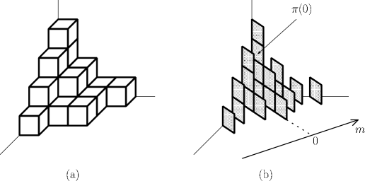
Figure 1: The three-dimensional Young diagram (a) and the corresponding sequence of partitions (the two-dimensional Young diagrams) (b).

Among the series of partitions, a partition at the main diagonal $m=0$, denoted by $\pi(0)$, will be called the main diagonal partition of $\pi$ and play an central role in our argument. We consider the following model of random plane partitions.

$$Z(q,Q)=\sum_{\pi}\,q^{|\pi|}\,Q^{|\pi(0)|},$$ (1.6)

where $q$ and $Q$ are indeterminates. $|\pi|$ and $|\pi(0)|$ denote respectively the total numbers of cubes and boxes of the corresponding diagrams. The model with $Q=1$ is well-known [19]. The authors of [15] investigated the $Q=1$ model and proposed a connection between the model and topological strings. Our plane partition model contains a new parameter $Q$. By an identification of $q$ and $Q$ with the relevant string theory parameters, the partition function (1.6) can be converted into topological A-model string amplitude on a certain Calabi-Yau threefold. We can also retrieve Nekrasov’s formulae for five-dimensional $\mathcal{N}=1$ supersymmetric Yang-Mills theories from the partition function [20].

The above model has an interpretation as random partitions or the $q$-deformation. It can be seen by rewriting the partition function as

$$Z(q,Q)=\sum_{\lambda}\,Q^{|\lambda|}\,\Bigl{(}\sum_{\pi(0)=\lambda}\,q^{|\pi|}\Bigr{)},$$ (1.7)

where the summation over plane partitions in (1.6) are divided into two branches. The partitions $\lambda$ are thought as the ensemble of the model by summing first over the plane partitions whose main diagonal partitions are $\lambda$.

It is known [21] that a partition $\lambda$ has an alternative realization in terms of $N$ charged partitions $\{(\lambda^{(r)},p_{r})\}_{r=1}^{N}$. The charges $p_{r}$ are subject to the condition $\sum_{r=1}^{N}p_{r}=0$. Among partitions, these coming from the charged empty partitions $\{(\emptyset,p_{r})\}_{r=1}^{N}$ turn to play special roles. They are called $N$ cores. The above realization allows us to read the summation over partitions in (1.7) by means of $N$ charged partitions. Regarding the model as the $q$-deformed random partitions, we will factor the partition function into

$$Z(q,Q) = \sum_{\{p_{r}\}}\,Z^{pert}_{SU(N)}(\{p_{r}\};q,Q)\,\sum_{\{\lambda^{(r)}\}}Z^{inst}_{SU(N)}(\{\lambda^{(r)}\},\{p_{r}\};q,Q)$$ (1.8)

$$= \sum_{\{p_{r}\}}\,Z_{SU(N)}(\{p_{r}\};q,Q)\,.$$

In the first line we write the Boltzmann weight for the $N$ core, that is read from (1.7), by $Z^{pert}_{SU(N)}(\{p_{r}\};q,Q)$. In the second line we have included the summation over partitions $\lambda^{(r)}$ implicitly in $Z_{SU(N)}(\{p_{r}\};q,Q)$. This factorization turns out useful to find out the gauge theoretical interpretations. The relevant field theory parameters are $a_{r},\Lambda$ and $R$, where $a_{r}$ are the vacuum expectation values of the adjoint scalar in the vector multiplet and $\Lambda$ is the scale parameter of the underlying four-dimensional theory. $R$ is the radius of $S^{1}$ in the fifth dimension. We identify these parameters with $q,Q$ and $p_{r}$ in (1.8) as follows.

$$q=e^{-\frac{R}{N}\hbar},~{}~{}~{}~{}Q=(R\Lambda)^{2},~{}~{}~{}~{}p_{r}=a_{r}/\hbar\,.$$ (1.9)

The parameter $\hbar$ is often identified with the string coupling constant $g_{st}$. The above identification leads [20] to

$$Z_{SU(N)}(\{p_{r}\};q,Q)=Z_{\,5d\,\mbox{\scriptsize SYM}}(\{a_{r}\};\,\Lambda,R,\hbar),$$ (1.10)

where the RHS is the exact partition function [8] for five-dimensional $\mathcal{N}=1$ supersymmetric $SU(N)$ Yang-Mills with the Chern-Simons term. The five-dimensional theory is living on $\mathbb{R}^{4}\times S^{1}$. The Chern-Simons coupling constant $c_{cs}$ is quantized to $N$. Actually, the identification (1.9) shows that the perturbative part and the instanton part of the exact partition function for the gauge theory are given by $Z_{SU(N)}^{pert}$ and $\sum_{\{\lambda^{(r)}\}}Z_{SU(N)}^{inst}$ respectively.

The gauge theory prepotential is revealed from the exact partition function by taking the semiclassical limit, that is, the $\hbar\rightarrow 0$ limit. This corresponds to the thermodynamic limit of the statistical model. At the thermodynamic limit, the typical volume of the three-dimensional Young diagrams or plane partitions is $\sim\hbar^{-3}$ and the variance of the volume is $\sim\hbar^{-4}$. Rescaling in all directions by a factor $\hbar$, the typical three-dimensional Young diagrams approach a smooth limit shape which is a two-dimensional surface in the octant. For the $Q=1$ model, such a limit was considered in [22] and one can obtain the limit shape as in Figure 2.

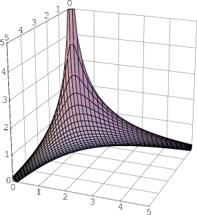
Figure 2: The limit shape of the simple model $Z(q,Q=1)=\sum_{\pi}q^{|\pi|}$.

In the Seiberg-Witten approach, hyperelliptic curves known as the Seiberg-Witten curves play an important role. Given a gauge group and matter content, the potential of the $\mathcal{N}=2$ supersymmetric gauge theory has flat directions, so that the $\mathcal{N}=2$ theory has a space of physically inequivalent vacua. This space is often called the vacuum moduli space. The vacuum moduli space can be identified with the moduli space of the Riemann surfaces. For example, each vacua of the $SU(N)$ Yang-Mills theory corresponds to a hyperelliptic curve with genus $N-1$ [23].

The connection between the plane partition model and the $SU(N)$ Yang-Mills suggests a relation between the limit shape and the hyperelliptic curve. In order to find out the relation, we focus our attention on the main diagonal partitions and consider the thermodynamic limit of each component that appears in the factorization (1.8) of the plane partition model. We introduce a density $\rho(x|\lambda;p)$ of a charged partition $(\lambda,p)$. To obtain a finite limit shape we must scale partitions in a certain manner at the thermodynamic limit. Thereby the density of a partition $\lambda$ is scaled to $\rho(u|\lambda)$. The asymptotic form of the Boltzmann weight of the plane partition model is expressed as an energy functional of the scaled density.

$$\log\bigg{(}Q^{|\lambda|}\sum_{\pi(0)=\lambda}q^{|\pi|}\bigg{)}=-\frac{1}{\hbar^{2}}\big{\{}E[\rho(\cdot|\lambda)]+O(\hbar)\big{\}}$$ (1.11)

The minimizer of the energy functional gives the typical shape of the main diagonal partitions at the thermodynamic limit. The minimizer that realizes the thermodynamic limit of the component must be found from configurations that are expressible in terms of $N$ charged partitions with the fixed charges.

The variational problem of the energy functional can be solved by using the standard argument [24]. The solution $\rho_{\star}^{SU(N)}$ turns to be realized using data of the hyperelliptic curve.

$$y+y^{-1}=\frac{1}{(R\Lambda)^{N}}\prod_{r=1}^{N}(e^{Rz}-\beta_{r}),$$ (1.12)

where $\beta_{r}$ are real positive numbers determined by the charges. This curve is thought to be a five-dimensional version of the $SU(N)$ Seiberg-Witten curve and reduces to the Seiberg-Witten curve of four-dimensional $\mathcal{N}=2$ $SU(N)$ Yang-Mills at the limit $R\to 0$.

The more direct link between the limit shape and the Seiberg-Witten curve can be revealed. To this end, we introduce a new object called an amoeba [25, 26]. The amoeba of a Laurent polynomial $f(x,y)$ is, by definition, the image in $\mathbb{R}^{2}$ of the zero locus of $f(x,y)$ under the simple mapping $\mathrm{Log}$ that takes each coordinate to the logarithm of its modulus. We put $(u,v)=\mathrm{Log}(x,y)$ to be coordinates of $\mathbb{R}^{2}$ where amoebas live. The most important tool to study amoebas is the remarkable Ronkin function $N_{f}(u,v)$, which is a convex function over $\mathbb{R}^{2}$. It has been verified in [22] that the limit shape of the statistical model with $Q=1$ is expressed by the Ronkin function of an amoeba. We give pieces of evidence for the relation in our statistical model. For the $SU(N)$ gauge theory, we employ the polynomial.

$$f_{SU(N)}(x,y)=\prod_{r=1}^{N}(x-\beta_{r})-(R\Lambda)^{N}(y+y^{-1})\,.$$ (1.13)

The curve $f_{SU(N)}(e^{Rz},y)=0$ is the hyperelliptic curve (1.12). We focus our attention on the Ronkin function over the $u$-axis. We will verify the following relation between the Ronkin function and the minimizer.

$$N_{f_{SU(N)}}(u,v=0)=N\int_{-\infty}^{u}d\underline{u}\,\,\rho_{\star}^{SU(N)}(\underline{u})\hskip 5.69054pt+\,\mbox{const}.$$ (1.14)

Since the minimizer expresses the gradient of the limit shape at the main diagonal, the above relation shows that the Ronkin function of $f_{SU(N)}$ is identical with the limit shape of plane partitions at least over the main diagonal. In terms of the internal space geometry, the limit shape corresponds to a low-energy solution of the Kähler gravity. On the other hand, the Seiberg-Witten curve describes the non-perturbative vacuum structure of the $\mathcal{N}=2$ gauge theory. Therefore the above connection gives the full gauge/gravity correspondence. The low-energy geometry contains large quantum fluctuations from the local $SU(N)$ geometry. These quantum fluctuations would correspond to the instanton correction in the gauge theory.

One of the most interesting phenomena in superstring theory is the mirror symmetry [27, 28]. The mirror symmetry is a T-duality, in which two very different internal spaces give rise to equivalent superstring theory. In terms of topological strings, the mirror symmetry states that the topological A-model on a Calabi-Yau threefold is equivalent to the B-model on a mirror Calabi-Yau threefold. For the local $SU(N)$ geometry, the mirror Calabi-Yau threefold is specified by the hyperelliptic curve $f_{SU(N)}(x,y)=0$ [29]. Therefore, the above relation is also a manifestation of the mirror symmetry.

Ronkin’s functions appear in the dimer problem of bipartite lattice graphs [30, 31]. A dimer is a dumb-bell shaped molecule that occupies two adjacent lattice sites, and the dimer problem is to determine the number of ways of covering the lattice with dimers so that all sites are occupied and no two dimers overlap. When dimers are magnetically charged, the free energy per area is given by a Ronkin’s function at the thermodynamic limit, where the coordinates $(u,v)$ represent constant magnetic field $B$ [32]. The connection with quiver gauge theories has been argued in [33].

The parameter $R$ is identified with the radius of $S^{1}$ in the fifth dimension of the gauge theories. In the plane partition model, if one keeps $R\Lambda$ fixed, this parameter is interpreted as the inverse temperature, that is, $R=1/T$, where $T$ denotes the temperature. Therefore the large radius limit of the gauge theories corresponds to the low temperature limit of the statistical models. As the temperature approaches to zero, the statistical models get to freeze to the ground states. Each ground state is a specific plane partition that is determined by the $N$ core at the main diagonal. Crystal is the complement of the ground state in the octant. It has an interpretation as the gravitational quantum foam of the local $SU(N)$ geometry [34]. The crystal also has an interpretation in amoebas. We will show that the low temperature limit $R\rightarrow\infty$ corresponds to a certain degeneration of the amoeba and the Ronkin function known as tropical geometry [35, 36, 37]. For instance, facet of the crystal is described by a piecewise linear function which is the degeneration of the Ronkin function $N_{f_{SU(N)}}(u,v)$ at the limit $R\rightarrow\infty$.

This article is organized as follows. After introducing amoebas briefly in section 2, we associate amoebas with local Calabi-Yau geometries that geometric engineer supersymmetric gauge theories having eight supercharges, and investigate the amoebas and their Ronkin functions. In section 3 we study the thermodynamic limit of the plane partition model. The relation between the limit shapes and the Ronkin functions is shown. In section 4 we describe degenerations of the amoebas and the Ronkin functions, and relate the degenerations with crystals that are realized at the low temperature limit or the large radius limit.

2 Amoebas from local Calabi-Yau geometries

We associate amoebas with local Calabi-Yau geometries that geometric engineer [3] supersymmetric gauge theories having eight supercharges. The amoebas live in $\mathbb{R}^{2}$. We investigate the Ronkin functions for these amoebas. The Ronkin function is a convex function that is strictly convex over an amoeba and piecewise linear over the amoeba complement. We start this section with an introduction to the notion of amoebas [25] and related objects.

2.1 What is Amoeba ?

Let $f(x,y)=\sum_{i,j\in\mathbb{Z}}a_{ij}x^{i}y^{j}$ be a Laurent polynomial with only a finite number of the $a_{ij}$’s being non-zero. Let $V_{f}$ be the zero locus of the polynomial in $(\mathbb{C}^{*})^{2}$, that is,

$$V_{f}=\Bigl{\{}\left.(x,y)\in(\mathbb{C}^{*})^{2}\,\right|\,\,f(x,y)=0\Bigr{\}}\,.$$ (2.1)

This $V_{f}$ is a punctured Riemann surface. Define the logarithmic map by

$$\begin{array}[]{cclcl}\mathrm{Log}&:&(\mathbb{C}^{*})^{2}&\longrightarrow&\mathbb{R}^{2}\\[2.84526pt] &&(x,\,y)&\longmapsto&(\,\log|x|,\,\log|y|\,)\,.\end{array}$$ (2.4)

The amoeba of $f$ is the image of $V_{f}$.

$$\mathcal{A}_{f}=\mathrm{Log}(V_{f}).$$ (2.5)

The amoeba will typically be a subset of $\mathbb{R}^{2}$ with tentacle-like asymptotes going off to infinity and separating the complement ${}^{c}\mathcal{A}_{f}=\mathbb{R}^{2}\backslash\mathcal{A}_{f}$ into some connected components. Every connected component of the amoeba complement is a convex domain in $\mathbb{R}^{2}$. Simple examples of amoebas are shown in Figure 3.

(a)

(b)

Figure 3: The amoebas of $(a)~{}1+x+y$ and $(b)~{}5+x+x^{-1}-y-y^{-1}$.

One of the main tools to study amoebas is the Ronkin function [26]. We now take $(u,v)$ to be Log$(x,y)$, coordinates on $\mathbb{R}^{2}$ where amoebas live. The Ronkin function is defined by the integral

$$N_{f}(u,v)=\frac{1}{(2\pi i)^{2}}\int_{\scriptstyle|x|=e^{u}\atop\scriptstyle|y|=e^{v}}\frac{dx}{x}\frac{dx}{y}\,\log|f(x,y)|\,\,.$$ (2.6)

The above integrations are over the preimage of a point $(u,v)\in\mathbb{R}^{2}$ under the logarithmic map (2.4). It is clear that the integrand is singular in the amoeba. But the Ronkin function takes real finite values even over there. In fact, $N_{f}$ is a convex function which is strictly convex over $\mathcal{A}_{f}$ and linear over each connected component of ${}^{c}\mathcal{A}_{f}$. This particularly means that the gradient $\nabla N_{f}$ has a definite value over each connected component of ${}^{c}\mathcal{A}_{f}$. As an example, the Ronkin function of $1+x+y$ is plotted in Figure 4.

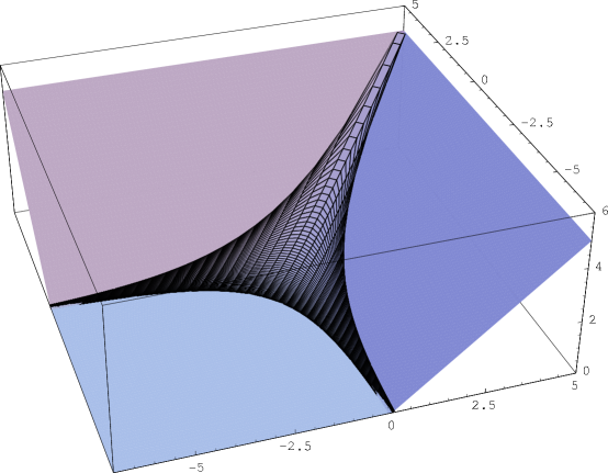
Figure 4: The Ronkin function of $1+x+y$.

The amoeba and the Ronkin function reflect structure of the Newton polygon of the Laurent polynomial. The Newton polygon of $f$ is the minimal convex polygon which contains all points $(i,j)\in\mathbb{Z}^{2}$ corresponding to monomials in the polynomial.

$$\Delta_{f}=\mathrm{convex\ hull\ of}\,\,\bigl{\{}(i,j)\in\mathbb{Z}^{2}\,|\,a_{i,j}\neq 0\bigr{\}}.$$ (2.7)

The Newton polygons of $1+x+y$ and $5+x+x^{-1}-y-y^{-1}$ can be found in Figure 5.

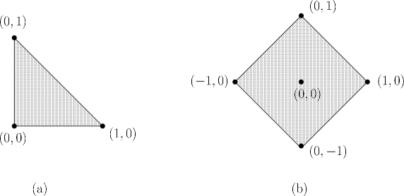
Figure 5: The Newton polygons of $(a)~{}1+x+y$ and $(b)~{}5+x+x^{-1}-y-y^{-1}$.

Figure 6: The spines of the amoebas in Figure 3

Over each connected component $E$ of the amoeba complement ${}^{c}\mathcal{A}_{f}$, the gradient $\nabla N_{f}$ takes value in a integer lattice point of the Newton polygon [26].

$$\bigl{.}\nabla N_{f}\,\bigr{|}_{E}\,\in\Delta_{f}\cap\mathbb{Z}^{2}\,.$$ (2.8)

This gives an upper bound to the number of connected components of ${}^{c}\mathcal{A}_{f}$. The connected components are always less than the lattice points of the Newton polygon. The symbol $E_{(i,j)}$ will be used to denote the connected component over which the gradient $\nabla N_{f}$ equals to $(i,j)$. For almost all the polynomials considered in this paper, the upper bound is attained, that is, the amoeba complement has the same number of the connected components as the lattice points of the Newton polygon. For such a polynomial $f$, we have

$${}^{c}\mathcal{A}_{f}=\bigsqcup_{(i,j)\in\Delta_{f}\cap\mathbb{Z}^{2}}E_{(i,j)}\,.$$ (2.9)

The Ronkin function is piecewise linear over the amoeba complement ${}^{c}\mathcal{A}_{f}$. For each connected component $E$ of ${}^{c}\mathcal{A}_{f}$, let $N_{E}$ be the linear extension of $N_{f}|_{E}$ to $\mathbb{R}^{2}$. When $E=E_{(i,j)}$, we have

$$N_{E_{(i,j)}}(u,v)=c_{(i,j)}+\langle(u,v),(i,j)\rangle\,,$$ (2.10)

where the symbol $\langle\,,\,\rangle$ denotes the standard inner product on $\mathbb{R}^{2}$, that is, $\langle(u,v),(i,j)\rangle=iu+jv$. If the above $(i,j)$ is a vertex of $\Delta_{f}$, the constant $c_{(i,j)}$ is computed and simply becomes $c_{(i,j)}=\Re(\ln a_{i,j})$. According to [26], we introduce a piecewise linear function $S_{f}$ over $\mathbb{R}^{2}$ by

$$S_{f}(u,v)=\max_{E}N_{E}(u,v)\,.$$ (2.11)

Taking account of the convexity of the Ronkin function, it follows

$$N_{f}(u,v)\geq S_{f}(u,v)$$ (2.12)

for any $(u,v)\in\mathbb{R}^{2}$. The equality holds over the amoeba complement ${}^{c}\mathcal{A}_{f}$. So this $S_{f}$ is a piecewise linear function which approximates the Ronkin function by putting sharp corners in it.

The piecewise linear function $S_{f}$ allows us to define the spine of the amoeba $\mathcal{A}_{f}$. The spine $\mathcal{S}$ is the corner set of $S_{f}$, that is, the set of $(u,v)$ where $S_{f}(u,v)$ is not smooth. The spines of the amoebas in Figure 3 are drawn in Figure 6. Note that $\mathcal{S}\subset\mathcal{A}_{f}$. We can regard the spine $\mathcal{S}$ as the 1-skeleton of the convex which is dual to a certain triangular subdivision of the Newton polygon $\Delta_{f}$.

2.2 Amoeba and the Ronkin function for $U(1)$ theory

Geometric engineering [3] dictates that local geometries realize supersymmetric gauge theories. The topological vertex countings [11, 12] of the topological A-model string partition functions on local geometries, which involve from the worldsheet viewpoint sums over holomorphic maps to the target spaces, support [13, 14] the idea. The local geometries are noncompact toric Calabi-Yau threefolds. If a space is toric, many basic and essential characteristics of the space are neatly coded and easily deciphered from analysis of the corresponding lattices. As for the local geometries, the data of the space are retrieved from a two-dimensional polygon. We will regard the polygon as a Newton polygon. Thereby we will define the polynomial for each local geometry.

We first examine an amoeba for the local geometry relevant to the abelian gauge theory. In terms of topological strings, this arises from the topological A-model string on $\mathcal{O}\oplus\mathcal{O}(-2)\to\mathbb{P}^{1}$. The toric polygon of this geometry is drawn in Figure 7.

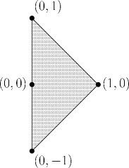
Figure 7: The Newton polygon for U(1) theory.

We employ the following Laurent polynomial.

$$f_{U(1)}(x,y)=x-\beta-R\Lambda\bigl{(}y+y^{-1}\bigr{)}.$$ (2.13)

The parameters $\beta$, $R$ and $\Lambda$ in the above are assumed to be real positive numbers. In particular, we consider the case of $\beta>2R\Lambda$. In the field theory language, $R$ is the radius of $S^{1}$ in the fifth dimension and $\Lambda$ denotes the scale parameter of the underlying four-dimensional theory. It is clear that the Newton polygon of this $f_{U(1)}$ is the polygon in Figure 7.

We will rescale amoebas by $1/R$. This is achieved by using the following rescaled coordinates $(u,v)$ rather than the original ones.

$$(u,v)=\frac{1}{R}\,\mathrm{Log}(x,y)=\bigl{(}\,\frac{1}{R}\log|x|,\,\frac{1}{R}\log|y|\,\bigr{)}.$$ (2.14)

To accord with this, we also rescale the Ronkin functions by $1/R$. In the rest of this paper, we describe amoebas by using the above coordinates, and call the rescaled Ronkin functions simply as the Ronkin functions.

Figure 8: The zero locus $V_{f_{U(1)}}$.

Let us now look at the amoeba of $f_{U(1)}$. The zero locus $V_{f_{U(1)}}$ in $(\mathbb{C}^{*})^{2}$ is a four-punctured sphere. If one regards $\mathbb{C}^{*}$ an infinite cylinder, it is a double covering of the cylinder (Figure 8). The amoeba $\mathcal{A}_{f_{U(1)}}$ is the image $\mathrm{Log}(V_{f_{U(1)}})$. Thanks to the condition $\beta>2R\Lambda$, this becomes a subset of $\mathbb{R}^{2}$ described by the following inequalities.

$$|\beta-2R\Lambda\cosh Rv|\leq e^{Ru}\leq\beta+2R\Lambda\cosh Rv\,.$$ (2.15)

The amoeba is depicted in Figure 9.

Figure 9: The amoeba of $f_{U(1)}$.

The amoeba spreads four tentacles. These tentacles asymptote to the following straight lines and extend to the infinities.

$$v=\pm u\,,\hskip 28.45274ptv=\pm\frac{1}{R}\log\left\{\frac{\beta}{2R\Lambda}+\sqrt{\bigl{(}\frac{\beta}{2R\Lambda}\bigr{)}^{2}-1}\right\}\,.$$ (2.16)

They separate the amoeba complement ${}^{c}\mathcal{A}_{f_{U(1)}}$ into four connected components. The number of connected components agrees with the number of integer lattice points of the Newton polygon.

Taking account of the above rescaling, the Ronkin function $N_{f_{U(1)}}$ is given by

$$N_{f_{U(1)}}(u,v)=\frac{1}{R}\,\frac{1}{(2\pi i)^{2}}\int_{\scriptstyle|x|=e^{Ru}\atop\scriptstyle|y|=e^{Rv}}\frac{dx}{x}\frac{dy}{y}\,\log\left|f_{U(1)}(x,y)\right|\,.$$ (2.17)

Regardless of the simple appearance, it is serious to carry out the above integrations. However, the gradient $\nabla N_{f_{U(1)}}$ becomes tractable since we have

$$\frac{\partial N_{f_{U(1)}}}{\partial u} = \frac{1}{(2\pi i)^{2}}\int_{\scriptstyle|y|=e^{Rv}}\frac{dy}{y}\int_{\scriptstyle|x|=e^{Ru}}\frac{dx}{x-\beta-R\Lambda(y+y^{-1})}\,,$$ (2.18)

$$\frac{\partial N_{f_{U(1)}}}{\partial v} = \frac{1}{(2\pi i)^{2}}\int_{\scriptstyle|x|=e^{Ru}}\frac{dx}{x}\int_{\scriptstyle|y|=e^{Rv}}\frac{d(y+y^{-1})}{R\Lambda(y+y^{-1})-x+\beta}\,.$$ (2.19)

In the double integral (2.18), we can find the following residue integral.

$$\frac{1}{2\pi i}\int_{|x|=e^{Ru}}\frac{dx}{x-\beta-R\Lambda(y+y^{-1})}=\left\{\begin{array}[]{cc}1&\hskip 14.22636pt\mbox{if}~{}~{}~{}|\beta+R\Lambda(y+y^{-1})|\leq e^{Ru}\,,\\[8.53581pt] 0&\mbox{otherwise}.\end{array}\right.$$ (2.22)

The integral takes value $1$ or $0$. If one puts $|y|=e^{Rv}$, the value depends on whether $\theta_{y}=\arg y$ satisfies a certain condition or not, as seen from (2.22). This means that the residue integral is a truth function of the condition on $\theta_{y}$. The $y$-integration in (2.18) gives a simple integration over $\theta_{y}$. We thus interpret $\partial_{u}N_{f_{U(1)}}$ as an integration of the truth function over $\theta_{y}$. The similar interpretation is also possible for $\partial_{v}N_{f_{U(1)}}$ by using (2.19).

Over each connected component of the amoeba complement, the gradient $\nabla N_{f_{U(1)}}$ takes value in an integer lattice point of the Newton polygon. It may be helpful to see how this happens by using the above interpretation. As an example, let us consider the connected component $E$ that is described by the inequality $e^{Ru}>\beta+2R\Lambda\cosh Rv$. We have $|x|>|\beta+R\Lambda(y+y^{-1})|$ for $\forall\,(x,y)\in\mathrm{Log}^{-1}(E)$. This means that the residue integral (2.22) equals to $1$ and we obtain $\partial_{u}N_{f_{U(1)}}=1$ on this connected component. Computation of $\partial_{v}N_{f_{U(1)}}$ goes as well. Thereby we obtain $\nabla N_{f_{U(1)}}=(1,0)$. The connected component $E$ is $E_{(1,0)}$. The other three connected components are $E_{(0,0)}$ and $E_{(0,\pm 1)}$, where the gradient $\nabla N_{f_{U(1)}}$ takes $\alpha$ on each $E_{\alpha}$. Over the amoeba complement the Ronkin function becomes the following piecewise linear function.

$$\Bigl{.}N_{f_{U(1)}}(u,v)\Bigr{|}_{{}^{c}\mathcal{A}_{f_{U(1)}}}=\max_{\alpha=(1,0),(0,\pm 1),(0,0)}\Bigl{(}c_{\alpha}+\langle(u,v),\alpha\rangle\Bigr{)}\,,$$ (2.23)

where the constants $c_{\alpha}$ are

$$c_{(1,0)}=0\,,\hskip 28.45274ptc_{(0,\pm 1)}=\frac{1}{R}\log R\Lambda\,,$$

$$c_{(0,0)}=\frac{1}{R}\log\Bigl{\{}R\Lambda\Bigl{(}\frac{\beta}{R\Lambda}+\sqrt{\bigl{(}\frac{\beta}{2R\Lambda}\bigr{)}^{2}-1}\Bigr{)}\Bigr{\}}\,.$$ (2.24)

We examine the Ronkin function over the amoeba. In particular, we focus on the section of the amoeba along the $u$-axis. In the next section we will see that the Ronkin functions over the $u$-axis relate with instanton countings of gauge theories. The section of the amoeba becomes a segment $I=[\frac{1}{R}\log\beta^{-},\frac{1}{R}\log\beta^{+}]$, where we put $\beta^{\pm}=\beta\pm 2R\Lambda$. Thanks to the condition $\beta>2R\Lambda$, this segment has a finite length. It is convenient to call the segment the band and the complement of it the gap.

Band $$: \ I=\left[\frac{1}{R}\log\beta^{-},\frac{1}{R}\log\beta^{+}\right]\,.$$ (2.25)

Gap $$: \ \mathbb{R}\setminus I\,.$$ (2.26)

The residue integral (2.22) over the gap takes the definite values irrespective of $\theta_{y}$. It always gives $0$ for $u<\frac{1}{R}\log\beta^{-}$ and $1$ for $u>\frac{1}{R}\log\beta^{+}$. On the other hand, when $u$ is in the band, the residue integral takes value $1$ only if $\theta_{y}$ satisfies the inequality.

$$\cos\theta_{y}\leq\frac{e^{Ru}-\beta}{2R\Lambda}\,.$$ (2.27)

Otherwise it gives $0$. Therefore we obtain

$$\frac{\partial N_{f_{U(1)}}}{\partial u}\bigg{|}_{I} = \frac{1}{2\pi}\int_{\cos\theta_{y}\leq\frac{e^{Ru}-\beta}{2R\Lambda}}d\theta_{y}\cdot 1$$ (2.28)

$$= 1+\ \frac{1}{\pi}\arccos\left(\frac{e^{Ru}-\beta}{2R\Lambda}\right)\,,$$

where the branch of the arccosine is fixed by choosing $\arccos(0)=-\pi/2$. To summarize, the gradient of the Ronkin function along the $u$-axis becomes

$$\frac{\partial N_{f_{U(1)}}}{\partial u}\bigg{|}_{v=0}=\left\{\begin{array}[]{lc}0\,,&~{}~{}u<\frac{1}{R}\log\beta^{-}\\[5.69054pt] 1+\frac{1}{\pi}\arccos\left(\frac{e^{Ru}-\beta}{2R\Lambda}\right)\,,&~{}~{}u\in I\\[5.69054pt] 1\,,&~{}~{}\frac{1}{R}\log\beta^{+}<u\,.\end{array}\right.$$ (2.32)

By using this, we plot the Ronkin function over the $u$-axis in Figure 10. For this particular case, our computation is not limited on the $u$-axis and can be done over $\mathbb{R}^{2}$. We plot the Ronkin function over $\mathbb{R}^{2}$ in Figure 11.

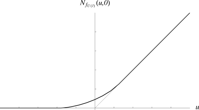
Figure 10: The Ronkin function of $f_{U(1)}$ over the $u$-axis.

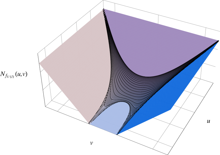
Figure 11: The Ronkin function of $f_{U(1)}$.

The expression (2.32) is arranged by using the terminology of complex geometry. The zero locus $V_{f_{U(1)}}$ is a complex curve in $(\mathbb{C}^{*})^{2}$. It can be written as

$$y+y^{-1}=\frac{1}{R\Lambda}\bigl{(}e^{Rz}-\beta\bigr{)}\,,$$ (2.33)

where $z=u+i\theta/R$ is a cylindrical coordinate of $\mathbb{C}^{*}$. The curve is a double cover of the $\mathbb{C}^{*}$. The branch points locate at two ends of the band $I$. The holomorphic function $y$ has a cut along the band on the Riemann sheet and takes values at the unit circle there. In particular, it is $\pm 1$ at the branch points. Using $y$, we can rewrite (2.32) as follows.

$$\frac{\partial N_{f_{U(1)}}}{\partial u}\bigg{|}_{v=0}=\Re\Bigl{(}1+\frac{1}{\pi i}\log y(u-i0)\Bigr{)},$$ (2.34)

where we choose $\arg y(u-i0)$ so that it increases along the $u$-axis from $-\pi$ to $0$.

2.3 Amoeba and the Ronkin function for $SU(N)$ theory

Five-dimensional $\mathcal{N}=1$ supersymmetric $SU(N)$ Yang-Mills theory is realized by a local $SU(N)$ geometry. The geometry is an ALE space with $A_{N-1}$ singularity nontrivially fibered over $\mathbb{P}^{1}$. Fibration of the space reflects the Chern-Simons term of this five-dimensional theory. The polygon of this geometry is set out in Figure 12.

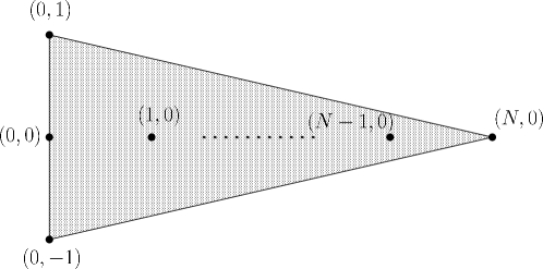
Figure 12: The Newton polygon for $SU(N)$ theory.

By understanding the above polygon as the Newton polygon, we employ the following Laurent polynomial.

$$f_{SU(N)}(x,y)=Q_{N}(x)-(R\Lambda)^{N}\bigl{(}y+y^{-1}\bigr{)}\,,$$ (2.35)

where $Q_{N}(x)$ denotes a monic polynomial of degree $N$ with real coefficients. Let $\beta_{1},\ldots,\beta_{N}$ be roots of $Q_{N}(x)$.

$$Q_{N}(x) = x^{N}+b_{1}x^{N-1}+\cdots+b_{N}$$ (2.36)

$$= \prod_{r=1}^{N}(x-\beta_{r})\,.$$ (2.37)

All the roots are assumed to be real positive numbers. They are arranged in numerical order $0<\beta_{1}<\cdots<\beta_{N}$. We also make $\Lambda$ very small so that $Q_{N}(x)\pm 2(R\Lambda)^{N}$ have $N$ distinct real positive roots.

Figure 13: The zero locus $V_{f_{SU(N)}}$.

We observe the amoeba of $f_{SU(N)}$. The zero locus $V_{f_{SU(N)}}$ in $(\mathbb{C}^{*})^{2}$ is a four-punctured surface. It is a hyperelliptic curve of genus $N-1$ (Figure 13). The amoeba $\mathcal{A}_{f_{SU(N)}}$ is the image $\mathrm{Log}\bigl{(}V_{f_{SU(N)}}\bigr{)}$. The hyperelliptic involution $y\leftrightarrow y^{-1}$ induces the involution $v\leftrightarrow-v$ on the amoeba. Shape of the amoeba depends sharply on the parameters $\Lambda$ and $\beta_{r}$. When the parameters are set as above, the amoeba spreads its four tentacles and these asymptotes are

$$v=\pm Nu\,,\hskip 28.45274ptv=\pm\delta_{N}\,,$$ (2.38)

where $\delta_{N}$ is a positive constant given by

$$\delta_{N}=\frac{1}{R}\ln\left\{\frac{|b_{N}|}{2(R\Lambda)^{N}}+\sqrt{\Bigl{(}\frac{|b_{N}|}{2(R\Lambda)^{N}}\Bigr{)}^{2}-1}\right\}\,.$$ (2.39)

The amoeba complement ${}^{c}\mathcal{A}_{f_{SU(N)}}$ has $N+3$ connected components that correspond exactly to integer lattice points of the Newton polygon $\Delta_{f_{SU(N)}}$. Four of them are unbounded components lying between the tentacles. All the other components are bounded components enclosed by the amoeba. That is to say, there are $N-1$ holes in the amoeba. An example of the amoeba is drawn in Figure 14.

Figure 14: The amoeba of $f_{SU(2)}$.

Consider the section of the amoeba along the $u$-axis. Let us write

$$Q_{N}(x)-2(R\Lambda)^{N}\cos\theta_{y}=\prod_{r=1}^{N}\bigl{(}x-\beta_{r}(\theta_{y})\bigr{)}\,.$$ (2.40)

All the $\beta_{r}(\theta_{y})$’s become real positive numbers since $\Lambda$ is made so small. They are distinct and are arranged in numerical order $0<\beta_{1}(\theta_{y})<\cdots<\beta_{N}(\theta_{y})$. Bands of the amoeba, which are the longitudinal section of the amoeba along the $u$-axis, consist of $N$ segments with finite length.

$$\mbox{Bands : }\bigsqcup_{r=1}^{N}I_{r}\,,~{}~{}~{}~{}I_{r}=\left\{\frac{1}{R}\log\beta_{r}(\theta_{y})\in\mathbb{R}\ :\ 0\leq\theta_{y}<2\pi\right\}\,.$$ (2.41)

Similarly to the $U(1)$ case, we call the complement of the bands the gap. Two ends of the $r$-th band $I_{r}$ are $\frac{1}{R}\log\beta_{r}^{+}$ and $\frac{1}{R}\log\beta_{r}^{-}$, where we put $\beta^{+}_{r}=\beta_{r}(0)$ and $\beta_{r}^{-}=\beta_{r}(\pi)$. The $r$-th band is a segment between $\frac{1}{R}\log\beta_{r}^{-}$ and $\frac{1}{R}\log\beta_{r}^{+}$ on the $u$-axis. Whether $\beta_{r}^{-}<\beta_{r}^{+}$ or $\beta_{r}^{+}<\beta_{r}^{-}$ depends on $N$ and $r$.

$$\begin{array}[]{ll}\beta_{r}^{-}<\beta_{r}^{+}&~{}~{}~{}\mbox{if $Nr=$even}\,,\\[5.69054pt] \beta_{r}^{+}<\beta_{r}^{-}&~{}~{}~{}\mbox{if $Nr=$odd}\,.\end{array}$$ (2.44)

The Ronkin function $N_{f_{SU(N)}}$ is given by

$$N_{f_{SU(N)}}(u,v)=\frac{1}{R}\,\frac{1}{(2\pi i)^{2}}\int_{\scriptstyle|x|=e^{Ru}\atop\scriptstyle|y|=e^{Rv}}\frac{dx}{x}\frac{dy}{y}\,\log\left|f_{SU(N)}(x,y)\right|\,.$$ (2.45)

We will concentrate our attention on the Ronkin function over the $u$-axis. The gradient along the $u$-axis can be written as

$$\frac{\partial N_{f_{SU(N)}}}{\partial u}\bigg{|}_{v=0}=\sum_{r=1}^{N}\frac{1}{(2\pi i)^{2}}\int_{|y|=1}\frac{dy}{y}\int_{|x|=e^{Ru}}\frac{dx}{x-\beta_{r}(\theta_{y})}\,.$$ (2.46)

There are $N$ poles in the above integrand. Each band holds exactly one pole and every pole depends on $\theta_{y}$. It is obvious that every summand in (2.46) takes the same form as in the previous $U(1)$ case.

Consider the $r$-th summand in (2.46). The residue integral vanishes unless $u$ satisfies the inequality $e^{Ru}\geq\beta_{r}(\theta_{y})$. When $u$ is off the $r$-th band $I_{r}$, this condition is irrespective of $\theta_{y}$. We have

$$\frac{1}{(2\pi i)^{2}}\int_{|y|=1}\frac{dy}{y}\int_{|x|=e^{Ru}}\frac{dx}{x-\beta_{r}(\theta_{y})}=\left\{\begin{array}[]{ll}0&\hskip 8.53581pt\mbox{if}~{}~{}u<\min\bigl{(}\,\frac{1}{R}\log\beta_{r}^{+},\frac{1}{R}\log\beta_{r}^{-}\,\bigr{)}\,,\\[8.53581pt] 1&\hskip 8.53581pt\mbox{if}~{}~{}u>\max\bigl{(}\,\frac{1}{R}\log\beta_{r}^{+},\frac{1}{R}\log\beta_{r}^{-}\,\bigr{)}\,.\end{array}\right.$$ (2.49)

On the other hand, when $u$ is on the $r$-th band $I_{r}$, we have to read the inequality $e^{Ru}\geq\beta_{r}(\theta_{y})$ as a condition on $\theta_{y}$. It should be noted that this reading depends on whether $\beta_{r}^{-}<\beta_{r}^{+}$ or $\beta_{r}^{+}<\beta_{r}^{-}$. We first consider the case of $\beta_{r}^{-}<\beta_{r}^{+}$. The function $Q_{N}(x)$ increases over $[\beta_{r}^{-},\beta_{r}^{+}]$. Thus the inequality can be translated to $Q_{N}(e^{Ru})\geq Q_{N}(\beta_{r}(\theta_{y}))=2(R\Lambda)^{N}\cos\theta_{y}$ over the band $I_{r}$. So we obtain the following condition for $\theta_{y}$.

$$\cos\theta_{y}\leq\frac{Q_{N}(e^{Ru})}{2(R\Lambda)^{N}}\,.$$ (2.50)

Therefore the $r$-th summand of this case becomes

$$\frac{1}{(2\pi i)^{2}}\int_{|y|=1}\frac{dy}{y}\int_{|x|=e^{Ru}}\frac{dx}{x-\beta_{r}(\theta_{y})} = \frac{1}{2\pi}\int_{\cos\theta_{y}\leq\frac{Q_{N}(e^{Ru})}{2(R\Lambda)^{N}}}d\theta_{y}\cdot 1$$ (2.51)

$$= N-r+1+\frac{1}{\pi}\arccos\left\{\frac{Q_{N}(e^{Ru})}{2(R\Lambda)^{N}}\right\}\,,$$

where the branch of the arccosine is fixed by choosing $\arccos(0)=\left(r-N-\frac{1}{2}\right)\pi$. We turn to consider the case of $\beta_{r}^{+}<\beta_{r}^{-}$. In this case, $Q_{N}(x)$ decreases over $[\beta_{r}^{+},\beta_{r}^{-}]$. So the inequality means $Q_{N}(e^{Ru})\leq Q_{N}(\beta_{r}(\theta_{y}))=2(R\Lambda)^{N}\cos\theta_{y}$ over the band $I_{r}$. The condition for $\theta_{y}$ becomes

$$\cos\theta_{y}\geq\frac{Q_{N}(e^{Ru})}{2(R\Lambda)^{N}}\,.$$ (2.52)

The $r$-th summand of this case leads to the same expression as (2.51).

By summing up the above ingredients, we obtain the following expression for the gradient of the Ronkin function along the $u$-axis.

$$\frac{\partial N_{f_{SU(N)}}}{\partial u}\bigg{|}_{v=0}=\left\{\begin{array}[]{ll}r&\begin{array}[]{l}\mbox{if}~{}~{}\max\bigl{(}\frac{1}{R}\log\beta_{r}^{\pm}\bigr{)}<u<\min\bigl{(}\frac{1}{R}\log\beta_{r+1}^{\pm}\bigr{)}\\[-1.42262pt] \hskip 14.22636pt(r=0,1,\cdots,N)\,,\end{array}\\[19.91692pt] N+\frac{1}{\pi}\arccos\left\{\frac{Q_{N}(e^{Ru})}{2(R\Lambda)^{N}}\right\}&\begin{array}[]{l}\mbox{if}~{}~{}u\in I_{s}\\[-1.42262pt] \hskip 14.22636pt(s=1,2,\cdots,N)\,.\end{array}\end{array}\right.$$ (2.59)

We put $\beta_{0}^{\pm}=-\infty$ and $\beta_{N+1}^{\pm}=\infty$ in the above. The graph of $\partial_{u}N_{f_{SU(N)}}\big{|}_{v=0}$ is depicted in Figure 15.

Figure 15: The gradient of the Ronkin function of $f_{SU(3)}$.

Integrating (2.59), we acquire the Ronkin function over the $u$-axis. The Ronkin function is constant over the connected component $E_{(0,0)}$ of the amoeba complement and its height there is $c_{(0,0)}=\delta_{N}+\frac{1}{R}\log(R\Lambda)^{N}$. This gives the boundary condition for the integration. See Figure 16.

We also arrange the expression (2.59) in terms of complex geometry. The zero locus $V_{f_{SU(N)}}$ in $(\mathbb{C}^{*})^{2}$ is written as

$$y+y^{-1}=\frac{Q_{N}(e^{Rz})}{(R\Lambda)^{N}}\,,$$ (2.60)

where $z$ denotes the cylindrical coordinate of $\mathbb{C}^{*}$. This hyperelliptic curve is a double cover of the $\mathbb{C}^{*}$ with $2N$ branch points (Figure 13). The branch points locate at the ends of the bands (2.41). The holomorphic function $y$ has $N$ cuts along the bands on the Riemann sheet and takes values at the unit circle over the bands. In particular, it is $\pm 1$ at the branch points. Using $y$, we can rewrite (2.59) as follows.

$$\frac{\partial N_{f_{SU(N)}}}{\partial u}\bigg{|}_{v=0}=\Re\Bigl{(}N+\frac{1}{\pi i}\log y(u-i0)\Bigr{)},$$ (2.61)

where we choose $\arg y(u-i0)$ so that it increases along the $u$-axis from $-N\pi$ to $0$.

Note added :  It was shown in [38] (see also [32]) that expression of the gradient like (2.61) holds commonly for the Ronkin functions of Harnack curves, where a curve is Harnack if and only if the map from the curve to its amoeba is two-to-one over the amoeba interior. This was pointed out by A. Okounkov after the original version of this paper was submitted to e-print archives. The authors are grateful to him.

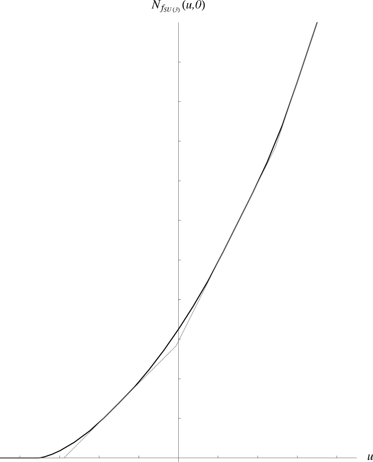
Figure 16: The Ronkin function of $f_{SU(3)}$ over the $u$-axis.

3 Ronkin’s functions and $5d$ SUSY gauge theories

By identifying the parameters of the Laurent polynomials with the gauge theory order parameters in suitable manners, their Ronkin functions relate with instanton countings of five-dimensional supersymmetric gauge theories. The so-called Nekrasov formulae for the exact gauge theory prepotentials have a description in terms of random plane partitions. The Ronkin functions over the $u$-axis turn to be identified with integrations of scaled densities of the main diagonal partitions in the statistical models at the thermodynamic limit. Thus the Ronkin functions are the counting functions.

3.1 A model of random plane partitions

A partition $\lambda=(\lambda_{1},\lambda_{2},\cdots)$ is a sequence of non-negative integers satisfying $\lambda_{i}\geq\lambda_{i+1}$ for all $i\geq 1$. Partitions are often identified with the Young diagrams as seen in Figure 17.

Figure 17: The Young diagram and the Maya diagram

The size is defined by $|\lambda|=\sum_{i\geq 1}\lambda_{i}$, which is the total number of boxes of the diagram. A plane partition $\pi$ is an array of non-negative integers satisfying $\pi_{ij}\geq\pi_{i+1j}$ and $\pi_{ij}\geq\pi_{ij+1}$ for all $i,j\geq 1$. Plane partitions are identified with the three-dimensional Young diagrams. The three-dimensional diagram $\pi$ is a set of unit cubes such that $\pi_{ij}$ cubes are stacked vertically on each $(i,j)$-element of $\pi$. See Figure 18.

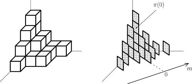
Figure 18: The $3d$ Young diagram and the diagonal slices.

The size is defined by $|\pi|=\sum_{i,j\geq 1}\pi_{ij}$, which is the total number of cubes of the diagram. Diagonal slices of $\pi$ become partitions. Let $\pi(m)$ denote the partition along the $m$-th diagonal slice. In particular, $\pi(0)$ is the main diagonal partition. This series of partitions satisfies the condition

$$\cdots\prec\pi(-2)\prec\pi(-1)\prec\pi(0)\succ\pi(1)\succ\pi(2)\succ\cdots,$$ (3.1)

where $\mu\succ\nu$ means the interlace relation between two partitions $\mu$ and $\nu$.

$$\mu\succ\nu~{}~{}~{}\Longleftrightarrow~{}~{}~{}\mu_{1}\geq\nu_{1}\geq\mu_{2}\geq\nu_{2}\geq\mu_{3}\geq\cdots.$$ (3.2)

We first consider a statistical model of plane partitions defined by the following partition function.

$$Z(q,Q) \equiv \sum_{\pi}\,q^{|\pi|}\,Q^{|\pi(0)|}\,,$$ (3.3)

where $q$ and $Q$ are indeterminate. The Boltzmann weight consists of two parts. The first contribution comes from the energy of plane partitions, and the second contribution is a chemical potential for the main diagonal partitions. The condition (3.1) suggests that plane partitions are certain evolutions of partitions by the discretized time $m$. This leads to a hamiltonian formulation for the model. In particular, the transfer matrix approach developed in [22] express the partition function (3.3) in terms of two-dimensional conformal field theory.

We can interpret the random plane partitions as a $q$-deformation of random partitions. It may be seen by rewriting (3.3) as

$$Z(q,Q)=\sum_{\lambda}\,Q^{|\lambda|}\,\Bigl{(}\sum_{\pi(0)=\lambda}\,q^{|\pi|}\Bigr{)}\,.$$ (3.4)

Partitions $\lambda$ in the above are thought of as the ensemble of the model after summing over plane partitions that main diagonal partitions are $\lambda$. By using the transfer matrix approach [22], the above factorization yields

$$Z(q,Q)=\sum_{\lambda}Q^{|\lambda|}s_{\lambda}(q^{\frac{1}{2}},q^{\frac{3}{2}},\cdots)^{2},$$ (3.5)

where $s_{\mu}(q^{\frac{1}{2}},q^{\frac{3}{2}},\cdots)$ is the Schur function $s_{\mu}(x_{1},x_{2},\cdots)$ of infinitely many variables specialized at $x_{i}=q^{i-\frac{1}{2}}$ [19].

The statistical model gives rise to a description of five-dimensional ${\cal N}=1$ supersymmetric Yang-Mills theories [20]. To contact with the $SU(N)$ gauge theory, we need to identify the indeterminates $q$ and $Q$ with the following field theory variables.

$$q=e^{-\frac{R}{N}\hbar},~{}~{}~{}Q=(R\Lambda)^{2},$$ (3.6)

where $R$ is the radius of $S^{1}$ in the fifth dimension, and $\Lambda$ is the lambda parameter of the underlying four-dimensional field theory.

3.2 Thermodynamic limit and variational problem

The thermodynamic limit is achieved by letting $\hbar\rightarrow 0$. By summing up partitions $\lambda$ in (3.5), we obtain

$$Z(q,Q)=\prod_{n=1}^{+\infty}(1-Qq^{n})^{-n}.$$ (3.7)

The average numbers of cubes and boxes of plane partitions and the main diagonal partitions can be computed from (3.7). By using the identification (3.6), the mean values near the thermodynamic limit become respectively of orders $\hbar^{-3}$ and $\hbar^{-2}$. In particular, we have

$$\lim_{\hbar\rightarrow 0}\Bigl{(}\frac{\hbar}{N}\Bigr{)}^{3}\langle|\pi|\rangle=\frac{2}{R^{3}}Li_{3}(Q)\,,\hskip 28.45274pt\lim_{\hbar\rightarrow 0}\Bigl{(}\frac{\hbar}{N}\Bigr{)}^{2}\langle|\pi(0)|\rangle=\frac{1}{R^{2}}Li_{2}(Q)\,.$$ (3.8)

This implies that, as $\hbar$ goes to zero, a plane partition $\pi$ that dominates is a plane partition of order $\hbar^{-3}$. Similarly, its main diagonal partition $\pi(0)$ or $\lambda$ becomes a partition of order $\hbar^{-2}$. To realize the thermodynamic limit, it becomes necessary to rescale plane partitions and partitions relevantly.

3.2.1 Scaling partitions

We provide a description of the scaling of partitions at the thermodynamic limit. Use of the Maya diagram becomes helpful. For a partition $\lambda$, the Maya diagram $K(\lambda)\subset\mathbb{Z}$ is a set of the integers $x_{i}(\lambda)\equiv-\lambda_{i}+i$, where $i\in\mathbb{Z}_{\geq 1}$. An example of the Maya diagram can be found in Figure 17. For the later convenience, we associate partitions with charges. We denote such a charged partition by $(\lambda,p)$, where $p\in\mathbb{Z}$ is the charge. The Maya diagram $K(\lambda,p)$ is a set of the integers $x_{i}(\lambda)+p$, that is the parallel transport of $K(\lambda)$ by $p$ along the $x$-axis.

For a charged partition $(\lambda,p)$ or the Maya diagram $K(\lambda,p)$, we introduce the density as

$$\rho_{bare}(x|\lambda;p)\equiv\sum_{i=1}^{+\infty}\delta(x-x_{i}(\lambda)-p)\,.$$ (3.9)

The above is not sensitive to the charge since $p$ can be absorbed into the shift of $x$. We can modify (3.9) as

$$\rho_{reg}(x|\lambda;p)=\sum_{i=1}^{+\infty}\delta(x-x_{i}(\lambda)-p)-\sum_{i=1}^{+\infty}\delta(x-i)\,,$$ (3.10)

where the subtraction is prescribed so that it satisfies the normal-ordering condition.

$$\int_{-\infty}^{+\infty}dx\rho_{reg}(x|\lambda;p)=-p\,.$$ (3.11)

Let $\lambda$ be a partition of order $\hbar^{-2}$ and $p$ be of order $\hbar^{-1}$. We may think of $x_{i}(\lambda)$ as quantities of order $\hbar^{-1}$. We regard that elements of such a partition could be suffixed by $s\in\mathbb{R}_{\geq 0}$ rather than $i\in\mathbb{Z}_{\geq 1}$, and that these two kinds of indices relate with each other by $i=s/\hbar$ when $\hbar$ is nearly zero. As $\hbar\rightarrow 0$, $x_{i}(\lambda)$ are rescaled to a certain function $u(s|\lambda)$, which takes value in $\mathbb{R}$.

$$x_{i}(\lambda)=\frac{N}{\hbar}u(s|\lambda)+O(\hbar^{0})\,.$$ (3.12)

As for the charge we rescale $p$ to $a\in\mathbb{R}$ by

$$p=\frac{N}{\hbar}a\,.$$ (3.13)

It should be noticed that $x_{1}(\lambda),x_{2}(\lambda),\cdots$ is a strictly increasing series which satisfies the conditions that $x_{i}(\lambda)\leq i$ for $\forall i$ and that $x_{i}(\lambda)=i$ for $i\geq l(\lambda)$, where $l(\lambda)$ is the length of $\lambda$. The function $u(s|\lambda)$ becomes a strictly increasing function, and satisfies the conditions that $u(s|\lambda)\leq s/N$ for $\forall s$ and that $u(s|\lambda)=s/N$ for $s\geq\zeta$, where $\zeta$ is a finite constant obtained from $l(\lambda)$. The inverse of $u(s|\lambda)$ exists and is denoted by $s(u|\lambda)$. It becomes a nondecreasing function over $\mathbb{R}$, and satisfies the conditions that $s(u|\lambda)=Nu$ for $u\geq\xi$ and $s(u|\lambda)=0$ for $u\leq-\xi$, where $\xi$ is a certain positive constant which one may take $\xi=\zeta/N$.

As $\hbar\rightarrow 0$, we also scale the density (3.9) by using (3.12) and (3.13). In particular, taking account of (3.12), we rescale $x$ to $u\in\mathbb{R}$ by $x=Nu/\hbar$. Then the scaling limit is read as

$$\lim_{\hbar\rightarrow 0}\rho_{bare}(x=Nu/\hbar\,|\lambda;\,p=Na/\hbar)=\rho(u-a|\lambda)\,,$$ (3.14)

where

$$\rho(u|\lambda)\equiv\frac{1}{N}\frac{ds(u|\lambda)}{du}\,.$$ (3.15)

The behavior of the function $s(u|\lambda)$ implies that the scaled density $\rho(u|\lambda)$ takes values in $[0,1]$. It also implies that $d\rho(u|\lambda)/du$ has a compact support in $\mathbb{R}$ and satisfies

$$\int_{-\infty}^{+\infty}du\frac{d\rho(u|\lambda)}{du}=1\,.$$ (3.16)

Similarly to (3.14), the regularized density $\rho_{reg}(x|\lambda;p)$ is scaled to $\rho(u-a|\lambda)-\rho(u|\emptyset)$. The scaled density of the empty partition is $\rho(u|\emptyset)=\theta(u)$, where $\theta(u)$ denotes the step function, that is, $\theta(u)=1$ for $u\geq 0$ and $0$ for $u<0$. Applying a partial integration and combining with (3.16), we can translate the condition (3.11) as follows.

$$\int_{-\infty}^{+\infty}duu\frac{d\rho(u|\lambda)}{du}=0\,.$$ (3.17)

The scaled density $\rho(u|\lambda)$ relates with the shape of the Young diagram. A piecewise linear curve that traces the upper side of the Young diagram positioned as in Figure 17 and extends over $\mathbb{R}$ by $|x|$, is called profile of $\lambda$. The scaling limit of the profile becomes the graph of a certain function $P(u|\lambda)$. This function relates with the scaled density by

$$\frac{dP(u|\lambda)}{du}=-1+2\rho(u|\lambda)\,.$$ (3.18)

3.2.2 The variational problem

In the description (3.5), each partition $\lambda$ has the Boltzmann weight $Q^{|\lambda|}s_{\lambda}(q^{\frac{1}{2}},q^{\frac{3}{2}},\cdots)^{2}$, where the parameters are identified with $q=\exp(-R\hbar/N)$ and $Q=(R\Lambda)^{2}$. When partitions are scaled according to (3.12), the asymptotic form of their weight is computed in [39] by using the product formula of the (specialized) Schur function [19], and is expressed as a functional of the scaled density. It can be read

$$\log Q^{|\lambda|}s_{\lambda}(q^{\frac{1}{2}},q^{\frac{3}{2}},\cdots)^{2}=-\frac{1}{\hbar^{2}}\Bigl{\{}E[\rho(\cdot|\lambda)]+O(\hbar)\Bigr{\}}\,,$$ (3.19)

where

$$E[\rho(\cdot|\lambda)] = N^{2}\int_{-\infty<u<\underline{u}<+\infty}dud\underline{u}\,\,\rho(u|\lambda)\bigl{(}1-\rho(\underline{u}|\lambda)\bigr{)}\log\Bigl{\{}\frac{\sinh\frac{R}{2}(\underline{u}-u)}{\frac{R}{2}\Lambda}\Bigr{\}}^{2}$$ (3.20)

$$+N^{2}\int_{-\infty}^{+\infty}du\frac{Ru^{3}}{6}\frac{d\rho(u|\lambda)}{du}\,.$$

Near the thermodynamic limit, partitions of order $\hbar^{-2}$ dominate in the statistical model. Their Boltzmann weights are measured by using the energy functional $E$ as $e^{-E/\hbar^{2}}$. Since the thermodynamic limit is achieved by letting $\hbar\rightarrow 0$, this means that it is realized by a classical configuration that minimizes the energy functional. We are thus led to consider a variational problem of the energy functional and to find the minimizer as the stationary configuration.

The minimizer of the energy functional (3.20) should be found from among certain admissible configurations. The admissible configurations are thought of functions $\rho(u)$ that could be obtained as the scaled densities of partitions. They need to take values in $[0,1]$. Furthermore, taking account of (3.16) and (3.17), we require that $d\rho(u)/du$ has a compact support in $\mathbb{R}$ and satisfies the conditions

$$\int_{-\infty}^{+\infty}du\,\,\frac{d\rho(u)}{du} = 1\,,$$ (3.21)

$$\int_{-\infty}^{+\infty}du\,\,u\,\frac{d\rho(u)}{du} = 0\,.$$ (3.22)

To argue the variational problem, it is convenient to rewrite the energy functional in the following form by partial integrations.

$$E[\rho(\cdot)] = \frac{N^{2}}{2}\int_{u\neq\underline{u}}dud\underline{u}\,\,\frac{d\rho(u)}{du}\frac{d\rho(\underline{u})}{d\underline{u}}\gamma(|\underline{u}-u|;\Lambda;R)$$ (3.23)

$$+N^{2}\int_{-\infty}^{+\infty}du\frac{Ru^{3}}{6}\frac{d\rho(u)}{du}\,,$$

where the function $\gamma(u;\Lambda;R)$ has been introduced by the conditions

$$\frac{\partial^{2}\gamma}{\partial u^{2}}(u;\Lambda;R)\,=\,\log\Bigl{(}\frac{\sinh\frac{R}{2}u}{\frac{R}{2}\Lambda}\Bigr{)}\,,$$ (3.24)

$$\gamma(0;\Lambda;R)\,=\,\frac{\partial\gamma}{\partial u}(0;\Lambda;R)\,=0\,.$$ (3.25)

It is clear from the expression (3.23) that variations $\rho\rightarrow\rho+\delta\rho$ of the energy functional lead to the stationary equation

$$\mbox{PP}\int_{-\infty}^{+\infty}d\underline{u}\,\,\frac{\partial\gamma}{\partial u}(|u-\underline{u}|;\Lambda;R)\frac{d\rho(\underline{u})}{d\underline{u}}=-\frac{Ru^{2}}{2}\hskip 19.91692pt\mbox{on}\hskip 8.53581pt\mbox{supp}\,\bigl{(}\frac{d\rho}{du}\bigr{)}\,.$$ (3.26)

The integration symbol in the above means principle part. By differentiating Eq.(3.26) twice with respect to $u$, we get

$$\mbox{PP}\int_{-\infty}^{+\infty}d\underline{u}\,\,\coth\frac{R}{2}(u-\underline{u})\frac{d\rho(\underline{u})}{d\underline{u}}=-1\hskip 19.91692pt\mbox{on}\hskip 8.53581pt\mbox{supp}\,\bigl{(}\frac{d\rho}{du}\bigr{)}\,.$$ (3.27)

The variational problem is now stated to find out a solution $\rho_{\star}(u)$ of the integral equation (3.27) from among the admissible configurations.

The standard argument [24] allows us to reformulate this as a problem to find out a certain analytic function $\Phi(z)$. It may be helpful to consider an analytic function that is realized as the integral transform of a continuous function $\chi(u)$ over the real axis.

$$\Phi_{\chi}(z)=\int_{-\infty}^{+\infty}du\,\,\coth\frac{R}{2}(z-u)\,\chi(u)\,.$$ (3.28)

The above function is regarded as an analytic function on $\mathbb{C}^{*}$ since it is periodic with the period $2\pi i/R$. On the real axis, when one approaches from the upper or the lower half plane, it takes

$$\Phi_{\chi}(u\pm i0)=\mbox{PP}\int_{-\infty}^{+\infty}d\underline{u}\,\,\coth\frac{R}{2}(u-\underline{u})\,\chi(\underline{u})\,\,\mp\frac{2\pi i}{R}\chi(u)\,.$$ (3.29)

Observing the above formula by putting $\chi=d\rho/du$, we deduce the variational problem as follows: Let $\Phi(z)$ be an analytic function that is periodic with the period $2\pi i/R$ and behave at the infinities as

$$\Phi(z)\longrightarrow\pm 1\hskip 14.22636pt\mbox{as}\hskip 5.69054pt\Re z\rightarrow\pm\infty\,.$$ (3.30)

We further suppose that $\Phi(z)$ has a cut on a bounded region $I$ along the real axis and satisfies

$$\begin{array}[]{ll}\Re\hskip 2.84526pt\Phi(u)\,=\,-1&\hskip 17.07164pt\mbox{on}\hskip 5.69054ptI\,,\\ \Im\hskip 2.84526pt\Phi(u)\,=\,0&\hskip 17.07164pt\mbox{on}\hskip 5.69054pt\mathbb{R}\setminus I\,,\end{array}$$ (3.33)

and

$$\frac{R}{4\pi i}\oint_{C}dz\,\,z\Phi(z)\,=\,0\,,$$ (3.34)

where $C$ denotes a contour which encircles the above $I$ anticlockwise (Figure 19).

Figure 19: The cut $I$ and the contour $C$ on the Riemann sheet.

Then the solution $\rho_{\star}$ of the variational problem is given by the imaginary part of $\Phi$ along the real axis as follows.

$$\frac{d\rho_{\star}(u)}{du}=\mp\frac{R}{2\pi}\Im\,\Phi(u\pm i0)\,.$$ (3.35)

In particular, we have $\mbox{supp}\,(d\rho_{\star}/du)=I$.

We note that the conditions (3.30), (3.33) and (3.34) are translations of (3.16), (3.27) and (3.17) respectively.

3.3 $U(1)$ gauge theory and the Ronkin function

We consider the case of the $U(1)$ gauge theory. We put $N=1$. The partition function (3.3) can be identified with the partition function for four-dimensional $\mathcal{N}=2$ supersymmetric $U(1)$ gauge theory on noncommutative $\mathbb{R}^{4}$.

To find out a solution of the variational problem posed at the end of the previous subsection, we test an analytic function of the following form.

$$\Phi(z)=\frac{d}{dz}\Bigl{(}-z+\frac{2}{R}\log y\Bigr{)}\,,$$ (3.36)

where

$$y+y^{-1}=\frac{1}{R\Lambda}\bigl{(}e^{Rz}-\beta\bigr{)}\,.$$ (3.37)

Here $\beta$ is a real parameter and is assumed $\beta>2R\Lambda$.

It is easy to see that the above function satisfies the condition (3.30). Along the real axis, it has a single cut on $[\,\frac{1}{R}\log(\beta-2R\Lambda),\,\frac{1}{R}\log(\beta+2R\Lambda)\,]$. We can also see that it satisfies the condition (3.33). We examine the condition (3.34). Let $C$ be the contour that encircles the above cut anticlockwise on the $z$-plane. We will evaluate the contour integral in (3.34) as follows.

$$\frac{R}{4\pi i}\oint_{C}dz\,\,z\Phi(z) = \frac{1}{2\pi i}\oint_{C}zd\log y$$ (3.38)

$$= \frac{1}{2\pi iR}\int_{|y|=1}\frac{dy}{y}\log\left\{R\Lambda(y+y^{-1})+\beta\right\}.$$

The last integration can be computed by applying the classical Jensen formula in complex analysis and gives rise to

$$\frac{R}{4\pi i}\oint_{C}dz\,\,z\Phi(z)=-\frac{1}{R}\log\frac{\beta-\sqrt{\beta^{2}-4(R\Lambda)^{2}}}{2(R\Lambda)^{2}}\,.$$ (3.39)

The vanishing of the contour integration fixes $\beta$ as

$$\beta=1+(R\Lambda)^{2}\,.$$ (3.40)

We thus obtain the solution $\rho^{U(1)}_{\star}(u)$ by letting $\beta=1+(R\Lambda)^{2}$ in (3.37). Let us summarize this as follows.

$$\frac{d\rho_{\star}^{U(1)}}{du}(u)=\mp\frac{1}{\pi}\,\Im\,\frac{d\log y}{dz}(u\pm i0)\,,$$ (3.41)

where

$$y+y^{-1}=\frac{1}{R\Lambda}\bigl{(}e^{Rz}-1-(R\Lambda)^{2}\bigr{)}\,.$$ (3.42)

We note that the above solution is precisely that obtained in [39] by the WKB analysis of the fermion wave function.

We specialize the Laurent polynomial $f_{U(1)}$, which is given in (2.13), by choosing $\beta=1+(R\Lambda)^{2}$. The above solution can be expressed by using the Ronkin function of this $f_{U(1)}$. By comparing (3.41) with (2.34), we find

$$\rho_{\star}^{U(1)}(u)=\frac{\partial N_{f_{U(1)}}(u,0)}{\partial u}\,.$$ (3.43)

This means that the Ronkin function over the $u$-axis is an integration of the scaled density of the main diagonal partitions that realizes the thermodynamic limit.

$$N_{f_{U(1)}}(u,0)=\int_{-\infty}^{u}d\underline{u}\,\,\rho_{\star}^{U(1)}(\underline{u})+\mbox{const.}$$ (3.44)

Let $P_{\star}^{U(1)}(u)$ be the limit shape of the Young diagrams obtained from $\rho_{\star}^{U(1)}(u)$ by using the relation (3.18). We can write (3.44) as follows.

$$N_{f_{U(1)}}(u,0)=\frac{1}{2}\Bigl{(}P_{\star}^{U(1)}(u)+u\Bigr{)}+\mbox{const.}$$ (3.45)

3.4 Random plane partitions and $SU(N)$ gauge theory

There is a bijective correspondence between charged partitions $(\mu,p)$ and $N$ charged partitions $\{(\lambda^{(r)},p_{r})\}^{N}_{r=1}$. This arises from a division algorithm for the Young diagrams analogous to that for integers. The correspondence is neatly described by using the Maya diagrams as follows.

$$K(\mu,p)=\bigcup_{r=1}^{N}\,\,\iota_{r}\bigl{(}K(\lambda^{(r)},p_{r})\bigr{)}\,,$$ (3.46)

where $\iota_{r}$ $\mathbb{Z}\hookrightarrow\mathbb{Z}$ denotes an injective map given by $\iota_{r}(m)=Nm+r-N$, and we have $\iota_{r}\bigl{(}K(\lambda^{(r)},p_{r})\bigr{)}=N\,K(\lambda^{(r)},p_{r})+r-N$. It can be seen that the charges are conserved in (3.46).

$$p=\sum_{r=1}^{N}p_{r}\,.$$ (3.47)

In terms of the Young diagrams the correspondence (3.46) is seen as Figure 20.

Figure 20: Partition corresponding to three charged partitions $(\lambda_{1},p_{1})=((2,1),-7)$, $(\lambda_{2},p_{2})=((3,2),-1)$ and $(\lambda_{3},p_{3})=((3,2),8)$ by (3.46). Three clusters of bold boxes correspond respectively to the three partitions.

By using the above correspondence, the factorization (3.4) or (3.5) is also expressed in terms of $N$ charged partitions $\{(\lambda^{(r)},p_{r})\}^{N}_{r=1}$. Since the factorization was done by using neutral partitions, the charge conservation says that the charges $p_{r}$ satisfy the $SU(N)$ condition

$$\sum_{r=1}^{N}p_{r}=0\,.$$ (3.48)

After including the summation over partitions $\lambda^{(r)}$ implicitly in each component of the factorization, let us factor the partition function into

$$Z(q,Q)=\sum_{\{p_{r}\}}Z_{SU(N)}(\{p_{r}\};q,Q)\,.$$ (3.49)

The above factorization becomes a bridge between the random plane partitions and five-dimensional $\mathcal{N}=1$ supersymmetric $SU(N)$ Yang-Mills. Let $a_{r}$ be the vacuum expectation values of the adjoint scalar in the vector multiplet. We identify the parameters $q,Q$ and $p_{r}$ with the gauge theory parameters as follows.

$$q=e^{-\frac{R}{N}\hbar},\hskip 11.38109ptQ=(R\Lambda)^{2},\hskip 11.38109ptp_{r}=a_{r}/\hbar\,.$$ (3.50)

It is shown [20] that the above identification leads to

$$Z_{SU(N)}(\{p_{r}\};q,Q)=Z_{5d\,\mbox{\scriptsize{SYM}}}(\{a_{r}\};\Lambda,R,\hbar)\,,$$ (3.51)

where the RHS is the exact partition function [8] for five-dimensional $\mathcal{N}=1$ supersymmetric $SU(N)$ Yang-Mills plus the Chern-Simons term having the coupling constant equal to $N$. The five-dimensional theory is living on $\mathbb{R}^{4}\times S^{1}$, where the radius of $S^{1}$ in the fifth dimension is $R$. The scale parameter of the underlying four-dimensional theory is $\Lambda$. In the cases that the Chern-Simons coupling constant takes other values, the partition functions can be also retrieved from the statistical model by adding another potential term for the main diagonal partitions in (3.3) [34].

The realization of partitions in terms of multiple charged partitions also plays important roles in multi-instanton calculus on ALE spaces [40],[41]. Combinatorial aspect that becomes key to the calculus is further elucidated in [42].

3.4.1 Scaling multiple charged partitions

Let us consider $N$ charged partitions $\{(\lambda^{(r)},p_{r})\}^{N}_{r=1}$, where each partition $\lambda^{(r)}$ is of order $\hbar^{-2}$ and each charge $p_{r}$ is of order $\hbar^{-1}$. Each charged partition is treated by the following scalings.

$$x_{i_{r}}(\lambda^{(r)}) = u(s_{r}|\lambda^{(r)})/\hbar+O(\hbar^{0})\,,$$ (3.52)

$$p_{r} = a_{r}/\hbar\,,$$ (3.53)

where $s_{r}\in\mathbb{R}_{\geq 0}$ has been introduced by $i_{r}=s_{r}/\hbar$.

Together with the above scalings, the correspondence leads to a scaling of the charged partition $(\mu,p)$ in the forms (3.12) and (3.13). The density of $(\mu,p)$ is expressed in terms of those of $(\lambda^{(r)},p_{r})$ as follows.

$$\rho_{bare}(x|\mu;p)=\frac{1}{N}\sum_{r=1}^{N}\rho_{bare}\bigl{(}\frac{x-r+N}{N}|\lambda^{(r)};p_{r}\bigr{)}\,.$$ (3.54)

We will obtain the scaling limit of this relation. We rescale $x$ to $u$ by $x=Nu/\hbar$. For each charged partition, the inverse of $u(s_{r}|\lambda^{(r)})$ exists, as follows from (3.52), and is denoted by $s_{r}(u|\lambda^{(r)})$. It is a nondecreasing function over $\mathbb{R}$, and satisfies the conditions that $s_{r}(u|\lambda)=u$ for $u\geq\xi_{r}$ and $s_{r}(u|\lambda^{(r)})=0$ for $u\leq-\xi_{r}$, where $\xi_{r}$ is a certain positive constant. By using (3.52) and (3.53), the scaling limit of each density becomes

$$\lim_{\hbar\rightarrow 0}\rho_{bare}(x=u/\hbar\,|\lambda^{(r)};\,p_{r}=a_{r}/\hbar)=\rho_{r}(u-a_{r}|\lambda^{(r)})\,,$$ (3.55)

where

$$\rho_{r}(u|\lambda^{(r)})\equiv\frac{ds_{r}(u|\lambda^{(r)})}{du}\,.$$ (3.56)

As for the charged partition $(\mu,p)$, by taking account of (3.14) and (3.15), the scaling limit of the density is $\rho(u-a|\mu)$. Therefore the relation (3.54) leads to

$$\rho(u-a|\mu)=\frac{1}{N}\sum_{r=1}^{N}\rho_{r}(u-a_{r}|\lambda^{(r)})\,,$$ (3.57)

where $Na=\sum_{r=1}^{N}a_{r}$.

Each scaled density $\rho_{r}(u|\lambda^{(r)})$ takes values in $[0,1]$. We also see that $d\rho_{r}(u|\lambda^{(r)})/du$ has a compact support in $\mathbb{R}$ and satisfies

$$\int_{-\infty}^{+\infty}du\,\frac{d\rho_{r}(u|\lambda^{(r)})}{du} = 1\,,$$ (3.58)

$$\int_{-\infty}^{+\infty}du\,u\frac{d\rho_{r}(u|\lambda^{(r)})}{du} = 0\,.$$ (3.59)

At this stage it is convenient to impose the $SU(N)$ condition (3.48) on the charges. This means that $a_{r}$ are taken so that $\sum_{r=1}^{N}a_{r}=0$. It follows from (3.57) that $d\rho(u|\mu)/du$ is supported on $\cup_{r=1}^{N}I_{r}$, where $I_{r}$ denotes the support of $d\rho_{r}(u-a_{r}|\lambda^{(r)})/du$ and is thought to be a certain segment centered around $a_{r}$. These bands become disjointed when $a_{r}$ are sufficiently separated from one another. In such a circumstance, by using (3.57), it is possible to rewrite (3.58) and (3.59) as follows.

$$\int_{I_{r}}du\,\frac{d\rho(u|\mu)}{du} = 1/N\,,$$ (3.60)

$$\int_{I_{r}}du\,u\frac{d\rho(u|\mu)}{du} = a_{r}/N\,.$$ (3.61)

Figure 21: A typical behavior of the density at small $\hbar$.

3.4.2 The variational problem

We would like to consider the thermodynamic limit of each component that appears in the factorization (3.49). In what follows, we impose the $SU(N)$ condition on the charges. We also fix $a_{r}$ so that they are sufficiently separated from one another. Without any loss it is enough to consider the case of $a_{1}<a_{2}<\,\cdots\,<a_{N}$. By taking account of the previous study of the $U(1)$ gauge theory, the thermodynamic limit we are investigating now is realized by a configuration that minimizes the energy functional with keeping $a_{r}$ fixed. Therefore, the relevant variational problem of the energy functional should be restricted within configurations of the scaled densities that are expressible in terms of $N$ charged partitions with the fixed charges. Such configurations may be obtained by restricting the admissible configurations relevantly. By observing (3.60) and (3.61), we require that $d\rho(u)/du$ is supported on $\cup_{r=1}^{N}I_{r}$, where $I_{r}$ are certain disjointed segments, and satisfies there

$$\int_{I_{r}}du\,\frac{d\rho(u)}{du} = 1/N\,,$$ (3.62)

$$\int_{I_{r}}du\,u\frac{d\rho(u)}{du} = a_{r}/N\,.$$ (3.63)

The variational problem is formulated to find out a solution $\rho_{\star}^{SU(N)}$ of the integral equation (3.27) from among the admissible configurations of the above type.

We can also reformulate this as a problem to find out a certain analytic function: Let $\Phi(z)$ be an analytic function that is periodic with the period $2\pi i/R$, and behave at the infinities as $\Phi(z)\longrightarrow\pm 1$ as $\Re\,z\rightarrow\pm\infty$. We suppose that $\Phi(z)$ has a cut on each disjointed segments $I_{r}$ ($r=1,\,\cdots,\,N$) along the real axis and satisfies

$$\begin{array}[]{ll}\Re\hskip 2.84526pt\Phi(u)\,=\,-1&\hskip 17.07164pt\mbox{on}\hskip 5.69054pt\cup_{r=1}^{N}I_{r}\,,\\ \Im\hskip 2.84526pt\Phi(u)\,=\,0&\hskip 17.07164pt\mbox{on}\hskip 5.69054pt\mathbb{R}\setminus\cup_{r=1}^{N}I_{r}\,.\end{array}$$ (3.66)

Let $C_{r}$ be a contour which encircles the cut $I_{r}$ anticlockwise (Figure 22).

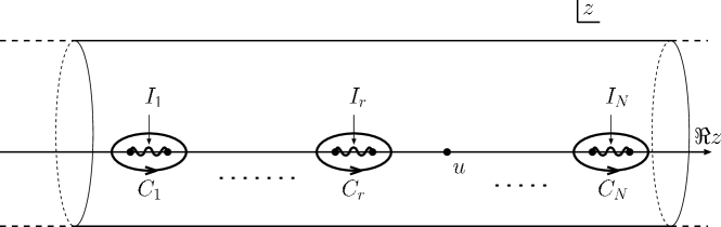
Figure 22: The cuts $I_{r}$ and the contours $C_{r}$ on the Riemann sheet.

We further suppose that $\Phi(z)$ satisfies

$$\frac{R}{4\pi i}\oint_{C_{r}}dz\,\,\Phi(z) = 1/N\,,$$ (3.67)

$$\frac{R}{4\pi i}\oint_{C_{r}}dz\,\,z\Phi(z) = a_{r}/N\,,$$ (3.68)

for each $r$. Then the solution $\rho_{\star}^{SU(N)}$ is given by the imaginary part as follows.

$$\frac{d\rho_{\star}^{SU(N)}(u)}{du}=\mp\frac{R}{2\pi}\Im\,\Phi(u\pm i0)\,.$$ (3.69)

3.5 $SU(N)$ gauge theory and the Ronkin function

We can find the solution $\rho_{\star}^{SU(N)}$ by following the route similar to the $U(1)$ case. Consider the hyperelliptic curve (2.60). This curve is a double cover of $\mathbb{C}^{*}$ with the branch points at two ends of each band $I_{r}$ (2.41). Roots $\beta_{r}$ of the monic polynomial $Q_{N}(x)$ in (2.60) relate with $a_{r}$ by the conditions

$$\frac{1}{2\pi i}\oint_{C_{r}}zd\ln y=a_{r}\,,$$ (3.70)

where $C_{r}$ denotes the contour encircling $I_{r}$ anticlockwise on the Riemann sheet. The analytic function

$$\Phi(z)=\frac{d}{dz}\Bigl{(}-z+\frac{2}{NR}\ln y\Bigr{)}$$ (3.71)

satisfies all the above requirements including (3.66), (3.67) and (3.68). Therefore we obtain

$$\frac{d\rho_{\star}^{SU(N)}(u)}{du}=\mp\frac{1}{N\pi}\,\Im\,\frac{d\ln y}{dz}(u\pm i0)\,.$$ (3.72)

The above solution can be expressed by using the Ronkin function of $f_{SU(N)}$. By comparing (3.72) with (2.61), we find

$$\rho_{\star}^{SU(N)}(u)=\frac{1}{N}\frac{\partial N_{f_{SU(N)}}(u,0)}{\partial u}\,.$$ (3.73)

This means

$$N_{f_{SU(N)}}(u,0)=N\int_{-\infty}^{u}d\underline{u}\,\,\rho_{\star}^{SU(N)}(\underline{u})+\mbox{const.}$$ (3.74)

Let $P_{\star}^{SU(N)}(u)$ be the limit shape of the Young diagrams obtained from $\rho_{\star}^{SU(N)}(u)$ by using the relation (3.18). We can write (3.74) as follows.

$$N_{f_{SU(N)}}(u,0)=\frac{N}{2}\Bigl{(}P_{\star}^{SU(N)}(u)+u\Bigr{)}+\mbox{const.}$$ (3.75)

The variational problem formulated in subsection 3.4.2 could be understood as a variant of that considered in [8], where the variational problem is addressed to the dual partition function for the purpose of proving that the thermodynamic limit realizes the Seiberg-Witten geometry of the prepotential theory. However, that requires the Legendre transformation to reproduce the thermodynamic limit and is likely to become a detour to find a connection with the amoeba and the Ronkin function, while our treatment is straightforward to see the relation.

4 Tropical geometry and crystal

So far, we have seen that the Ronkin function of $f_{SU(N)}$ relates with the limit shape $P^{SU(N)}_{\star}$ as (3.75) under the identification (3.70). We expect that such a relation between the Ronkin functions and the gauge instanton countings is not merely a coincidence but persists further. To support this, we describe a certain degeneration of the amoebas and the Ronkin functions, and provide an interpretation from the viewpoint of statistical models.

The parameter $R$ is identified with the radius of the circle in the fifth dimension of the gauge theories. If one keeps $R\Lambda$ fixed, one can interpret $R$ as the inverse temperature of the statistical models, $R=1/T$, where $T$ denotes the temperature. This means that the large radius limit of the gauge theories corresponds to the low temperature limit of the statistical models. As the temperature approaches to zero, the statistical models get to freeze to the ground states. They are determined by the charges. Crystals are complements of the ground states in the octant and have an interpretation as gravitational quantum foams of the corresponding local Calabi-Yau threefolds [34]. In this section, we argue that the low temperature limits are degenerations of the amoebas known as tropical geometry [35, 36, 37].

The max-plus algebra or tropical semiring $(\mathbb{R},\oplus,\odot)$ is defined by

$$u\oplus v=\max(u,v)\,,\hskip 28.45274ptu\odot v=u+v\,.$$ (4.1)

The tropical semiring is idempotent, as follows from $u\oplus u=u$. If one uses $\oplus$ for addition and $\odot$ for multiplication, a tropical polynomial in two variables is defined as

$$``\,\,\sum_{i,j}a_{ij}u^{i}v^{j}\,\,"=\max_{i,j}\bigl{(}a_{ij}+iu+jv\bigr{)}\,.$$ (4.2)

The quotation mark in the above is used to distinguish the tropical operations from the standard ones. The tropical polynomials are piecewise linear functions and are responsible for some piecewise linear real geometry. Surprisingly, this tropical geometry can be obtained as a certain degeneration of the complex geometry in $(\mathbb{C}^{*})^{2}$.

The idea [37] comes from the so-called Maslov dequantization of real positive numbers. It is a family of semirings $(\mathbb{R},\oplus_{R},\odot_{R})$ parameterized by $R>0$.

$$u\oplus_{R}v=\frac{1}{R}\ln(e^{Ru}+e^{Rv})\,,\hskip 28.45274ptu\odot_{R}v=u+v\,.$$ (4.3)

For each finite $R$, the semiring $(\mathbb{R},\oplus_{R},\odot_{R})$ is isomorphic to the standard semiring of real positive number by the logarithmic map

$$\begin{array}[]{cccc}\mbox{Log}~{}:&(\mathbb{R}_{>0},+,\cdot)&\longrightarrow&(\mathbb{R},\oplus_{R},\odot_{R})\\ &x&\longmapsto&\frac{1}{R}\ln x\,.\end{array}$$ (4.6)

On the other hand, the semiring becomes the tropical semiring at the limit $R\rightarrow\infty$.

$$u\oplus_{\infty}v=u\oplus v\,,\hskip 28.45274ptu\odot_{\infty}v=u\odot v\,.$$ (4.7)

By using the terminology of deformation quantization, this means that the classical semiring of real positive number is a quantized version of the tropical semiring. In other words, the Maslov dequantization says that the tropical semiring is a classical counterpart of the standard semiring of real positive number.

Anticipated from the definition of amoeba, the above dequantization deformation has a counterpart in amoebas. For instance, consider a Laurent polynomial $f(x,y)=\sum_{i,j}b_{ij}x^{i}y^{j}$, where all the $b_{ij}$’s are real positive numbers and supposed to be $b_{ij}=e^{Ra_{ij}}$. As $R\rightarrow\infty$, the corresponding amoeba $\mathcal{A}_{f}$ tends to a piecewise linear curve that is described by the corner set of $``\,\sum_{i,j}a_{i,j}u^{i}v^{j}\,"$ [35, 43].

4.1 Tropical limit of $SU(N)$ amoeba

As in the previous section, we take $a_{r}$ sufficiently separated from each other and arrange them in numerical order $a_{1}<\cdots<a_{N}$. They determine the Laurent polynomial $f_{SU(N)}(x,y)$, given in (2.35), by using the conditions (3.70). We first study degeneration of the corresponding amoeba as $R\rightarrow\infty$. The limit is taken with keeping $a_{1},\cdots,a_{N}$ and $R\Lambda$ fixed. This implies that $\Lambda$ behaves as $O(1/R)$. The thermal fluctuations of the statistical model are suppressed at the low temperature, and each band $I_{r}$ of the density shrinks to the point $a_{r}$. This means that, when $R$ becomes very large, the parameters of the Laurent polynomial (2.35) are $\beta_{r}\approx e^{Ra_{r}}$. We examine how the part of the amoeba within the strip $a_{r}<u<a_{r+1}$ behaves under the above limit. The parts extending to the infinities can be included, by considering the cases of $r=0,\,N$ putting $a_{0}=-\infty$ and $a_{N+1}=+\infty$. It is seen that both $e^{Ra_{s}}x^{-1}$ ($1\leq s\leq r$) and $e^{-Ra_{s}}x$ ($r+1\leq s\leq N$) vanish as $R\rightarrow\infty$, if $x$ satisfies $a_{r}<\frac{1}{R}\ln|x|<a_{r+1}$. By noting this, we can describe effectively the zero locus which is mapped to within the strip as

$$y^{\pm 1}-\frac{(-)^{N-r}}{(R\Lambda)^{N}}e^{R\sum_{s=r+1}^{N}a_{s}}x^{r}=0\,,$$ (4.8)

where $y^{\pm 1}$ are chosen so that $y$ for $|y|>1$, and $y^{-1}$ for $|y|<1$. This shows that the amoeba within the strip $a_{r}<u<a_{r+1}$ degenerates to two linear pieces $v=\pm(ru+\sum_{s=r+1}^{N}a_{s})$ at the limit.

In addition to the above, taking account of the convexity of the connected components of the amoeba complement, the amoeba degenerates to a piecewise linear curve that is described by

$$v=\pm\,\max_{0\leq r\leq N}\Bigl{(}ru+\sum_{s=r+1}^{N}a_{s}\Bigr{)}$$ (4.9)

and

$$\bigcup_{r=1}^{N}\,\Bigl{\{}(a_{r},v)\,\in\mathbb{R}^{2}\,\,;\hskip 8.53581pt|v|\leq ra_{r}+\sum_{s=r+1}^{N}a_{s}\Bigr{\}}\,.$$ (4.10)

An example of the degeneration is depicted in Figure 23.

$\Longrightarrow$

$\Longrightarrow$

Figure 23: Tropical degeneration of the the amoeba of $f_{SU(2)}$.

We turn to consider the behavior of the Ronkin function at the tropical limit. Over the amoeba complement, the Ronkin function is the piecewise linear function $S_{f_{SU(N)}}$. At the tropical limit, where the amoeba degenerates to the above curve, these two functions coincide all over $\mathbb{R}^{2}$. Let us write the piecewise linear function thus obtained as

$$S_{\infty}(u,v)=\lim_{R\rightarrow\infty}\,N_{f_{SU(N)}}(u,v)\,.$$ (4.11)

We can reproduce this $S_{\infty}$ from the piecewise linear curve (4.9) and (4.10), except an addition of a constant to the function. This is because the piecewise linear curve is the corner set of $S_{\infty}$ and the gradient $\nabla S_{\infty}$ equals to the corresponding lattice point of the Newton polygon on each connected component divided by the curve. The constant may be found, for instance, by considering the Ronkin function over $E_{\alpha}$, where $\alpha$ is a vertex of the Newton polygon. In this manner we obtain

$$S_{\infty}(u,v)=\max_{\alpha\in\Delta_{f_{SU(N)}}\cap\,\,\mathbb{Z}^{2}}\Bigl{(}-d_{\alpha}+\langle(u,v),\alpha\rangle\Bigr{)}\,,$$ (4.12)

where

$$\begin{array}[]{lr}d_{(i,0)}=\sum_{r=1}^{i}a_{r}&(1\leq i\leq N)\,,\\ d_{(0,0)}=d_{(0,\pm 1)}=0\,.&\end{array}$$ (4.15)

The set of $(u,v,S_{\infty}(u,v))$ becomes a facet of a three-dimensional polyhedron. We associate a three-dimensional lattice element with each integer lattice point of the Newton polygon by

$$v_{\alpha}=(-\alpha,1)\,\,\,\in\mathbb{Z}^{3}\,,$$ (4.16)

where $\alpha\in\Delta_{f_{SU(N)}}\cap\mathbb{Z}^{2}$. By using these $v_{\alpha}$, we can describe the polyhedron as follows.

$$\mathcal{P}_{SU(N)}=\Bigl{\{}(u,v,w)\in\mathbb{R}^{3}\hskip 2.84526pt;\,\,\langle(u,v,w),v_{\alpha}\rangle+d_{\alpha}\geq 0\hskip 11.38109pt\forall\alpha\in\Delta_{f_{SU(N)}}\cap\mathbb{Z}^{2}\Bigr{\}}\,,$$ (4.17)

where $\langle\,,\,\rangle$ denotes the standard inner product on $\mathbb{R}^{3}$. By comparing the above with (4.12), we see that the facet of this $\mathcal{P}_{SU(N)}$ is actually given by $S_{\infty}$. See Figure 24.

Figure 24: The three-dimensional polyhedron $\mathcal{P}_{SU(N)}$.

4.2 Tropical geometry and quantum foam of local geometry

The polyhedron $\mathcal{P}_{SU(N)}$ has an interpretation in the local geometry and accords with the quantum foam picture [18],[34]. We introduce three-dimensional cones $\sigma_{0},\sigma_{1},\cdots,\sigma_{2N-1}$ by

$$\begin{array}[]{l}\sigma_{2i}=\mathbb{R}_{\geq 0}v_{(i,0)}+\mathbb{R}_{\geq 0}v_{(i+1,0)}+\mathbb{R}_{\geq 0}v_{(0,-1)}\,,\\ \sigma_{2i+1}=\mathbb{R}_{\geq 0}v_{(i,0)}+\mathbb{R}_{\geq 0}v_{(i+1,0)}+\mathbb{R}_{\geq 0}v_{(0,1)}\,.\end{array}$$ (4.20)

All these cones and their faces constitute the fan that describes the local $SU(N)$ geometry $X$. Two-dimensional cones of the fan determine two cycles of the geometry as closed subvarieties that are invariant under the torus action. Cones that are generated by $v_{(k,0)}$ and $v_{(0,-1)}$ determine vanishing cycles in the fibred ALE space, where $1\leq k\leq N-1$. Cone generated by $v_{(1,0)}$ and $v_{(0,0)}$ determines the base $\mathbb{P}^{1}$.

The polyhedron (4.17), more precisely, that rescaled by $1/\hbar$, emerges naturally when quantizations of the local geometry $X$ equipped with a K$\ddot{\mbox{a}}$hler two form $\omega$ on it, are considered. For the consistent quantizations, this $\omega$ needs to be quantized. Topological $A$-model strings suggest the rule that $\omega$ is quantized in the unit of string coupling constant $g_{st}$ [18].

$$\frac{1}{g_{st}}[\omega]\in H^{2}(X,\mathbb{Z})\,.$$ (4.21)

This means that the K$\ddot{\mbox{a}}$hler volumes of two cycles become integral.

$$T_{b}=\frac{1}{g_{st}}\int_{V_{b}}\omega\hskip 5.69054pt\in\mathbb{Z}_{\geq 0}\,,\hskip 22.76219ptT_{k}=\frac{1}{g_{st}}\int_{V_{k}}\omega\hskip 5.69054pt\in\mathbb{Z}_{\geq 0}\hskip 17.07164pt(k=1,\cdots,N-1)\,,$$ (4.22)

where $V_{b}$ and $V_{k}$ denote respectively the base $\mathbb{P}^{1}$ and the vanishing cycles in the fibre that correspond to the cones generated by $v_{(k,0)}$ and $v_{(0,-1)}$. Relation between quantizations of the local geometry and the statistical models is found in [34]. In particular, the integral parameters (4.22) are converted to

$$g_{st}=R\hbar\,,\hskip 22.76219ptT_{b}=-\frac{1}{g_{st}}\log(R\Lambda)^{2N}\,,\hskip 22.76219ptT_{k}=p_{k+1}-p_{k}\,,$$ (4.23)

where $p_{r}$ are integers arranged in numerical order $p_{1}\leq p_{2}\leq\cdots\leq p_{N}$. We will associate these integers with partitions subsequently. We will also impose the $SU(N)$ condition on the integers and slightly restrict allowed values of the parameters so that $\sum_{k=1}^{N-1}kT_{k}\in N\mathbb{Z}_{\geq 0}$.

When the limit $R\rightarrow\infty$ is taken with keeping $R\Lambda$ fixed, it makes $T_{b}$ vanish under the identification (4.23). This implies that we can put $T_{b}=0$ from the beginning, for the present purpose. Let $\omega$ be such a quantized K$\ddot{\mbox{a}}$hler form. The geometric quantization of $(X,\omega)$ requires, first of all, a holomorphic line bundle $L$ on $X$ which the first Chern class equals $c_{1}(L)=[\omega]/g_{st}$. We may take such a line bundle as $L=\mathcal{O}(D)$, where $D$ is a certain toric divisor. Rays or edges of the fan determine closed subvarieties of codimension one that are invariant under the torus action. The divisor is a formal sum of these subvarieties with integral coefficients.

$$D=\sum_{\alpha}p_{\alpha}D_{\alpha}\,,$$ (4.24)

where $D_{\alpha}$ is the subvariety that corresponds to the ray generated by $v_{\alpha}$. The integral parameters (4.22) relate with the above $p_{\alpha}$ by using $c_{1}(\mathcal{O}(D))=[\omega]/g_{st}$. The identification (4.23) allows us to express the coefficients $p_{\alpha}$ by the charges as follows.

$$\begin{array}[]{lc}p_{(i,0)}=\sum_{r=1}^{i}p_{r}&(1\leq i\leq N)\,,\\ p_{(0,0)}=p_{(0,\pm 1)}=0&\,.\end{array}$$ (4.27)

Physical states in the geometric quantization appear as the global sections of $\mathcal{O}(D)$. Thanks to that $X$ is a toric variety, these states are labeled by integer lattice points in a convex polyhedron determined by $D$ [44].

$$\mathcal{P}(X,D)=\Bigl{\{}(u,v,w)\in\mathbb{R}^{3}\hskip 2.84526pt;\,\,\langle(u,v,w),v_{\alpha}\rangle+p_{\alpha}\geq 0\hskip 11.38109pt\forall\alpha\Bigr{\}}\,.$$ (4.28)

Thus space of the physical states has a basis $\chi_{m}$, where $m$ runs over $\mathcal{P}(X,D)\cap\mathbb{Z}^{3}$. Each $\chi_{m}$ is interpreted as a quantum of $(X,\omega)$. The charges $p_{r}$ are scaled to $a_{r}$ by $p_{r}=a_{r}/\hbar$ at the thermodynamic limit or the semiclassical limit. Comparing (4.27) with (4.15), we find $p_{\alpha}=d_{\alpha}/\hbar$. This means that two polyhedra $\mathcal{P}(X,D)$ and $\mathcal{P}_{SU(N)}$ are similar. They relate with each other by the similarity transformation.

$$\mathcal{P}(X,D)=\frac{1}{\hbar}\mathcal{P}_{SU(N)}\,.$$ (4.29)

The number of the physical states is infinite since the cardinality of $\mathcal{P}(X,D)\cap\mathbb{Z}^{3}$ is infinite. In order to manipulate such an infinity, another polyhedron that originates from a local singular geometry is introduced [34].

$$\mathcal{P}_{sing}=\Bigl{\{}(u,v,w)\in\mathbb{R}^{3}\hskip 2.84526pt;\,\,\langle(u,v,w),v_{\alpha}\rangle\geq 0\hskip 11.38109pt\alpha=(0,\pm 1),(N,0),(0,0).\Bigr{\}}\,.$$ (4.30)

The underlying singular geometry is a $\mathbb{Z}_{N}$ orbifold of $\mathcal{O}\oplus\mathcal{O}(-2)\rightarrow\mathbb{P}^{1}$ and is described by the fan consisting of three-dimensional cones $\tau_{1},\tau_{2}$ and their faces.

$$\begin{array}[]{l}\tau_{1}=\mathbb{R}_{\geq 0}v_{(0,0)}+\mathbb{R}_{\geq 0}v_{(N,0)}+\mathbb{R}_{\geq 0}v_{(0,-1)}\,,\\ \tau_{2}=\mathbb{R}_{\geq 0}v_{(0,0)}+\mathbb{R}_{\geq 0}v_{(N,0)}+\mathbb{R}_{\geq 0}v_{(0,1)}\,.\end{array}$$ (4.33)

Figure 25: The three-dimensional polyhedron $\mathcal{P}_{sing}$.

The above polyhedron includes $\mathcal{P}(X,D)$ as an unbounded subset. In [34], the number of the physical states is regularized and is prescribed to be the cardinality of $\mathcal{P}^{c}(X,D)\cap\mathbb{Z}^{3}$, where $\mathcal{P}^{c}(X,D)$ denotes the complement $\mathcal{P}_{sing}\setminus\mathcal{P}(X,D)$. Since it becomes bounded, this relative counting gives a finite answer. When the charges become very large, the cardinality is approximated by the volume measured by the volume element $dudvdw$. Therefore, the number of the physical states becomes $\approx\mbox{Vol}(\mathcal{P}^{c}(X,D))$. The volume can be computed as

$$\mbox{Vol}(\mathcal{P}^{c}(X,D))=\frac{1}{6}\sum_{r>s}^{N}(p_{r}-p_{s})^{3}+\frac{N}{6}\sum_{r=1}^{N}p_{r}^{3}\,,$$ (4.34)

which turns to equal $-D^{3}/3!$, where $D^{3}$ denotes the self-intersection number obtained by intersecting $D$ with itself three times.

The counterpart of the singular geometry is a Laurent polynomial consisting of monomials $1,x^{N},y,y^{-1}$ and reflecting that the geometry is the $\mathbb{Z}_{N}$ orbifold of $\mathcal{O}\oplus\mathcal{O}(-2)\rightarrow\mathbb{P}^{1}$. As such, we will take

$$f^{base}_{SU(N)}(x,y)=x^{N}-1-(R\Lambda)^{2N}-(R\Lambda)^{N}(y+y^{-1})\,.$$ (4.35)

The amoeba of $f^{base}_{SU(N)}$ has four tentacles which asymptote to the straight lines (2.38) but there appears no hole. The tropical limit of the Ronkin function $N_{f^{base}_{SU(N)}}$ becomes

$$S^{base}_{\infty}(u,v)=\max_{\alpha=(0,0),(N.0),(0,\pm 1)}\Bigl{(}\langle(u,v),\alpha\rangle\Bigr{)}\,.$$ (4.36)

This piecewise linear function describes the facet of $\mathcal{P}_{sing}$. The counterpart of $\mathcal{P}^{c}(X,D)$ is the complement $\mathcal{P}^{c}_{SU(N)}=\mathcal{P}_{sing}\setminus\mathcal{P}_{SU(N)}$. This is similar to $\mathcal{P}^{c}(X,D)$.

$$\mathcal{P}^{c}(X,D)=\frac{1}{\hbar}\mathcal{P}^{c}_{SU(N)}\,.$$ (4.37)

Figure 26: The complement $\mathcal{P}^{c}_{SU(N)}=\mathcal{P}_{sing}\setminus\mathcal{P}_{SU(N)}$.

4.3 Tropical geometry and crystal

By using the correspondence (3.46), $N$ charged empty partitions describe a specific partition, which is called $N$ core. Let us consider $N$ charged empty partitions $\{(\emptyset,p_{r})\}_{r=1}^{N}$ that charges are of order $\hbar^{-1}$ and satisfy the $SU(N)$ condition (3.48). The corresponding $N$ core is denoted by $\mu_{N\mbox{\footnotesize{-core}}}$. See Figure 27. Asymptotics of $\mu_{N\mbox{\footnotesize{-core}}}$ at the limit $\hbar\rightarrow 0$ is obtained by scaling each charged empty partition according to (3.52) and (3.53). In particular, the charges are scaled by $p_{r}=a_{r}/\hbar$. The scaled density of $\mu_{N\mbox{\footnotesize{-core}}}$ becomes

$$\rho_{N\mbox{\footnotesize{-core}}}(u)=\rho(u|\mu_{N\mbox{\footnotesize{-core}}})=\frac{1}{N}\sum_{r=1}^{N}\theta(u-a_{r})\,.$$ (4.38)

Each charged empty partition contributes to the above as a step function. Comparing (4.38) with (4.12), one finds that this $\rho_{N\mbox{\footnotesize{-core}}}$ is written by using the piecewise linear function $S_{\infty}$ as

$$\rho_{N\mbox{\footnotesize{-core}}}(u)=\frac{1}{N}\frac{\partial S_{\infty}(u,0)}{\partial u}\,.$$ (4.39)

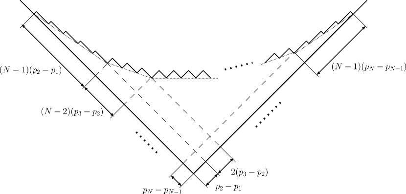
Figure 27: $\mu_{N\mbox{\footnotesize{-core}}}$.

The above expression suggests a certain relation between the $N$ core and the tropical limit of the $SU(N)$ amoeba. To see this, we first compute the energy of $\mu_{N\mbox{\footnotesize{-core}}}$. The charges are arranged $p_{1}\leq\cdots\leq p_{N}$. We evaluate the energy functional (3.23) at $\rho=\rho_{N\mbox{\footnotesize{-core}}}$. The function $\gamma(u;\Lambda;R)$, that is defined by the conditions (3.24) and (3.25), has the expression

$$\gamma(u;\Lambda;R)=\frac{R}{6}u^{3}-\log(R\Lambda)u^{2}-\frac{\pi^{2}}{3R}u+\frac{2}{R^{2}}\left(\zeta(3)-Li_{3}(e^{-Ru})\right)\,.$$ (4.40)

By using this, the energy of $\mu_{N\mbox{\footnotesize{-core}}}$ becomes

$$E[\rho_{N\mbox{\footnotesize{-core}}}] = \frac{R}{6}\left\{\sum_{r>s}^{N}(a_{r}-a_{s})^{3}+N\sum_{r=1}^{N}a_{r}^{3}\right\}-\log(R\Lambda)\sum_{r>s}^{N}(a_{r}-a_{s})^{2}$$ (4.41)

$$-\frac{\pi^{2}}{6R}\sum_{r>s}^{N}(a_{r}-a_{s})+\frac{1}{R^{2}}\sum_{r>s}^{N}\Bigl{(}\zeta(3)-Li_{3}(e^{-R(a_{r}-a_{s})})\Bigr{)}\,.$$

This is the perturbative prepotential of five dimensional $\mathcal{N}=1$ supersymmetric $SU(N)$ Yang-Mills on $\mathbb{R}^{4}\times S^{1}$. The first term of (4.41) dominates when the limit $R\rightarrow\infty$ is taken. Therefore, taking account of (4.34) and (4.37), we obtain the following estimate at the low temperature limit.

$$E[\rho_{N\mbox{\footnotesize{-core}}}]\approx R\cdot\mbox{Vol}\Bigl{(}\mathcal{P}^{c}_{SU(N)}\Bigr{)}\,.$$ (4.42)

A set $\mathcal{M}(p_{1},\cdots,p_{N})$ denotes a set of plane partitions that main diagonal partitions are $\mu_{N\mbox{\footnotesize{-core}}}$. It follows from (3.19) that the energy (4.41) is the free energy of random plane partitions restricted within $\mathcal{M}(p_{1},\cdots,p_{N})$.

$$\sum_{\pi\in\mathcal{M}(p_{r})}q^{|\pi|}Q^{|\pi(0)|}=\exp\Bigl{\{}-\frac{1}{\hbar^{2}}\Bigl{(}E[\rho_{N\mbox{\footnotesize{-core}}}]+O(\hbar)\Bigr{)}\Bigr{\}}\,.$$ (4.43)

The ground state of the above restricted model is a plane partition that minimizes $|\pi|$ in $\mathcal{M}(p_{1},\cdots,p_{N})$. Such a plane partition is determined uniquely by the charges and is denoted by $\pi_{GPP}$. Elements of this $\pi_{GPP}$ are expressed by using the $N$ core as follows.

$$\pi_{GPP}(m)_{i}=\mu_{N\mbox{\footnotesize{-core}}\,\,\,i+|m|}\,.$$ (4.44)

The number of the cubes of $\pi_{GPP}$ becomes

$$|\pi_{GPP}| = \sum_{i=1}^{\infty}~{}^{t}\mu_{N\mbox{\footnotesize{-core}}\,\,\,i}^{2}$$ (4.45)

$$= \frac{N}{6}\sum_{r>s}^{N}(p_{r}-p_{s})^{3}+\frac{N^{2}}{6}\sum_{r=1}^{N}p_{r}^{3}+O(p^{2})\,.$$

At the limit $\hbar\rightarrow 0$, by taking account of (4.34) and (4.37), we obtain

$$\lim_{\hbar\rightarrow 0}\,\,\hbar^{3}\,|\pi_{GPP}|=N\cdot\mbox{Vol}\Bigl{(}\mathcal{P}^{c}_{SU(N)}\Bigr{)}\,.$$ (4.46)

The plane partition $\pi_{GPP}$ becomes the ground state of the original random plane partitions. At the low temperature limit the statistical model freezes to $\pi_{GPP}$. There is a description [34] that the complement $\mathcal{P}^{c}_{SU(N)}$ is identified with the plane partition $\pi_{GPP}$ at the thermodynamic limit. Consider the linear transformation $A$ in $\mathbb{R}^{3}$.

$$A=\left(\begin{array}[]{ccc}0&-1&1\\ 0&1&1\\ -N&0&1\end{array}\right)\,.$$ (4.50)

The image of the polyhedron $\mathcal{P}_{sing}$ is the positive octant $\mathrm{O}=\{(u,v,w)\in\mathbb{R}^{3};\,\,u,v,w\geq 0\}$. Thus the image of the complement $\mathcal{P}^{c}_{SU(N)}$ is

$$A(\mathcal{P}^{c}_{SU(N)})=\mathrm{O}\setminus A(\mathcal{P}_{SU(N)})\,.$$ (4.51)

This $A(\mathcal{P}^{c}_{SU(N)})$ can be identified with the shape of the plane partition $\pi_{GPP}$. We assemble a plane partition $\pi$ in the positive octant $\mathrm{O}$, by a rule slightly different from the standard one. We substitute unit cubes by rectangular solids of the size $\sqrt{2}\times\sqrt{2}\times 1$, and number $\pi/4$-rotated squares in the first quadrant of the $(u,v)$-plane as in Figure 28. We stack $\pi_{ij}$ pieces of the rectangular solid vertically on each $(i,j)$-square of the first quadrant. As the result, the plane partition $\pi_{GPP}$ is assembled in the positive octant $\mathrm{O}$. It is straightforward to see that this $\pi_{GPP}$ scales to $A(\mathcal{P}^{c}_{SU(N)})$ at the limit $\hbar\rightarrow 0$.

Figure 28: $\pi/4$-rotated squares in the first quadrant of the $(u,v)$-plane.

Acknowledgements

We thank to Y. Noma and T. Tamakoshi for fruitful discussion. T. N. benefited from conversation with S. Fujii, Y. Hashimoto, M. Jimbo, S. Minabe and D. Yamada. T. N. is supported in part by Grant-in-Aid for Scientific Research 15540273.

References

-
[1]
M. B. Green, J. H. Schwarz and E. Witten,
“Superstring Theory,”
Cambridge University Press, 1987.
J. Polchinski, “String Theory,” Cambridge University Press, 1998. - [2] J. Wess and J. Bagger, “Supersymmetry and Supergravity,” Princeton University Press.
-
[3]
A. Klemm, W. Lerche, P. Mayr, C. Vafa and N. P. Warner,
“Self-Dual Strings and N=2 Supersymmetric Field Theory,”
Nucl. Phys. B477 (1996) 746,
hep-th/9604034.
S. Katz, A. Klemm and C. Vafa, “Geometric Engineering of Quantum Field Theories,” Nucl. Phys. B497 (1997) 173, hep-th/9609239. - [4] J. Maldacena, “The Large Limit of Superconformal Field Theories and Supergravity,” Adv. Theor. Math. Phys. 2 (1998) 231, hep-th/9711200.
-
[5]
S. S. Gubser, I. R. Klebanov and A. M. Polyakov,
“Gauge Theory Correlators from Non-Critical String Theory,”
Phys. Lett. B428 (1998) 105,
hep-th/9802109.
E. Witten, “Anti De Sitter Space and Holography,” Adv. Theor. Math. Phys. 2 (1998) 253, hep-th/9802150. - [6] N. Seiberg and E. Witten, “Electric-Magnetic Duality, Monopole Condensation, and Confinement in N=2 Supersymmetric Yang-Mills Theory,” Nucl. Phys. B426 (1994) 19, hep-th/9407087; Erratum, ibid. B430 (1994) 485; “Monopoles, Duality and Chiral Symmetry Breaking in N=2 Supersymmetric QCD,” ibid. B431 (1994) 484, hep-th/9408099.
- [7] N. A. Nekrasov, “Seiberg-Witten Prepotential from Instanton Counting,” Adv. Theor. Math. Phys. 7 (2004) 831, hep-th/0206161.
- [8] N. Nekrasov and A. Okounkov, “Seiberg-Witten Theory and Random Partitions,” hep-th/0306238.
- [9] H. Nakajima and K. Yoshioka, “Instanton Counting on Blowup. I,” math.AG/0306198; “Instanton Counting on Blowup. II, K-theoretic partition functions,” math.AG/05055553.
- [10] E. Witten, “Topological Sigma Models,” Commun. Math. Phys. 118 (1988) 411; “Mirror Manifolds and Topological Field Theory,” In Yau, S.T.(ed.): Mirror symmetry I, 121-160, hep-th/9112056
- [11] M. Aganagic, A. Klemm, M. Marino and C. Vafa, “The Topological Vertex,” Commun. Math. Phys. 254 (2005) 425, hep-th/0305132.
- [12] A. Iqbal, “All Genus Topological String Amplitudes and 5-brane Webs as Feynman Diagrams,” hep-th/0207114.
- [13] A. Iqbal and A. K. Kashani-Poor, “Instanton Counting and Chern-Simons Theory,” Adv. Theor. Math. Phys. 7 (2004) 457, hep-th/0212279; “SU(N) Geometries and Topological String Amplitudes,” hep-th/0306032.
- [14] T. Eguchi and H. Kanno, “Topological Strings and Nekrasov’s Formulas,” JHEP 0312 (2003) 006, hep-th/0310235.
- [15] A. Okounkov, N. Reshetikhin and C. Vafa, “Quantum Calabi-Yau and Classical Crystals,” hep-th/0309208.
- [16] S. W. Hawking, “Space-time Foam,” Nucl. Phys. B144 (1978) 349.
- [17] M. Bershadsky and V. Sadov, “Theory of Khler Gravity,” Int. J. Mod. Phys. A11 (1996) 4689, hep-th/9410011
- [18] A. Iqbal, N. Nekrasov, A. Okounkov and C. Vafa, “Quantum Foam and Topological Strings,” hep-th/0312022.
- [19] I. G. Macdonald, “Symmetric Functions and Hall Polynomials,” Second edition, Clarendon Press, 1995.
- [20] T. Maeda, T. Nakatsu, K. Takasaki and T. Tamakoshi, “Five-Dimensional Supersymmetric Yang-Mills Theories and Random Plane Partitions,” JHEP 0503 (2005) 056, hep-th/0412327.
- [21] M. Jimbo and T.Miwa, “Solitons and Infinite Dimensional Lie Algebras,” Publ. RIMS, Kyoto Univ., 19 (1983) 943.
- [22] A. Okounkov and N. Reshetikhin, “Correlation Function of Schur Process with Application to Local Geometry of a Random 3-Dimensional Young Diagram,” J. Amer. Math. Soc. 16 (2003) no.3 581, math.CO/0107056.
-
[23]
A. Klemm, W. Lerche, S. Theisen and S. Yankielowicz,
“Simple Singularities and N=2 Supersymmetric Yang-Mills Theory,”
Phys. Lett. B344 (1995) 169,
hep-th/9411048.
P. Argyres and A. Faraggi, “The Vacuum Structure and Spectrum of N=2 Supersymmetric Gauge Theory,” Phys. Rev. Lett. 74 (1995) 3931, hep-th/9411057. - [24] C. Itzykson and J. M. Drouffe, “Statistical Field Theory,” Cambridge University Press, 1989.
- [25] I. Gelfand, M. Kapranov and A. Zelevinsky, “Discriminants, resultants and Multidimensional Determinants,” Birkhäuser, Boston, 1994.
-
[26]
M. Forsberg, M. Passare and A. Tsikh,
“Laurent Determinants and Arrangements of
Hyperplane Amoebas,”
Advances in Math. 151 (2000) 45.
M. Passare and H. Rullgård, “Amoebas, Monge-Ampère Measures, and Triangulations of the Newton Polytope,” Duke. Math. J. 121 (2004) no.3 481. - [27] K. Hori and C. Vafa, “Mirror Symmetry,” hep-th/0002222.
- [28] K. Hori, S. Katz, A. Klemm, R. Pandharipande, R. P. Thomas, C. Vafa, R. Vakil and E. Zaslow, “Mirror symmetry,” vol. 1 of Clay Mathematics Monographs. American Mathematical Society, Providence, RI, 2003.
-
[29]
V. V. Batyrev,
“Dual Polyhedra and Mirror Symmetry for Calabi-Yau Hypersurfaces
in Toric Varieties,”
J. Alg. Geom. 3 (1994) 493.
V. V. Batyrev and L. A. Borisov, “On Calabi-Yau Complete Intersections in Toric Varieties,” alg-geom/9412017; “Mirror Duality and String-Theoretic Hodge Numbers,” alg-geom/9509009. - [30] P. Kasteleyn, “Graph theory and crystal physics,” in Graph theory and theoretical physics, Academic Press, London, 1967.
- [31] R. Kenyon, “An Introduction to the Dimer Model,” math.CO/0310326.
- [32] R. Kenyon, A. Okounkov and S. Sheffield, “Dimers and Amoebae,” math-ph/0311005.
- [33] A. Hanany and K. D. Kennaway, “Dimer Models and Toric Diagrams,” hep-th/0503149.
- [34] T. Maeda, T. Nakatsu, Y. Noma and T. Tamakoshi, “Gravitational Quantum Foam and Supersymmetric Gauge Theories,” Nucl. Phys. B735 (2006) 96, hep-th/0505083.
- [35] G. Mikhalkin, “Amoebas of Algebraic Varieties and Tropical Geometry,” In: Different Faces of Geometry, math.AG/0403015.
- [36] J. Richter-Gebert, B. Sturmfels and T. Theobald, “First Steps in Tropical Geometry,” math.AG/0306366.
- [37] O. Ya. Viro, “Dequantization of Real Algebraic Geometry on a Logarithmic Paper,” Proceedings of the European Congress of Mathematicians (2000).
- [38] R. Kenyon and A. Okounkov, “Limit Shapes and the Complex Burgers Equation,” math-ph/0507007.
- [39] T. Maeda, T. Nakatsu, K. Takasaki and T. Tamakoshi, “Free Fermion and Seiberg-Witten Differential in Random Plane Partitions,” Nucl. Phys. B715 (2005) 275, hep-th/0412329.
- [40] R. Fucito, J. F. Morales and R. Poghossian, “Multi Instanton Calculus on ALE spaces,” Nucl. Phys. B703 (2004) 518, hep-th/0406243.
- [41] S. Matsuura and K. Ohta, “Localization on D-brane and Gauge Theory/Matrix Model,” hep-th/0504176.
- [42] S. Fujii and S. Minabe, “A Combinatorial Study on Quiver Varieties,” math.AG/0510455.
- [43] H. Rullgård, “Polynomial Amoebas and Convexity,” Preprint, Stockholm University, 2001.
-
[44]
W. Fulton,
“Introduction to Toric Varieties,”
Princeton University Press, 1993.
T. Oda, “Convex Bodies and Algebraic Geometry,” Springer-Verlag, 1988.