1 Introduction

Solitons play extremely important role in both gauge theory and string theory to understand their non-perturbative dynamics. Especially, Bogomol’nyi-Prasad-Sommerfield (BPS) solitons [1] in supersymmetric (SUSY) theory, which preserve a fraction of supercharges [2], enjoy analytically good properties due to their integrability. It is a very important task to construct an explicit solution and moduli space of the solitons in gauge theory, although it is very difficult in general. Atiyah, Drinfeld, Hitchin, and Manin (ADHM) gave a procedure for the construction of instanton (self-dual field strength) solutions [3, 4]. Using this construction, we can understand the structure of the moduli space of instantons. On the other hand, Nahm constructed solutions of ’t Hooft-Polyakov monopoles in the the BPS limit and investigated their moduli space using very similar techniques to the ADHM construction of instantons [5, 6, 7]. The Nahm’s construction embodies a basic idea of the relationship between instantons with periodic boundary condition, called calorons, and monopoles. This relationship is a kind of the Fourier transformation with respect to the periodic direction and can be understood as a part of dualities of instantons on $T^{4}$ [8, 9]. The duality between the ADHM and Nahm constructions is now regarded as the T-duality among D-brane configurations in string theory. Namely, if we realize the system of instantons on $T^{4}$ as a D0-D4 bound state, for example, the T-duality maps it to a D1-D3 bound state which represents a profile of the solution of the Nahm equation [10, 11]. The ADHM or Nahm equation appears as the BPS equation of the effective theory on D-branes. So string theory provides us a lucid picture on dualities between instantons and monopoles.

Recently BPS solitons with less codimensions have attracted much attention; both vortices [12]–[26] and domain walls [27]–[48] are BPS solitons existing in the Higgs phase of SUSY gauge theory with eight supercharges coupled with hypermultiplets. Previously known vortices, called the Abrikosov-Nielsen-Olesen (ANO) vortices [12, 13, 14], in $U(1)$ gauge theory with one Higgs field have been recently extended to non-Abelian vortices [15]–[25] in $U(N_{\rm C})$ gauge theory with $N_{\rm F}(\geq N_{\rm C})$ fundamental Higgs fields. Especially in Ref. [24] the moduli space of non-Abelian vortices has been completely determined (except for the metric) in the case of $N_{\rm C}=N_{\rm F}$. Domain walls in $U(1)$ gauge theory [27]–[39] have also been extended to non-Abelian domain walls [40]–[48], and their moduli space has been completely determined [41, 42]. See [47] as a review on vortices and domain walls. Like instantons and monopoles, vortices and domain walls also have nice interpretation by D-brane systems in string theory; D-brane configurations for vortices are given in Refs. [15, 17] whereas domain walls are realized by kinky D-brane configurations [28, 45, 46]. One interesting observation is that solutions and moduli space of vortices (domain walls) can, roughly speaking, be regarded as a “half” of those of instantons [15, 17] (monopoles [48]). We can find that the vortex/domain wall moduli space is a Lagrangian (mid-dimensional) submanifold of instanton/monopole one. So we naturally expect that there exist a similar duality relation between vortices and domain walls. However, in contrast to the outstanding results on the instanton/monopole duality, the relation between vortices and domain walls has not been investigated in depth. The idea of duality between vortices and domain walls in Abelian gauge theory has been already proposed in [30, 31].

In this paper, we extend this idea of vortex/domain-wall duality to the case of non-Abelian gauge theory by using a concrete solution of vortices on a cylinder ${\bf R}\times S^{1}$. To this end we use the method of the moduli matrix, which has been introduced by a part of present authors for study of domain walls [41, 42, 43] and has been extended to vortices [24] and other composite solitons like wall-wall junction [49, 50], monopole-vortex-wall junction [51] and instanton-vortex junction [52]. (See Refs. [53, rev-modulimatrix2] for a review of this method.) In particular, it has been shown in Ref. [24] that the moduli parameters of non-Abelian vortices on a plane ${\bf R}^{2}$ are encoded in the moduli matrix whose elements are polynomials holomorphic with respect to the complex variable made of codimensions of vortices. On the other hand, the vortex solution on ${\bf R}\times S^{1}$ possesses a periodic boundary condition due to the compactified direction along $S^{1}$ with radius $R$. As a result the moduli matrix giving a vortex solution is written holomorphically in terms of trigonometric functions, which reflects the periodicity, instead of polynomials of the holomorphic coordinate. We will see a phenomenon that the periodic vortices in the fundamental region join with each other and form two wall-like objects, where the tension (energy density) is of the order of Kaluza-Klein (KK) mass, namely $1/R$, if a typical size of vortices exceeds the radius of $S^{1}$. If we view this phenomenon from a dual cylinder side ${\bf R}\times\hat{S}^{1}$, where $\hat{S}^{1}$ has a dual radius $\hat{R}=1/R$, the profile of the domain wall appears as a kink of the Wilson lines. We also produce domain walls with tension much smaller than $1/R$ by turning on a twisted boundary condition to Higgs fields along $S^{1}$, which is referred to as Scherk-Schwarz (SS) compactification in our context. Using these relations of solutions, we can explicitly determine the correspondence between moduli parameters of vortices and domain walls.

We also interpret the above vortex/wall duality from the string theoretical point of view as a kind of T-duality among D-brane configurations for vortices [15, 17] and domain walls [45]. The profile of the Wilson line in the vortex configuration represents directly a shape of kinky D-brane on the dual cylinder. It is easy to read meanings of the moduli parameters of vortices from the kinky D-brane configuration if we use the D-brane picture. The D-branes help us to investigate the properties of vortices and support our observation on the vortex/domain wall duality.

The organization of the paper is as follows: In Sec. 2, we give a brief review of vortices and domain walls. In particular in the first subsection we discuss in detail a characteristic property of semi-local vortices; When they coincide a hole appears. This will become a key observation for duality between vortices and walls. We explain that the $d=1+1$ gauge theory with massive hypermultiplets admitting domain walls can be obtained by the Scherk-Schwarz dimensional reduction from the $d=2+1$ gauge theory with massless hypermultiplets admitting vortices. This is the first evidence of duality between vortices and domain walls. In Sec. 3, we construct vortices on a cylinder ${\bf R}\times S^{1}$ and show that there exists a transition between vortices and wall-like objects by changing the moduli parameters. Then, we impose a twisted boundary condition along the compactified direction $S^{1}$. We calculate the Wilson loops around $S^{1}$ in a calculable example and see that the usual domain walls appear as kinks of the Wilson line on the dual circle $\hat{S}^{1}$. This gives nothing but the position of the D-brane in compactified direction. In Sec. 4, we show that the brane configuration for vortices and the one of domain walls are related by T-duality. We begin with the brane configuration for vortices given in [15]. The brane configuration for domain walls is obtained as the T-dual picture of this configuration. In Sec. 5 we investigate the structure of vortex moduli space in terms of domain wall moduli space by applying this duality. In Sec. 6, we give conclusion and discussion. Possibility of new kind of field theory supertubes and similarity with tachyon condensation are pointed out.

2 Vortices and Walls

2.1 Vortices

First, we briefly review the construction of vortices in $(2+1)$-dimensional $U(N_{\rm C})$ gauge theory with eight supercharges [24]. We consider a model with $N_{\rm F}(\geq N_{\rm C})$ massless hypermultiplets in the fundamental representation. The physical fields in the vector multiplet are a $U(N_{\rm C})$ gauge field $W_{M}\ (M=0,1,2)$, three real adjoint scalars $\Sigma^{I}\ (I=1,2,3)$ and their fermionic partners. The hypermultiplets consist of $SU(2)_{R}$ doublet of complex scalars $H^{irA}\ (i=1,2,\hskip 5.69054ptr=1,2,\cdots,N_{\rm C},\hskip 5.69054ptA=1,2,\cdots,N_{\rm F})$ and their fermionic partners. We express $N_{\rm C}\times N_{\rm F}$ matrices of the hypermultiplets by $H^{i}$. The bosonic Lagrangian takes the form of

$$\mathcal{L}_{2+1}={\rm Tr}\bigg{[}-\frac{1}{2g^{2}}F_{MN}F^{MN}+\frac{1}{g^{2}}\mathcal{D}_{M}\Sigma^{I}\mathcal{D}^{M}\Sigma^{I}+\mathcal{D}_{M}H^{i}(\mathcal{D}^{M}H^{i})^{\dagger}\hskip 28.45274pt$$

$$-\frac{1}{g^{2}}[\Sigma^{I},\Sigma^{J}]^{2}-H^{i}(H^{i})^{\dagger}\Sigma^{I}\Sigma^{I}-\frac{1}{g^{2}}(Y^{a})^{2}\bigg{]},$$ (2.1)

where the trace is taken over the color indices and $Y^{a}=\frac{g^{2}}{2}(c^{a}{\mathbf{1}}_{N_{\rm C}}-(\sigma^{a})^{j}{}_{i}H^{i}H^{j\dagger})\ (a=1,2,3)$. Here the real parameters $c^{a}$ are called the Fayet-Iliopoulos (FI) parameters which we fix $c^{a}=(0,0,c>0)$ by using the $SU(2)_{R}$ rotation and $g$ is the gauge coupling. The covariant derivatives and the field strength are defined by $\mathcal{D}_{M}\Sigma^{I}=\partial_{M}\Sigma^{I}+i[W_{M},\Sigma^{I}],\hskip 5.69054pt\mathcal{D}_{M}H^{i}=\partial_{M}H^{i}+iW_{M}H^{i}$ and $F_{MN}=-i[\mathcal{D}_{M},\mathcal{D}_{N}]=\partial_{M}W_{N}-\partial_{N}W_{M}+i[W_{M},W_{N}]$. Taking $N_{\rm C}=N_{\rm F}=1$ this Lagrangian reduces to $U(1)$ gauge theory admitting Abelian vortices, called the Abrikosov-Nielsen-Olesen (ANO) vortices [12].

The conditions for supersymmetric vacua are given by

$$H^{1}(H^{1})^{\dagger}-H^{2}(H^{2})^{\dagger}=c{\mathbf{1}}_{N_{\rm C}},\hskip 5.69054ptH^{1}(H^{2})^{\dagger}=0,\hskip 5.69054pt\Sigma^{I}H^{i}=0,\hskip 5.69054pt[\Sigma^{I},\Sigma^{J}]=0.$$ (2.2)

Since the first equation and the third equation require $\Sigma^{I}$ to vanish for all $I$, the vacua are in the Higgs branch with completely broken $U(N_{\rm C})$ gauge symmetry. For $N_{\rm C}=N_{\rm F}$, the vacuum conditions (2.2) determine the unique vacuum $H^{1}=\sqrt{c}{\mathbf{1}}_{N_{\rm C}},\hskip 5.69054ptH^{2}=0$, called the color-flavor locking phase. For $N_{\rm F}>N_{\rm C}$, the moduli space of vacua is the cotangent bundle over the complex Grassmannian, $T^{\ast}G_{N_{\rm F},N_{\rm C}}=T^{\ast}[SU(N_{\rm F})/(SU(N_{\rm F}-N_{\rm C})\times SU(N_{\rm C})\times U(1))]$ (see, e.g., [35]).

Let us consider BPS solutions which have non-trivial configurations of $F_{12}$ and $H^{1}$ while all the other fields vanish. We assume that the solutions are static and depend on $x^{1}$ and $x^{2}$ only. For later convenience, we shall define a complex coordinate $z=x^{1}+ix^{2}$ and the associated covariant derivative as $\mathcal{D}_{z}=(\mathcal{D}_{1}+i\mathcal{D}_{2})/2$. The energy density is bounded from below by the Bogomol’nyi completion as

$$\mathcal{E} = {\rm Tr}\bigg{[}\frac{1}{g^{2}}F_{12}F_{12}+\mathcal{D}_{m}H(\mathcal{D}_{m}H)^{\dagger}+\frac{g^{2}}{4}(c{\mathbf{1}}_{N_{\rm C}}-HH^{\dagger})^{2}\bigg{]}$$ (2.3)

$$= {\rm Tr}\bigg{[}\frac{1}{g^{2}}\left(F_{12}+\frac{g^{2}}{2}(c{\mathbf{1}}_{N_{\rm C}}-HH^{\dagger})\right)^{2}+4\bar{\mathcal{D}}_{z}H(\bar{\mathcal{D}}_{z}H)^{\dagger}-cF_{12}\bigg{]}$$

$$\geq -c{\rm Tr}F_{12}$$

Here we simply denote the hypermultiplet scalars $H^{1}$ as $H$. The BPS solutions saturate the BPS energy bound and satisfy the following BPS equations

$$F_{12}=-\frac{g^{2}}{2}(c{\mathbf{1}}_{N_{\rm C}}-HH^{\dagger}),\quad\bar{\mathcal{D}}_{z}H=0.$$ (2.4)

Note that these equations can also be derived by requiring half of the supersymmetries to be preserved. The second equation of the Eq.(2.4) can be formally solved as [24]

$$\bar{W}_{z}=-iS^{-1}\overline{\partial}_{z}S,\hskip 14.22636ptH=S^{-1}(z,\bar{z})H_{0}(z),$$ (2.5)

where $S(z,\bar{z})$ is an $N_{\rm C}\times N_{\rm C}$ non-singular matrix function and $H_{0}(z)$ is an $N_{\rm C}\times N_{\rm F}$ matrix whose components are arbitrary holomorphic functions with respect to $z$. We call the matrix $H_{0}$ moduli matrix for vortices because constants in $H_{0}$ are moduli parameters of this system. Once a $H_{0}$ is given, the matrix $S$ is determined by the first equation of Eq.(2.4) up to $U(N_{\rm C})$ gauge transformations. To this end, it is useful to define a gauge invariant $N_{\rm C}\times N_{\rm C}$ matrix

$$\Omega(z,\bar{z})=S(z,\bar{z})S^{\dagger}(z,\bar{z}).$$ (2.6)

Then the first of Eq.(2.4) can be rewritten as [24]

$$\overline{\partial}_{z}(\partial_{z}\Omega\Omega^{-1})=\frac{g^{2}c}{4}({\mathbf{1}}_{N_{\rm C}}-\Omega_{0}\Omega^{-1}),\hskip 14.22636pt\Omega_{0}\equiv\frac{1}{c}H_{0}H_{0}^{\dagger},$$ (2.7)

which we call the master equation for vortices. For finite energy solutions, the configurations must approach a point of the moduli space of vacua at spatial infinity, that is $HH^{\dagger}\rightarrow c{\mathbf{1}}_{N_{\rm C}}$ as $|z|\rightarrow\infty$. In terms of $\Omega$, this boundary condition can be rewritten as $\Omega\rightarrow\Omega_{0}$ at spatial infinity. For given $H_{0}$, it is thought that the equation (2.7) uniquely determine $\Omega$ without any additional constants of integration. Therefore, we expect that all moduli parameters are contained in the moduli matrix $H_{0}$. There exists an equivalence relation which we call $V$-equivalence relation

$$(H_{0}(z),\ S(z,\bar{z}))\ \sim\ V(z)(H_{0}(z),\ S(z,\bar{z})),$$ (2.8)

where $V(z)\in GL(N_{\rm C},{\mathbf{C}})$ is a non-singular matrix function whose components are holomorphic with respect to $z$. It is obvious from Eq.(2.4) that moduli matrices belonging to the same equivalence class give the same physical quantities. Then the moduli space for $k$-vortices $\mathcal{M}^{k}_{\rm v}$ can be identified with a quotient space defined by the equivalence relation $\sim$,

$$\mathcal{M}^{k}_{\rm v}\cong\mathcal{G}/\sim,$$ (2.9)

$$\mathcal{G}\equiv\{H_{0}|H_{0}:\mathbf{C}\rightarrow M(N_{\rm C}\times N_{\rm F},\ \mathbf{C}),\ \overline{\partial}_{z}H_{0}=0,\ \det\Omega_{0}=\mathcal{O}(|z|^{2k})\},$$

$$H_{0}(z)\sim V(z)H_{0}(z),\hskip 14.22636ptV(z)\in GL(N_{\rm C},\mathbf{C}),\hskip 14.22636pt\overline{\partial}_{z}V(z)=0.$$

The energies of the BPS configurations are characterized by the vorticity $k\in{\mathbf{Z}}$ as

$$T_{\rm v}=-c\int dx^{1}dx^{2}\ {\rm Tr}F_{12}=c\oint_{\infty}dz\ \partial_{z}{\rm log}\hskip 2.84526pt{\rm det}\Omega_{0}=2\pi ck,$$ (2.10)

where we used ${\rm Tr}F_{12}=-\overline{\partial}_{z}\partial_{z}\log\det\Omega.$ Then the highest power of $|z|^{2}$ in ${\rm det}\Omega_{0}$ determines the vorticity $k$.

As a simple example, let us consider the ANO vortices in the $N_{\rm C}=N_{\rm F}=1$ model. In this case, the moduli matrix is just a holomorphic polynomial

$$H_{0}=\sqrt{c}\prod_{i=1}^{k}(z-p_{i})$$ (2.11)

giving the $k$-vortex configurations. The complex constant parameter $p_{i}$ represents the position of the $i$-th vortex. The master equation (2.7) with this moduli matrix is equivalent under a redefinition $c|\Omega|=|H_{0}|^{2}e^{-\xi(z,\bar{z})}$ to the so-called Taubes equation for the ANO vortices, existence and uniqueness of whose solutions were proved [13]. There is a fundamental quantity $g\sqrt{c}$ which is only one parameter with mass dimension in this system, see Eq.(2.7). The size of the ANO vortices is of order $1/(g\sqrt{c})$.

Let us next give another example of the semi-local vortex in the case of $N_{\rm F}=2,\ N_{\rm C}=1$. The $k$-vortex solutions are generated by the moduli matrix

$$H_{0}=\sqrt{c}\left(a\prod_{i=1}^{k-1}(z-q_{i}),\ \prod_{i=1}^{k}(z-p_{i})\right),$$ (2.12)

where we have fixed the boundary condition as $H\rightarrow\sqrt{c}\begin{pmatrix}0,&1\end{pmatrix}$ at spatial infinity $|z|\rightarrow\infty$. The moduli parameters $\{p_{1},p_{2},\cdots,p_{k}\}$ have one to one correspondence with the positions of the $k$-vortices and the parameters $a$ and $\{q_{1},q_{2},\cdots,q_{k-1}\}$ parameterize the total and relative sizes of $k$-vortices, respectively. Comparing the moduli matrix (2.12) for the semi-local vortices with that (2.11) for the ANO vortices, we see that the semi-local vortices have size moduli parameters $(a,q_{1},\cdots,q_{k-1})$ in addition to the position moduli. These size parameters will play an important role when we discuss the duality between the vortices and the domain walls in the following sections.

One of the interesting properties of the semi-local vortices is that a vacuum different from $H=\sqrt{c}(0,\ 1)$ at infinity appears inside a vortex exhibiting a hole (ring) when two or more vortices coincide. This property will be very important for the duality between vortices and domain walls. In order to understand this, we shall first take the strong gauge coupling limit $g^{2}\to\infty$ in which the master equation (2.7) reduces to an algebraic equation and can be solved concretely. Then we can exactly solve the BPS equation (2.4). Let us consider the two lumps given by $H_{0}=\sqrt{c}(a^{2},\ (z-p_{1})(z-p_{2}))$. This gives the following solution

$$H=\sqrt{c}\left(\frac{a^{2}}{\rho(z)},\ \frac{(z-p_{1})(z-p_{2})}{\rho(z)}\right),\qquad{\cal E}=\frac{c|a|^{4}|2z-(p_{1}+p_{2})|^{2}}{\rho(z)^{4}},$$ (2.13)

with $\rho(z)\equiv\sqrt{|a|^{4}+|z-p_{1}|^{2}|z-p_{2}|^{2}}$. The configuration approaches the vacuum $H=\sqrt{c}\left(0,\ 1\right)$ at the spatial infinity. Notice that the energy density vanishes at the center of mass $z=(p_{1}+p_{2})/2$. Especially, it becomes the vacuum $H=\sqrt{c}\left(1,\ 0\right)$ when the two vortices coincide. Then the energy density exhibits a ring around the coincident position of these lumps because the axial symmetry is recovered there. Important point is that the vacuum appearing inside the coincident position of the lumps (inside the hole) is different from the outside one. We show the profiles of the energy densities for two lumps in Fig. 1.

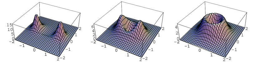
Fig. 1: Two separated lumps (left) approach each other (middle). A ring appears at the coincident limit (right).

A ring structure appears even in finite gauge coupling $(g^{2}<\infty)$ when two semi-local vortices coincide. However the energy density does not exactly vanish and no vacuum appears at the center of the ring unlike the case of the lumps. We show the energy density of two coincident semi-local vortices with various size modulus $|a|$ in the Fig. 2. The energy density at the center of the ring increases as the total size $|a|$ of the semi-local vortices becomes small. This is understood as follows. In the theory with the finite gauge coupling there is the fundamental size $1/(g\sqrt{c})$ which is the size of the ANO vortex as we mentioned above. When the size parameter of the semi-local vortex is much smaller than the ANO size ($|a|\ll 1/(g\sqrt{c})$), the semi-local vortex is almost an ANO vortex. Actually, the configuration with $|a|=0$ is identical with the ANO vortex. On the other hand, the semi-local vortex becomes a lump-like solution with a peak around $|z|\sim|a|$ when $|a|\gg 1/(g\sqrt{c})$. In the limit where the size $|a|$ is taken to infinity, the configuration reduces to the vacuum $H=\sqrt{c}(1,\ 0)$.

Fig. 2: Energy density of two coincident semi-local vortices in the case of $N_{\rm C}=1$ and $N_{\rm F}=2$. The horizontal axis denotes the radius from the coincident point and the vertical axis denotes the energy density. Energy densities with various values of the size modulus $|a|$ are plotted. It has a huge central peak for $a=0$, whereas a central hole with a ring structure develops for larger $|a|$.

2.2 Domain Walls

Let us next turn our attention to the construction of domain walls by using the moduli matrix [41, 42]. Similarly to the BPS vortex in 2+1 dimensions in the previous subsection, we again consider the supersymmetric $U(N_{\rm C})$ gauge theory with eight supercharges. We consider this theory in spacetime dimension 1+1 and turn on the non-degenerate real masses

$$M={\rm diag}\left(m_{1},m_{2},\cdots,m_{N_{\rm F}}\right),\quad\left(m_{A}>m_{A+1}\right)$$ (2.14)

for the $N_{\rm F}(>N_{\rm C})$ hypermultiplets. Due to these hypermultiplet masses, the flavor symmetry $SU(N_{\rm F})$ is explicitly broken to its maximal Abelian subgroup $U(1)^{N_{\rm F}-1}$. The bosonic fields in the vector multiplet are the gauge field $W_{m},(m=0,1)$ and four real adjoint scalars $\Sigma^{I}$ $(I=1,2,3)$ and $\hat{\Sigma}$. We denote $\hat{H}^{i}$ as the hypermultiplet scalars and $(\hat{c},\hat{g})$ as the FI parameter and the gauge coupling in 1+1 dimensions, respectively. Then, the bosonic part of Lagrangian takes the form of

$$\mathcal{L}_{1+1}=\hskip 2.84526pt{\rm Tr}\bigg{[} - \frac{1}{2\hat{g}^{2}}F_{mn}F^{mn}+\frac{1}{\hat{g}^{2}}\mathcal{D}_{m}\Sigma^{I}\mathcal{D}^{m}\Sigma^{I}+\frac{1}{\hat{g}^{2}}\mathcal{D}_{m}\hat{\Sigma}\mathcal{D}^{m}\hat{\Sigma}$$

$$+ \mathcal{D}_{m}\hat{H}^{i}(\mathcal{D}^{m}\hat{H}^{i})^{\dagger}-\frac{1}{2\hat{g}^{2}}[\Sigma^{I},\Sigma^{J}]^{2}-\frac{1}{\hat{g}^{2}}[\Sigma^{I},\hat{\Sigma}]^{2}-\hat{H}^{i}(\hat{H}^{i})^{\dagger}\Sigma^{I}\Sigma^{I}$$

$$+ (\hat{\Sigma}\hat{H}^{i}-\hat{H}^{i}M)(\hat{\Sigma}\hat{H}^{i}-\hat{H}^{i}M)^{\dagger}-\frac{\hat{g}^{2}}{4}(\hat{c}^{a}{\mathbf{1}}_{N_{\rm C}}-(\sigma^{a})^{j}{}_{i}\hat{H}^{i}\hat{H}^{j\dagger})^{2}\bigg{]}.$$ (2.16)

The most points in the vacuum manifold $T^{*}G_{N_{\rm F},N_{\rm C}}$ of the massless theory are lifted by the nondegenerate hypermultiplet masses except for the ${}_{N_{\rm F}}C_{N_{\rm C}}$ discrete points, given by

$$\hat{H}^{1rA}=\sqrt{\hat{c}}\delta^{A}{}_{A_{r}},\hskip 14.22636pt\hat{H}^{2}=\Sigma^{I}=0,\hskip 14.22636pt\hat{\Sigma}={\rm diag}(m_{A_{1}},m_{A_{2}},\cdots,m_{A_{N_{\rm C}}}),$$ (2.17)

where the first equation means that only one flavor component of each (color) row must be non-vanishing. Therefore the vacua are discrete and labeled by sets of the flavors $\langle A_{1},A_{2},\cdots,A_{N_{\rm C}}\rangle$. These are also called color-flavor locking vacua.

The BPS equations for the domain walls interpolating between these discrete vacua are of the form

$$\mathcal{D}_{1}\hat{\Sigma}=\frac{\hat{g}^{2}}{2}(\hat{c}{\mathbf{1}}_{N_{\rm C}}-\hat{H}\hat{H}^{\dagger}),\quad\mathcal{D}_{1}\hat{H}=-\hat{\Sigma}\hat{H}+\hat{H}M.$$ (2.18)

We solve these first order equations by imposing the boundary condition $\langle A_{1},A_{2},\cdots,A_{N_{\rm C}}\rangle$ at $x^{1}=+\infty$ and $\langle B_{1},B_{2},\cdots,B_{N_{\rm C}}\rangle$ at $x^{1}=-\infty$. Here we set $A_{r}\leq B_{r}$, so that $m_{A_{r}}\geq m_{B_{r}}$. The energy of the domain wall is given by the topological charge as

$$T_{\rm w}=\int_{-\infty}^{\infty}dx^{1}\ \hat{c}\ {\rm Tr}(\mathcal{D}_{1}\hat{\Sigma})=\hat{c}[{\rm Tr}\hat{\Sigma}]^{\infty}_{-\infty}=\hat{c}\left(\sum_{k=1}^{N_{\rm C}}m_{A_{k}}-\sum_{k=1}^{N_{\rm C}}m_{B_{k}}\right)>0.$$ (2.19)

As in the case of the vortices, the second equation of (2.18) can be solved by introducing the non-singular $N_{\rm C}\times N_{\rm C}$ matrix $\hat{S}$ and the $N_{\rm C}\times N_{\rm F}$ constant matrix $\hat{H}_{0}$ as [41, 42]

$$\hat{\Sigma}+iW_{1}=\hat{S}^{-1}\partial_{1}\hat{S},\ \ \ \ \hat{H}(x^{1})=\hat{S}^{-1}(x^{1})\hat{H}_{0}e^{Mx^{1}}.$$ (2.20)

We call $\hat{H}_{0}$ the moduli matrix for the domain walls. Notice that $\hat{S}(x^{1})$ depends on $x^{1}$ only while the moduli matrix $\hat{H}_{0}$ is a constant matrix. Defining an $N_{\rm C}\times N_{\rm C}$ gauge invariant matrix

$$\hat{\Omega}(x^{1})=\hat{S}(x^{1})\hat{S}^{\dagger}(x^{1}),$$ (2.21)

the first equation of Eq. (2.18) can be rewritten as [41, 42]

$$\partial_{1}(\partial_{1}\hat{\Omega}\hat{\Omega}^{-1})=\hat{g}^{2}\hat{c}({\mathbf{1}}_{N_{\rm C}}-\hat{\Omega}_{0}\hat{\Omega}^{-1}),\ \ \ \hat{\Omega}_{0}\equiv\frac{1}{\hat{c}}\hat{H}_{0}e^{2Mx^{1}}\hat{H}^{\dagger}_{0},$$ (2.22)

which we call the master equation for domain walls. Once the solution $\hat{\Omega}(x^{1})$ of this equation is obtained, we can calculate all the physical quantities. In the strong gauge coupling limit $g^{2}\to\infty$ this equation reduces to an algebraic equation, which can be solved immediately and uniquely. For finite gauge coupling, uniqueness and existence of the solution of the master equation (2.22) were proved for $N_{\rm C}=1$ [38] and are consistent with the index theorem [44] for arbitrary $N_{\rm C}(<N_{\rm F})$.

The moduli space of the domain walls is obtained by the same way with the vortices. First note that there is the $\hat{V}$-equivalence relation

$$(\hat{H}_{0},\ \hat{S}(x^{1}))\ \sim\ \hat{V}(\hat{H}_{0},\ \hat{S}(x^{1}))$$ (2.23)

where $\hat{V}\in GL(N_{\rm C},{\mathbf{C}})$ is a mere constant matrix. Therefore the total moduli space of BPS domain walls is the complex Grassmannian:

$$\mathcal{M}_{\rm w}\cong\{\hat{H}_{0}|\hat{H}_{0}\sim\hat{V}\hat{H}_{0},\hat{V}\in GL(N_{\rm C},\mathbf{C})\}\cong G_{N_{\rm F},N_{\rm C}}={SU(N_{\rm F})\over SU(N_{\rm F}-N_{\rm C})\times SU(N_{\rm C})\times U(1)}.$$ (2.24)

Since we did not enforce any boundary condition, unlike the one $\det\Omega_{0}={\cal O}(|z|^{2k})$ for vortices, we obtain the total moduli space including all topological sectors connected together properly. We can obtain each topological sector by enforcing a proper boundary condition.

2.3 Scherk-Schwarz dimensional reduction

The massive action in 1+1 dimensions in Sec. 2.2 can be obtained from the massless action in 2+1 dimensions in Sec. 2.1 by the the Scherk-Schwarz (SS) dimensional reduction. In the SS dimensional reduction, the $x^{2}$ direction is compactified on $S^{1}$ with radius $2\pi R\ (\ll 2\pi/m_{A})$ and we impose a twisted boundary condition

$$H^{i}(t,x^{1},x^{2}+2\pi R)=H^{i}(t,x^{1},x^{2})e^{i2\pi RM}.$$ (2.25)

If we ignore the infinite tower of the Kaluza-Klein (KK) modes, we find the hypermultiplet scalar $\hat{H}^{i}(x^{1})$ of 1+1 dimensions in the lightest mode as

$$H^{i}(t,x^{1},x^{2})=\sqrt{\frac{1}{2\pi R}}\hat{H}^{i}(t,x^{1})e^{iMx^{2}}.$$ (2.26)

Furthermore, the lightest (constant) mode of the gauge field $W_{2}$ can be identified with the adjoint scalar $\hat{\Sigma}$ of the vector multiplet in 1+1 dimensions

$$W_{2}(t,x^{1},x^{2})\equiv-\hat{\Sigma}(t,x^{1}).$$ (2.27)

We thus have obtained the 1+1 dimensional Lagrangian (2.16) in Sec. 2.2 from the 2+1 dimensional Lagrangian (2.1) in Sec. 2.1 via the SS dimensional reduction. Both the gauge coupling $\hat{g}$ and the FI parameter $\hat{c}$ in 1+1 dimensions are also related to the corresponding $g$ and $c$ in 2+1 dimensions as

$$\frac{1}{\hat{g}^{2}}=\frac{2\pi R}{g^{2}},\quad\hat{c}=2\pi Rc.$$ (2.28)

By using the above relation (2.26), (2.27) and (2.28), one can easily verify that the BPS equations (2.4) for the vortices reduce to those (2.18) for the domain walls. The topological charge (2.10) of the vortices also reduces to that of the walls in Eq.(2.19), if integrated only over the fundamental region $0\leq x^{2}<2\pi R$. In addition, there is also a relation between the moduli matrix $H_{0}(z)$ for vortices in Eq.(2.5) and $\hat{H}_{0}$ for walls in Eq.(2.20). Taking the relation (2.26) into account, we obtain the relation between the moduli matrices

$$H_{0}(z)\Bigl{|}_{\rm wall}=\hat{H}_{0}e^{Mz}.$$ (2.29)

The meaning of this equation is as follows; When the moduli matrix $H_{0}(z)$ for vortices has the $z$-dependence as in the right hand side, the configurations, generated by $H_{0}(z)$ through Eqs. (2.5) for vortex solutions, become configurations of domain walls. If we restrict the $V$-equivalence relation (2.8) for vortices to preserve the form (2.29), we obtain the $\hat{V}$-equivalence relation (2.23) for domain walls. Therefore, the total moduli space of the vortex ${\cal M}_{\rm v}$ in Eq.(2.9) reduces to that of the domain wall ${\cal M}_{\rm w}$ in Eq.(2.24).

3 Vortices on Cylinder

3.1 Periodically Arranged Vortices

In this section, we construct vortices on $\mathbf{R}\times S^{1}$ by arranging vortices periodically along the $x^{2}$-axis and show that these vortices can split into two wall-like objects as we vary the the moduli parameters. The moduli matrix for periodically arranged vortices is naively given by

$$H_{0}\sim\left(a,\prod_{n=-\infty}^{\infty}(z-z_{0}+i\pi nR)\right),$$ (3.1)

with $a$ being a complex parameter. This moduli matrix corresponds to the configuration in which there exist two vortices in the strip $0<x^{2}<2\pi R$. This is the simplest configuration of the periodically arranged vortices which can be understood as the configuration of the vortices on the cylinder. If we put one vortex in each strip, the configuration will not satisfy the periodic boundary condition $H(x^{1},x^{2})=H(x^{1},x^{2}+2\pi R)$. By using an appropriate regularization method, this moduli matrix can be rewritten as

$$H_{0}=\sqrt{c}\left(\hskip 2.84526pta,\ R\sinh\left(\frac{z-z_{0}}{R}\right)\hskip 5.69054pt\right)\sim\sqrt{c}\left(\hskip 2.84526pt1,\ \frac{R}{a}\sinh\left(\frac{z-z_{0}}{R}\right)\hskip 5.69054pt\right),$$ (3.2)

with $a$ being a complex parameter. In order to see the transition from vortices to wall-like object, it is useful to rewrite this moduli matrix as

$$H_{0}=\sqrt{c}\begin{pmatrix}1,&e^{(z-z_{+})/R}-e^{-(z-z_{-})/R}\end{pmatrix}.$$ (3.3)

where new moduli parameters $z_{+},z_{-}$ are defined as $e^{-z_{+}/R}\equiv(R/2a)e^{-z_{0}/R},\hskip 5.69054pte^{z_{-}/R}\equiv(R/2a)e^{z_{0}/R}$. Namely, $(a,z_{0})$ and $(z_{+},z_{-})$ are good coordinates of moduli for the vortex and the wall-like object respectively to extract physics. The combination of moduli parameters

$${\rm Re}\left(\frac{z_{+}-z_{-}}{R}\right)=2{\rm Re}\left(\log\frac{2a}{R}\right)$$ (3.4)

especially gives the relation between the total size of semi-local vortices and distance for two wall-like objects. The energy density profiles for ${\rm Re}(z_{+}-z_{-})/R<0$, ${\rm Re}(z_{+}-z_{-})/R\approx 0$ and ${\rm Re}(z_{+}-z_{-})/R>0$ in the strong coupling limit are shown in Fig. 3. In the strong coupling limit, the theory reduces to hyper-Kähler nonlinear sigma model on the Higgs branch as its target space. For infinite gauge coupling, the master equation (2.7) becomes a simple algebraic equation and can be solved as $\Omega=\Omega_{0}$. Then we obtain the exact solutions to the BPS equations for vortices (2.4).

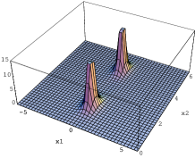
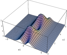
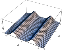
${\rm Re}(z_{+}-z_{-})/R<0$	${\rm Re}(z_{+}-z_{-})/R\approx 0$	${\rm Re}(z_{+}-z_{-})/R>0$

Fig. 3: Energy density of the periodically arranged vortices in the strong coupling limit $g\rightarrow\infty$.

For ${\rm Re}(z_{+}-z_{-})/R<0$ ($2|a|<R$), the energy density profile is just the same as that of two vortices. The sizes of the vortices become larger as we change the moduli parameter ${\rm Re}(z_{+}-z_{-})/R$ to a larger value. For ${\rm Re}\hskip 2.84526pt(z_{+}-z_{-})/R>0$, the vortices split into two wall-like objects, whose positions are given by ${\rm Re}\hskip 2.84526ptz_{+}$ and ${\rm Re}\hskip 2.84526ptz_{-}$. Thus we found that the vortices on $\mathbf{R}\times S^{1}$ can be split into the domain wall-like objects by changing the total scale moduli $a$.

In the case of $\hskip 2.84526pt{\rm Re}(z_{+}-z_{-})/R>0$, the vacua with $H=\sqrt{c}(0,1),\sqrt{c}(1,0),\sqrt{c}(0,1)$ appear in the regions $x^{1}\approx-\infty$, $x^{1}\approx{\rm Re}z_{0}={\rm Re}(z_{+}+z_{-})/2$, $x^{1}\approx\infty$, respectively, and the configurations of large size ($2|a|>R$) vortices on $\mathbf{R}\times S^{1}$ look like a pair of the wall connecting between the vacua $H=\sqrt{c}(0,1),\sqrt{c}(1,0)$ and the anti-wall (not anti BPS) connecting between $H=\sqrt{c}(1,0),\sqrt{c}(0,1)$. An intuitive interpretation of this transition from vortices to walls is as follows: Let us put two vortices on $\mathbf{R}\times S^{1}$ and let the total size of vortices larger than the radius $2\pi R$, the vortices overlap with vortices living in the next fundamental region. Then the overlapping vortices form wall-like objects with a strip of a different vacuum, instead of the ring with a hole for (almost) coincident vortices which was observed in Fig. 1 and Eq.(2.13) in Sec.2.1. In the next section, we will introduce the twisted boundary condition in this system. Then we will obtain deeper understanding of this transition.

3.2 BPS States on Cylinder

In this subsection, we explore the 1/2 BPS states on $\mathbf{R}\times S^{1}$. The action is the same as Sec.2.1 and the only difference here is the twisted boundary condition:

$$H^{i}(x^{1},x^{2}+2\pi R)=H^{i}(x^{1},x^{2})e^{i2\pi RM}$$

$$M\equiv{\rm diag}(m_{1},m_{2},\cdots,m_{N_{\rm F}})$$ .

With this boundary condition, we obtain the 1+1 dimensional theory which admits domain walls if we perform the SS dimensional reduction as we have explained in Sec.2.3. However in this subsection, we take into account all the KK modes. Due to the twisted boundary condition, the vacuum conditions are changed into the following equations:

$$H^{1}(H^{1})^{\dagger}-H^{2}(H^{2})^{\dagger}=c{\mathbf{1}}_{N_{\rm C}},\hskip 14.22636ptH^{1}(H^{2})^{\dagger}=0,$$

$$\Sigma^{I}H^{i}=0,\hskip 14.22636pt[\Sigma^{I},\Sigma^{J}]=0,\hskip 14.22636pt\mathcal{D}_{2}H^{i}=0.\hskip 22.76219pt$$ (3.6)

Compared with the vacuum conditions (2.2) in Sec.2.1, the last equation is added since the hypermultiplet scalars $H^{i}$ cannot be constant due to the twisted boundary condition. Then the vacua is given by

$$H^{1rA}=\sqrt{c}\hskip 2.84526pte^{im_{A_{r}}x^{2}}\delta^{A}{}_{A_{r}},\hskip 11.38109ptH^{2}=\Sigma^{I}=0,$$

$$W_{2}=-{\rm diag}(m_{A_{1}},m_{A_{2}},\cdots,m_{A_{N_{\rm C}}}).\hskip 14.22636pt$$ (3.7)

Therefore, the vacua are discrete and labeled by $\langle A_{1},A_{2},\cdots,A_{N_{\rm C}}\rangle$ as in the case of domain walls. Note that the configurations

$$H^{1rA}=\sqrt{c}\hskip 2.84526pte^{i(m_{A_{r}}+n_{A_{r}}/R)x^{2}}\delta^{A}{}_{A_{r}},\hskip 11.38109ptn_{A_{r}}\in\mathbf{Z},\hskip 11.38109ptH^{2}=\Sigma^{I}=0,$$

$$W_{2}=-{\rm diag}(m_{A_{1}}+n_{A_{1}}/R,\hskip 5.69054ptm_{A_{2}}+n_{A_{2}}/R,\cdots,\hskip 5.69054ptm_{A_{N_{\rm C}}}+n_{A_{N_{\rm C}}}/R)$$ (3.8)

are also vacuum configurations, which are gauge equivalent to the vacua Eq. (3.7) and related by gauge transformations $\Lambda^{r}{}_{s}=\delta^{r}{}_{s}e^{-i(n_{A_{r}}/R)x^{2}}$ which are not connected to the unit element of the gauge group on $\mathbf{R}\times S^{1}$.
The 1/2 BPS equations are the same as in Sec.2.1. Since the moduli matrix $H_{0}(z)$ must satisfy the twisted boundary condition, the components of the moduli matrix can be written as

$$H_{0}^{rA}(z)=e^{m_{A}z}\sum_{n=-\infty}^{\infty}a^{rA}_{n}e^{nz/R}=u^{m_{A}R}\sum_{n=-\infty}^{\infty}a^{rA}_{n}u^{n},\hskip 14.22636ptu\equiv e^{z/R},$$ (3.9)

namely polynomials of $u$ and $u^{-1}$ with the factors $u^{m_{A}R}$. For a configuration which interpolates two vacua $\langle A_{1},A_{2},\cdots,A_{N_{\rm C}}\rangle$ and $\langle B_{1},B_{2},\cdots,B_{N_{\rm C}}\rangle$, the topological charge $\tilde{k}$ is given by

$$\tilde{k} = \frac{1}{2\pi}\int_{-\infty}^{\infty}dx^{1}\int_{0}^{2\pi R}dx^{2}{\rm Tr}F_{12}$$ (3.10)

$$= \frac{1}{4\pi}\left(\int_{0}^{2\pi R}dx^{2}\partial_{1}\log\det\Omega_{0}\Big{|}_{x^{1}=\infty}-\int_{0}^{2\pi R}dx^{2}\partial_{1}\log\det\Omega_{0}\Big{|}_{x^{1}=-\infty}\right)$$

$$= k+R\Bigl{(}\sum_{r=1}^{N_{\rm C}}m_{A_{r}}-\sum_{r=1}^{N_{\rm C}}m_{B_{r}}\Bigl{)},\hskip 28.45274ptk\in{\mathbf{Z}}.$$

Therefore the highest power of $|u|^{2}$ minus the lowest power of $|u|^{2}$ in $\det\Omega_{0}$ gives the topological charge. The term $R\Bigl{(}\sum_{r=1}^{N_{\rm C}}m_{A_{r}}-\sum_{r=1}^{N_{\rm C}}m_{B_{r}}\Bigl{)}$ appears because of the twisted boundary condition and gives the fractional topological charge. We will see later that the integer $k$ gives the number of vortices and the fractional topological charge corresponds to the tension of domain wall. Then the moduli space of the solutions with topological charge $\tilde{k}$ is expressed as

$$\mathcal{M}^{\tilde{k}}_{v}\cong\mathcal{G}/\sim,$$

$$\mathcal{G}\equiv\Bigg{\{}H_{0}\hskip 5.69054pt\bigg{|}\hskip 5.69054ptH_{0}:\mathbf{R}\times S^{1}\rightarrow M(N_{\rm C}\times N_{\rm F},\mathbf{C}),\hskip 5.69054pt\overline{\partial}_{z}H_{0}=0,$$

$$\hskip 71.13188pt\det\Omega_{0}\xrightarrow[x^{1}\to\infty]{}|u|^{2l},\hskip 5.69054pt\det\Omega_{0}\xrightarrow[x^{1}\to-\infty]{}|u|^{2\tilde{l}},\hskip 5.69054ptl-\tilde{l}=\tilde{k}\Bigg{\}}$$

$$H_{0}(z)\sim V(z)H_{0}(z),\hskip 14.22636ptV(z)\in GL(N_{\rm C},\mathbf{C}),\hskip 14.22636pt\overline{\partial}_{z}V(z)=0,$$

where again note that all fields appearing in the above equations have to satisfy the twisted boundary condition.
Next we will give the useful estimation method for the $x^{1}$-positions of vortices and walls. By using this method, we can investigate the transition between walls and vortices in general. The energy density can be roughly estimated as follows:

$${\cal E} = c\hskip 2.84526pt\partial_{z}\bar{\partial}_{z}\log\det\Omega\simeq c\hskip 2.84526pt\partial_{z}\bar{\partial}_{z}\log\det\Omega_{0}$$

$$\det\Omega_{0} = \det\Bigl{(}\frac{1}{c}H_{0}H_{0}^{\dagger}\Bigl{)}=\sum_{\langle A\rangle}\Bigl{|}\det\frac{1}{\sqrt{c}}H_{0\langle A\rangle}\Bigl{|}^{2}$$

where $\langle A\rangle\equiv\langle A_{1}\cdots A_{\rm N_{\rm C}}\rangle$ is the $N_{\rm C}$ set of flavors and the $(r,s)$ component of $N_{\rm C}\times N_{\rm C}$ matrix $H_{0\langle A\rangle}$ is given by $(H_{0})^{rA_{s}}$. Now, it is useful to introduce linear holomorphic functions $f_{\langle A\rangle}^{n}(z)$ as

$$\det\left(\frac{1}{\sqrt{c}}H_{0\langle A\rangle}\right)=\sum_{n}e^{f_{\langle A\rangle}^{n}},\ \ \ \ f_{\langle A\rangle}^{n}\equiv\Bigl{(}\frac{n}{R}+\sum_{r=1}^{N_{C}}m_{A_{r}}\Bigl{)}z+s_{{\langle A\rangle}}$$

where the $s_{{\langle A\rangle}}$ are some functions of moduli parameters. If there is the region where only one of $e^{f_{\langle A\rangle}^{n}}$ is dominant in $\det\Omega_{0}$, the energy density vanish there because $\partial\bar{\partial}\log|\sum e^{f_{\langle A\rangle}^{n}}|^{2}=0$. In contrast, if there is the region where the two of $e^{f_{\langle A\rangle}^{n}}$ are comparable, the energy density is non-vanishing. Therefore, there exist walls or vortices in the region where ${\rm Re}f_{\langle A\rangle}^{n}\approx{\rm Re}f_{\langle B\rangle}^{m}$. Since the functions $f_{\langle A\rangle}^{n}$ are linear in $z$, the energy density at the transition point ${\rm Re}f_{\langle A\rangle}^{n}={\rm Re}f_{\langle B\rangle}^{m}\ (A\not=B)$ is independent of $x^{2}$, so that there is the wall $\langle A\to B\rangle$ at this point. On the other hand, there are $k$-vortices at the transition point ${\rm Re}f_{\langle A\rangle}^{n}={\rm Re}f_{\langle A\rangle}^{m}\ (n-m=k)$.

We now see some explicit examples in the case of $N_{\rm C}=1,\hskip 5.69054ptN_{\rm F}=2$. First, we consider $k=0$ case. The most general moduli matrix is given by

$$H_{0}=\sqrt{c}\begin{pmatrix}1,&a\end{pmatrix}e^{Mz}=\sqrt{c}\begin{pmatrix}1,&a\end{pmatrix}\begin{pmatrix}u^{m_{1}R}&0\\ 0&u^{m_{2}R}\end{pmatrix},$$ (3.12)

where $a$ is a complex parameter. For this moduli matrix, there are no contributions from the KK modes to any physical quantities. Therefore this moduli matrix corresponds to the domain wall configuration as stated in Sec.2.3.
Next, we investigate $\tilde{k}=1$ case. This is the simplest case where KK-modes contribute to the topological charge. The moduli matrix is given by

$$H_{0}=\sqrt{c}\begin{pmatrix}a_{1},&e^{z/R}+a_{2}\end{pmatrix}e^{Mz}\sim\sqrt{c}\begin{pmatrix}1,&\frac{1}{a_{1}}(u+a_{2})\end{pmatrix}\begin{pmatrix}u^{m_{1}R}&0\\ 0&u^{m_{2}R}\end{pmatrix}$$ (3.13)

$$a_{1}\in\mathbf{C},\hskip 14.22636pta_{2}\in\mathbf{C}-\{0\}.$$

Note that in the strong coupling limit, the master equation (2.7) can be solved as $\Omega=\Omega_{0}=\frac{1}{c}H_{0}H_{0}^{\dagger}$. Therefore, the energy density for this moduli matrix in the strong coupling limit can be expressed as

$$\mathcal{E}(x^{1},x^{2}) = c\hskip 2.84526pt\partial_{z}\bar{\partial}_{z}\log\left(|e^{f_{\langle 1\rangle}^{0}}|^{2}+|e^{f_{\langle 2\rangle}^{1}}+e^{f_{\langle 2\rangle}^{0}}|^{2}\right),$$ (3.14)

where we have defined the functions $f_{\langle A\rangle}^{n}$, which are linear in $z$, by

$$f^{0}_{\langle 1\rangle}(z)=m_{1}z,\hskip 99.58464pt$$

$$f^{0}_{\langle 2\rangle}(z)=m_{2}z+\log\frac{a_{2}}{a_{1}},\hskip 14.22636ptf^{1}_{\langle 2\rangle}(z)=\left(\frac{1}{R}+m_{2}\right)z-\log a_{1}.$$ (3.15)

Now we will explain the fact that one vortex can be decomposed into two walls by changing the scale moduli. We begin with the region in the moduli space where the profiles of the functions $f_{\langle A\rangle}^{n}$ are like Fig. 4(i)-(a). We can see that there exist one vortex at the transition point where $f_{\langle 2\rangle}^{0}=f_{\langle 2\rangle}^{1}$. Next, let us change the scale moduli $a_{1}$ to a larger value and consider the case where the profiles of the functions $f_{\langle A\rangle}^{n}$ are like Fig. 4(i)-(b). In this region of moduli space, two walls appear at two transition points; $f_{\langle 2\rangle}^{0}=f_{\langle 1\rangle}^{0}$ and $f_{\langle 1\rangle}^{0}=f_{\langle 2\rangle}^{1}$. The corresponding energy density are shown in Fig. 4(ii)-(a),(b). Therefore we can conclude that one vortex can be decomposed into the wall $\langle 0\to 1\rangle$ and the anti wall $\langle 1\to 0\rangle$ by changing the scale moduli parameter.

Now we return to Sec.3.1 and comment on the relation between the twisted boundary condition and the periodic one. If we turn off the the parameters $m_{i}$, we may well deduce that the former reduces to the latter. In this limit, however, we have to take into account the periodic boundary condition because that some of $f_{\langle A\rangle}^{n}$ belonging to the same flavor reduce to have the same slope. As a result, we need at least two vortices at the same $x^{1}$ point in the fundamental region. Except for this technical point, whole argument are essentially the same as in the twisted one. For ${\rm Re}(z_{+}-z_{-})<0$, since the configuration is the same vacuum configuration in the region where ${\rm Re}\hskip 2.84526ptz\ll{\rm Re}z_{0}={\rm Re}(z_{+}+z_{-})/2$ and ${\rm Re}\hskip 2.84526ptz\gg{\rm Re}z_{0}$, the vortices appear at ${\rm Re}\hskip 2.84526ptz={\rm Re}z_{0}$. For ${\rm Re}(z_{+}-z_{-})>0$, the configuration approaches the vacuum $H=\sqrt{c}(0,1)$ at ${\rm Re}\hskip 2.84526ptz\rightarrow\pm\infty$ and $H\approx\sqrt{c}(1,0)$ in the region where ${\rm Re}\hskip 2.84526ptz_{-}<{\rm Re}\hskip 2.84526ptz<{\rm Re}\hskip 2.84526ptz_{+}$. Since there are two transition points of the different vacua, two walls appear at $z=z_{+}$ and $z=z_{-}$.

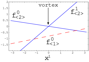
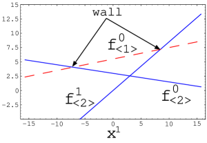
(a) vortex	(b)two walls
(i) Comparison of the functions $f_{A}^{n}$
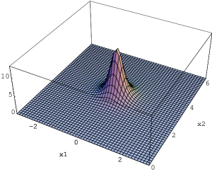
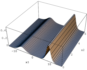
(a)	(b)
(ii) Energy density
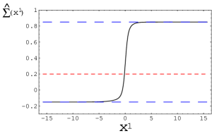
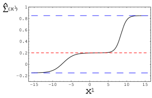
(a)	(b)
(iii) vector multiplet scalar $\Sigma(x^{1})$

Fig. 4: Examples: $R=1,\hskip 5.69054ptm_{1}=0.2,\hskip 5.69054ptm_{2}=-0.15$      (a) $a_{1}=e^{-0.6},a_{2}=1$, (b) $a_{1}=e^{5.5},a_{2}=e^{3}$

Next we calculate the Wilson loops around the $S^{1}$ of the cylinder and relate this to $\hat{\Sigma}(x^{1})$ by

$$\hat{\Sigma}(x^{1})\equiv-\frac{1}{2\pi R}\log\Bigl{[}\mathbf{P}\ {\rm exp}\int_{0}^{2\pi R}dx^{2}W_{2}(x_{1},x_{2})\Bigl{]}.$$ (3.16)

If the gauge field $W_{2}$ is independent of $x^{2}$, the definition of $\hat{\Sigma}(x^{1})$ in Eq. (3.16) reduces to the one in Eq. (2.27). Therefore this quantity corresponds to the scalar field in the vector multiplet after the dimensional reduction. In general $\hat{\Sigma}(x^{1})$ exhibits kinks as seen below. To illustrate this we consider the case of $N_{\rm C}=1,\hskip 5.69054ptN_{\rm F}=2$ and $\tilde{k}=1$. We take the strong gauge coupling limit $g\rightarrow\infty$ for simplicity. Then the gauge field can be obtained explicitly as

$$W_{2}=-S^{-1}\partial_{1}S,\hskip 14.22636ptS=\sqrt{H_{0}H_{0}^{\dagger}\over c},$$ (3.17)

with $H_{0}$ given in Eq. (3.13). Then, we obtain $\hat{\Sigma}(x^{1})$ by integrating the gauge field around $S^{1}$:

$$\hat{\Sigma}(x^{1}) = -\frac{1}{2\pi R}\int_{0}^{2\pi R}dx^{2}W_{2}(x^{1},x^{2})$$

$$= \frac{|a_{1}|^{2}(m_{1}-m_{2}-\frac{1}{2R})e^{2m_{1}x^{1}}+\frac{1}{2R}(e^{2x^{1}/R}-|a_{2}|^{2})e^{2m_{2}x^{1}}}{\sqrt{(e^{2(m_{2}+1/R)x^{1}}+|a_{1}|^{2}e^{2m_{1}x^{1}}+|a_{2}|^{2}e^{2m_{2}x^{1}})^{2}-4|a_{2}|^{2}e^{2(2m_{2}+1/R)x^{1}}}}$$

$$+m_{2}+\frac{1}{2R},$$

Fig. 4(iii) (a),(b) show examples of the vector multiplet scalar $\hat{\Sigma}(x^{1})$.

Although in the small size limit $|a_{1}|\rightarrow 0$ the semi-local vortex reduces to the ANO vortex for a finite gauge coupling constant, it corresponds to small lump singularity in the strong coupling limit. Correspondingly, as shown in the Fig. 5, $\hat{\Sigma}(x^{1})$ becomes a step function in the small size limit $|a_{1}|\rightarrow 0$:

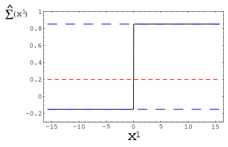
Fig. 5: Profile of small size limit of $\hat{\Sigma}(x^{1})$ in the strong gauge coupling limit

$$\hat{\Sigma}(x^{1}) \rightarrow \frac{1}{2R}\frac{(e^{2x^{1}/R}-|a_{2}|^{2})e^{2m_{2}x^{1}}}{\sqrt{((e^{2x^{1}/R}-|a_{2}|^{2})e^{2m_{2}x^{1}})^{2}}}+m_{2}+\frac{1}{2R}$$ (3.19)

$$= \frac{1}{2R}{\rm sign}\left(x^{1}-\frac{R}{2}\log|a_{2}|^{2}\right)+m_{2}+\frac{1}{2R}.$$

This result reflects the fact that the size of the vortex is encoded to the size of kink of $\hat{\Sigma}(x^{1})$. In the next section, we discuss the brane construction of our model. In the brane construction, our theory corresponds to the worldvolume theory of the D3 branes. After taking the T-duality transformation, $\hat{\Sigma}(x^{1})$ parameterizes the position of the D2 branes in the dual direction. Therefore $\hat{\Sigma}(x^{1})$ can be understood as the position of D-branes in the dual direction.

Next we consider $R\rightarrow 0$ limit and show that the finite energy solutions are ordinary domain wall solutions after taking the limit. When we take the limit, we keep both the FI parameter $\hat{c}$ and the masses $m_{A}$ in the (1+1)-dimension fixed. We again use the moduli matrix in Eq. (3.13) as an example. If $a_{1}$ is small, the corresponding configuration is a one vortex configuration. Since the mass of the vortex is $2\pi c=\frac{\hat{c}}{R}$, the vortex decouples in the $R\rightarrow 0$ limit. If the parameter $a_{1}$ is sufficiently large, there are two walls with masses $2\pi cR(m_{1}-m_{2})=\hat{c}(m_{1}-m_{2})$ and $2\pi c(1-R(m_{1}-m_{2}))=\hat{c}(\frac{1}{R}-(m_{1}-m_{2}))$. The wall with mass $\hat{c}(m_{1}-m_{2})$ is the ordinary domain wall appearing in the (1+1)-dimensional theory. The other wall with mass $\hat{c}(\frac{1}{R}-(m_{1}-m_{2}))$ becomes infinitely massive. To obtain a meaningful limit $R\rightarrow 0$, we need to let the position of this infinitely massive wall to either infinity $x^{1}\rightarrow\pm\infty$. In this sense, this infinitely massive wall decouples. In the case of $\tilde{k}=k+R(m_{1}-m_{2})\geq 1$ for $k=1$, an additional domain wall with mass $\hat{c}(m_{1}-m_{2})$ exists. However, one should note that the walls are inevitably ordered in such a way that the infinitely massive wall is sandwiched between this wall and the previously mentioned wall with the same mass $\hat{c}(m_{1}-m_{2})$. Therefore either one of the two walls with the mass $\hat{c}(m_{1}-m_{2})$ must go to infinity in the $R\rightarrow 0$ limit, since it should be outside of the infinitely massive wall which goes to infinity in the limit. For arbitrary $N_{\rm C}$ and $N_{\rm F}$ there are $N_{\rm F}$ kinds of domain walls and one of these walls has mass which will be infinite in the $R\rightarrow 0$. For a finite $R$, the numbers of the $N_{\rm F}$ types walls are not restricted. However, as in the case of the previous example, the infinitely massive walls take some of the other walls to the infinity in the $R\rightarrow 0$ limit. For a finite energy solution, at most $(N_{\rm F}-N_{\rm C})\times N_{\rm C}$ walls are left in the $R\rightarrow 0$ limit and these are the ordinary domain walls appearing in the (1+1)-dimensional theory.

4 Brane Configurations and T-duality

In this section, we discuss the relation between vortices and domain walls by using the brane configurations. First we consider a brane configuration for vortices [15, 17]. Fig. 6 shows the brane configuration for vortices and Table 1 shows the directions in which the branes extend.

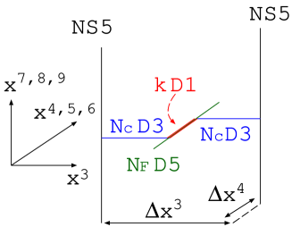
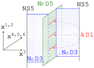
Fig. 6: Brane configuration for $k$ vortices

	$x^{0}$	$x^{1}$	$x^{2}$	$x^{3}$	$x^{4}$	$x^{5}$	$x^{6}$	$x^{7}$	$x^{8}$	$x^{9}$
$N_{\rm C}$ $\rm D3$	$\circ$	$\circ$	$\circ$	$\circ$	$-$	$-$	$-$	$-$	$-$	$-$
$N_{\rm F}$ $\rm D5$	$\circ$	$\circ$	$\circ$	$-$	$\circ$	$\circ$	$\circ$	$-$	$-$	$-$
$2\hskip 5.69054pt{\rm NS}5$	$\circ$	$\circ$	$\circ$	$-$	$-$	$-$	$-$	$\circ$	$\circ$	$\circ$
$k\hskip 5.69054pt\rm D1$	$\circ$	$\times$	$\times$	$-$	$\circ$	$-$	$-$	$-$	$-$	$-$

Table 1: Brane configuration for $k$ vortices: Branes are extended along directions denoted by $\circ$, and are not extended along directions denoted by $-$. The symbol $\times$ denotes the codimensions of the k D1-branes on the worldvolume of the D3-branes excluding the $x^{3}$ which is a finite line segment.

Since the coincident $N_{\rm C}$ $\rm D3$ branes which are stretched between two ${\rm NS}5$ branes have the finite length $\Delta x^{3}$, the theory on the worldvolume of the $\rm D3$ branes reduces to $(2+1)$-dimensional $U(N_{\rm C})$ gauge theory with a gauge coupling $\frac{1}{g^{2}}=|\Delta x^{3}|\tau_{3}l_{s}^{4}=\frac{|\Delta x^{3}|}{g^{(B)}_{s}}$, where $g^{(B)}_{s}$ is the string coupling constant in type IIB string theory and $\tau_{3}=1/g^{(B)}_{s}l_{s}^{4}$ is the D3-brane tension. Since the positions of the $N_{\rm F}$ $\rm D5$ branes in the $x^{7}$-,$x^{8}$- and $x^{9}$-directions coincide with those of the $\rm D3$ branes, the $N_{\rm F}$ hypermultiplets in the D3 brane worldvolume theory coming from D3-D5 strings are massless. The separations of two ${\rm NS}5$ branes in the $x^{4}$-,$x^{5}$- and $x^{6}$-directions correspond to the triplet of the FI parameters $c^{a}$, which we choose as $c^{a}=(0,0,c=\Delta x^{4}/g^{(B)}_{s}l_{s}^{2}>0)$, where $l_{s}$ is the string length. The symbol $\times$ in Table 1 denotes the codimensions of the $k\hskip 5.69054pt\rm D1$ branes on the worldvolume of the $\rm D3$ branes. Since the $x^{3}$ direction of the $\rm D3$ brane worldvolume is a finite line segment, the $\rm D1$ branes are interpreted as codimension-two objects on the $\rm D3$ branes. Moreover, the energy $\tau_{1}\Delta x^{4}=\frac{\Delta x^{4}}{g^{(B)}_{s}l_{s}^{2}}=c$ of each $\rm D1$ brane corresponds to the energy of a vortex given in Eq.(2.10). Therefore the $k\hskip 5.69054pt\rm D1$ branes correspond to $k$ vortices in the $\rm D3$ brane worldvolume theory.

Next, we consider the T-dual picture of this configuration. We compactify the $x^{2}$ direction on $S^{1}$ with radius $R$ and take T-duality along that direction. Table 2 shows the directions in which the branes extend after T-duality transformation.

	$x^{0}$	$x^{1}$	$x^{2}$	$x^{3}$	$x^{4}$	$x^{5}$	$x^{6}$	$x^{7}$	$x^{8}$	$x^{9}$
$N_{\rm C}$ $\rm D2$	$\circ$	$\circ$	$-$	$\circ$	$-$	$-$	$-$	$-$	$-$	$-$
$N_{\rm F}$ $\rm D4$	$\circ$	$\circ$	$-$	$-$	$\circ$	$\circ$	$\circ$	$-$	$-$	$-$
$2\hskip 5.69054pt{\rm NS}5$	$\circ$	$\circ$	$\circ$	$-$	$-$	$-$	$-$	$\circ$	$\circ$	$\circ$
$k\hskip 5.69054pt\rm D2^{\prime}$	$\circ$	$\times$	$\circ$	$-$	$\circ$	$-$	$-$	$-$	$-$	$-$

Table 2: T-dualized configuration: Branes are extended along directions denoted by $\circ$, and are not extended along directions denoted by $-$. The symbol $\times$ denotes the codimensions of the k D2’-branes on the worldvolume of the D2-branes, excluding the $x^{3}$ which is a finite line segment.

Before T-dualizing, we turn on a constant background gauge field $A_{2}={\rm diag}(m_{1},\cdots,m_{N_{\rm F}})$ on the $\rm D5$ brane worldvolume, that is a non-trivial Wilson loop around $S^{1}$ on the $\rm D5$ branes. With this Wilson loop, the resulting $\rm D4$ branes split in the $x^{2}$-direction and their positions are determined as $X^{2}_{A}=2\pi l_{s}^{2}m_{A}\hskip 5.69054pt(A=1,\cdots,N_{\rm F})$. These separations give hypermultiplet masses in the $\rm D2$ brane worldvolume theory. The worldvolume theory of the $\rm D2$ branes is $(1+1)$-dimensional gauge theory with a gauge coupling $\frac{1}{\hat{g}^{2}}=\frac{\Delta x^{3}l_{s}}{g^{(A)}_{s}}=\frac{\Delta x^{3}R}{g^{(B)}_{s}}$ and the FI parameter $\hat{c}=\frac{\Delta x^{4}}{g^{(A)}_{s}l_{s}}=\frac{\Delta x^{4}R}{g^{(B)}_{s}l^{2}_{s}}$, where $g^{(A)}_{s}$ is the string coupling constant in type IIA string theory.

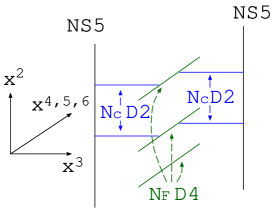
Fig. 7: vacuum configuration $(k=0)$

For $k=0$, as shown in Fig. 7, each $\rm D2$ brane ends on one of the $\rm D4$ branes and at most one $\rm D2$ brane can be stretched between a $\rm D4$ brane and a ${\rm NS5}$ brane due to the s-rule [57]. These configurations correspond to the vacua in the $\rm D2$ brane worldvolume theory.

For $k\not=0$, the $\rm D1$ branes transform into $\rm D2$ branes stretched between the $\rm D4$ branes and we denote these $\rm D2$ branes as $\rm D2^{\prime}$.

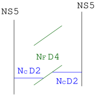
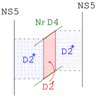
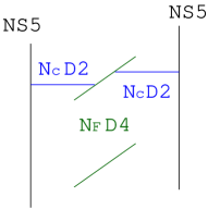
	$x^{1}=-\infty$	$x^{1}=x_{0}$	$x^{1}=+\infty$

Fig. 8: T-dualized configurations for $k=1$: the $\rm D2^{\prime}$ brane is assumed to be located at $x^{1}=x_{0}$.

Fig. 8 shows the brane configurations for $k=1$. Since the $\rm D2$ branes are attached to different $\rm D4$ branes at $x=-\infty$ and $x=+\infty$, there must exist $\rm D2$ branes which connect the $\rm D2$ branes ending on different $\rm D4$ branes. These $\rm D2$ branes correspond to $\rm D2^{\prime}$ in Fig. 8 and Fig. 9. In addition, there must be $\rm D2$ branes ($\rm D2^{\ast}$ in Fig. 8 and Fig. 9) at a points where the $\rm D2^{\prime}$ branes are located and the $\rm D2^{\prime}$ branes end on these $\rm D2^{\ast}$ branes. Fig. 9 shows the resulting brane configuration for $k=1$ which corresponds to a BPS domain wall configuration in the $\rm D2$ brane theory. Indeed, we can easily calculate the energy of the domain walls from this brane configuration in the strong coupling limit. Since the gauge coupling $\frac{1}{\hat{g}^{2}}$ is proportional to $\Delta x^{3}$, the $\rm D2^{\ast}$ branes disappear in the limit $\hat{g}\rightarrow\infty$. The remaining $\rm D2^{\prime}$ branes have the energy $\tau_{2}\hskip 2.84526pt\Delta x^{4}\hskip 2.84526ptl_{s}^{2}\Delta m=\frac{\Delta x^{4}\Delta m}{g^{(A)}_{s}l_{s}}=\hat{c}\hskip 2.84526pt\Delta m$ and this corresponds to the energy (2.19) of a domain wall.

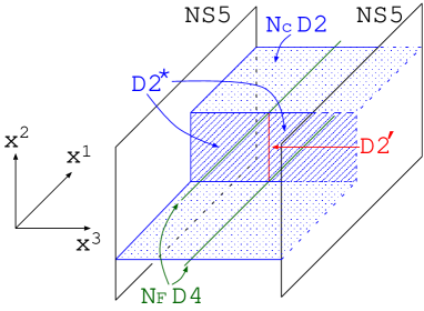
Fig. 9: Brane configuration for a wall

We thus conclude that the vortices and the domain walls are related by T-duality. This relation is analogous to the relation between instantons and monopoles. In Fig. 6 the ${\rm D}1$ branes, which correspond to the vortices in the $\rm D3$ brane worldvolume theory, can be thought of as instantons in the $\rm D5$ brane worldvolume theory. Similarly, the $\rm D2^{\prime}$ brane in the Fig. 9 can be thought of as a monopole in the $\rm D4$ brane worldvolume theory. For this reason, the relation between vortices and domain walls is similar to the relation between instantons and monopoles.

Before taking T-duality, D1-brane end-points on D3-branes (in Fig. 6-(b)) are not actually points with zero size from the point of view of the field theory on the D3 branes. Instead, they have the vortex size $1/g\sqrt{c}$ (or lager size in the case of semi-local vortices). This actual configuration can be read from gauge fields. Correspondingly, this information is expected to be mapped into the Wilson loop by taking T-duality. In fact, although we have naively assumed the positions of the $\rm D2$ branes in the $x^{2}$ direction so far in this section, the actual positions of the D-branes must be parameterized by $\hat{\Sigma}(x^{1})$ Eq. (3.16). We have already calculated $\hat{\Sigma}(x^{1})$ in Sec.3.2 for $N_{\rm F}=2,N_{\rm C}=1,k=1$ as in Eq. (3.2), and have found that the vortex configuration shown in Fig. 4 (a) [for (i) - (iii)] interpolates the same vacuum. In the brane picture, the vortex corresponds to the D2 brane winding around the $S^{1}$ of the cylinder with exhibiting a kink as in Fig. 10 (a). The size of this kink in $x^{1}$ is the ANO vortex size $1/g\sqrt{c}$ from the construction. Note that the scalar field $\hat{\Sigma}(x^{1})$ has period $1/R$.

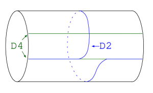
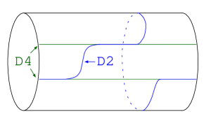
	(a)	(b)

Fig. 10: T-dual picture for $N_{\rm F}=2,N_{\rm C}=1,k=1$.

This vortex can be decomposed into two walls by changing the size of the vortex as in Fig. 4 (b) [for (i) - (iii)]. In this configuration, the D2 brane is attached to the same D4 brane at $x^{1}\rightarrow\pm\infty$ with exhibiting kinks twice as in Fig. 10 (b). In the middle region, the D2 brane ends on the other D4 brane. Therefore, there are two walls at the points where the D2 brane change the D4 brane to end on. Interestingly, the relative distance between two kinks corresponds to the size moduli of the single semi-local vortex. Moreover we can easily understand the small size limit of the configuration reduces to the ANO vortex with the ANO size $1/g\sqrt{c}$. Small lump singularity in the strong coupling limit $g\to\infty$ is resolved by the size of the ANO vortex for finite $g$, as discussed in Eq. (3.19). This example suggests the possibility to understand all moduli of vortices solely by kinky configurations, like Fig. 10. We show that this is the case in the next section.

Before going that we make a comment. Taking T-duality further along the $x^{3}$-direction after compactifying that direction, the system is mapped to D1-D5 system where two NS5-branes are mapped to the asymptotically locally Euclidean (ALE) geometry with ${\bf Z}_{2}$ singularity resolved by the string scale [45]. (The four directions of D5 brane worldvolume perpendicular to D1 branes are divided by this ${\bf Z}_{2}$.) In that brane configuration, D1 branes (instead of D2 branes in Fig. 10) exhibit kinks interpolating separated D5 branes (instead of D4 branes in Fig. 10). In the discussion in the next section, we may consider either the D2-D4-NS5 system or the D1-D5-ALE system.

5 Moduli Space of Vortices from Kinky D-branes

In this section, we explore the relation between the moduli spaces of vortices and domain walls. In our previous paper [45] we realized domain walls in non-Abelian gauge theory by a kinky D-brane configuration. We would like to describe the moduli space of vortices on a cylinder without twisted boundary condition. However we put small mass splitting $m_{A}$ and analyze moduli in kinky D-branes after taking a T-duality along $S^{1}$. One advantage to do so is that the internal moduli of vortices, like orientational moduli of non-Abelian vortices, become visible. We also obtain the moduli space of vortices on a plane ${\bf C}$, by taking the limit $\hat{R}\to 0$ of shrinking dual circle.

5.1 Dimensionality

First of all we discuss dimensionality of the moduli spaces. It is known that the dimension of the moduli space of the $k$ vortices is $2kN_{\rm F}$ for arbitrary $N_{\rm C}(\leq N_{\rm F})$ [15]. We now show that this can be seen from the T-dual picture of the vortex configurations. The T-dual picture of the one vortex configuration is given in Fig. 11. This brane configuration can be decomposed into kinky D-branes exhibiting small kinks $N_{\rm F}-1$ times and one large kink. They represent $N_{\rm F}-1$ light walls and a heavy wall, respectively.

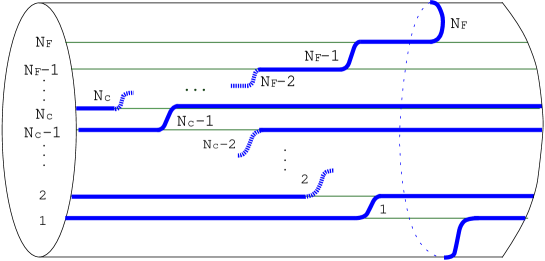
Fig. 11: Brane configuration for one vortex.

Each wall have the two moduli parameters: one is for the position of walls and the other is for the phase. Therefore the dimension of the moduli space of one vortex is $2N_{\rm F}$.

The T-dual picture of the $k$ vortices contains $k$ units of one vortex configuration as shown in Fig. 12.

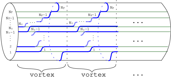
Fig. 12: Brane configuration for $k$ vortex.

In this brane configuration, there are $kN_{\rm F}$ walls and thus we conclude that the dimension of the moduli space is $2kN_{\rm F}$.

We also find non-normalizable zero modes from these figures. In the limit of $m_{A}\to 0$ (without the twisted boundary condition), all D4 branes coincide and the moduli $G_{N_{\rm F},N_{\rm C}}\simeq SU(N_{\rm F})/[SU(N_{\rm F}-N_{\rm C})\times SU(N_{\rm C})\times U(1)]$ appear at both infinities of $x^{1}\to\pm\infty$ from the freedom of D2-branes on D4-branes and become non-normalizable.

5.2 Single non-Abelian vortex from kinky branes

Next, we explore more concrete relations between the moduli spaces of vortices and walls. First, let us discuss a single vortex moduli space in the case of $N_{\rm F}=N_{\rm C}=2$.

The moduli matrix for this case on ${\bf C}$ is given by [24]

$$H_{0}=\begin{pmatrix}1&b\\ 0&u-u_{0}\end{pmatrix}\hskip 14.22636ptb,u_{0}\in\mathbf{C}\hskip 14.22636ptu_{0}\not=0.$$ (5.1)

By using the $V$-equivalence relation (2.8), it can also be written as

$$H_{0}=\begin{pmatrix}u-u_{0}&0\\ \tilde{b}&1\end{pmatrix}\hskip 14.22636pt\tilde{b}=\frac{1}{b}.$$ (5.2)

The moduli parameter $u_{0}$ corresponds to the position of the vortex. The parameters $b$ and $\tilde{b}$ are the inhomogeneous coordinates of $\mathbf{C}P^{1}$. We thus have ${\bf C}\times{\bf C}P^{1}$ as found earlier in [16]. For $N_{\rm F}=N_{\rm C}=2$, the moduli space of one vortex on the cylinder $\mathbf{R}\times S^{1}$ is given by

$$\mathcal{M}_{N_{\rm C}=N_{\rm F}=2}^{k=1}={\mathbf{C}}^{*}\times\mathbf{C}P^{1}$$ (5.3)

with ${\bf C}^{*}\equiv{\bf C}-\{0\}\simeq{\bf R}\times S^{1}$.

Let us see this moduli space in terms of the T-dual picture. The brane configuration for the T-dual picture is given in Fig. 13. There are two walls in this configuration and each wall has two moduli parameters. The position and the phase of the larger wall correspond to the position of the vortex in the $x^{1}$ direction and $x^{2}$ direction, respectively. The smaller wall also has two moduli parameters, that is the position and the phase. However, the position of this wall is confined inside the larger kink from the both sides, and hence the position modulus becomes a line segment. At the boundaries of that line segment, the D2 branes are reconnected [45]. As a result we obtain a single D2 brane winding once and a straight D2 brane as shown in Fig. 14. Therefore the phase degree of freedom of the smaller wall disappears at the boundaries. We thus have $\mathbf{C}P^{1}$ from the moduli parameters of the smaller wall, reproducing the orientational moduli $\mathbf{C}P^{1}$ in the moduli space of the single vortex, given in Eq. (5.3).

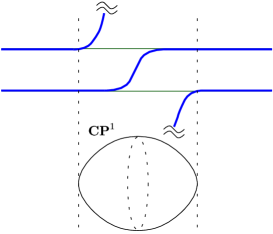
Fig. 13: Brane configuration for one vortex

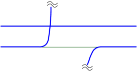
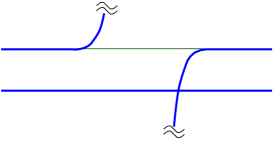
(a) $b=0$ ($I=+1$)	(b) $\tilde{b}=0$ ($I=-1$)

Fig. 14: The $b=0$ and $\tilde{b}=0$ limits.

Interestingly the winding D2 brane represents the ANO vortex.

For later convenience we introduce the intersecting number $I$ of kinky D-brane configuration [45]. When there exist no crossing D2 branes we define $I=0$. When reconnection occurs once it becomes $I=\pm 1$ with the sign depending on which brane goes across which brane. If the straight-going upper (lower) D2-brane in the left side crosses over the lower (upper) D2-brane we define $I=-1$ ($I=+1$). The configurations in Fig. 14 (a) and (b) have $I=+1$ and $I=-1$, respectively.

The generalization to a single vortex moduli space for arbitrary $N\equiv N_{\rm C}=N_{\rm F}$ is straightforward. Fig. 15 shows the brane configuration for single vortex for $N$. The moduli space for internal walls is $\mathbf{C}P^{N-1}$ and this corresponds to the orientational moduli $\mathbf{C}P^{N-1}$ of one vortex, which comes from generators in $SU(N)/[SU(N-1)\times U(1)]$ broken by one vortex solution.

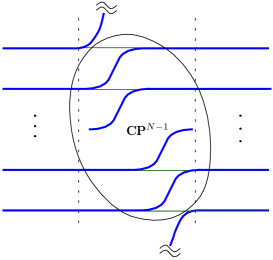
Fig. 15: Brane configuration for one vortex for $N_{\rm F}=N_{\rm C}=N$

We again recover the single vortex moduli space ${\bf C}\times{\bf C}P^{N-1}$ found in [16] in the limit of $\hat{R}\to 0$. Let us note that we cannot take the limit of $\hat{R}\rightarrow\infty$ to obtain meaningful wall configurations in the present case of $N_{\rm C}=N_{\rm F}$, since the larger wall becomes infinitely massive. We need to send the infinitely massive wall to infinity to decouple it, resulting in the unique vacuum without any walls, in conformity with our consideration in (2.17). @

5.3 Double non-Abelian vortices from kinky branes

We now discuss the multi-vortex moduli space by using the kinky D-branes. When $k$ vortices are well separated the moduli space tends to the symmetric product of $k$ single vortex moduli spaces, $({\bf C}\times{\bf C}P^{1})^{k}/\mathfrak{S}_{k}$, with $\mathfrak{S}_{k}$ denoting the permutation group [24]. However the most important thing is how the moduli space looks when two or more vortices collide. This problem was discussed in [23] in the case of $k=2$ for the moduli space proposed in [15], and has been clarified completely in [24] for general $N$ and $k$, by solving the BPS equations. Orbifold singularities of the symmetric product are resolved in the same manner with the Hilbert scheme for the case of instantons, resulting in a smooth moduli manifold. In this section, we discuss this problem by using the kinky D-brane configuration of the T-dual picture.

For simplicity, we restrict ourselves to two vortices ($k=2$) in the $N=2$ case, but we can easily generalize our consideration to arbitrary $k$ and $N$. In this case the kinky D2-branes wind twice around $S^{1}$ in total. Depending on the relative position of two vortices, D-brane configurations are classified into two essentially different configurations as shown in Fig. 16.

(a) well separated vortices	(b) close vortices

Fig. 16: Brane configurations for two vortices. The left-right arrows denote segments of movable region of small kinks.

In Fig. 16 (a) two vortices are well separated compared with the ANO vortex size $1/g\sqrt{c}$ and the configuration is just a sum of two configurations of one vortex in Fig. 11. In Fig. 16 (b) the two vortices are close to each other as their distance is comparable with the vortex size $1/g\sqrt{c}$. The fact that the configuration of close vortices requires a separate treatment is the first sign that the moduli space is not just a symmetric product. It is interesting to note that each D2 brane is configuration of a semi-local vortex in Fig. 10 (b) or its inverse.

We can extract the moduli space of two vortices from these figures. When they are well separated there exist two copies of single vortices: the two large kinks give two ${\bf C}^{*}$ factors while the positions of the two small kinks are bounded from both sides (see Fig. 16-(a)) just as in the single vortex case, giving two ${\bf C}P^{1}$ factors. Therefore as found in [23, 24] asymptotic behavior of the moduli space of well separated vortices is found to be

$$\mathcal{M}_{N_{\rm C}=N_{\rm F}=2}^{k=2}\sim({\bf C}^{*}\times{\bf C}P^{1})^{2}/\mathfrak{S}_{2}.$$ (5.4)

However when the two vortices are close to each other, the situation becomes very different. In this case each small kink cannot move fully inside one large kink unlike well separated vortices because its position is bounded by the identical D-brane on one side, where reconnection does not occur as seen in Fig. 16-(b). Their phases still shrink there resulting in in ${\bf C}P^{1}$’s again but their sizes are smaller than those in the case of the well separated vortices.

Let us discuss how two vortices collide in more detail. All possible configurations for close vortices are drawn in Fig. 17 and are summarized in Table 3.

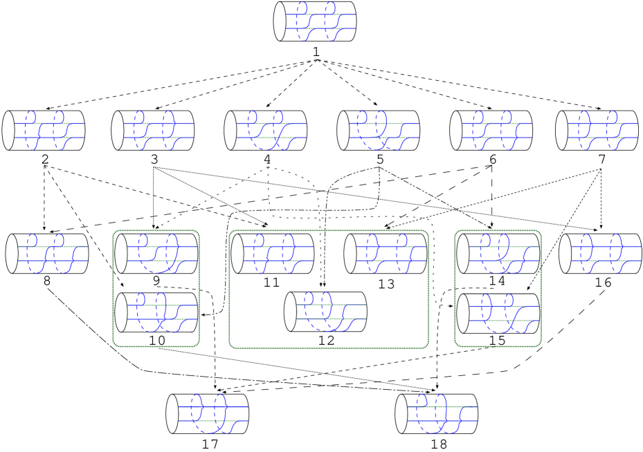
Fig. 17: Brane configuration for two vortices.

Config.	1	2	3	4	5	6	7	8	9	10	11	12	13	14	15	16	17	18
dimC	4	3	3	3	3	3	3	2	2	2	2	2	2	2	2	2	1	1
$I$	0	-1	-1	0	0	1	1	2	-1	-1	0	0	0	1	1	-2	2	-2

Table 3: Moduli subspaces of two vortices.

Each arrow in Fig. 17 denotes a suitable limit of one complex moduli parameter, resulting in a moduli subspace with complex dimension reduced by one. Hence the obtained subspace is a boundary of the space before taking the limit. Generic configuration of two vortices with full moduli dimension (complex dimension four) is shown as the top figure. This configuration has six configurations (with the numbers from 2 to 7 in Fig. 17) on its boundaries, as listed in the second line. They are in complex dimension three and have the intersection number $I$ from $-1$ to $1$. All of them contain one ${\bf C}P^{1}$ factor and their moduli subspaces are like ${\bf C}^{*}\times{\bf C}P^{1}\times{\bf R}^{+}\times S^{1}$. Two vortices lie in the same $U(1)$ subgroup in the configurations 2 and 3 in Fig. 17.

In the third and fourth line the moduli boundaries reduced by one more complex dimension are listed (the configurations with the numbers from 8 to 16). They have the intersection number $I$ from $-2$ to $2$. Interestingly the two (three) configurations with $I=\pm 1$ ($I=0$) bounded by boxes in Fig. 17 are connected to each other without causing reconnection, unlike the configurations in the second line. The three configurations with $I=0$ represent two vortices with different orientations. They can pass through each other without interaction, resulting in the moduli subspace $({\bf C}^{*})^{2}$. More interesting phenomenon can be found in the $I=-1$ case. The movable position of the small kink in $I=-1$ is bounded from both sides like the single vortex case, resulting in a ${\bf C}P^{1}$ factor again. However the size of this ${\bf C}P^{1}$ is twice of that of the single vortex as was found in [23]. In our configuration this phenomenon can be explained as follows. The large kinks denote two coincident ANO vortices. The size of two coincident ANO vortices is $\sqrt{2}$ times that of single ANO vortex, if we assume that energy density is a step function with respect to a radius. This fact implies that the movable region of the small kink is $\sqrt{2}$ times that of the single vortex ($\frac{1}{g\sqrt{c}}$). This is effectively obtained by replacing $g^{2}$ by $g^{2}/2$. Since the Kähler potential for the single vortex moduli is given by $K\sim\frac{1}{g^{2}}\log(1+|b|^{2})$, we have $K\sim\frac{2}{g^{2}}\log(1+|b|^{2})$ for coincident two vortices. Thus the size of orientational modulus in the internal space has been explained by the size of the ANO vortices in the real space. The configurations with $I=+1$ also have a ${\bf C}P^{1}$ factor. In the configuration with $I=\pm 2$ the identical D2-brane winds twice around $S^{1}$ with the rest remains straight. These two vortices lie in the same $U(1)$ subgroup, and the configuration is the same with the case of two ANO vortices, resulting in the moduli space $({\bf C}^{*})^{2}/\mathfrak{S}_{2}$.

In the bottom line two configurations are drawn. Apparently both of them represent two coincident ANO vortices, resulting in the modulus ${\bf C}^{*}$.

To summarize, the moduli subspaces with complex dimension $d$ have been obtained as

$${\mathcal{M}}|^{d=4}\simeq({\bf C}^{*}\times{\bf C}P^{1})^{2}/\mathfrak{S}_{2},$$

$${\mathcal{M}}|^{d=3}_{I=0,\pm 1}\simeq{\bf C}^{*}\times{\bf C}P^{1}\times{\bf R}^{+}\times S^{1},$$

$${\mathcal{M}}|^{d=2}_{I=0}\simeq({\bf C}^{*})^{2},\quad{\mathcal{M}}|^{d=2}_{I=\pm 1}\simeq{\bf C}^{*}\times{\bf C}P^{1},\quad{\mathcal{M}}|^{d=2}_{I=\pm 2}\simeq({\bf C}^{*})^{2}/\mathfrak{S}_{2},$$

$${\mathcal{M}}|^{d=1}_{I=\pm 2}\simeq{\bf C}^{*}.$$ (5.5)

The first one denotes an open set of the symmetric product removing orbifold singularity. By connecting the rest of the moduli subspaces together and placing it to cover the hole of ${\mathcal{M}}|^{d=4}$ we obtain the two vortex moduli space ${\cal M}^{k=2}_{N=2}$. We conclude in this section that kinky configurations (in the large radius limit) give a method alternative to the one in [24] to obtain the smooth full moduli space, but not just the moduli subspace (5.4) for separated vortices.

6 Conclusion and Discussion

We have established the duality between domain walls and vortices. The duality has been investigated from two points of view: field theory and D-brane configurations. In terms of field theory, we have constructed vortices on cylinder $\mathbf{R}\times S^{1}$ as periodically arranged vortices on $\mathbf{C}$. Then we have found that in the case of $N_{\rm C}=1,N_{\rm F}=2$, a pair of wall-like objects appears when the size of the vortex becomes larger than the period of the cylinder as shown in Fig. 3. We have also obtained usual domain walls by introducing a twisted boundary condition and found that a vortex can be decomposed into $N_{\rm F}$ domain walls. We have explained these phenomena as a T-duality between the D-brane configurations of vortices (Fig. 6) and domain walls (Fig. 9). By using this duality, we have found some correspondence between the moduli space of non-Abelian vortices and kinky D-brane configurations for domain walls. The dimensionality of the vortex moduli space can be calculated from its dual kinky brane configuration. The moduli spaces of single and double non-Abelian vortices have been explored in terms of the kinky brane configurations.

Here we give several discussions.

Vortices on a torus

In this paper, we have not considered two T-dualities along directions orthogonal to identical vortices. In order to do that, we have to consider vortices on a torus $T^{2}$ (see, e.g., Ref. [58] for analysis of the ANO vortices on $T^{2}$). This should be useful for construction of vortices if we remember that instantons on $T^{4}$ are related with the ADHM construction of instantons (the Nahm transformation). We expect that a reminiscent of the ADHM construction is obtained for vortices by taking T-dualities twice. This remains as an important future work.

T-duality between $1/4$ BPS composite states

A T-duality between a $1/4$ BPS state of instantons as vortices in the worldvolume of a single vortex in $d=6$ ($d=5$) gauge theory with massless hypermultiplets and $1/4$ BPS state of monopoles as kinks in it in $d=5$ ($d=4$) gauge theory with hypermultiplets with real masses was established previously in [52] through 1/4 BPS calorons in it. This analysis was done in the level of the effective theory, the ${\bf C}P^{N-1}$ model, on the vortex, which is completely parallel to the one in this paper.

On the other hand, domain walls can make a junction or more generally a web (or network) as a $1/4$ BPS state in $d=4$ or $d=3$ gauge theory with complex masses for hypermultiplets [49, 50, 46]. This $d=4$ theory can be obtained by two Scherk-Schwarz dimensional reductions from $d=6$ theory with massless hypermultiplets. Accordingly the domain wall junction carries, at the junction point, the junction charge interpreted as the Hitchin charge, which is obtained by two reductions of the instanton charge. In fact, there exists in $d=6$ instantons accompanied with vortices in two directions, say orthogonal to $z=x^{1}+ix^{3}$ and $w=x^{2}+ix^{4}$ [52]. Taking a T-duality along $x^{4}$ this system becomes a $1/4$ BPS state of monopoles, vortices (on $z$) and domain walls (orthogonal to $x^{2}$) in $d=5$ theory with real masses for hypermultiplets [51]. Taking a T-duality once again along $x^{3}$ the system becomes $1/4$ BPS webs of domain walls in $d=4$ theory with complex masses for hypermultiplets. Thus all $1/4$ BPS states analyzed so far are connected by T-duality maps established in this paper.

Another series of 1/4 BPS equations and the unique set of 1/8 BPS equations have been found in [59, 60]. In particular the set of 1/8 BPS equations is obtained by considering vortices living on all possible two-dimensional planes orthogonal to each other in $d=6$ (in addition to instantons), and all 1/2, 1/4 and 1/8 BPS equations in dimensions less than $d=6$ are obtained by ordinary and/or the SS dimensional reductions [60]. Therefore they must be related through T-duality discussed in this paper. The brane construction of configurations for these newly found equations and T-duality among them remain as a future problem.

Similarity with dyonic instantons as a supertube

Dyonic instantons in $d=5$ gauge theory with sixteen supercharges are instantons with electric flux [61]. They can be interpreted as a supertube [62] as follows [63]. The $d=5$, $U(2)$ gauge theory is realized on the world volume on two D$4$-branes. Dyonic instantons in this theory can be interpreted as a tubular D$2$-brane (a supertube) connected to the two separated D$4$-branes, carrying charges of D$0$-branes and fundamental strings. A ring made of ending points of D$2$-branes on a D$4$-brane is regarded as a loop of a monopole-string, with the total monopole charge being zero. It is known that this ring can be deformed to arbitrary shape by changing moduli [64]. As an extreme case it can be deformed to a set of parallel monopole-sting and anti-monopole-string, where both of them are BPS preserving the same supercharges and therefore the total system is BPS. This situation is completely parallel to our analysis in this paper. Namely, the shape of semi-local vortex can be deformed by changing moduli to a set of parallel domain wall and anti-domain-wall, both of which are BPS. However we cannot deform the shape of the monopole-loop arbitrarily in our case. To overcome this, we should introduce time-dependence and replace lumps and walls by so-called Q-lumps [65] and Q-walls [27], respectively, which carry electric charges. Then we should be able to change the shape of the monopole-loop arbitrarily, and the situation becomes the same with the case of the supertube completely. These new supertubes in the vortex/wall system are “half” of the supertubes as dyonic instantons in the instanton/monopole system. We expect that this half property should be explained by putting NS5-branes in the brane configuration, like the relation between domain walls and monopoles [48].

Similarity with tachyon condensation.

In this paper, we see annihilation phenomenon of the wall and anti-wall pair, which leaves vortex after annihilation. The wall and anti-wall pair does not mean BPS and anti-BPS pair since the identical fraction of supersymmetry in the system is always preserved during the annihilation process. It is, however, reminiscent of the brane and anti-brane pair annihilation in string theory, where lower dimensional BPS branes survives after tachyon condensation. (See for review [67].) The difference between the BPS and non-BPS system in superstring theory exists in the projections on the fermions like the relation between Type II and Type 0 theory, but essential (bosonic) dynamics should be in common with each other. Indeed, recently, it is shown in [68, 69] that the ADHM/Nahm construction of instantons/monopoles has very good interpretation in terms of the tachyon condensation and the formulation can be extended to various dimensions and other solitons. Although we apply the vortex/wall system to only the BPS soliton system in this paper, we expect that our study sheds new lights also on the tachyon condensation of the non-BPS or non-commutative solitons.

Acknowledgements

We would like to thank Kimyeong Lee and other participants of the workshop “Fundamental Problems and Applications of Quantum Field Theory” held at Yukawa Institute of Theoretical Physics in 19–23 December 2005. This work is supported in part by Grant-in-Aid for Scientific Research from the Ministry of Education, Culture, Sports, Science and Technology, Japan No.17540237 (N. S.) and 16028203 for the priority area “origin of mass” (N. S.). The work of M. N. and K. Ohashi (M. E. and Y. I.) is supported by Japan Society for the Promotion of Science under the Post-doctoral (Pre-doctoral) Research Program. K. Ohta is supported in part by Special Postdoctoral Researchers Program at RIKEN.

References

- [1] E. B. Bogomolnyi, Sov. J. Nucl. Phys. 24, 449 (1976) [Yad. Fiz. 24, 861 (1976)]; M. K. Prasad and C. M. Sommerfield, Phys. Rev. Lett. 35, 760 (1975).
- [2] E. Witten and D. I. Olive, Phys. Lett. B 78, 97 (1978).
- [3] M. F. Atiyah, N. J. Hitchin, V. G. Drinfeld and Y. I. Manin, Phys. Lett. A 65, 185 (1978).
- [4] E. Corrigan and P. Goddard, Annals Phys. 154, 253 (1984).
- [5] W. Nahm, Phys. Lett. B 90, 413 (1980).
- [6] W. Nahm, Phys. Lett. B 93, 42 (1980).
- [7] W. Nahm, BONN-HE-83-16 Presented at 12th Colloq. on Group Theoretical Methods in Physics, Trieste, Italy, Sep 5-10, 1983
- [8] H. Schenk, Commun. Math. Phys. 116, 177 (1988).
- [9] P. J. Braam and P. van Baal, Commun. Math. Phys. 122, 267 (1989).
- [10] D. E. Diaconescu, Nucl. Phys. B 503, 220 (1997) [arXiv:hep-th/9608163].
- [11] K. M. Lee and P. Yi, Phys. Rev. D 56, 3711 (1997) [arXiv:hep-th/9702107].
- [12] A. A. Abrikosov, Sov. Phys. JETP 5, 1174 (1957) [Zh. Eksp. Teor. Fiz. 32, 1442 (1957)]; H. B. Nielsen and P. Olesen, Nucl. Phys. B61, 45 (1973).
- [13] C. H. Taubes, Commun. Math. Phys. 72, 277 (1980).
- [14] T. M. Samols, Commun. Math. Phys. 145, 149 (1992); N. S. Manton and J. M. Speight, Commun. Math. Phys. 236, 535 (2003) [arXiv:hep-th/0205307]; H. Y. Chen and N. S. Manton, J. Math. Phys. 46, 052305 (2005) [arXiv:hep-th/0407011]; J. M. Baptista, Commun. Math. Phys. 261, 161 (2006) [arXiv:math.dg/0411517].
- [15] A. Hanany and D. Tong, JHEP 0307, 037 (2003) [arXiv:hep-th/0306150].
- [16] R. Auzzi, S. Bolognesi, J. Evslin, K. Konishi and A. Yung, Nucl. Phys. B 673, 187 (2003) [arXiv:hep-th/0307287].
- [17] A. Hanany and D. Tong, JHEP 0404, 066 (2004) [arXiv:hep-th/0403158].
- [18] M. Eto, M. Nitta and N. Sakai, Nucl. Phys. B 701, 247 (2004) [arXiv:hep-th/0405161].
- [19] V. Markov, A. Marshakov and A. Yung, Nucl. Phys. B 709, 267 (2005) [arXiv:hep-th/0408235].
- [20] A. Gorsky, M. Shifman and A. Yung, Phys. Rev. D 71, 045010 (2005) [arXiv:hep-th/0412082].
- [21] S. Bolognesi, Nucl. Phys. B 719, 67 (2005) [arXiv:hep-th/0412241].
- [22] M. Shifman and A. Yung, arXiv:hep-th/0501211.
- [23] K. Hashimoto and D. Tong, JCAP 0509, 004 (2005) [arXiv:hep-th/0506022].
- [24] M. Eto, Y. Isozumi, M. Nitta, K. Ohashi and N. Sakai, Phys. Rev. Lett. 96, 161601 (2006) [arXiv:hep-th/0511088].
- [25] R. Auzzi, M. Shifman and A. Yung, arXiv:hep-th/0511150.
- [26] L. Krauss and F. Wilczek, Phys. Rev. Lett. 62, 1221 (1989); M. G. Alford, K. Benson, S. R. Coleman, J. March-Russell and F. Wilczek, Phys. Rev. Lett. 64, 1632 (1990) [Erratum-ibid. 65, 668 (1990)]; Nucl. Phys. B 349, 414 (1991); M. G. Alford, K.-M. Lee, J. March-Russell, J. Preskill, Nucl. Phys. B 384, 251 (1992) [arXiv:hep-th/9112038].
- [27] E. R. C. Abraham and P. K. Townsend, Phys. Lett. B 291, 85 (1992); Phys. Lett. B 295, 225 (1992).
- [28] N. D. Lambert and D. Tong, Nucl. Phys. B 569, 606 (2000) [arXiv:hep-th/9907098].
- [29] J. P. Gauntlett, D. Tong and P. K. Townsend, Phys. Rev. D 64, 025010 (2001) [arXiv:hep-th/0012178];
- [30] J. P. Gauntlett, R. Portugues, D. Tong and P. K. Townsend, Phys. Rev. D 63, 085002 (2001) [arXiv:hep-th/0008221].
- [31] D. Tong, Phys. Rev. D 66, 025013 (2002) [arXiv:hep-th/0202012].
- [32] K. S. M. Lee, Phys. Rev. D 67, 045009 (2003) [arXiv:hep-th/0211058].
- [33] D. Tong, JHEP 0304, 031 (2003) [arXiv:hep-th/0303151].
- [34] M. Arai, M. Naganuma, M. Nitta and N. Sakai, Nucl. Phys. B 652, 35 (2003) [arXiv:hep-th/0211103]; in Garden of Quanta - In honor of Hiroshi Ezawa, Eds. by J. Arafune et al. (World Scientific Publishing Co. Pte. Ltd. Singapore, 2003) pp 299-325 [arXiv:hep-th/0302028].
- [35] M. Arai, M. Nitta and N. Sakai, Prog. Theor. Phys. 113, 657 (2005) [arXiv:hep-th/0307274]; Phys. Atom. Nucl. 68, 1634 (2005) [Yad. Fiz. 68, 1698 (2005)] [arXiv:hep-th/0401102].
- [36] M. Arai, E. Ivanov and J. Niederle, Nucl. Phys. B 680, 23 (2004) [arXiv:hep-th/0312037].
- [37] Y. Isozumi, K. Ohashi and N. Sakai, JHEP 0311, 060 (2003) [arXiv:hep-th/0310189]; JHEP 0311, 061 (2003) [arXiv:hep-th/0310130].
- [38] N. Sakai and Y. Yang, arXiv:hep-th/0505136.
- [39] S. Bolognesi, Nucl. Phys. B 730, 127 (2005) [arXiv:hep-th/0507273]; S. Bolognesi and S. B. Gudnason, arXiv:hep-th/0512132.
- [40] M. Shifman and A. Yung, Phys. Rev. D 70, 025013 (2004) [arXiv:hep-th/0312257].
- [41] Y. Isozumi, M. Nitta, K. Ohashi and N. Sakai, Phys. Rev. Lett. 93, 161601 (2004) [arXiv:hep-th/0404198].
- [42] Y. Isozumi, M. Nitta, K. Ohashi and N. Sakai, Phys. Rev. D 70, 125014 (2004) [arXiv:hep-th/0405194].
- [43] M. Eto, Y. Isozumi, M. Nitta, K. Ohashi, K. Ohta, N. Sakai and Y. Tachikawa, Phys. Rev. D 71, 105009 (2005) [arXiv:hep-th/0503033].
- [44] N. Sakai and D. Tong, JHEP 0503, 019 (2005) [arXiv:hep-th/0501207].
- [45] M. Eto, Y. Isozumi, M. Nitta, K. Ohashi, K. Ohta and N. Sakai, Phys. Rev. D 71, 125006 (2005) [arXiv:hep-th/0412024].
- [46] M. Eto, Y. Isozumi, M. Nitta, K. Ohashi, K. Ohta and N. Sakai, AIP Conf. Proc. 805, 354 (2005) [arXiv:hep-th/0509127].
- [47] D. Tong, arXiv:hep-th/0509216; M. Eto, Y. Isozumi, M. Nitta, K. Ohashi and N. Sakai, arXiv:hep-th/0602170.
- [48] A. Hanany and D. Tong, arXiv:hep-th/0507140.
- [49] M. Eto, Y. Isozumi, M. Nitta, K. Ohashi and N. Sakai, Phys. Rev. D 72, 085004 (2005) [arXiv:hep-th/0506135].
- [50] M. Eto, Y. Isozumi, M. Nitta, K. Ohashi and N. Sakai, Phys. Lett. B 632, 384 (2006) [arXiv:hep-th/0508241].
- [51] Y. Isozumi, M. Nitta, K. Ohashi and N. Sakai, Phys. Rev. D 71, 065018 (2005) [arXiv:hep-th/0405129].
- [52] M. Eto, Y. Isozumi, M. Nitta, K. Ohashi and N. Sakai, Phys. Rev. D 72, 025011 (2005) [arXiv:hep-th/0412048].
- [53] Y. Isozumi, M. Nitta, K. Ohashi and N. Sakai, to appear in the proceedings of “NathFest” at PASCOS conference, Northeastern University, Boston, Ma, August 2004 [arXiv:hep-th/0410150]; Proceedings of 12th International Conference on Supersymmetry and Unification of Fundamental Interactions (SUSY 04), Tsukuba, Japan, 17-23 Jun 2004, edited by K. Hagiwara et al. (KEK, 2004) p.1 - p.16 [arXiv:hep-th/0409110]; M. Eto, Y. Isozumi, M. Nitta, K. Ohashi and N. Sakai, AIP Conf. Proc. 805, 266 (2005) [arXiv:hep-th/0508017].
- [54] M. Eto, Y. Isozumi, M. Nitta, K. Ohashi and N. Sakai, “Solitons in the Higgs phase: The moduli matrix approach,” arXiv:hep-th/0602170.
- [55] T. Vachaspati and A. Achucarro, Phys. Rev. D 44, 3067 (1991); Phys. Rept. 327, 347 (2000) [arXiv:hep-ph/9904229].
- [56] R. S. Ward, Phys. Lett. B 158, 424 (1985); I. Stokoe and W. J. Zakrzewski, Z. Phys. C 34, 491 (1987).
- [57] A. Hanany and E. Witten, Nucl. Phys. B 492, 152 (1997) [arXiv:hep-th/9611230].
- [58] A. Gonzalez-Arroyo and A. Ramos, JHEP 0407, 008 (2004) [arXiv:hep-th/0404022].
- [59] K. Lee and H. U. Yee, Phys. Rev. D 72, 065023 (2005) [arXiv:hep-th/0506256].
- [60] M. Eto, Y. Isozumi, M. Nitta and K. Ohashi, arXiv:hep-th/0506257.
- [61] N. D. Lambert and D. Tong, Phys. Lett. B 462, 89 (1999) [arXiv:hep-th/9907014].
- [62] D. Mateos and P. K. Townsend, Phys. Rev. Lett. 87, 011602 (2001) [arXiv:hep-th/0103030].
- [63] D. s. Bak and K. M. Lee, Phys. Lett. B 544, 329 (2002) [arXiv:hep-th/0206185]; S. Kim and K. M. Lee, JHEP 0309, 035 (2003) [arXiv:hep-th/0307048].
- [64] D. Mateos, S. Ng and P. K. Townsend, Phys. Lett. B 538, 366 (2002) [arXiv:hep-th/0204062]; Y. Hyakutake and N. Ohta, Phys. Lett. B 539, 153 (2002) [arXiv:hep-th/0204161]; D. Bak, Y. Hyakutake and N. Ohta, Nucl. Phys. B 696, 251 (2004) [arXiv:hep-th/0404104].
- [65] R. A. Leese, Nucl. Phys. B 366, 283 (1991); E. Abraham, Phys. Lett. B 278, 291 (1992).
- [66] S. Kim, K. M. Lee and H. U. Yee, arXiv:hep-th/0603179.
- [67] J. A. Harvey, arXiv:hep-th/0102076.
- [68] K. Hashimoto and S. Terashima, JHEP 0509, 055 (2005) [arXiv:hep-th/0507078]; arXiv:hep-th/0511297.
- [69] T. Asakawa, S. Matsuura and K. Ohta, “Construction of Instantons via Tahcyon Condensation,” in preparation.