Probabilities in the Bousso-Polchinski multiverse

Abstract

Using the recently introduced method to calculate bubble abundances in an eternally inflating spacetime, we investigate the volume distribution for the cosmological constant $\Lambda$ in the context of the Bousso-Polchinski landscape model. We find that the resulting distribution has a staggered appearance which is in sharp contrast to the heuristically expected flat distribution. Previous successful predictions for the observed value of $\Lambda$ have hinged on the assumption of a flat volume distribution. To reconcile our staggered distribution with observations for $\Lambda$, the BP model would have to produce a huge number of vacua in the anthropic range $\Delta\Lambda_{A}$ of $\Lambda$, so that the distribution could conceivably become smooth after averaging over some suitable scale $\delta\Lambda\ll\Delta\Lambda_{A}$.

I Introduction

The cosmological constant problem is one of the most intriguing mysteries that we now face in theoretical physics. The observed value of the cosmological constant $\Lambda$ is many orders of magnitude smaller than theoretical expectations and is surprisingly close to the present matter density of the universe,

$$\Lambda_{0}\sim\rho_{m0}\sim 10^{-120}.$$ (1)

As of now, the only plausible explanation for these enigmatic facts has been given in terms of the multiverse picture, which assumes that $\Lambda$ is a variable parameter taking different values in different parts of the universe Weinberg87 ; Linde87 ; AV95 ; Efstathiou ; MSW ; GLV ; Bludman ; AV05 . The probability for a randomly picked observer to measure a given value of $\Lambda$ can then be expressed as AV95

$$P_{obs}(\Lambda)\propto P(\Lambda)n_{obs}(\Lambda),$$ (2)

where $P(\Lambda)$ has the meaning of the volume fraction of the regions with a given value of $\Lambda$ and $n_{obs}(\Lambda)$ is the number of observers per unit volume. Disregarding the possible variation of other “constants” and assuming that the density of observers is roughly proportional to the fraction of matter clustered in large galaxies,

$$n_{obs}(\Lambda)\propto f_{G}(\Lambda),$$ (3)

one finds that the function $n_{obs}(\Lambda)$ is narrowly peaked around $\Lambda=0$, with a width

$$\Delta\Lambda_{A}\sim 100\Lambda_{0}\sim 10^{-118}.$$ (4)

In general, the volume factor $P(\Lambda)$ depends on the unknown details of the fundamental theory and on the dynamics of eternal inflation. However, it has been argued AV96 ; Weinberg96 that it should be well approximated by a flat distribution,

$$P(\Lambda)\approx{\rm const}.$$ (5)

The reason is that the anthropic range (4), where the function $n_{obs}(\Lambda)$ is substantially different from zero, is much narrower than the full range of variation of $\Lambda$, which is expected to be set by the Planck scale. A smooth function varying on this large characteristic scale will be nearly constant within the tiny anthropic interval.

Combination of Eqs. (2)-(5) yields the distribution

$$P_{obs}(\Lambda)\propto f_{G}(\Lambda),$$ (6)

which can be readily calculated using the Press-Schechter approximation for $f_{G}$. The observed value of $\Lambda$ is within the $2\sigma$ range of this distribution – an impressive success of the multiverse paradigm. One should keep in mind, however, that the successful prediction for $\Lambda$ hinges on the assumption of a flat volume distribution (5). We emphasize that the form of the volume distribution is important. If, for example, one uses $P(\Lambda)\propto\Lambda$ instead of (5), the $2\sigma$ prediction would be $10<\Lambda/\Lambda_{0}<500$ and the observed value of $\Lambda$ would be ruled out at a 99.9% confidence level Pogosian . The heuristic argument for a flat distribution (5) sounds plausible, but it needs to be verified in specific models.

The simplest model with a variable effective cosmological constant is that of a scalar field $\phi$ with a very slowly varying potential $V(\phi)$ Banks84 ; Linde87 . In such models, $\Lambda$ takes a continuum range of values. It has been verified that the resulting volume distribution for $\Lambda$ is indeed flat for a wide range of potentials Weinberg00 ; GV00 ; GV03 . The main challenge one has to face in this type of model is to justify the exceedingly flat potential which is required to keep the field $\phi$ from rolling downhill on the present Hubble time scale.

A model with a discrete spectrum of $\Lambda$ was first suggested by Abbott Abbott . He considered a scalar field with a “washboard” potential, having many local minima separated by barriers. Transitions between the minima could occur through bubble nucleation. An alternative discrete model, first introduced by Brown and Teitelboim BT , assumes that the cosmological constant can be expressed as

$$\Lambda=\Lambda_{bare}+F^{2}/2.$$ (7)

Here, $\Lambda_{bare}$ is the bare cosmological constant, which is assumed to be large and negative, and $F$ is the magnitude of a four-form field, which can change its value through the nucleation of branes. The change of the field strength across the brane is

$$\Delta F=\pm q,$$ (8)

where the “charge” $q$ is a constant fixed by the model.

In order to explain observations, the discrete spectrum of $\Lambda$ has to be very dense, with separation between adjacent values

$$\Delta\Lambda\lesssim\Lambda_{0},$$ (9)

which in turn requires that the charge $q$ has to be very small. If this is satisfied, analysis shows that the flat volume distribution (5) is quite generic GV01 . But once again, the exceedingly small charge $q$ required by the model appears to be unnatural.

In an effort to remedy this problem, Bousso and Polchinski (hereafter BP) extended the Brown-Teitelboim approach to include multiple four-form fluxes BP . They considered a model in which $J$ different fluxes give rise to a J-dimensional grid of vacua, each labeled by a set of integers $n_{a}$. Each point in the grid corresponds to a vacuum with the flux values $F_{a}=n_{a}q_{a}$ and a cosmological constant

$$\Lambda=\Lambda_{bare}+\frac{1}{2}\sum_{a=1}^{J}F_{a}^{2}=\Lambda_{bare}+\frac{1}{2}\sum_{a=1}^{J}n_{a}^{2}q_{a}^{2}.$$ (10)

This model is particularly interesting because multiple fluxes generally arise in string theory compactifications. The model can thus be regarded as a toy model of the string theory landscape. BP showed that with $J\sim 100$, the spectrum of allowed values of $\Lambda$ can be sufficiently dense, even in the absence of very small parameters, e.g., with $|\Lambda_{bare}|\sim 1$, $q_{a}\sim 0.1$.

In the cosmological context, high-energy vacua of the BP grid will drive exponential inflationary expansion. The flux configuration in the inflating region can change from one point on the grid to the next through bubble nucleation. Bubbles thus nucleate within bubbles, and each time this happens the cosmological constant either increases or decreases by a discrete amount. This mechanism allows the universe to start off with an arbitrary large cosmological constant, and then to diffuse through the BP grid of possible vacua, to generate regions with each and every possible cosmological constant, including that which we inhabit.

Our goal in this paper is to study the volume distribution for $\Lambda$ in the BP model. In particular, we would like to check whether or not this distribution is approximately flat, as suggested by the heuristic argument of AV96 ; Weinberg96 . Until recently, such an analysis would have been rather problematic, since the calculation of the volume fractions in an eternally inflating universe is notoriously ambiguous. The volume of each type of vacuum diverges in the limit $t\to\infty$, so in order to calculate probabilities, one has to impose some kind of a cutoff. The answer, however, turns out to be rather sensitive to the choice of the cutoff procedure. If, for example, the cutoff is imposed on a constant time surface, one gets very different distributions depending on one’s choice of the time variable $t$ LLM . (For more recent discussions, see VVW ; Guth00 ; Tegmark .)

Fortunately, a fully gauge-invariant prescription for calculating probabilities has been recently introduced in GSPVW . It has been tried on some simple models and seems to give reasonable results. Here we shall apply it to the BP model.

As BP themselves recognized, their model does not give an accurate quantitative description of the string theory landscape. In particular, it does not explain how the sizes of compact dimensions get stabilized. This issue was later addressed by Kachru, Kallosh, Linde and Trivedi (KKLT) KKLT , who provided the first example of a metastable string theory vacuum with a positive cosmological constant. Apart from the flux contributions in (10), the vacuum energy in KKLT-type vacua gets contributions from non-perturbative moduli potentials and from branes. The $4D$ Newton’s constant in these vacua depends on the volume of extra dimensions and changes from one vacuum to another. Douglas and collaborators Douglas ; AshokDouglas ; DenefDouglas studied the statistics of KKLT-type vacua. Their aim was to find the number of vacua with given properties (e.g., with a given value of $\Lambda$) in the landscape. Our goal here is more ambitions: we want to find the probability for a given $\Lambda$ to be observed.

In our analysis, we shall disregard all the complications of the KKLT vacua, with the hope that the simple BP model captures some of the essential features of the landscape. At the end of the paper we shall discuss which aspects of our results can be expected to survive in more realistic models.

We begin in the next section by summarizing the prescription of Ref. GSPVW for calculating probabilities. We shall see that the problem reduces to finding the smallest eigenvalue and the corresponding eigenvector of a large matrix, whose matrix elements are proportional to the transition rates between different vacua. The calculation of the transition rates for the BP model is reviewed in Section III. Some of these rates are extremely small, since the upward transitions with an increase of $\Lambda$ are exponentially suppressed relative to the downward transitions. In Section IV we develop a perturbative method for solving our eigenvalue problem, using the upward transition rates as small parameters. This method is applied to the BP model in Section V. We find that the resulting probability distribution has a very irregular, staggered appearance and is very different from the flat distribution (5). The implications of our results for the string theory landscape are discussed in Section VI.

II Prescription for probabilities

Here we summarize the prescription for calculating the volume distribution proposed in Ref. GSPVW . Suppose we have a theory with a discrete set of vacua, labeled by index $j$. The cosmological constants $\Lambda_{j}$ can be positive, negative, or zero. Transitions between the vacua can occur through bubble nucleation. The proposal of Ref. GSPVW is that the volume distribution is given by

$$P_{j}\propto p_{j}Z_{j}^{3},$$ (11)

where $p_{j}$ is the relative abundance of bubbles of type $j$ and $Z_{j}$ is (roughly) the amount of slow-roll inflationary expansion inside the bubble after nucleation (so that $Z_{j}^{3}$ is the volume slow-roll expansion factor).

The total number of nucleated bubbles of any kind in an eternally inflating universe is known to grow without bound, even in a region of finite comoving size. We thus need to cut off our count. The proposal of GSPVW is that the counting should be done at the future boundary of spacetime and should include only bubbles with radii greater than some tiny co-moving size $\epsilon$. The limit $\epsilon\rightarrow 0$ should then be taken at the end. (An equivalent method for calculating $p_{j}$ was suggested in ELM .) It was shown in GSPVW that this prescription is insensitive to the choice of the time coordinate and to coordinate transformations at future infinity.

The bubble abundances $p_{j}$ can be related to the functions $f_{j}(t)$ expressing the fraction of comoving volume occupied by vacuum $j$ at time $t$. These functions obey the evolution equation recycling

$${df_{j}\over{dt}}=\sum_{i}(-\kappa_{ij}f_{j}+\kappa_{ji}f_{i}),$$ (12)

where the first term on the right-hand side accounts for loss of comoving volume due to bubbles of type $i$ nucleating within those of type $j$, and the second term reflects the increase of comoving volume due to nucleation of type-$j$ bubbles within type-$i$ bubbles.

The transition rate $\kappa_{ij}$ is defined as the probability per unit time for an observer who is currently in vacuum $j$ to find herself in vacuum $i$. Its magnitude depends on the choice of the time variable $t$. The most convenient choice for our purposes is to use the logarithm of the scale factor as the time variable; this is the so-called scale-factor time. With this choice,

$$\kappa_{ij}=\Gamma_{ij}{4\pi\over{3}}H_{j}^{-4},$$ (13)

where $\Gamma_{ij}$ is the bubble nucleation rate per unit physical spacetime volume (same as $\lambda_{ij}$ in GSPVW ) and

$$H_{j}=(\Lambda_{j}/3)^{1/2}$$ (14)

is the expansion rate in vacuum $j$.

We distinguish between the recyclable, non-terminal vacua, with $\Lambda_{j}>0$, and the non-recyclable, ”terminal vacua”, for which $\Lambda_{j}\leq 0$. Transitions from either a flat spacetime ($\Lambda_{j}=0$), or a negative $\Lambda$ FRW spacetime ($\Lambda_{j}<0$), which increase $\Lambda$ have a zero probability of occurring. Transitions from $\Lambda_{j}=0$ and from small negative $\Lambda_{j}$ to even more negative $\Lambda$ are possible, but these $\Lambda$’s are likely to be large and negative and are therefore of no anthropic interest. We will label the recyclable, non-terminal vacua by Greek letters, and for non-recyclable, terminal vacua, we will reserve the indices $m$ and $n$. Then, by definition,

$$\Gamma_{\alpha m}=\Gamma_{mn}=0.$$ (15)

Latin letters other than $m,n$ will be used to label arbitrary vacua, both recyclable and terminal, with the exception of letters $a,b$, which we use to label the fluxes.

Eq. (12) can be written in a vector form,

$${d{\bf f}\over{dt}}={\mathbf{M}}{\bf f},$$ (16)

where ${\bf f(t)}\equiv\{f_{j}(t)\}$ and

$$M_{ij}=\kappa_{ij}-\delta_{ij}\sum_{r}\kappa_{ri}.$$ (17)

The asymptotic solution of (16) at large $t$ has the form

$${\bf f}(t)={\bf f^{(0)}}+{\bf s}e^{-qt}+...$$ (18)

Here, ${\bf f}^{(0)}$ is a constant vector which has nonzero components only in terminal vacua,

$$f_{\alpha}^{(0)}=0,$$ (19)

while the values of $f_{n}^{(0)}$ depend on the choice of initial conditions. It is clear from Eq. (15) that any such vector is an eigenvector of the matrix ${\mathbf{M}}$ with zero eigenvalue,

$${\mathbf{M}}{\bf f_{0}}=0.$$ (20)

As shown in GSPVW , all other eigenvalues of $\mathbf{M}$ have a negative real part, so the solution approaches a constant at late times. We have denoted by $-q$ the eigenvalue with the smallest (by magnitude) negative real part and by $\mathbf{s}$ the corresponding eigenvector.

It has been shown in GSPVW that the bubble abundances $p_{j}$ can be expressed in terms of the asymptotic solution (18). The resulting expression is

$$p_{j}\propto\sum_{\alpha}H_{\alpha}^{q}\kappa_{j\alpha}s_{\alpha}.$$ (21)

where the summation is over all recyclable vacua which can directly tunnel to $j$.

Note that the calculation of $p_{j}$ requires only knowledge of the components $s_{\alpha}$ for the recyclable vacua. The evolution of the comoving volume fraction in these vacua is independent of that in the terminal vacua. Formally, this can be seen from the fact that the transition matrix $\mathbf{M}$ in (16) has the form

$$\mathbf{M}=\left(\begin{array}[]{cc}\mathbf{R}&0\\ \mathbf{T}&0\\ \end{array}\right)$$ (22)

Here, $\mathbf{R}$ is a square matrix with matrix elements between recyclable vacua, while the matrix elements of $\mathbf{T}$ correspond to transitions from recyclable vacua to terminal ones. Eigenvectors of $\mathbf{M}$ are of the form ${\bf f}=(\bf s,\bf t)$, where $s$ is an eigenvector of ${\mathbf{R}}$,

$$\mathbf{R}{\bf s}=-q{\bf s},$$ (23)

and ${\bf t}$ is arbitrary. Eigenvalues of $\mathbf{M}$ are the same as those of $\mathbf{R}$, except for some additional zero eigenvalues with eigenvectors which only have nonzero entries for terminal vacua.

The problem of calculating $p_{j}$ has thus been reduced to finding the dominant eigenvalue $q$ and the corresponding eigenvector ${\bf s}$ of the recyclable transition matrix $\mathbf{R}$. In the following sections we shall apply this prescription to the BP model.

III Nucleation rates in the BP model

In the BP model, we have a $J$-dimensional grid of vacua characterized by the fluxes $F_{a}=n_{a}q_{a}$ and vacuum energy densities given by Eq. (10). BP emphasized that $q_{a}$ need not be very small, $q_{a}/|\Lambda_{bare}|\sim 0.1~{}-~{}1$. So the model does not have any small parameters, except perhaps the values of $\Lambda_{j}$ in some vacua, where the contribution of fluxes is nearly balanced by $\Lambda_{bare}$.

Transitions between the neighboring vacua, which change one of the integers $n_{a}$ by $\pm 1$ can occur through bubble nucleation. The bubbles are bounded by thin branes, whose tension $\tau_{a}$ is related to their charge $q_{a}$ as

$$\tau_{a}^{2}=q_{a}^{2}/2.$$ (24)

The latter relation is suggested by string theory BP ; FMSW . It applies only in the supersymmetric limit, but we shall neglect possible corrections due to supersymmetry breaking. Transitions with multiple brane nucleation, in which $|\Delta n_{a}|>1$ or several $n_{a}$ are changed at once, are likely to be strongly suppressed Megevand , and we shall disregard them here.

The bubble nucleation rate $\Gamma_{ij}$ per unit spacetime volume can be expressed as CdL

$$\Gamma_{ij}=A_{ij}\exp^{-B_{ij}}$$ (25)

with

$$B_{ij}=I_{ij}-S_{j}$$ (26)

Here, $I_{ij}$ is the Coleman-DeLuccia instanton action and

$$S_{j}=-{8\pi^{2}\over{H_{j}^{2}}}$$ (27)

is the background Euclidean action of de Sitter space.

In the case of a thin-wall bubble, which is appropriate for our problem, the instanton action $I_{ij}$ has been calculated in Refs. CdL ; BT . It depends on the values of $\Lambda$ inside and outside the bubble and on the brane tension $\tau$.

Let us first consider a bubble which changes the flux $a$ from $n_{a}$ to $n_{a}-1$ ($n_{a}>0$). The resulting change in the cosmological constant is given by

$$|\Delta\Lambda_{a}|=(n_{a}-1/2)q_{a}^{2},$$ (28)

and the exponent in the tunneling rate (25) can be expressed as

$$B_{a\downarrow}=B_{a\downarrow}^{flatspace}r(x,y).$$ (29)

Here, $B_{a\downarrow}^{flatspace}$ is the flat space bounce action,

$$B_{a\downarrow}^{flatspace}=\frac{27\pi^{2}}{2}\frac{\tau_{a}^{4}}{|\Delta\Lambda_{a}|^{3}}.$$ (30)

With the aid of Eqs. (24),(28) it can be expressed as

$$B_{a\downarrow}^{flatspace}=\frac{27\pi^{2}}{8}\frac{1}{(n_{a}-1/2)^{3}q_{a}^{2}}$$ (31)

The gravitational correction factor $r(x,y)$ is given by Parke

$$r(x,y)=\frac{2[(1+xy)-(1+2xy+x^{2})^{\frac{1}{2}}]}{x^{2}(y^{2}-1)(1+2xy+x^{2})^{\frac{1}{2}}}$$ (32)

with the dimensionless parameters

$$x\equiv\frac{3q_{a}^{2}}{8|\Delta\Lambda_{a}|}=\frac{3}{8(n_{a}-1/2)}$$ (33)

and

$$y\equiv\frac{2\Lambda}{|\Delta\Lambda_{a}|}-1,$$ (34)

where $\Lambda$ is the background value prior to nucleation.

The prefactors $A_{ij}$ in (25) can be estimated as

$$A_{ij}\sim 1.$$ (35)

This is an obvious guess for nucleation out of vacua with $\Lambda_{j}\sim 1$. (This guess is supported by the detailed analysis in Ref. Jaume .) For $\Lambda_{j}\ll 1$, we still expect Eq.(35) to hold, since we know that the tunneling rate remains finite in the limit $\Lambda_{j}\to 0$, $|\Delta\Lambda_{a}|\sim 1$.

If the vacuum $n_{a}-1$ still has a positive energy density, then an upward transition from $n_{a}-1$ to $n_{a}$ is also possible. The corresponding transition rate is characterized by the same instanton action and the same prefactor EWeinberg ,

$$I_{ij}=I_{ji},~{}~{}~{}~{}~{}~{}~{}A_{ij}=A_{ji},$$ (36)

and it follows from Eqs.(25), (26) and (14) that the upward and downward nucleation rates are related by

$$\Gamma_{ji}=\Gamma_{ij}\exp\left[24\pi^{2}\left(\frac{1}{\Lambda_{j}}-\frac{1}{\Lambda_{i}}\right)\right].$$ (37)

The exponential factor on the right-hand side of (37) depends very strongly on the value of $\Lambda_{j}$. The closer we are to $\Lambda_{j}=0$, the more suppressed are the upward transitions $j\to i$ relative to the downward ones.

Eq. (37) shows that the transition rate from $n_{a}$ up to $n_{a+1}$ is suppressed relative to that from $n_{a+1}$ down to $n_{a}$. It can also be shown that upward transitions from $n_{a}$ to $n_{a+1}$ are similarly suppressed relative to the downward transitions from $n_{a}$ to $n_{a-1}$. Using Eqs. (28)-(34), the ratio of the corresponding rates can be expressed as

$$\ln(\Gamma_{\downarrow}/\Gamma_{\uparrow})=\Lambda^{-1}f(\Lambda/q_{a}^{2},n_{a}).$$ (38)

The factor $f(\Lambda/q_{a}^{2},n_{a})$ is plotted in Fig. 1 as a function of $\Lambda/q_{a}^{2}$ for $n_{a}=1$ and $n_{a}=2$. The plot shows that upward transitions are strongly suppressed, unless $\Lambda/q_{a}^{2}$ is very large. The factor $\Lambda^{-1}$ in Eq. (38) results in even stronger suppression when $\Lambda$ is well below the Planck scale.

Figure 1: The factor $f(\Lambda/q_{a}^{2},n_{a})$ as a function of $\Lambda/q_{a}^{2}$ for $n_{a}=1$ (solid line), $n_{a}=2$ (dashed line), and $n_{a}=10$ (dotted line).

Transition rates from a given vacuum $j$ to different states $i$ are related by

$$\Gamma_{ij}\propto\exp(-I_{ij}).$$ (39)

As a rule of thumb,

$$I_{ij}\sim-\Lambda_{max}^{-1},$$ (40)

where $\Lambda_{max}$ is the larger of $\Lambda_{i}$ and $\Lambda_{j}$. It follows from (39),(40) that upward transitions from a given site are more probable to the lower-energy vacua.

To develop some intuition for the dependence of the tunneling exponent $B_{a\downarrow}$ on the parameters of the model, we shall consider the limits of small and large $\Lambda$. For $\Lambda\ll|\Delta\Lambda_{a}|$, we have $y\approx-1$, and Eq. (32) gives

$$r(y\to-1)=(1-x)^{-2}>1.$$ (41)

Hence, for low-energy vacua the tunneling exponent is increased over its flat-space value, resulting in a suppression of the nucleation rate. (For small values of $x$, $r$ is increased only by a small fraction, but the factor $B_{a\downarrow}^{flatspace}$ that it multiplies in the tunneling exponent is typically rather large, so the resulting suppression can still be significant.)

In the opposite limit, $\Lambda\gg|\Delta\Lambda_{a}|$, $y\gg 1$,

$$r(y\gg 1)\approx\sqrt{2}(xy)^{-3/2},$$ (42)

and

$$B_{a\downarrow}\approx\frac{27\pi^{2}}{2}q_{a}\left(\frac{2}{3\Lambda}\right)^{3/2}.$$ (43)

The gravitational factor $r$ is plotted in Fig. 2 as a function of $\Lambda/|\Delta\Lambda_{a}|$ for $n_{a}=1$, $n_{a}=2$ and $n_{a}=10$ (corresponding to $x=3/4,~{}1/4$ and $0.04$, respectively). We see that for large values of $\Lambda$, $r\ll 1$, so the nucleation rate is enhanced. In order for our model to be viable, we must ensure that the tunneling action is large enough to justify the use of the semi-classical approximation: $B_{a\downarrow}\gg 1$, or $\Lambda/q_{a}^{2}\ll 20q_{a}^{-4/3}$.

Figure 2: The gravitational factor $r$ as a function of $\Lambda/|\Delta\Lambda_{a}|$ for $n_{a}=1$ (solid line), $n_{a}=2$ (dashed line), and $n_{a}=10$ (dotted line).

If $q_{a}$ and $\Lambda$ are changed simultaneously, keeping the ratios $\Lambda/q_{a}^{2}$ fixed, then $x$ and $y$ do not change, and it is clear from Eqs. (29),(31),(32) that the nucleation exponents scale as $B_{ij}\propto\Lambda^{-1}$. This shows that bubble nucleation rates are strongly suppressed when the energy scales of $q_{a}$ and $\Lambda$ are well below the Planck scale.

IV Perturbation theory

IV.1 Degeneracy factors

We shall assume for simplicity that the integers $n_{a}$ take values in the range $|n_{a}|\leq N$, where $N$ is independent of $a$. The number of vacua in the grid is then $(2N+1)^{J}$.

To maximize computational abilities, we used the symmetry $n_{a}\to-n_{a}$ and restricted the analysis to the sector $0\leq\{n_{a}\}\leq N$. We took into account the degeneracies in $\Lambda$ that would occur if we allowed negative values of $n_{a}$ by assigning appropriate degeneracy factors to the probabilities that we calculated. For example, if we have a two-dimensional grid, $J=2$, and only consider the quadrant $n_{a}\geq 0$, then any point that lies on one of the two axes will be doubly degenerate (configuration $\{0,1\}$ has the same $\Lambda$ as $\{0,-1\}$), whilst a point that lies in the interior of the quadrant will have a four-fold degeneracy (configuration $\{1,2\}$ has the same $\Lambda$ as $\{-1,2\}$, $\{-1,-2\}$, and $\{1,-2\}$).

In general, the degeneracy of each site can be calculated using the following formula:

$${\cal D}\{n_{a}\}=2^{k\{n_{a}\}},$$ (44)

where

$$k\{n_{a}\}=J-(\delta_{0n_{1}}+\delta_{0n_{2}}+...+\delta_{0n_{J}})$$ (45)

So points which have no zero coordinates for a J=7 model have ${\cal D}=2^{7}=128$. A point with one zero coordinate has ${\cal D}=2^{6}=64$ etc.

When we use Eq. (21) to calculate the probabilities, we multiply the RHS by the appropriate degeneracy.

Diffusion from a grid point for which $n=0$ to $n_{a}=-1$, is equivalent to the diffusion from $n=0$ to $n_{a}=+1$. Also, diffusion from $n_{a}=-1$ to $n=0$ is equivalent to $n_{a}=1$ to $n=0$. Thus we were able to take into account these processes in the transition matrix by double counting the positive $n_{a}$ to or from $n=0$ transition rates. In summary, we implemented boundary conditions such that our process is equivalent to diffusion through a J-dimensional grid, with $-N\leq n_{a}\leq N$.

As an illustrative example, we show in Fig. 3 a histogram of the number of vacua vs. $\Lambda$ for a model with $J=7$ and $N=4$, which has $\sim 10^{7}$ vacua. The parameter values used in this model are

$${q_{a}}={0.5308,~{}0.3909,~{}0.5175,~{}0.4722,~{}0.5103,~{}0.4036,~{}0.4541};~{}~{}~{}~{}~{}~{}~{}\Lambda_{bare}=-0.702.$$ (46)

The sharp spikes and dips in the histogram are due partly to the non-uniform distribution of the vacua along the $\Lambda$-axis and partly to the difference in degeneracy factors for different vacua. The spikes disappear when the histogram is plotted with a larger bin size, as shown in Fig.4.

Figure 3: The spectrum of vacua for a $J=7$, $N=4$ BP grid with parameters given in (46).

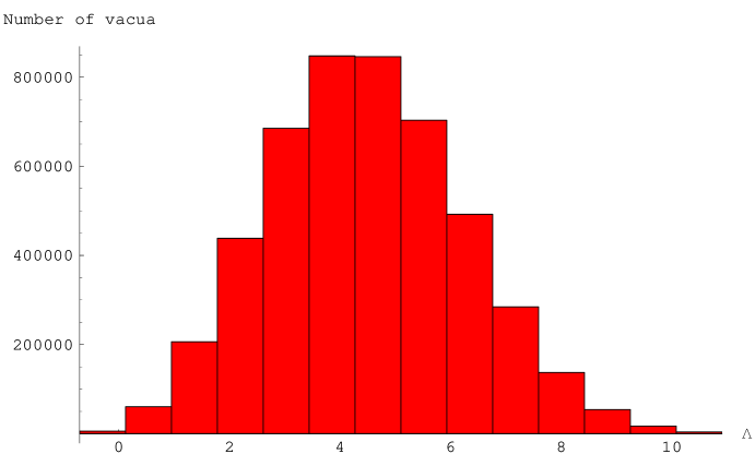
Figure 4: The smoothed spectrum for the above model.

IV.2 Zeroth order

As outlined in Section II, the calculation of probabilities reduces to finding the smallest eigenvalue and the corresponding eigenvector for a huge ${\cal N}\times{\cal N}$ (recycling) transition matrix $\mathbf{R}$. Here, ${\cal N}$ is the number of recyclable vacua, which we expect to be comparable to the total number of vacua. In our numerical example ${\cal N}\sim 10^{7}$, while for a realistic string theory landscape it can be as large as $10^{500}$ Susskind ; Douglas ; AshokDouglas ; DenefDouglas . Matters are further complicated by the fact that some of the elements of $\mathbf{R}$ are exceedingly small. For example, it follows from Eq. (37) that upward transitions from low-energy vacua with $\Lambda_{j}\ll 1$ are very strongly suppressed. Matrix diagonalization programs like Mathematica are not well suited for dealing with such matrices. We shall see, however, that the smallness of the upward transition rates can be used to solve our eigenvalue problem via perturbation theory, with the upward transition rates playing the role of small expansion parameters.

We represent our transition matrix as a sum of an unperturbed matrix and a small correction,

$$\mathbf{R}=\mathbf{R^{(0)}}+\mathbf{R^{(1)}},$$ (47)

where $\mathbf{R^{(0)}}$ contains all the downward transition rates and $\mathbf{R^{(1)}}$ contains all the upward transition rates. We will solve for the zero’th order dominant eigensystem $\{q^{(0)},\mathbf{s^{(0)}}\}$ from $\mathbf{R^{(0)}}$ and then find the first order corrections by including contributions from $\mathbf{R^{(1)}}$. Note that the eigenvalue correction $q^{(1)}$ is not needed for the calculation of bubble abundances (21) to the lowest nonzero order. One only needs to calculate the eigenvector correction $\mathbf{s^{(1)}}$ (since the zeroth-order components $s_{\alpha}^{(0)}$ vanish for recyclable vacua).

If the vacua are arranged in the order of increasing $\Lambda$, so that

$$\Lambda_{1}\leq\Lambda_{2}\leq...\leq\Lambda_{\cal N},$$ (48)

then $\mathbf{R^{(0)}}$ is a triangular matrix, with all matrix elements below the diagonal equal to zero. Its eigenvalues are simply equal to its diagonal elements,

$$R^{(0)}_{\alpha\alpha}=-\sum_{j<\alpha}\kappa_{j\alpha}\equiv-D_{\alpha}.$$ (49)

Hence, the magnitude of the smallest zeroth-order eigenvalue is

$$q^{(0)}=D_{{\alpha_{*}}}\equiv{\rm min}\{D_{\alpha}\}.$$ (50)

Up to the coefficient $(4\pi/3)H_{\alpha}^{-4}$, $D_{\alpha}$ is the total decay rate of vacuum $\alpha$. As we discussed in Section III, bubble nucleation rates are exponentially suppressed in low-energy vacua with $\Lambda_{j}\ll 1$. We therefore expect that the vacuum ${\alpha_{*}}$ corresponding to the smallest eigenvalue $q^{(0)}$ is one of the low-energy vacua.

With $\Lambda_{\alpha_{*}}\ll 1$ and $q_{a}$ not very small, Eq.(28) suggests that downward transitions from ${\alpha_{*}}$ will bring us to the negative-$\Lambda$ territory of terminal vacua. Terminal vacua do not belong in the matrix $\mathbf{R}$; hence, $R_{\beta{\alpha_{*}}}=0$ for $\beta\neq{\alpha_{*}}$, and it is easy to see that our zeroth order eigenvector has a single nonzero component,

$$s^{(0)}_{\alpha}=\delta_{\alpha{\alpha_{*}}}.$$ (51)

Eq. (21) then implies that the only vacua with nonzero probabilities at zeroth order are the negative-$\Lambda$ descendants which can be reached by a single downward jump from the dominant vacuum ${\alpha_{*}}$. (Note that the vacuum $\alpha_{*}$ itself has zero probability at this order.)

IV.3 First order

The full eigenvalue equation can be written as

$$({\mathbf{R}^{(0)}}+{\mathbf{R}^{(1)}})({\bf s^{(0)}}+{\bf s^{(1)}})=-(q^{(0)}+q^{(1)})({\bf s^{(0)}}+{\bf s^{(1)}}).$$ (52)

Neglecting second-order terms and using the zeroth-order relation

$${\mathbf{R}^{(0)}}{\bf s^{(0)}}=-q^{(0)}{\bf s^{(0)}},$$ (53)

we obtain an equation for the first-order corrections,

$$({\mathbf{R}^{(0)}}+q^{(0)}{\mathbf{I}}){\bf s^{(1)}}=-({\mathbf{R}^{(1)}}+q^{(1)}{\mathbf{I}}){\bf s^{(0)}},$$ (54)

where ${\mathbf{I}}$ is the unit matrix.

Eq. (54) is a system of ${\cal N}$ linear equations for the ${\cal N}$ components of ${\bf s^{(1)}}$. Note, however, that the triangular matrix multiplying ${\bf s^{(1)}}$ on the left-hand side has a zero diagonal element,

$$({\mathbf{R}^{(0)}}+q^{(0)}{\mathbf{I}})_{{\alpha_{*}}{\alpha_{*}}}=0,$$ (55)

which means that the determinant of this matrix vanishes, so it cannot be inverted. In other words, the equations in (54) are not all linearly independent.

This problem can be cured by dropping the ${\alpha_{*}}$-th equation in (54) and replacing it by a constraint equation, which we choose to enforce the orthogonality of ${\bf s^{(1)}}$ and ${\bf s^{(0)}}$,

$$({\bf s^{(0)}},{\bf s^{(1)}})=0.$$ (56)

Note that the ${\alpha_{*}}$-th equation is the only equation in (54) that involves the eigenvalue correction $q^{(1)}$. Now $q^{(1)}$ has dropped out of our modified system, and we can straightforwardly solve for $s^{(1)}_{\alpha}$. We did this numerically for a $J=7$ model; the results will be presented in the following subsection. A $J=2$ analytic toy model is worked out in the Appendix.

V Bubble abundances in the BP model

We found in the preceding section that the zeroth order of perturbation theory picks the vacuum $\alpha_{*}$ which decays the slowest (we call it the dominant vacuum), and assigns non-zero probabilities to it’s offspring only - all other probabilities are zero. In the first order of perturbation theory, all vacua connected to the dominant vacuum via one upward jump, and any vacua connected to these via a series of downward transitions, also acquire non-zero probabilities.

The bubble abundance factors $p_{j}$ for the 7-dimensional toy model (46) are shown in Fig. 5. We plot $\log_{10}(1/p_{j})$ vs. $\Lambda_{j}$, so higher points in the figure correspond to smaller bubble abundances. The first thing one notices is that there are several groups of points, marked by triangles, boxes, etc. The star marks the dominant vacuum $\alpha_{*}$.

Figure 5: Plot of $\log_{10}(1/p_{j})$ vs. $\Lambda_{j}$ for the BP model with parameters given in (46). The star marks the dominant vacuum $\alpha_{*}$. Triangles represent vacua in group 1, squares in group 2, diamonds in groups 3 and 6, crosses in groups 4 and 7, and points in groups 5 and 8.

In this particular example, the dominant site has coordinates $(1,1,1,1,1,1,1)$. There are $J=7$ ways to jump up one unit from this site, to arrive at the seven points indicated by black triangles, which we shall call group 1. The coordinates of these points are $(2,1,1,1,1,1,1),~{}(1,2,1,1,1,1,1),~{}...,~{}(1,1,1,1,1,1,2)$. Lower-energy vacua in this group have higher bubble abundances, in accordance with Eqs. (39),(40) of Section III.

The next group of states results from downward jumps out of vacua in group 1 in all possible directions, excluding the jumps back to the dominant site $\alpha_{*}$. We call it group 2. The number of states in this group is $J(J-1)=42$. Consider, for example, the subgroup of states in group 2 coming from the downward transitions out of the state $(2,1,1,1,1,1,1)$. These states have coordinates $(2,0,1,1,1,1,1),~{}...,~{}(2,1,1,1,1,1,0)$. Since they originate from the same single parent, the difference in their bubble abundances comes from the difference in the instanton actions $I_{ij}$. This effect is much milder for downward transitions than it is for the upward ones. That is why the spread in bubble abundances within the subgroups of group 2 is much smaller than it is in group 1.

Further downward jumps replacing one of the $J-2=5$ remaining 1’s by a 0 give rise to group 3, consisting of $J(J-1)(J-2)/{2!}=105$ states having flux configurations with one $n=2$, four $n=1$ and two $n=0$. Similarly, group 4 includes $J(J-1)(J-2)(J-3)/{3!}=140$ states with one $n=2$, three $n=1$ and three $n=0$, and group 5 includes $J(J-1)(J-2)(J-3)(J-4)/4!=105$ states with one $n=2$, two $n=1$ and four $n=0$. The factorial factors are included to avoid double counting. For example, the site $(2,0,1,1,0,1,1)$ can be reached by downward jumps from either $(2,1,1,1,0,1,1)$ or $(2,0,1,1,1,1,1)$ and would be counted twice if we did not divide by $2!$.

If a vacuum in group 2 has a coordinate jump from $n=2$ to $n=1$, the resulting site is one of the daughter sites which can also be reached by downward jumps from the dominant site. These negative-$\Lambda$ vacua have non-zero probabilities already at the zeroth-order level and are not represented in the figure.

If a vacuum in group 3, 4 or 5 has a coordinate jump from $n=2$ to $n=1$, the resulting sites are all terminal vacua (groups 6, 7 and 8, respectively).

We note that although the dominant vacuum $\alpha_{*}$ is one of the low-energy vacua, there are many other recyclable vacua which have lower $\Lambda$. Recall that the dominant vacuum has the smallest, in magnitude, sum of its transition rates down in each possible direction (see Eq.’s (49) and (50)). Each transition rate depends exponentially on the value of $q_{a}$ and the factor $r(x,y)/(n_{a}-1/2)^{3}$. From this factor and Fig.(2) we see that for $\Lambda/\Delta\Lambda<1$ (this is the case for $\alpha_{*}$) any jump from an $n=2$ flux quanta will be less suppressed than a jump in the same direction from an $n=1$ flux quanta. Thus we are not surprised that states which contain a flux quanta of $n=2$ are not dominant sites despite having smaller $\Lambda$ than $\alpha_{*}$. Since each transition rate is exponentially dependent on the tunneling exponent, typically the largest (in magnitude) transition rate will dominate the sum in Eq.(49). Thus, essentially for a vacuum to be the dominant state its largest (in magnitude) transition rate should be smaller that the largest transition rate of any other vacuum.

The distribution in Fig. 5 was obtained in the first order of perturbation theory, which includes only the vacua which can be reached by a single upward jump from the dominant site $\alpha_{*}$, followed by some downward jumps. If higher orders were included, we would see additional groups of vacua, reachable only with two or more upward jumps. These vacua would have much smaller bubble abundances than those already in the figure.

The distribution $p_{j}$ in Fig. 5 spans more than 300 orders of magnitude. It differs dramatically from the flat distribution (5) suggested by the heuristic argument in the Introduction. Many vacua with close values of $\Lambda_{j}$ have very different abundances $p_{j}$. The reason is that despite their closeness in $\Lambda$, such vacua are located far away from one another in the BP grid, and the paths leading to them from the dominant vacuum $\alpha_{*}$ are characterized by exponentially different transition rates. Even the vacua resulting from tunneling out of the same site typically have very different abundances, due to the exponential dependence of the tunneling rates on $q_{a}$.

Fig. 6 shows the distribution of bubble abundances for another $J=7$ model, with a different set of parameters:

$${q_{i}}={0.6175,~{}0.3909,~{}0.6472,~{}0.5508,~{}0.5103,~{}0.7036,0.4541};~{}~{}~{}~{}~{}~{}~{}\Lambda_{bare}=-1.033.$$ (57)

In this case, there is more scatter in the values of $q_{a}$, and the groups of vacua are somewhat less pronounced. However, the staggered nature of the distribution is still apparent.

Figure 6: Plot of $\log_{10}(1/p_{j})$ vs. $\Lambda_{j}$ for the BP model with parameters (57). The star marks the dominant vacuum $\alpha_{*}$. Different groups of vacua are represented by the same symbols as in Fig.5.

VI Discussion

In this paper we have used the prescription of Refs. GSPVW ; ELM to determine the bubble abundances $p_{j}$ in the BP model. We found that the resulting distribution is very irregular, with values of $p_{j}$ soaring and plummeting wildly as $\Lambda_{j}$ changes from one value to the next. This distribution is drastically different from the flat distribution (5) which was used as a basis for the successful anthropic prediction for $\Lambda$.

Apart from the bubble abundance factor $p_{j}$, the volume distribution (11) includes the slow-roll expansion factor $Z_{j}$. In any realistic model, bubble nucleation should be followed by a period of slow-roll inflation, at least in some bubble types. The expansion factor $Z_{j}$ is, of course, model-dependent, but there is no reason to expect that it will somehow compensate for the wild swings in the values of $p_{j}$ as we go from one value of $\Lambda_{j}$ to the next.

Another point to keep in mind is that, in a realistic setting, vacua with different values of the fluxes $F_{a}$ may have different low-energy physics, so the density of observers $n_{obs}(\Lambda)$ would also be very different. We should therefore focus on the subset of vacua in the BP grid which differ only by the value of $\Lambda$ and have essentially identical low-energy constants. Once again, there seems to be no reason to expect any correlation between these constants and the up and down swings in the bubble abundances. We conclude that the staggered character of the distribution $P_{j}\equiv P(\Lambda_{j})$ is expected to persist, even in more realistic versions of the model.

This conclusion is not limited to the BP model. It is likely to arise in any landscape scenario, where a dense spectrum of low-energy constants is generated from a wide distribution of states in the parameter space of the fundamental theory. Vacua with nearly identical values of $\Lambda$ may then come from widely separated parts of the landscape and may have very different bubble abundances and volume fractions.

Given the staggered character of the volume distribution, what kind of prediction can we expect for the observed value of $\Lambda$? The answer depends on the number ${\cal N}_{A}$ of possible vacua with $\Lambda_{j}$ within the anthropic range (4), $\Delta\Lambda_{A}\sim 10^{-118}$. (We count only vacua in which all low-energy constants other than $\Lambda$ have nearly the same values as in our vacuum.)

Suppose the volume factors in the distribution $P_{j}$ span $K$ orders of magnitude. ($K\sim 300$ in our numerical example in Section V.) We can divide all vacua into, say, $10K$ bins, such that the values of $P_{j}$ in each bin differ by no more than $10\%$. Suppose now that there are ${\cal N}_{A}\ll 10K$ vacua in the anthropic range $\Delta\Lambda_{A}$. We can then expect that most of these vacua will be characterized by vastly different volume factors $P_{j}$, so that the entire range will be dominated by one or few values of $\Lambda_{j}$ having much higher volume fractions than the rest.

Moreover, there is a high likelihood of finding still greater volume fractions if we go somewhat beyond the anthropic range - simply because we would then search in a wider interval of $\Lambda$. We could, for example, find that a vacuum with $\Lambda_{1}\sim 10^{-114}\sim 10^{6}\Lambda_{0}$ has a volume fraction 200 orders of magnitude greater than all other vacua in the range $0<\Lambda\lesssim\Lambda_{1}$. Galaxy formation is strongly suppressed in this vacuum: the fraction of matter that ends up in galaxies is only $f_{G}(\Lambda_{1})\sim 10^{-110}$. However, this suppression is more than compensated for by the enhancement in the volume fraction.

If this were the typical situation, most observers would find themselves in rare, isolated galaxies, surrounded by nearly empty space, all the way to the horizon. This is clearly not what we observe. The dominant value could by chance be very close to $\Lambda=0$, but if such an “accident” is required to explain the data, the anthropic model loses much of its appeal.

In the opposite limit, ${\cal N}_{A}\gg 10K$, the number of vacua in the anthropic interval $\Delta\Lambda_{A}$ is so large that they may scan the entire range of $P_{j}$ many times. Then, it is conceivable that the distribution will become smooth after averaging over some suitable scale $\delta\Lambda$. If $\delta\Lambda$ can be chosen much smaller than $\Delta\Lambda_{A}$, then it is possible that the effective, averaged distribution will be flat, as suggested by the heuristic argument in the Introduction. The successful prediction for $\Lambda$ would then be unaffected.

The above argument is somewhat simplistic, as it assumes that the vacua in the BP grid are more or less randomly distributed between the $10K$ bins, with roughly the same number of vacua in each bin. Such an “equipartition” is not likely to apply to the most abundant vacua, but it may hold for the vacua in the mid-range of $P_{j}$. Finding the conditions under which equipartition applies would require a statistical analysis that goes beyond the scope of the present paper.

In summary, it appears that the staggered volume distribution resulting from the BP model is in conflict with observations, unless it yields a huge number of vacua in the anthropic range of $\Lambda$. Counting only vacua which have nearly the same low-energy physics as ours, we should have much more than $10K$; hence, the total number of vacua should be many orders of magnitude greater. The large number of vacua in the anthropic range is only a necessary condition for the distribution $P_{j}$ to average out to the flat distribution (5). Further analysis will be needed to find whether or not this actually happens, and if so, then under what conditions. It would also be interesting to analyze other simple models of the landscape, such as the “predictive landscape” of Arkani-Hamed, Dimopoulos and Kachru AHDK , and see what similarities and differences they have compared to the BP model.

Throughout this paper we assumed that the brane charges $q_{a}$ are not particularly small. This assumption may be violated in certain parts of the landscape, e.g., in the vicinity of conifold points, resulting in a much denser spectrum of vacua FMSW ; AshokDouglas ; DenefDouglas ; Giryavets . Infinite accumulations of vacua may occur near certain attractor points DVattractor ; Gia . Implications of these effects for the probability distribution on the landscape remain to be explored.

VII Acknowledgements

We are grateful to Michael Douglas, Gia Dvali, Jaume Garriga, Ken Olum and Joseph Polchinski for useful comments and discussions. This work was supported in part by the National Science Foundation.

VIII Appendix

We will illustrate our perturbative method of calculation on a very basic BP model, which can be solved analytically. We consider $9$ vacua arranged in a 2-D grid and labeled as indicated in Fig. 7. There are three terminal vacua labeled 1, 2, 4, and six non-terminal vacua, 3, 5, 6, 7, 8, 9 in this model. We allow upward and downward transitions between nearest neighbor pairs, with transitions from non-terminal to terminal states allowed, but no transitions may take place from a terminal state. For simplicity, we disregard the vacua in the quadrants where $n_{1}<0$ and/or $n_{2}<0$ and assume that the set of vacua in Fig.(7) is all there is.

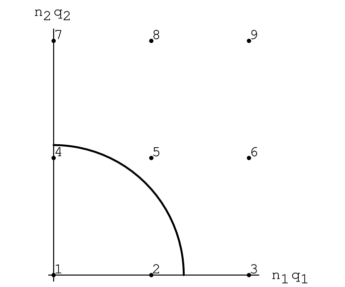
Figure 7: The arrangement of vacua for a $J=2$, $N=2$ BP grid

The evolution equations for the set of non-terminal vacua is

$$\frac{d\mathbf{f}}{dt}=\mathbf{R}\mathbf{f},$$ (58)

where the vector $\mathbf{f}\equiv\{f_{3},f_{5},f_{6},f_{7},f_{8},f_{9}\}$. Assuming that upward transition rates are far more suppressed than downward transition rates, we represent the transition matrix as

$$\mathbf{R}=\mathbf{R^{(0)}}+\mathbf{R^{(1)}},$$ (59)

where

$$\mathbf{R^{(0)}}=\left(\begin{array}[]{cccccc}-D_{3}&0&\kappa_{36}&0&0&0\\ 0&-D_{5}&\kappa_{56}&0&\kappa_{58}&0\\ 0&0&-D_{6}&0&0&\kappa_{69}\\ 0&0&0&-D_{7}&\kappa_{78}&0\\ 0&0&0&0&-D_{8}&\kappa_{89}\\ 0&0&0&0&0&-D_{9}\\ \end{array}\right)$$ (60)

and

$$\mathbf{R^{(1)}}=\left(\begin{array}[]{cccccc}-U_{3}&0&0&0&0&0\\ 0&-U_{5}&0&0&0&0\\ \kappa_{63}&\kappa_{65}&-U_{6}&0&0&0\\ 0&0&0&-U_{7}&0&0\\ 0&\kappa_{85}&0&\kappa_{87}&-U_{8}&0\\ 0&0&\kappa_{96}&0&\kappa_{98}&-U_{9}\\ \end{array}\right)$$ (61)

and we have defined

$$D_{\alpha}\equiv\sum_{j<\alpha}\kappa_{j\alpha},$$ (62)

$$U_{\alpha}\equiv\sum_{j>\alpha}\kappa_{j\alpha}.$$ (63)

$D_{\alpha}$ and $U_{\alpha}$ represent, respectively, the sum of the downward and upward transition rates from vacuum $\alpha$.

In our toy model we will assume that vacuum $5$ has the smallest (in magnitude) sum of downward transition rates, and therefore $-q^{(0)}=-D_{5}$ is the zero’th order dominant eigenvalue. By inspection, we see that the corresponding eigenvector is $\mathbf{s^{(0)}}\equiv\{0,1,0,0,0,0\}$.

We now need to calculate the first order correction to this eigenvector, $\mathbf{s^{(1)}}$. Substituting (60),(61) in Eq. (54), we find

$$\left(\begin{array}[]{cccccc}q^{(0)}-D_{3}&0&\kappa_{36}&0&0&0\\ 0&0&\kappa_{56}&0&\kappa_{58}&0\\ 0&0&q^{(0)}-D_{6}&0&0&\kappa_{69}\\ 0&0&0&q^{(0)}-D_{7}&\kappa_{78}&0\\ 0&0&0&0&q^{(0)}-D_{8}&\kappa_{89}\\ 0&0&0&0&0&q^{(0)}-D_{9}\\ \end{array}\right)\mathbf{s^{(1)}}=\left(\begin{array}[]{c}0\\ -q^{(1)}+U_{5}\\ -\kappa_{65}\\ 0\\ -\kappa_{85}\\ 0\\ \end{array}\right)$$ (64)

Note that the only equation in this set that depends on the first order correction to the eigenvalue is also the equation that needs to be dropped from our system, since it has a zero diagonal element - this causes the matrix on the right-hand side of (64) to have a zero determinant, which renders it uninvertible.

This drop in the number of independent equations is replenished by including the constraint equation (56); the resulting set of equations is

$$\left(\begin{array}[]{cccccc}q^{(0)}-D_{3}&0&\kappa_{36}&0&0&0\\ 0&1&0&0&0&0\\ 0&0&q^{(0)}-D_{6}&0&0&\kappa_{69}\\ 0&0&0&q^{(0)}-D_{7}&\kappa_{78}&0\\ 0&0&0&0&q^{(0)}-D_{8}&\kappa_{89}\\ 0&0&0&0&0&q^{(0)}-D_{9}\\ \end{array}\right)\mathbf{s^{(1)}}=\left(\begin{array}[]{c}0\\ 0\\ -\kappa_{65}\\ 0\\ -\kappa_{85}\\ 0\\ \end{array}\right)$$ (65)

The solution is readily determined, and we obtain

$$\mathbf{s^{(1)}}=\left(\begin{array}[]{c}\frac{\kappa_{36}}{D_{3}-D_{5}}\frac{\kappa_{65}}{D_{6}-D_{5}}\\ 0\\ \frac{\kappa_{65}}{D_{6}-D_{5}}\\ \frac{\kappa_{78}}{D_{7}-D_{5}}\frac{\kappa_{85}}{D_{8}-D_{5}}\\ \frac{\kappa_{85}}{D_{8}-D_{5}}\\ 0\\ \end{array}\right)$$ (66)

This can now be used in Eq.(21) to determine the bubble abundances. For example, comparing the bubble abundances in vacua 3 and 7, we find

$$\frac{p_{3}}{p_{7}}={H_{6}^{q}\kappa_{36}\kappa_{65}(D_{8}-D_{5})\over{H_{8}^{q}\kappa_{78}\kappa_{85}(D_{6}-D_{5})}}$$ (67)

References

- (1) S. Weinberg, Phys. Rev. Lett. 59, 2607 (1987).
- (2) A.D. Linde, in 300 Years of Gravitation, ed. by S.W. Hawking and W. Israel, (Cambridge University Press, Cambridge, 1987).
- (3) A. Vilenkin, Phys. Rev. Lett. 74, 846 (1995).
- (4) G. Efstathiou, M.N.R.A.S. 274, L73 (1995).
- (5) H. Martel, P. R. Shapiro and S. Weinberg, Ap.J. 492, 29 (1998).
- (6) J. Garriga, M. Livio and A. Vilenkin, Phys. Rev. D61, 023503 (2000).
- (7) S. Bludman, Nucl. Phys. A663-664,865 (2000).
- (8) For a review, see, e.g., A. Vilenkin, “Anthropic predictions: the case of the cosmological constant”, astro-ph/0407586.
- (9) A. Vilenkin, in Cosmological Constant and the Evolution of the Universe, ed by K. Sato, T. Suginohara and N. Sugiyama (Universal Academy Press, Tokyo, 1996).
- (10) S. Weinberg, in Critical Dialogues in Cosmology, ed. by N. G. Turok (World Scientific, Singapore, 1997).
- (11) L. Pogosian, private communication.
- (12) T. Banks, Phys. Rev. Lett. 52, 1461 (1984).
- (13) S. Weinberg, Phys. Rev. D61 103505 (2000); astro-ph/0005265.
- (14) J. Garriga and A. Vilenkin, Phys. Rev. D61, 083502 (2000).
- (15) J. Garriga and A. Vilenkin, Phys. Rev. D67, 043503 (2003) (corrected version at astro-ph/0210358).
- (16) L. F. Abbott, Phys. Lett. B150, 427 (1985).
- (17) J. D. Brown and C. Teitelboim, Phys. Lett. B195, 177 (1987); Nucl. Phys. B297, 787 (1988).
- (18) J. Garriga and A. Vilenkin, Phys. Rev. D64, 023517 (2001).
- (19) J. Donoghue, JHEP 0008:022 (2000).
- (20) J.L. Feng, J. March-Russell, S. Sethi and F. Wilczek, Nucl. Phys. B602, 307 (2001).
- (21) T. Banks, M. Dine and L. Motl, JHEP 0101, 031 (2001).
- (22) G. Dvali and A. Vilenkin, Phys. Rev. D64, 063509 (2001).
- (23) R. Bousso and J. Polchinski, JHEP 0006, 006 (2000).
- (24) A. D. Linde, D. A. Linde, and A. Mezhlumian, Phys. Rev. D 49, 1783 (1994).
- (25) V. Vanchurin, A. Vilenkin, and S. Winitzki, Phys. Rev. D 61, 083507 (2000).
- (26) A. H. Guth, Phys. Rept. 333, 555 (2000).
- (27) M. Tegmark, JCAP 0504, 001 (2005).
- (28) J. Garriga, D. Schwartz-Perlov, A. Vilenkin and S. Winitzki, “Probabilities in the inflationary multiverse”, hep-th/0509184.
- (29) S. Kachru, R. Kallosh, A. Linde and S. Trivedi, Phys. Rev. D68, 046005 (2003).
- (30) M.R. Douglas, JHEP 0305, 046 (2003).
- (31) S. Ashok and M.R. Douglas, JHEP 0401, 060 (2004).
- (32) F. Denef and M.R. Douglas, JHEP 0405, 072 (2004).
- (33) R. Easther, E.A. Lim and M.R. Martin, “Counting pockets with world lines in eternal inflation”, arXiv:astro-ph/0511233.
- (34) J. Garriga and A. Vilenkin, Phys. Rev. D57, 2230 (1998).
- (35) J. Garriga and A. Megevand, Phys. Rev. D69, 083510 (2004).
- (36) S. Coleman and F. DeLuccia, Phys. Rev. D21, 3305 (1980).
- (37) S. Parke, “Gravity and the decay of the false vacuum”, Phys. Letters B 121 (1983) 313.
- (38) J. Garriga, Phys. Rev. D 49 (1994) 6327.
- (39) K. M. Lee and E. J. Weinberg, Phys. Rev. D 36, 1088 (1987).
- (40) L. Susskind, “The anthropic landscape of string theory,” arXiv:hep-th/0302219.
- (41) A. Giryavets, S. Kachru and P.K. Tripathy, JHEP 0408, 002 (2004).
- (42) G. Dvali and A. Vilenkin, Phys. Rev. D70, 063501 (2004).
- (43) G. Dvali, “Large hierarchies from attractor vacua”, arXiv:hep-th/0410286.
- (44) N. Arkani-Hamed, S. Dimopoulos and S. Kachru, “Predictive landscapes and new physics at a TeV”, arXiv:hep-th/0501082.