IFUM-859-FT

January 2006

$\mathcal{M}echanisms\ for\ Supersymmetry$

$\mathcal{\ }Breaking\ in\ Open\ String\ Vacua$

 

Matteo A. Cardella

Dipartimento di Fisica dell’Università di Milano and

INFN, Sezione di Milano, Via Celoria 16, 20133 Milano, Italy

Abstract

We investigate mechanisms that can trigger supersymmetry breaking in open string vacua. The focus is on backgrounds with D-branes and orientifold planes that have an exact string description, and allow to study some of the quantum effects induced by supersymmetry breaking.

 

e-mail: matteo.cardella@mi.infn.it

——————————————————————————————————————-

Università degli Studi di Milano

Facoltà di Scienze Matematiche, Fisiche e Naturali

Corso di Dottorato in Fisica, Astrofisica e Fisica Applicata

XVIII ciclo

Tesi di Dottorato di Ricerca

$\mathcal{M}echanisms\ for\ Supersymmetry\ Breaking$

$\mathcal{\ }in\ Open\ String\ Vacua$

(settore scientifico disciplinare: FIS/02)

Candidato:

Matteo Aureliano Cardella

matr. R05128

Relatore Interno:

Prof. Daniela Zanon

Relatore Esterno:

Dr. Carlo Angelantonj

Coordinatore:

Prof. Gianpaolo Bellini

Anno Accademico 2004-2005

————————————————————————————————————–

————————————————————————————————————–

Chapter 1 Introduction

String Theory is a quite interesting framework with the promising characteristics to provide a unified scheme that incorporates the fundamental interactions. One of its ambitious goals is to describe the status of space-time and matter in the early instants after the Big Bang.

In its perturbative formulation String Theory replaces the concept of point particles with one-dimensional objects, whose internal quantum vibrational modes gives rise to a certain number of massless states plus an infinite tower of massive ones. The main result is to identify the different particles of the Standard Model together with the graviton as different quantum states of a single entity. Indeed this replacement solves the UV-divergence problems that plague any attempt of constructing a consistent quantum field theory for a spin-two particle (the graviton) on Minkowski space-time .

The Action for a string propagating on a given space-time has the peculiar feature of being classically invariant under local rescaling of the world-sheet metric (2d-conformal transformations). The request for this symmetry to survive after quantisation puts strong constraints on the number $D$ of space-time dimensions, on the equations for the background fields and on the spectrum of string vibrations. In the critical dimension $D_{crit}$ the world-sheet scale factor decouples from the dynamics after quantisation, while for a different number of dimensions the quantum (conformal) theory acquires an extra-dimension given by the coupled scale factor mode. For the fermionic string $D_{crit}=10$, and the only stable solutions on a ten-dimensional Minkowski space-time enjoy supersymmetry, which therefore represents an important ingredient in all the constructions. For supersymmetric string theories the equation of motions for the background fields at leading order in the string length agree with Einstein equations in the vacuum, and consistently one of the massless states of the closed string can be identified with the graviton.

There are five ten-dimensional perturbative string theories: type IIA, type IIB, type I and the two Heterotic ones, that, together with eleven-dimensional supergravity, are interconnected via a rich web of dualities, relating their various weak and strong coupling regimes.

This has led to the conclusion that these are indeed different perturbative corners of a unique conjectured theory called M-theory, whose fundamental degrees of freedom and formulation remain so far unknown.

A fundamental role in order to establish these dualities and, to gain some insights in the non-perturbative regime of the theory, has been played by the Dirichlet p-branes, extended objects that are sources for multidimensional generalisations of the Maxwell potential called the Ramond-Ramond forms. Dirichlet p-branes are regarded as solitons of the theory, carrying a charge and a tension proportional to the inverse of the string coupling constant, and quite remarkably having open strings as their quantum excitations.

It is fascinating to look at these extended objects as space-time defects (figure 1.1), remnants of a phase transition that might have occurred during the cooling down of the universe after the Big Bang. It is remarkable as well how the mathematical consistency of string theory suggests their existence, by including the multidimensional generalisation of Maxwell potentials (Ramond-Ramond fluxes) in one sector of its perturbative closed-string spectra.

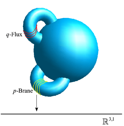
Figure 1.1: An image of the possible structure of space-time after a phase transition from an unknown quantum gravity regime: six of the original dimensions are compact (in the figure only two of them are represented), while four are extended, (represented by the straight line). Flux lines are trapped in the topology of the compact space, while p-branes are space-time defects that can wrap some of the non-contractible circles and invade the extended dimensions.

The flat ten-dimensional solutions are regarded as a guide to produce a much larger class of new solutions, via a process of symmetry breaking called compactification. Among them, of particular interest are those where six of the ten dimensions are highly curled up to form a compact space, and the full space-time factorises as the product of the four-dimensional Minkowski space times this compact space. All these solutions are considered as different vacua of the same theory and, due to the present lack of a non-perturbative formulation, it is not possible to fully understand the relations among these different vacua. Therefore it is quite hard to address the question of whether the theory prefers a vacuum rather than another, an open issue that goes under the name of vacuum degeneracy problem.

The perturbative nature of the world-sheet formulation results from an initial splitting of the space-time metric in a classical background plus quantum stringy fluctuations. This approach does not address the problem of finding the symmetries and principles that need to replace General Covariance, in order to obtain a fully consistent fusion between Quantum Mechanics and General Relativity.

In a classical spin-two field theory on Minkowsky space-time, if one starts by considering only a three-points self-interaction, in order to achieve a ghost-free field theory one needs to add higher and higher interaction vertexes to the Lagrangian. The final result is a non-polynomial action, from which, without the knowledge of the underlying geometrical principles, it would be quite hard to recognise General Covariance behind its nice properties.

A similar state of affairs happens in string theory, with the advantage, with respect to the field counterpart, of solving the UV-divergences problem but with the big drawback of not possessing yet enough clues about the new geometrical ideas. The description of quantum gravity as string fluctuation on a non-dynamical space-time is intrinsically perturbative and not manifestly background independent. The non-perturbative formulation is likely to be found through new geometrical principles, counterpart of classical General Covariance, a task that so far has been proved quite hard.

Waiting for new insights toward a non-perturbative formulation, one can still investigate possible mechanisms by working in particular vacua of the theory. There are currently several tasks that are object of intense research in following this last approach, among them of particular relevance is the question of finding a controlled description for the process of moduli stabilisation and (super)symmetry breaking.

If string theory is on the right track it should contain the answers to these questions, and vacua with identical features of the Standard Model. In principle, the Standard Model parameters could be reproduced as the result of moduli stabilisation. Moduli is the name that indicates VEVs of background scalar fields, arising from compactification, some of that describing properties of the compact space.

The second vital question deals with finding mechanisms that break the original supersymmetries, in order to make contact with the Standard Model of particle physics and with the observed value of the Cosmological Constant. Although a complete answer might be found, if ever, from a non-perturbative point of view, still there are several features that can be observed by studying string fluctuations around backgrounds containing non-perturbative objects such as Dirichlet branes and orientifold planes.

Historically the first attempts at looking for semi-realistic vacua have been pursued from compactifications of the Heterotic string. In this case, in order to be in a perturbative regime, both the string scale and the compactification scale need to be not far from the Planck scale. The study of the string dynamics for this class of compactifications is confined to the massless modes and involves the construction of an effective Action. This is obtained by integrating out all the heavy modes, given by string excitations and Kaluza-Klein states, and its form is then determined by supersymmetry and topological data of the compact manifold.

A different approach for looking at semi-realistic vacua that offers a more stringy description was born after a development in the understanding of the role of Dp-branes. For example, in open string vacua in the presence of some large extra-dimensions, the string scale can be lowered to the TeV range in a perturbative description. In this case, massive string excitations do participate to the low-energy dynamics, so that their effects can be taken into account in all the compactifications that allow an exact conformal description. In models of brane-worlds D-p branes invade four extended dimensions, as represented in fig. 1.1, and wrap some cycles of the compact space. The standard model forces are then mediated by open strings confined on the brane, while only gravity, mediated by closed strings, can experience all the ten-spacetime dimensions. This has offered a new explanation for the observed hierarchy between the electro-weak and the gravitational forces. Gravity is so weak because of the dispersion of its flux lines in a higher number of dimensions comparing to the other forces.

In summary, the presence of D-branes opens up the study of new classes of string compactifications, where important open issues such as moduli stabilisation, breaking of supersymmetry, and the hierarchy problem can be studied from a more stringy perspective.

This thesis follows this line of thought for investigating possible mechanisms that can trigger supersymmetry breaking in open string vacua. The focus is on backgrounds with D-branes and orientifold planes that have an exact string descriptions, which allow to study some of the quantum effects of supersymmetry breaking.

In the first chapter I review some of the fundamentals of perturbative string theory, with a final emphasis on one-loop closed string amplitudes and on the informations that the torus amplitude contains about the ten-dimensional closed superstring spectra.

The second chapter describes open string excitations from D-p branes and the introduction of orientifold planes, often necessary to find consistent string backgrounds. The emphasis is on the genus-one open and closed string diagrams that describe type I superstring vacua.

The third chapter deals with supersymmetric toroidal compactifications in the presence of D-branes and orientifold planes and the description of several interesting effects associated to different points in the background moduli space.

Chapter four introduces possible mechanisms for supersymmetry breaking that originate from various configurations of D-branes and O-planes, and among them, a novel mechanism for supersymmetry breaking with a vanishing vacuum energy [4]. In this case it is possible to estimate the vanishing of higher-genus corrections to the vacuum energy, even without an explicit computations of the amplitudes that is still beyond the present possibilities. The one-loop potential depending on the open string moduli and the stability of the vacua for this class of solutions is then studied. In the second part of the same chapter the Scherk-Schwarz mechanism is considered, an alternative way for supersymmetry breaking originating from the compactification. In particular, the computation of one-loop potential for a novel Scherk-Schwarz mechanism is presented [5] with a quite interesting behaviour in the background moduli.

Chapter five is introductory on the main features of intersecting branes vacua with a focus on the genus-one amplitudes, that allow to determine the open and closed string spectra for these classes of vacua via tadpole cancellation conditions. This should give a background for the subject of the last chapter.

The last chapter of this thesis is devoted to the analysis of the effects of the Scherk-Schwarz mechanism on intersecting branes [6]. Though interesting in itself, a wise use of this mechanism gives also a solution to one of the long-standing problems in intersecting branes vacua. In fact, in the massless open string spectra both gauginos and non-adjoint non-chiral fermions are always present, and therefore a mechanism to make them acquire a mass is needed in order to agree with observations. By using the methods proposed in [6] one is able to give a tree-level mass to these non-chiral fermions with the virtue of not affecting the massless chiral fermions living at branes intersections.

Chapter 2 $D=10$ superstring theories

2.1 CFT and the bosonic closed string

The embedding string coordinates $X^{\mu}(\sigma,\tau)$, with $\mu=0,...,D-1$, are maps from a closed Riemann surface $\Sigma$ of genus $g$ (the string world-sheet) to a $D$ dimensional target space (the spacetime).

We will consider a two dimensional massless quantum field theory on $\Sigma$, with the fields/coordinates $X^{\mu}(\sigma,\tau)$ playing the double role of scalar fields on the surface and coordinates on the target space. The most general Action that is both two-dimensional and $D$-dimensional general covariant has the following form [7, 8, 9]:

$$S=\frac{1}{4\pi\alpha^{\prime}}\int_{\Sigma}d\sigma d\tau\sqrt{g}\left(G_{\mu\nu}(X)g^{\alpha\beta}+B_{\mu\nu}(X)\epsilon^{\alpha\beta}\right)\partial_{\alpha}X^{\mu}\partial_{\beta}X^{\nu}+\frac{1}{8\pi}\int_{\Sigma}d\sigma d\tau\sqrt{g}R^{(2)}\phi(X).$$ (2.1)

The fields $G_{\mu\nu}(X)$, $B_{\mu\nu}(X)$, $\phi(X)$, describe a classical background on which the string fluctuates, $G_{\mu\nu}(X)$ being the spacetime metric, $B_{\mu\nu}(X)$ an anti-symmetric tensor and $\phi(X)$ a scalar called the dilaton. From the world-sheet point of view these same fields are couplings for the dynamical scalar bosonic fields $X^{\mu}(\sigma,\tau)$ in the Lagrangian. If the theory is conformal at quantum level we can expect that the absence of running for these couplings might translate to a condition of stability for the spacetime classical background, an idea that we will try to describe more preciselely in the following.

$g_{\alpha\beta}$ is the metric on the surface $\Sigma$, that, thanks to a specific property of two-dimensional manifolds, can always be cast in a conformally flat form $g_{\alpha\beta}=e^{\varphi}\eta_{\alpha\beta}$, for a proper choice of local woldsheet coordinates, with $\varphi=\varphi(\sigma,\tau)$ a local scaling factor.

In the quantum theory of the bosonic string one considers a sum over random surfaces by means of a path integral, where the integrated variables are the world-sheet metric $g_{\alpha\beta}$ and the coordinate fields $X^{\mu}(\sigma,\tau)$, but not the classical background fields $G_{\mu\nu}(X)$, $B_{\mu\nu}(X)$, $\phi(X)$.

The action on the world-sheet is classically conformal invariant, which means that for a local rescaling of the metric $g_{\alpha\beta}\rightarrow e^{\varphi}g_{\alpha\beta}$ the conformal factor $e^{\varphi}$ drops out from the Lagrangian. However, after quantisation of the two-dimensional theory, a conformal anomaly generally arises, and the conditions to have quantum conformal invariance translate into non trivial constraints on the fields $G_{\mu\nu}(X)$, $B_{\mu\nu}(X)$, $\phi(X)$ that describe the classical background. These constraints are called the string equations of motion, and are expressed as a perturbative expansion in the string scale $\alpha^{\prime}$. They select the class of backgrounds on which the quantum string can consistently propagate.

Conformal transformations on $\Sigma$ are defined as the subgroup of general coordinate transformations $x^{\alpha}\rightarrow x^{\prime\alpha}(x)$, ($\alpha=1,2$) that multiply the intrinsic metric by a local scale factor

$$g^{\prime}_{\alpha\beta}(x^{\prime})=\frac{\partial x^{\rho}}{\partial x^{\prime\alpha}}\frac{\partial x^{\sigma}}{\partial x^{\prime\beta}}g_{\rho\sigma}(x)=\varphi(x)g_{\alpha\beta}(x).$$ (2.2)

For an infinitesimal transformation $x^{\alpha}\rightarrow x^{\alpha}+\epsilon^{\alpha}$ the variation of the metric is

$$ds^{\prime 2}=ds^{2}-(\partial_{\alpha}\epsilon_{\beta}+\partial_{\beta}\epsilon_{\alpha})dx^{\alpha}dx^{\beta}+O(\epsilon^{2})$$ (2.3)

and the request for the transformation to be conformal then gives the following conditions on the local parameters $\epsilon^{\alpha}$

$$\partial_{\alpha}\epsilon_{\beta}+\partial_{\beta}\epsilon_{\alpha}=(\partial\cdot\epsilon)g_{\alpha\beta}.$$ (2.4)

For reasons that we will explain in the following, let us consider the special case $g_{\alpha\beta}=\delta_{\alpha\beta}$. By acting with $\partial^{\alpha}$ on the previous condition we recover

$$\partial^{2}\epsilon_{\beta}=0.$$ (2.5)

The transformation parameters $\epsilon_{\beta}$ satisfy the two dimensional Laplace equation. In complex coordinates $\epsilon=\epsilon_{1}+i\epsilon_{2}$   eq.(2.5) translates into

$$\bar{\partial}\epsilon=0\qquad\partial\bar{\epsilon}=0,$$ (2.6)

showing that infinitesimal coordinate transformations are analytic transformation $z\rightarrow\epsilon(z)$.

The generators $l_{n}$ of the conformal transformation can be extracted by expanding $\epsilon(z)$ in a power series $\epsilon(z)=\sum c_{n}z^{n+1}$,

$$z\rightarrow z+\sum c_{n}z^{n+1}=(1+\sum c_{n}z^{n+1}\partial)z,$$ (2.7)

therefore $l_{n}=z^{n+1}\partial$.

In particular a global scale transformation, $z\rightarrow\lambda z$, $\lambda\in\mathbb{C}$ is generated by $l_{0}=z\partial$ and will play a fundamental role in the quantum two-dimensional world-sheet theory.

The $l_{n}$ generators form an infinite dimensional algebra, whose commutators are:

$$\left[l_{m},l_{m}\right]=(m-n)l_{m+n}.$$ (2.8)

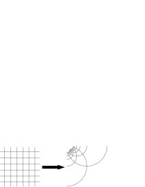
Figure 2.1: A conformal tranformation changes the distances between points on the world-sheet by a local rescaling of the metric without altering the angles between the lines.

We can now turn to analyse the conditions for the theory to remain conformal at quantum level. A preliminary step towards this direction consists in computing the response of (2.1) to a general variation $\delta g_{\alpha\beta}$ of the intrinsic metric:

$$\delta S=\int d\sigma d\tau\frac{\delta S}{\delta g_{\alpha\beta}}\delta g_{\alpha\beta}=\int d\sigma d\tau\sqrt{g}T^{\alpha\beta}\delta g_{\alpha\beta}.$$ (2.9)

$\delta S$ defines the stress tensor (in Euclidean signature for the intrinsic metric):

$$T_{\alpha\beta}=\frac{4\pi}{\sqrt{g}}\frac{\delta S}{\delta g^{\alpha\beta}},$$ (2.10)

the factor $4\pi$ in the definition simplifies its explicit form, that we are going to obtain.

Whenever the action is invariant under a subgroup of all possible variations of the intrinsic metric, the stress tensor will in correspondence enjoy a specific property.

To be specific, for an infinitesimal conformal transformation $\delta g_{\alpha\beta}=\epsilon g_{\alpha\beta}$, the variation of the Action yields

$$\delta S=\frac{1}{4\pi}\int d\sigma d\tau\sqrt{g}T^{\alpha\beta}\ g_{\alpha\beta}\ \epsilon,$$ (2.11)

and thus the vanishing of $\delta S$ asks for the vanishing of the trace of the stress tensor, $T^{\alpha}_{\alpha}=0$.

The most general local variation of the intrinsic metric corresponds to a world-sheet diffeomorphism, and if the Action is invariant under diffeomorphisms, the stress tensor is conserved, $\nabla^{\alpha}T_{\alpha\beta}=0$.

Let us consider the world-sheet Action (2.1) for the class of backgrounds where $B_{\mu\nu}=0$ and the dilaton is constant $\nabla_{\mu}\phi=0$, and compute the stress tensor. The response of the Action to a variation of the intrinsic metric gives:

$$\delta S=\frac{1}{4\pi\alpha^{\prime}}\int d\sigma d\tau\left(\delta(\sqrt{g})g^{\alpha\beta}+\sqrt{g}\delta g^{\alpha\beta}\right)G_{\mu\nu}\partial_{\alpha}X^{\mu}\partial_{\beta}X^{\nu},$$ (2.12)

and thus, by using $\delta(\sqrt{g})=\frac{1}{2}\sqrt{g}\delta g_{\rho\sigma}g^{\rho\sigma}$ one gets

$$T_{\alpha\beta}=\frac{4\pi}{\sqrt{g}}\frac{\delta S}{\delta g^{\alpha\beta}}=\frac{1}{\alpha^{\prime}}\left(\partial_{\alpha}X^{\mu}\partial_{\beta}X^{\nu}-\frac{1}{2}g_{\alpha\beta}\partial_{\gamma}X^{\mu}\partial^{\gamma}X^{\nu}\right)G_{\mu\nu}.$$ (2.13)

A conformal transformation is a particular kind of (world-sheet) diffeomorphism, and the metric on the world-sheet can be chosen to be conformally flat, therefore we can always take a flat metric $\eta_{\alpha\beta}$ as a reference metric for the classical action. Conformal invariance asks for $T^{\alpha}_{\alpha}=0$, while, for a flat reference metric, diffeomorphism invariance imposes $\partial^{\alpha}T_{\alpha\beta}=0$. In complex coordinates $T^{\alpha}_{\alpha}=0$ translates into $T_{z\bar{z}}=0$ and in this case $\partial^{\alpha}T_{\alpha\beta}=0$ yields $\bar{\partial}T_{zz}=0$ and $\partial T_{\bar{z}\bar{z}}=0$, which mean that $T_{zz}=T(z)$ is a holomorphic function and $T_{\bar{z}\bar{z}}=\bar{T}(\bar{z})$ is antiholomorphic.

After quantisations of the two-dimensional theory in the flat reference metric, conformal invariance will demand the same analiticity properties for the stress tensor to hold at the quantum level as well.

In order to detect which are the backgrounds that preserve conformal invariance at the quantum level on the world-sheet sigma model (2.1), one can employ a background field method in the two dimensional field theory, by writing the string coordinates $X^{\mu}=X^{\mu}_{cl}+\xi^{\mu}$, where $X^{\mu}_{cl}$ is the centre of mass string coordinate and $\xi^{\mu}$ is a quantum fluctuation of the order of the string length $\sqrt{\alpha^{\prime}}$. Then the computation of the beta functions for the two dimensional couplings gives a perturbative expansion in the string length $\sqrt{\alpha^{\prime}}$ [10], that at the leading order in $\alpha^{\prime}$ have the form

$$\beta_{\mu\nu}^{G} = \alpha^{\prime}\left(R_{\mu\nu}-\frac{1}{4}H_{\mu\rho\sigma}H_{\nu}^{\rho\sigma}+\nabla_{\mu}\nabla_{\nu}\phi\right)+O(\alpha^{\prime 2})$$

$$\beta_{\mu\nu}^{B} = \alpha^{\prime}\nabla^{\rho}\left(e^{-\phi}H_{\mu\nu\rho}\right)+O(\alpha^{\prime 2})$$

$$\beta_{\mu\nu}^{\phi} = D-26+3\alpha^{\prime}\left[(\nabla\phi)^{2}-R+\frac{1}{12}H^{2}\right]+O(\alpha^{\prime 2})$$ (2.14)

where $H_{\mu\nu\rho}=\partial_{\mu}B_{\nu\rho}+\partial_{\nu}B_{\rho\mu}+\partial_{\rho}B_{\mu\nu}$.

The previous equations show the existence of a large class of spacetimes that at the leading order satisfy Einstein vacuum equations and, quite interestingly, these equations predict the number of spacetime dimensions where the bosonic string can fluctuate to be $D=26$, called the critical dimension. However, the critical string is not the only possibility, since by picking up an arbitrary number of dimensions one can still obtain conformal invariance by adding to the coordinate fields the world-sheet metric scale factor, that in this case does not decouple, and it represents an extra coordinate in the quantum theory. This last possibility goes under the name of non-critical string.

Remaining in the critical dimension $D=26$, the two-dimensional theory (2.1) for general background fields $G_{\mu\nu}(X)$, $B_{\mu\nu}(X)$ and $\phi(X)$ is a non linear sigma model for which a perturbative quantisation is hard to obtain. Let us therefore consider the simpler case where the action is free, corresponding to a flat spacetime metric $G_{\mu\nu}(X)=\eta_{\mu\nu}$, $B_{\mu\nu}=0$ and $\phi$ coordinate independent.

These flat spacetimes are indeed exact conformal backgrounds, since higher order corrections in $\alpha^{\prime}$ to the condition for conformal invariance for the sigma model depend on complicate expressions of the Riemann tensor $R_{\mu\nu\rho\sigma}$, the field strength $H_{\mu\nu\rho}$ and derivatives of the dilaton $\phi$ [11, 12, 13]. These contributions are therefore vanishing for the class of flat spacetimes that we are presently considering.

The world-sheet action (2.1) for this choice of background is given by

$$S=\frac{1}{4\pi\alpha^{\prime}}\int_{\Sigma}d\sigma d\tau\eta_{\mu\nu}\partial_{\alpha}X^{\mu}\partial^{\alpha}X^{\nu}+\chi_{g}\phi$$ (2.15)

where $\chi_{g}$ is the Euler characteristic of the world-sheet

$$\chi_{g}=\frac{1}{8\pi}\int_{\Sigma}d\sigma d\tau\sqrt{g}R^{(2)}=2-2g,$$ (2.16)

and is an integer number that depends on the topology of the world-sheet, $g$ is the genus of the two-dimensional surface, and is given by the number of handles $h$ of the closed surface.

A closed string propagating freely on a flat spacetime describes an infinite cylinder $0\leq\sigma<2\pi$, $-\infty<\tau<\infty$. Quantisation of the two dimensional theory can be worked out after an Euclidean rotation on the surface, so that the coordinate on the cylinder are complexified $w=\sigma-it$. Through the conformal transformation $z=e^{iw}$ we can map the cylinder into the Riemann sphere $\mathcal{S}^{2}=\{\mathbb{C}\cup\{\infty\}\}$, the complex plane together with the points at infinite that have been identified, as shown in fig. 2.2.

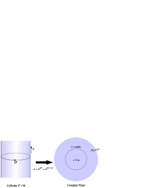
Figure 2.2: The conformal transformation $z=e^{iw}$ maps the cylinder into the Riemann sphere $\mathcal{S}^{2}=\{\mathbb{C}\cup\{\infty\}\}$, the complex plane together with the points at infinite that have been identified.

Constant time slices $t=t_{0}$ on the cylinder are conformally mapped into the circles $C=\{z=e^{i\sigma+t_{0}}\}$ centered in the origin of the complex plane and with radius $e^{t_{0}}$. Hence time grows radially on the plane and the origin corresponds to $t=-\infty$ on the cylinder.

At the tree level we can therefore consider the world-sheet to be the Riemann sphere fig. (2.3) with the action given by the dynamical term in (2.15)

$$S=\frac{1}{2\pi\alpha^{\prime}}\int dzd\bar{z}\eta_{\mu\nu}\partial X^{\mu}\bar{\partial}X^{\nu},$$ (2.17)

whose classical equations of motion are

$$\frac{\delta S}{\delta X_{\mu}}=\frac{1}{\pi\alpha^{\prime}}\bar{\partial}\partial X^{\mu}=0.$$ (2.18)

As a result $\partial X^{\mu}$ is a holomorphic function and $\bar{\partial}X^{\mu}$ is anti-holomorphic.

In the quantised theory the product of fields at coincident points is singular and the equations of motion are violated at such coincident points. This can be easily understood by the following formal relation for the Euclidean path integral on the Riemann sphere

$$0=\int\mathcal{D}X\frac{\delta}{\delta X_{\nu}(z,\bar{z})}\left(X^{\mu}(z^{\prime},\bar{z}^{\prime})e^{-S}\right)$$

$$=\int\mathcal{D}X\left(\eta^{\mu\nu}\delta(z-z^{\prime},\bar{z}-\bar{z}^{\prime})-X^{\mu}(z^{\prime},\bar{z}^{\prime})\frac{1}{\pi\alpha^{\prime}}\bar{\partial}\partial X^{\nu}(z,\bar{z})\right)e^{-S}.$$ (2.19)

The equations of motion are therefore satisfied except at the contact points:

$$X^{\mu}(z^{\prime},\bar{z}^{\prime})\bar{\partial}\partial X^{\nu}(z,\bar{z})=\pi\alpha^{\prime}\eta^{\mu\nu}\delta(z-z^{\prime},\bar{z}-\bar{z}^{\prime}).$$ (2.20)

Using the well known Green Function for the Laplace operator in two dimensions $\bar{\partial}\partial\ln(|z|^{2})=2\pi\delta(z,\bar{z})$, one gets

$$X^{\mu}(z^{\prime},\bar{z}^{\prime})X^{\nu}(z,\bar{z})=\frac{\alpha^{\prime}}{2}\eta^{\mu\nu}ln(|z-z^{\prime}|^{2}).$$ (2.21)

Acting with $\partial=\partial_{z}$ and $\partial^{\prime}=\partial_{z^{\prime}}$ on the previous equation one also obtains another useful relation

$$\partial^{\prime}X^{\mu}(z^{\prime})\partial\ X^{\nu}(z)=-\frac{\alpha^{\prime}}{2}\frac{\eta^{\mu\nu}}{(z-z^{\prime})^{2}}.$$ (2.22)

Before showing the use of the above operator product expansion (OPE), it is convenient to expand the holomorphic function $\partial X^{\mu}(z)$ in Laurent series:

$$\partial X^{\mu}=\sqrt{\frac{\alpha^{\prime}}{2}}\sum_{n=-\infty}^{\infty}z^{-n-1}\alpha^{\mu}_{n}$$ (2.23)

and similarly:

$$\bar{\partial}X^{\mu}=\sqrt{\frac{\alpha^{\prime}}{2}}\sum_{n=-\infty}^{\infty}\bar{z}^{-n-1}\tilde{\alpha}^{\mu}_{n}.$$ (2.24)

The inverse relations are then

$$\alpha^{\mu}_{n} = \sqrt{\frac{2}{\alpha^{\prime}}}\oint_{C}\frac{dz}{2i\pi}z^{n}\partial X^{\mu}(z)$$

$$\tilde{\alpha}^{\mu}_{n} = -\sqrt{\frac{2}{\alpha^{\prime}}}\oint_{C}\frac{d\bar{z}}{2i\pi}\bar{z}^{n}\bar{\partial}X^{\mu}(\bar{z}),$$ (2.25)

where the integration contour $C$ winds the origin.

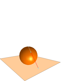
Figure 2.3: Stereographic projection of a sphere into a plane. The north pole is projected to the points at infinite of the plane. Therefore a sphere is equivalent to the complex plane with the points at infinite identificated (Riemann Sphere).

From the world-sheet current $1/\alpha^{\prime}\cdot\partial_{\alpha}X^{\mu}$, associated to the spacetime momentum operator $\partial_{\mu}=1/\alpha^{\prime}\cdot\partial_{\alpha}X^{\mu}\partial_{\alpha}$, one can obtain the correspondent Noether charge by performing contour integral

$$p_{\mu}=\frac{1}{\alpha^{\prime}}\left(\oint_{C}\frac{dz}{2i\pi}\partial X_{\mu}-\oint_{C}\frac{d\bar{z}}{2i\pi}\bar{\partial}X_{\mu}\right)=-\sqrt{\frac{2}{\alpha^{\prime}}}\alpha_{0\ \mu}$$ (2.26)

where the minus sign takes care of the opposite orientation of the $d\bar{z}$ the contour. The independence of the integrals on the choice of the integration contour on the complex plane reflects the time independence of the Noether charge and thus its conservation.

Due to the singularity of the product (2.22), at the coincident points the modes $\alpha^{\mu}_{n}$ no longer commute in the quantum theory. Their commutator can be easily computed by performing the following contour integrals:

$$[\alpha^{\mu}_{n},\alpha^{\nu}_{m}] = \sqrt{\frac{2}{\alpha^{\prime}}}\oint\frac{dz}{2i\pi}z^{n}\partial_{z}X^{\mu}(z)\sqrt{\frac{2}{\alpha^{\prime}}}\oint\frac{dw}{2i\pi}w^{m}\partial_{w}X^{\nu}(w)$$ (2.27)

$$- \sqrt{\frac{2}{\alpha^{\prime}}}\oint\frac{dw}{2i\pi}w^{m}\partial_{w}X^{\nu}(w)\sqrt{\frac{2}{\alpha^{\prime}}}\oint\frac{dz}{2i\pi}z^{n}\partial_{z}X^{\mu}(z)$$

$$= n\eta^{\mu\nu}\delta_{n+m,0},$$

and shows that the operators $a^{\mu}_{n}=\alpha^{\mu}_{n}/\sqrt{n}$ and $(a^{\mu}_{n})^{{\dagger}}=\alpha^{\mu}_{-n}/\sqrt{n}$ represent an infinite set of ladder harmonic oscillator operators.

Integration of (2.23) and (2.24) then gives the normal mode expansion for the coordinates

$$X^{\mu}(z,\bar{z})=x^{\mu}+\frac{\alpha^{\prime}}{2}p^{\mu}\ln(z\bar{z})-\sqrt{\frac{\alpha^{\prime}}{2}}\sum_{n\neq 0}\left(\frac{z^{-n}}{n}\alpha^{\mu}_{n}+\frac{\bar{z}^{-n}}{n}\tilde{\alpha}^{\mu}_{n}\right),$$ (2.28)

where $p^{\mu}$ is the spacetime momentum of the centre of mass of the string.

Let us return to the stress tensor that reads

$$T_{zz}=T(z)=\frac{1}{\alpha^{\prime}}\partial X^{\mu}(z,\bar{z})\partial X_{\mu}(z,\bar{z}).$$ (2.29)

Eq. (2.22) says that this expression is ill-defined and needs to be regularized by subtracting its divergence at the coincidence points

$$T(z)=\frac{1}{\alpha^{\prime}}:\partial X^{\mu}(z,\bar{z})\partial X_{\mu}(z,\bar{z}):=\frac{1}{\alpha^{\prime}}\partial X^{\mu}(z,\bar{z})\partial X_{\mu}(u,\bar{u})-\frac{D}{2(z-u)^{2}}$$ (2.30)

We are interested at the OPE of the stress tensor with itself since, as we will show, the knowledge of the singularities in the product $T(z)T(w)$ is crucial in order to reconstruct the quantum version of the classical conformal algebra (2.8).

In order to compute $T(z)T(u)$ we use its regularized definition (2.30) and the OPE in (2.22). The computation gives

$$T(z)T(u)=:\frac{1}{\alpha^{\prime}}\partial X^{\mu}(z,\bar{z})\partial X_{\mu}(z^{\prime},\bar{z}^{\prime})::\frac{1}{\alpha^{\prime}}\partial X^{\rho}(u,\bar{u})\partial X_{\rho}(u^{\prime},\bar{u}^{\prime}):$$

$$=\frac{\eta^{\mu}_{\mu}/2}{(z-u)^{4}}+\frac{2T(u)}{(z-u)^{2}}+\frac{\partial T(u)}{(z-u)}=\frac{D/2}{(z-u)^{4}}+\frac{2T(u)}{(z-u)^{2}}+\frac{\partial T(u)}{(z-u)}.$$ (2.31)

The Laurent coefficients $L_{n}$ in the stress tensor expansion define the Virasoro operators

$$T_{zz}(z)=T(z)=\sum_{n}z^{-n-2}L_{n}\qquad T_{\bar{z}\bar{z}}(\bar{z})=\bar{T}(\bar{z})=\sum_{n}\bar{z}^{-n-2}\bar{L}_{n}.$$ (2.32)

Since the stress tensor is the Noether current for the conformal symmetry we can compute the generators of the conformal transformations by integrating the current on a constant time slice

$$L_{n}=\frac{1}{2\pi i}\oint_{C}dzz^{n+1}T(z),$$ (2.33)

and similarly for the generators $\bar{L}_{n}$ of the antiholomorphic copy of the conformal algebra

$$\bar{L}_{n}=-\frac{1}{2\pi i}\oint_{C}d\bar{z}\bar{z}^{n+1}\bar{T}(\bar{z}).$$ (2.34)

Finally, through the OPE (2.31) and the relation (2.33) we can compute the quantum version of the the conformal algebra

$$[L_{n},L_{m}]=(n-m)L_{n+m}+\frac{D}{12}n(n-1)(n+1)\delta_{n+m,0}.$$ (2.35)

An identical relation holds for the anti-holomorphic Virasoro operators $\bar{L}_{n}$. This is called the Virasoro algebra $\mathcal{V}$. Comparison with eq. (2.8) for the classical commutators shows that the quantisation of the theory introduces a central extension in the conformal algebra. Indeed the number of spacetime dimensions $D$ that appears on the right hand-side corresponds to what is called the central charge of the the Virasoro algebra, and signals the presence of a conformal anomaly. In the covariant path integral quantisation for the bosonic string, the symmetries ask for the introductions of woldsheet ghost fields that contribute themselves to the stress tensor and therefore to the central charge in the Virasoro algebra. In this approach, imposing conformal invariance at quantum level asks for the cancellation of the conformal anomaly, a condition that constraints the number of coordinate fields to be $D_{crit}=26$, this number is called the spacetime critical dimension.

In the two dimensional quantum CFT there is an important correspondence between states and operators that allows to classify the representations of the Virasoro algebra. At the end of the day, the string excitations carry a representation of the Virasoro algebra, so this analysis is useful to classify the states in the string spectrum.

Once one has identified an asymptotic inner ($z=0$ on the sphere or $t=-\infty$ on the cylinder) ground state $|0\rangle$, one can obtain a generic asymptotic inner state $|f\rangle$ by acting with a field $f(0)$ on the ground state $|f\rangle=f(0)|0\rangle$.

For example, the string ground state with center of mass momentum $k_{\mu}$ is given by $e^{ik_{\mu}X^{\mu}(0)}|0\rangle=|0,k_{\mu}\rangle$.

Similarly, for an excited state $\alpha^{\mu}_{-n}\tilde{\alpha}^{\nu}_{-n}|0\rangle$ one has

$$\alpha^{\mu}_{-n}\tilde{\alpha}^{\nu}_{-n}|0\rangle=\frac{2}{\alpha^{\prime}}\oint\frac{dz}{2i\pi}z^{n}\partial X^{\mu}(z)\oint\frac{d\bar{z}}{2i\pi}\bar{z}^{n}\bar{\partial}X^{\nu}(z)|0\rangle.$$ (2.36)

Expanding $\partial X^{\mu}(z)$($\bar{\partial}X^{\nu}(\bar{z})$) around $z=0(\bar{z}=0)$,

$$\partial X^{\mu}(z)=\partial X^{\mu}(0)+...+\frac{z^{n-1}}{(n-1)!}\partial^{n}X^{\mu}(0)+...,$$ (2.37)

and performing the contour integrals, one gets

$$\alpha^{\mu}_{-n}\tilde{\alpha}^{\nu}_{-n}|0\rangle=\frac{2}{\alpha^{\prime}(n-1)!(n-1)!}\partial^{n}X^{\mu}(0)\bar{\partial}^{n}X^{\nu}(0)|0\rangle,$$ (2.38)

that shows a general correspondence between inner states and fields at $z=0$.

States created at a generic point $z_{0}$ on the sphere and carring momentum $k$ are then associated to the operator

$$\frac{2}{\alpha^{\prime}}e^{ik_{\mu}X^{\mu}(z_{0},\bar{z}_{0})}\partial^{n}X^{\mu}(z_{0})\bar{\partial}^{n}X^{\nu}(\bar{z_{0}}).$$ (2.39)

Let us see which kind of constraints the conformal algebra imposes on an operator of this kind and therefore on the correspondent quantum state.

From the Virasoro algebra in (2.35), it is clear that the only subalgebra that survives quantisation is generated by $(L_{1},L_{0},L_{-1})$, because for $n=-1,0,1$ the central charge contribution vanishes. This algebra is isomorphic to $SL(2,\mathbb{R})$ and, together with the anti-holomorphic counterpart, forms the algebra $SL(2,\mathbb{C})=SL(2,\mathbb{R})\oplus SL(2,\mathbb{R})$.

$SL(2,\mathbb{C})$ is the only subalgebra of the conformal algebra whose transformations map the Riemann sphere into itself, in particular ${L}_{0}=z\partial$ generates a constant scale transformations $z\rightarrow\lambda z$ for $\lambda\in\mathbb{C}$. Therefore to respect the unbroken $SL(2,\mathbb{C})$ symmetry a generic operator

$$\frac{2}{\alpha^{\prime}}\int dzd\bar{z}e^{ik_{\mu}X^{\mu}(z,\bar{z})}\partial^{n}X^{\nu}(z)\bar{\partial}^{n}X^{\mu}(\bar{z})$$ (2.40)

must be ${L}_{0}$ invariant.

Since the integration measure on the sphere scales as $dzd\bar{z}\rightarrow|\lambda|^{2}dzd\bar{z}$, the operator itself needs to scale oppositely for the integral (2.40) to be $SL(2,\mathbb{C})$ invariant.

The operators $f(z,\bar{z})$ that create physical states need to have definite global scaling properties. This kind of operators are called primaries with conformal weights $(h,\bar{h})$, ($h$ and $\bar{h}$ real numbers), if under the dilatation $z\rightarrow\lambda z$ they transform as $f(\lambda z,\bar{\lambda}\bar{z})=\lambda^{-h}\bar{\lambda}^{-\bar{h}}f(z)$.

With this definition in mind it is clear that

$$\int dzd\bar{z}V(z,\bar{z}),$$ (2.41)

is $L_{0}$ invariant only if $V(z,\bar{z})$ has conformal weights $(1,1)$. This implies that physical asymptotic states are created by $(1,1)$ operators, i.e.

$$L_{0}|phys\rangle=|phys\rangle\qquad\bar{L}_{0}|phys\rangle=|phys\rangle.$$ (2.42)

Let us consider the rank-two tensor operator

$$\int dzd\bar{z}e^{ik_{\mu}X^{\mu}(z,\bar{z})}\partial X^{\mu}(z)\bar{\partial}X^{\nu}(\bar{z})$$ (2.43)

$\partial X^{\mu}(z)\bar{\partial}X^{\nu}(\bar{z})$ has classical $(1,1)$ scaling properties due to the presence of the derivatives $\partial$ and $\bar{\partial}$ and $(1,1)$ conformal weights, as we can check by computing $\left[L_{0},\partial X^{\mu}(0)\right]=\alpha^{\prime}\partial X^{\mu}(0)$ with the help of (2.33) and (2.22). A similar computation shows instead that $e^{ik_{\mu}X^{\mu}(z,\bar{z})}$ has conformal weights $(\alpha^{\prime}k^{2}/2,\alpha^{\prime}k^{2}/2)$ ( note that classically this operators has zero scaling dimension a property that we recover in the limit $\alpha^{\prime}\rightarrow 0$). $SL(2,\mathbb{C})$ invariance for the rank-two tensor operator therefore implies that the sum of the conformal weights of $\partial X^{\mu}(z)\bar{\partial}X^{\nu}(\bar{z})$ and $e^{ik_{\mu}X^{\mu}(z,\bar{z})}$ be equal to $(1,1)$

$$(\alpha^{\prime}k^{2}/2+1,\ \alpha^{\prime}k^{2}/2+1)=(1,1),$$ (2.44)

which happens only if $k^{2}=-m^{2}=0$   i.e. only if the operator creates massless states.

These states need to carry an irreducible representation of the spacetime Lorentz group and the decomposition of the rank two tensor gives the spin two symmetric traceless part that we identify with the graviton $G_{\mu\nu}$, the antisymmetric part $B_{\mu\nu}$ and the trace part $\phi$, the dilaton.

Note that operators like $e^{ik_{\mu}X^{\mu}(z,\bar{z})}\partial^{n}X^{\mu}\bar{\partial}^{m}X^{\nu}$ for $m$ different from $n$ cannot create physical states since even at non zero mass they cannot respect the $SL(2,\mathbb{C})$ symmetry, whence for $n$ equal to $m$ and with a non vanishing mass they can respect this symmetry. This is an example of a level matching constraint, which in general means that the state

$$e^{ik_{\mu}X^{\mu}(0,0)}\partial^{n_{1}}X^{\mu_{1}}(0)\bar{\partial}^{\tilde{n}_{1}}X^{\nu_{1}}(0)...\partial^{n_{p}}X^{\mu_{p}}(0)\bar{\partial}^{\tilde{n}_{p}}X^{\nu_{p}}(0)|0\rangle$$

$$\sim\alpha^{\mu_{1}}_{-n_{1}}\tilde{\alpha}^{\nu_{1}}_{-\tilde{n}_{1}}...\alpha^{\mu_{p}}_{-n_{p}}\tilde{\alpha}^{\nu_{p}}_{-\tilde{n}_{p}}|k,0\rangle$$ (2.45)

needs to satisfy the level matching condition

$$n_{1}+...n_{p}=\tilde{n}_{1}+...+\tilde{n}_{p},$$ (2.46)

in order to respect the $SL(2,\mathbb{C})$ and therefore to by physical.

In this case, the physical states created by (2.45) have mass

$$m^{2}=-k^{2}=\frac{2}{\alpha^{\prime}}(n_{1}+...+n_{p}-1).$$ (2.47)

To summarise, $SL(2,\mathbb{C})$ invariance implies that only operators with well defined scaling properties (conformal weights) can create asymptotic physical states. There is a precise relation between the rank of tensor operators and the mass of the corresponding physical states. In particular, the scalar groundstate $e^{ik_{\mu}X_{\mu}(z,\bar{z})}|0\rangle$, has conformal weights $(\alpha^{\prime}k^{2}/2,\alpha^{\prime}k^{2}/2)$ and thus it represents a tachyon $m^{2}=-2/\alpha^{\prime}$. The only massless states are those created by the rank-two tensor: the metric $G_{\mu\nu}$ the antisymmetric tensor $B_{\mu\nu}$ and the dilaton $\phi$. All higher rank tensors that respect level matching create massive states.

The quatization of the bosonic string presents some subtleties related to the Lorentzian signature of the space-time metric. In fact, one can see from (2.27), that the oscillator modes associated with the time coordinate $X^{0}$ satisfy a wrong sign commutation relation, and thus create negative-norm quantum states.

There are various routes to deal with this problem that correspond to different, but at the end equivalent, ways to quantise the theory. At the classical level, the equations of motion for the world-sheet metric yield the constraint $T_{\alpha\beta}=0$. There are two alternative ways to proceed with the quantisation: one can impose the $T_{\alpha\beta}=0$ constraint before quantisation, reducing in this way the number of variables that describe the string degrees of freedom, or one can quantise the whole $X^{\mu}$ and impose the constraint in a operator form on the quantum states. In the first case the quantisation is worked out in a gauge in which the oscillators satisfying wrong sign commutation relations are not dynamical, because they are expressed in terms of the transverse oscillators via the solution of the classical constraint. However D-dimensional Lorentz covariance is not manifest and it is recovered only for $D=26$. This needs to be checked by verifying the proper commutation relations for the Lorentz generators, constructed with a reduced number of oscillators.

In the second case all coordinates are quantised in a manifestly covariant way, but the absence of negative norm states in the spectrum then follows by imposing the constraints in a operatorial form on the physical states. Also in this case the Hilbert space is indeed free of nagative-norm states again only if $D=26$.

Here we follow the most economic way to derive the physical spectrum by introducing light cone coordinates

$$X^{\pm}=\frac{1}{\sqrt{2}}(X^{0}\pm X^{1}),$$ (2.48)

a choice manifestly non covariant. One can choose a gauge that allows to solve the constraints in terms of the dangerous longitudinal oscillators. In such a gauge $X^{+}$ is identified with the world-sheet time $\tau$, a choice that is indeed possible because every conformal transformation is induced by a change of coordinates on the world-sheet that satisfies the Laplace equation as we have shown in eq. (2.5) and the equation of motion for $X^{+}$ is precisely the same equation:

$$\partial^{\alpha}\partial_{\alpha}X^{+}=0.$$ (2.49)

With this choice

$$X^{+}=x^{+}+\frac{\alpha^{\prime}}{2}p^{+}\ln(z\bar{z})=x^{+}-\sqrt{\frac{\alpha^{\prime}}{2}}\alpha^{+}_{0}\ln(z\bar{z})$$ (2.50)

we have set to zero the oscillations along the $X^{+}$ directions, $\alpha_{n}^{+}=0$. This is quite natural since oscillations along the world-sheet are expected not to be physical due to (world-sheet) reparametrization invariance.

The classical constraints $L_{n}=0$ then eliminate the non-dynamical variables. Indeed

$$L_{n} = \oint_{C}\frac{dz}{2\pi i}z^{n+1}T(z)=\frac{1}{\alpha^{\prime}}\oint_{C}\frac{dz}{2\pi i}z^{n+1}:\partial X^{\mu}\partial X_{\mu}(z):$$ (2.51)

$$= \frac{1}{2}\oint_{C}\frac{dz}{2\pi i}z^{n+1}:\sum_{m=-\infty}^{\infty}z^{-m-1}\alpha_{m}^{\mu}\sum_{l=-\infty}^{\infty}z^{-l-1}\alpha_{l\ \mu}:$$

$$= \frac{1}{2}\sum_{m=-\infty}^{\infty}\alpha_{-m+n}^{\mu}\alpha_{m\ \mu},$$

and in the lightcone gauge (2.50)

$$0=L_{n}=\sum_{m=-\infty}^{\infty}\alpha_{-m+n}^{+}\alpha_{m}^{-}-\frac{1}{2}\sum_{m=-\infty}^{\infty}\alpha_{-m+n}^{i}\alpha_{m}^{i}=\frac{1}{2}\alpha_{0}^{+}\alpha_{n}^{-}-\frac{1}{2}\sum_{m=-\infty}^{\infty}\alpha_{-m+n}^{i}\alpha_{m}^{i}$$ (2.52)

allow to express the $\alpha_{n}^{-}$ in terms of the physical transverse oscillators:

$$\alpha_{n}^{-}=\frac{1}{2\alpha_{0}^{+}}\sum_{m=-\infty}^{\infty}\alpha_{-m+n}^{i}\alpha_{m}^{i}=-\frac{1}{\sqrt{2\alpha^{\prime}}p^{+}}\sum_{m=-\infty}^{\infty}\alpha_{-m+n}^{i}\alpha_{m}^{i}.$$ (2.53)

Thus showing that only the oscillations transverse to the world-sheet are physical with a positive-definite scalar product. A closed string state is therefore described in the lightcone gauge by a $D$-dimensional center of mass momentum $p^{\mu}$, and its oscillations are created by $D-2$ transverse bosonic oscillators $\alpha^{i}_{n<0}=\sqrt{-n}(a^{i}_{-n})^{{\dagger}}$

$$e^{ik_{\mu}X^{\mu}(0,0)}\partial^{n_{1}}X^{i_{1}}(0)\bar{\partial}^{\tilde{n}_{1}}X^{j_{1}}(0)...\partial^{n_{p}}X^{i_{p}}(0)\bar{\partial}^{\tilde{n}_{p}}X^{j_{p}}(0)|0\rangle$$ (2.54)

$$\sim\alpha^{i_{1}}_{-n_{1}}\tilde{\alpha}^{j_{1}}_{-\tilde{n}_{1}}...\alpha^{i_{p}}_{-n_{p}}\tilde{\alpha}^{j_{p}}_{-\tilde{n}_{p}}|k^{\mu},0\rangle.$$

These states satisfy the level matching condition

$$n_{1}+...+n_{p}=\tilde{n}_{1}+....+\tilde{n}_{p}$$ (2.55)

and have a mass

$$m^{2}=-k^{2}=\frac{1}{\alpha^{\prime}}\left[2(n_{1}+...+n_{p})-2\right].$$ (2.56)

Consistency with D-dimensional Lorentz symmetry requires for the tensor field operator (2.54) to create states carrying a representation of the little group of $SO(1,D-1)$. Massless states needs to be in irreducible representation of $SO(D-2)$, while massive states in $SO(D-1)$ ones.

As a consequence of $SL(2,\mathbb{C})$ invariance the only massless states in the closed string spectrum are those created by the rank-two $(1,1)$ tensor field

$$\frac{2}{\alpha^{\prime}}e^{ik_{\mu}X^{\mu}(0,0)}\partial X^{i}(0)\bar{\partial}X^{j}(0)|0\rangle=\alpha^{i}_{-1}\tilde{\alpha}^{j}_{-1}|k_{\mu},0\rangle\qquad i=1,...,D-2.$$ (2.57)

These states correspond to the decomposition of the rank-two tensor field into $SO(D-2)$ irreducible representations

$$(D-2)^{2}=\left(\frac{(D-2)(D-1)}{2}-1\right)+\frac{(D-2)(D-3)}{2}+1.$$ (2.58)

Clearly, the $(D-2)^{2}$ degrees of freedom do not fit into a sum of two-tensor irreducible representations of $SO(D-1)$

$$(D-1)^{2}=\left(\frac{(D-1)D}{2}-1\right)+\frac{(D-1)(D-2)}{2}+1.$$ (2.59)

In other worlds, consistency with Lorentz covariance requires for the states created by the rank-two tensor to be massless.

For massive states, created by Higher-rank tensors operators, the situation is different and the number of degrees of freedom fits in producing a decomposition in terms of $SO(D-1)$ irreducible representations. This is possible because there is more then one operator that coresponds to a given conformal weight. For example, there are two operators with $(2,2)$ weights

$$\partial X^{i_{1}}(0)\partial X^{i_{2}}(0)\bar{\partial}X^{j_{1}}(0)\bar{\partial}X^{j_{2}}(0)\qquad\partial^{2}X^{i_{1}}(0)\bar{\partial}^{2}X^{j_{1}}(0),$$ (2.60)

which give rise to $(D-2)^{4}+(D-2)^{2}$ degrees of freedom for the first closed string massive level. It is possible to show that this number equals a sum of $SO(D-1)$-irreducible representations, and that actually this is the case for the full list of primary fields, in agreement with the Lorentz symmetry.

The condition dictated by both $SL(2,\mathbb{C})$ and $SO(1,D-1)$ invariance on the states created by the rank-two tensor operator actually is satisfied only if the number of spacetime dimension is $D=26$.

Let us consider the expression for $L_{0}$ in terms of lightcone oscillators eq. (2.51)

$$L_{0}=\frac{1}{2}\sum_{m=-\infty}^{\infty}\alpha_{-m}^{\mu}\alpha_{m\ \mu}=\frac{1}{2}\sum_{m=-\infty}^{-1}\alpha_{-m}^{i}\alpha_{m}^{i}+\frac{\alpha_{0}^{2}}{2}+\frac{1}{2}\sum_{m=1}^{\infty}\alpha_{-m}^{i}\alpha_{m}^{i}$$ (2.61)

with $\alpha_{0}^{2}=2\alpha_{0}^{+}\alpha_{0}^{-}-\alpha_{0}^{i}\alpha_{0}^{i}=\alpha^{\prime}/2\cdot p^{2}$. The first term of the last r.h.s. needs to be normal ordered, so that

$$\sum_{m=-\infty}^{-1}\alpha_{-m}^{i}\alpha_{m}^{i}=\sum_{m=1}^{\infty}\alpha_{-m}^{i}\alpha_{m}^{i}+\frac{D-2}{2}\sum_{m=1}^{\infty}m$$ (2.62)

and

$$L_{0}=\frac{\alpha_{0}^{2}}{2}+\sum_{m=1}^{\infty}\alpha_{-m}^{i}\alpha_{m}^{i}+\frac{D-2}{2}\sum_{m=1}^{\infty}m.$$ (2.63)

The divergent sum can be regularised by inserting a smooth cutoff

$$\sum_{m=1}^{\infty}m\rightarrow\sum_{m=1}^{\infty}me^{-m\epsilon}=\frac{1}{\epsilon^{2}}-\frac{1}{12}+O(\epsilon)$$ (2.64)

In this way the normal ordered expression for $L_{0}$ reads:

$$L_{0}=\frac{\alpha_{0}^{2}}{2}+\sum_{m=1}^{\infty}\alpha_{-m}^{i}\alpha_{m}^{i}-\frac{D-2}{24}=\frac{\alpha^{\prime}}{2}p^{2}+\sum_{m=1}^{\infty}m(a_{m}^{i})^{{\dagger}}a_{m}^{i}-\frac{D-2}{24}$$ (2.65)

and thus the first excited states are massless only if $D=26$.

We have seen that conformal invariance at tree level requires that operators associated to physical string excitations have conformal weights equal to $(1,1)$. This in turn determines the mass of the associated states. In the CFT language operators with conformal weights $(1,1)$ are called marginal, since at linear order a perturbation induced by them does not break conformal invariance (see below). It follows that all the tree level string states are created by marginal operators.

However, whenever a string state flows in a loop diagram, its momentum can be off-shell. In the UV regime the fluctuations are regulated by the finiteness of the string length, and thus are not UV dangerous. On the other hand, the IR regime is much more subtle, since the fluctuations can induce effects on the background. As we will mention below, zero momentum fluctuations can break conformal invariance and change the infrared (background) properties of the theory.

In the infrared limit $k^{2}\rightarrow 0$, the effect of a fluctuation can be taken into account by adding to the original CFT a perturbation term which corresponds to a variation of the couplings $\lambda_{k}$ (the string background) of primary operators $\mathcal{O}_{h}^{k}$ (the fields whose mode is the fluctuation) of conformal weights $h=\bar{h}$

$$\delta S=\int dzd\bar{z}\ \mathcal{O}_{h}^{k}\delta\lambda_{k}.$$ (2.66)

The beta functions $\beta_{k}$ associated to the couplings $\lambda_{k}$ can be obtained by a perturbative expansion in an increasing number of tree level correlators of the two dimensional theory.

Up to second order in the fluctuations $\delta\lambda_{k}$, the $\beta_{k}$ are calculated to be [20]:

$$\beta_{k}^{(1)} = 2(h-1)\delta\lambda_{k},$$

$$\beta_{k}^{(2)} = c_{k}^{ij}\delta\lambda_{i}\delta\lambda_{i}.$$ (2.67)

The first order $\beta_{k}^{(1)}$ contribution emerges from the OPEs between the primary operators $\mathcal{O}_{h}^{k}$ and the stress tensor $T$ and therefore depends on the conformal weight $h$ of the field. The second order $\beta_{k}^{(2)}$ contribution emerges instead from the OPEs between two primary fields, i.e. from the two point function

$$\mathcal{O}_{h}^{i}(z,\bar{z})\mathcal{O}_{h}^{j}(w,\bar{w})\sim\frac{c^{ij}_{k}}{|z-w|^{2}}\mathcal{O}_{h}^{k}(w,\bar{w})$$ (2.68)

and is therefore quadratic in the perturbation.

From equation (2.67) it is then clear the role played by irrelevant $h>1$, marginal $h=1$ and $h<1$ irrelevant perturbations on the background. Massive string modes with $h>1$ are irrelevant perturbations, since they induce a positive $\beta_{k}^{(1)}$, and therefore their perturbation disappears in the IR with no effect on the background. The ground state $h=-1$ is instead relevant, the beta function is negative so that a perturbation to the original CFT grows in the infrared and changes drastically the background configuration.

For marginal perturbations $h=1$, such as those induced from the infrared fluctuations of the string massless modes, at first order in the fluctuation the beta function vanishes. As an example consider a fluctuation of the metric at zero momentum $\delta G_{\mu\nu}$. At linearised level the beta function is zero, (first equation of (2.67)), so that the theory remains at its critical point.

From the second equation in (2.67), we see that the perturbation can in principle break conformal invariance. The running of the background metric is

$$\frac{\partial}{\partial(ln\Lambda)}G_{\mu\nu}=\beta_{\mu\nu}^{(2)}=C_{\mu\nu}^{\alpha\beta\gamma\delta}\delta G_{\alpha\beta}\delta G_{\gamma\delta}+O(G^{3})$$ (2.69)

where the coefficients $C_{\mu\nu}^{\alpha\beta\gamma\delta}$ are those in the OPE

$$:\partial X^{\alpha}\bar{\partial}X^{\beta}(z,\bar{z})::\partial X^{\gamma}\bar{\partial}X^{\delta}(w,\bar{w}):\sim\frac{C^{\alpha\beta\gamma\delta}_{\mu\nu}}{|z-w|^{2}}:\partial X^{\mu}\bar{\partial}X^{\nu}(w,\bar{w}):$$ (2.70)

that gives the propagator of the graviton on a given background.

In order to have stability for the background one needs therefore to check that the second order beta function is positive so that the perturbation does not affect the IR properties of the theory. Of course for consistency one should check the value of the beta at every order in this non linear perturbative expansion.

String backgrounds compatible with conformal invariance must satisfy the field equations (2.14) that are expressed as a perturbative expansion in the string scale $\alpha^{\prime}$, whose terms involve an increasing number of derivatives of the background fields. In a slow varying field regime the leading order in $\alpha^{\prime}$ can be already a good approximation. This corresponds for example to the case where the string length is much smaller than the scale of variation of the background metric, described by the curvature radius of the manifold on which the string propagates.

Conformal invariance allows to split the string between on-shell classical backgrounds and quantum fluctuations. In general quantum effects spoil the aproximation and infrared tachyonic fluctuations or tadpoles ask for background redefinition. This might be cured if we knew how to shift the vacuum, but the first quantised formulation is restricted on-shell and the off-shell continuation remains unknown. Spacetime supersymmetry represents a partial way out for this problem since it exclude the presence of these destabilization effects. The first step to achieve specetime supersymmetry can be via the introduction of world-sheet spinors and a two dimensional world-sheet supersymmetry. The conformal symmetry gets enlarged into a superconformal symmetry a subject that will be discussed in the next two sections.

2.2 $N=2$ superconformal symmetry and spacetime supersymmetry

It is interesting to see under which assumptions the closed string spectrum exhibits spacetime supersymmetry.

On $D=10$ Minkowski spacetime, as we will discuss in the next section, there are several closed string spectra that exhibit modular invariance, a fundamental constraint that singles out the consistent string spectra discussed in section four. In particular, type IIA and type IIB are supersymmetric, while there are two more theories that have a modular invariant spectrum but with no supersymmetries: type 0A and type 0B. The non-supersymmetric type 0 theories are purely bosonic and are unstable on $D=10$ flat spacetime as the presence of a tachyonic excitation in their spectra suggests.

After compactification the preservation of some spacetime supersymmetries depends on the nature of the compact space. Actually spacetime supersymmetry does not seem to be required by any fundamental principle, rather is the absence of backreaction on the background that singles out the supersymmetric solutions as those that are really tractable in a first quantised formulation. A background giving rise to spacetime supersymmetry and satisfying the $\alpha^{\prime}$ leading order string equations of motion will generally not be destabilised by classical stringy corrections (Higher order in $\alpha^{\prime}$), in the sense that either it remains a solution to all orders of the $\alpha^{\prime}$ corrected background equations of motion or, more generally, some of its geometrical data needs to be corrected in order to keep up with the perturbative correction from the sigma model [11, 12, 13], but these changes do not modify the form of the low energy effective action [24, 25, 26]. Moreover, in the presence of supersymmetry the background cannot be destabilised by loop quantum corrections, since both vacuum diagrams and tadpoles vanish for supersymmetric solutions [27] [28].

Conversely, for non-supersymmetric compactifications both classical string effects (in $\alpha^{\prime}$) and quantum corrections to the vacuum energy (in $g_{s}$) give perturbative corrections to the equations of motion that in most of the cases invalidate the original background as a solution. This cases are rather more complicate then the supersymmetric ones, since order by order in perturbation theory the background receives substantial corrections from the fluctuations. The hope is that taking the supersymmetric solutions as a guide one could find solutions where supersymmetry is hidden (spontaneously broken) with the analytic control of the unbroken phase still present.

Let us study under which conditions the spectrum of states in a world-sheet SCFT (superconformal theory) enjoys spacetime supersymmetry. We will focus to the case of $\mathcal{N}=2$ superconformal symmetry on the world-sheet, actually $\mathcal{N}=(2,2)$ taking into account the holomorphic and anti-holomorphic closed string sectors. As we shall see this is the symmetry possessed by the Neveu-Schwarz Ramond string in the light cone gauge.

The aim of this section is to present the construction of a superconformal algebra and to show which kind of projection on the Hilbert space of states (GSO projection [29] and its generalisations) yields spacetime supersymmetry.

To construct an $\mathcal{N}=2$ superconformal theory, (fixing the attention to the holomorphic sector), besides a conformal symmetry with a stress tensor $T(z)$ that satisfies all the properties illustrated in the previous section, we need to introduce two supercurrents $G^{1}(z)$ and $G^{2}(z)$, that satisfy the OPE [30]

$$T(z)G^{i}(w) \sim \frac{3/2}{(z-w)^{2}}G^{i}(w)+\frac{\partial_{w}G^{i}(w)}{(z-w)},$$

$$G^{1}(z)G^{2}(w) \sim \frac{2c/3}{(z-w)^{3}}\frac{2T(w)}{(z-w)}+i\left(\frac{2j(w)}{(z-w)^{2}}+\frac{\partial_{w}j(w)}{(z-w)}\right)$$ (2.71)

In turn it, this introduces a new $U(1)$ current $j(z)$ appearing in the last of the previous OPEs.
The new current $j(z)$ satisfies

$$T(z)j(w) \sim \frac{j(w)}{(z-w)^{2}}+\frac{\partial_{w}j(w)}{(z-w)}$$

$$j(z)G^{1}(w) \sim \frac{iG^{2}(w)}{(z-w)}$$

$$j(z)G^{2}(w) \sim \frac{-iG^{2}(w)}{(z-w)}$$

$$j(z)j(z) \sim \frac{c/3}{(z-w)}$$ (2.72)

The important point is that the $\mathcal{N}=2$ theories are one-parameter families of isomorphic algebras. The continuous parameter corresponds to the choice of boundary conditions for the supercurrents

$$G^{\pm}(e^{2i\pi}z)=-e^{\mp 2i\pi a}G^{\pm}(z),$$ (2.73)

with $G^{\pm}(z)=\frac{1}{2}(G^{1}(z)\pm iG^{2}(z))$.

For every value of $a=\eta+\frac{1}{2}$, with $0\leq\eta\leq\frac{1}{2}$, the algebras are all isomorphic. This isomorphism can be checked directly by showing that the new operators

$$L_{n}^{\prime} = L_{n}+\eta j_{n}+\frac{c}{6}\eta^{2}\delta_{n,0}$$

$$j_{n}^{\prime} = j_{n}+\eta j_{n}+\frac{c}{3}\eta\delta_{n,0}$$

$$G_{r}^{\pm^{\prime}} = G_{r\pm\eta}^{\pm},$$ (2.74)

generate the same $\mathcal{N}=2$ superconformal algebra.

One can extend the isomorphism to the representations as well, the operation that connects two representation in two different twisted sectors is called spectral flow.

A unitary map that realizes the spectral flow is given explicitly by: $U_{\eta}=e^{-i\sqrt{\frac{c}{3}}\eta\Phi}$ when the U(1) current is bosonised $j(z)=i\sqrt{\frac{c}{3}}\partial_{z}\Phi$. A generic field with a U(1) charge $q$ under $j(z)$ can then be written as

$$f=\hat{f}e^{-i\sqrt{\frac{3}{c}}\Phi},$$ (2.75)

where $\hat{f}$ is U(1) neutral. $f$ creates the state $|f\rangle$, while the twisted state $|f_{\eta}\rangle$ is created by the same field through the map $U_{\eta}fU^{-1}_{\eta}$.

Now, the R and NS sectors can be defined to correspond to the choices $a=0$ and $a=\frac{1}{2}$, for the (2.73) boundary conditions for the supercurrent. Therefore the states in the two sectors are connected by $U_{1/2}$ spectral flow. Of course the OPE between the operator $U_{1/2}$ and $f$ needs to be singular in order to connect $f$ to the corresponding twisted field $f_{\eta}$, otherwise the action of the operator $U_{1/2}$ on the field $f$ would be trivial. From the explicit form of the OPE

$$f(z,\bar{z})U_{\eta}(z,\bar{z})=\hat{f}e^{-i\sqrt{\frac{3}{c}}\Phi(z,\bar{z})}e^{-i\sqrt{\frac{c}{3}}\frac{1}{2}\Phi(w,\bar{w})}\sim|w|^{\frac{q}{2}}e^{-i\left(\sqrt{\frac{3}{c}}-\sqrt{\frac{c}{3}}\right)\Phi(w,\bar{w})}\left[1+O(w,\bar{w})\right],$$ (2.76)

one can see that demanding semilocality in the above expansion corresponds to the restriction $q\in 2\mathbb{Z}+1$. In this case $U_{1/2}$ creates a square-root branch cut on the world-sheet and interchanges spacetime bosons and fermions.

The projection of the $\mathcal{N}=2$ spectrum of the superconformal theory that include both R and NS sectors into states with integer and odd $U(1)$ charge gives rise to spacetime supersymmetry as more careful investigations had proved [31, 32]. This truncation of the spectrum is called the GSO projection. We will reconsider this projection in the specific example of $D=10$ superstring on flat spacetime in the next section and further in the section dedicated to the torus vacuum amplitudes.

In the more general case of orbifold theories, where various twisted sectors may coexist, one needs to workout a similar condition of semilocality for the action of the spectral flow operator. This restricts the allowed $U(1)$ charges for the states, and the spectrum may enjoy spacetime supersymmetry in all cases where a solution of the semilocality condition exists. The corresponding restriction on the $q$ charges represents a generalised GSO projection.

In the above discussion we focused only on the holomorphic sector. Indeed, the bulk SCFT posses $N=(2,2)$ superconformal symmetry. The four world-sheet supercharges, $Q_{L1}(z)$, $Q_{L2}(z)$ from the holomorphic sector and $Q_{R1}(\bar{z})$, $Q_{R2}(\bar{z})$ from the anti-holomorphic one are the zero modes of the $G^{\pm}_{L}(z)$ and $G^{\pm}_{R}(\bar{z})$ supercurrents. If an appropriate GSO projection on the spectrum is performed, than the states of $N=(2,2)$ superconformal theory realize $N=2$ spacetime supersymmetry. The spacetime supercharges are the spectral flow operators (holomorphic and antiholomorphic), constructed by world-sheet quantities, as discussed above.

2.3 R-NS $D=10$ superstring in light cone gauge

Now we turn to a more concrete description, by considering a world-sheet Action with two dimensional fermionic degrees of freedom on a flat spacetime background. The main motivation is that two-dimensional anticommuting fermions $\psi^{\mu}$ with target space vector index $\mu=0,...,D-1$, after quantisations, have the nice virtue of generating states that carry spinorial representations of the $SO(1,D-1)$ target Lorentz group. Under some circumstances, together with the bosonic states, they realise spacetime supersymmetry.

The introduction of $\psi^{0}$ brings a new infinite discrete set of wrong sign oscillators besides those introduced by $X^{0}$. In order to eliminate them we need therefore a larger set of constraints, which can be obtained from the Noether currents corresponding to the extension of the original conformal symmetry into a superconformal symmetry.

The general covariant two dimensional Action that includes $\psi^{\mu}$ is

$$S=\frac{1}{4\pi\alpha^{\prime}}\int d\sigma d\tau\sqrt{g}\left[g^{\alpha\beta}\partial_{\alpha}X^{\mu}\partial_{\beta}X^{\nu}+\frac{i}{2}\bar{\psi}^{\mu}\gamma^{\alpha}\nabla_{\alpha}\psi^{\nu}+\frac{i}{2}\left(\bar{\chi}_{\alpha}\gamma^{\beta}\gamma^{\alpha}\psi^{\mu}\right)\left(\partial_{\beta}X^{\nu}-\frac{i}{4}\bar{\chi}_{\beta}\psi^{\nu}\right)\right]\eta_{\mu\nu}$$ (2.77)

where $\chi_{\alpha}$ is a two dimensional gravitino.

This action enjoys $N=(1,1)$ superconformal symmetry,

$$\delta g_{\alpha\beta}=i\epsilon(\gamma_{\alpha}\chi_{\beta}+\gamma_{\beta}\chi_{\alpha}),\qquad\delta\chi_{\alpha}=2\nabla_{\alpha}\epsilon,$$

$$\partial X^{\mu}=i\epsilon\psi^{\mu},\qquad\delta\psi^{\mu}=\gamma^{\alpha}(\partial_{\alpha}X^{\mu}-\frac{i}{2}\chi_{\alpha}\psi^{\mu})\epsilon,\qquad\partial\bar{\psi}^{\mu}=0.$$ (2.78)

where $\epsilon$ is a right moving two dimensional spinor and similarly for a left moving supersymmetry.

In the superconformal gauge:

$$g_{\alpha\beta}=e^{\varphi}\eta_{\alpha\beta},\qquad\chi_{\alpha}=\gamma_{\alpha}\chi,$$ (2.79)

where $\chi$ is a constant Majorana spinor, both the conformal factor $\varphi$ and the spinor $\chi$ decouple from the action, that reduces to a free two dimensional theory [33]

$$S=\frac{1}{4\pi\alpha^{\prime}}\int d\sigma d\tau\left(\partial_{\alpha}X^{\mu}\partial^{\alpha}X^{\nu}+i\bar{\psi}^{\mu}\gamma^{\alpha}\partial_{\alpha}\psi^{\nu}\right)\eta_{\mu\nu}.$$ (2.80)

On the infinite cylinder we need to assign periodicity conditions along $0\leq\sigma<2\pi$. For fermion fields $\psi^{\mu}(\sigma,\tau)$, we have two choices compatible with maximal target space Poincarè invariance: they can be either periodic (Ramond spinors)[34] or anti-periodic (Neveu-Schwarz spinors)[35]. As we will see in following sections, it is possible to consider more general twisted periodicity condition for $\psi^{\mu}(\sigma,\tau)$ and for the coordinates $X^{\mu}(\sigma,\tau)$ at the price of breaking the maximal spacetime symmetry. In this section, however, we restrict the analysis to a flat Minkowski spacetime so that $X^{\mu}$ are periodic and $\psi^{\mu}$ periodic (Ramond) and anti-periodic (Neveu-Schwarz).

$$\psi_{R}^{\mu}(w+2\pi) = \psi_{R}^{\mu}(w+2\pi)\qquad Ramond,$$

$$\psi_{R}^{\mu}(w+2\pi) = -\psi_{R}^{\mu}(w+2\pi)\qquad Neveu-Schwarz,$$ (2.81)

with $w=\sigma-i\tau$. Of course, similar conditions hold for the left mover fields

$$\psi_{L}^{\mu}(\bar{w}+2\pi) = \psi_{L}^{\mu}(\bar{w}+2\pi)\qquad Ramond,$$

$$\psi_{L}^{\mu}(\bar{w}+2\pi) = -\psi_{L}^{\mu}(\bar{w}+2\pi)\qquad Neveu-Schwarz.$$ (2.82)

The Fourier expansions

$$\psi_{R}^{\mu}(w) = \sqrt{\frac{\alpha^{\prime}}{2}}\sum_{r\in\mathbb{Z}}d_{r}e^{irw}\qquad Ramond,$$

$$\psi_{R}^{\mu}(w) = \sqrt{\frac{\alpha^{\prime}}{2}}\sum_{r\in\mathbb{Z}+1/2}b_{r}e^{irw}\qquad Neveu-Schwarz$$ (2.83)

have then integer modes in the R sector and half-integer in the NS one.

As usual, it is convenient to go from the cylinder to the Riemann sphere through the conformal transformation $z=e^{iw}$

$$S=\frac{1}{2\pi\alpha^{\prime}}\int dzd\bar{z}\left(\partial X^{\mu}\bar{\partial}X^{\nu}+i\lambda^{\mu}\bar{\partial}\lambda^{\nu}+i\bar{\lambda}^{\mu}\partial\bar{\lambda}^{\nu}\right)\eta_{\mu\nu}.$$ (2.84)

where $\psi^{\mu}=(\lambda^{\mu},\bar{\lambda}^{\mu})^{T}$.

The equations of motion for the fields are then

$$\bar{\partial}\partial X^{\mu}=0,\qquad\bar{\partial}\lambda^{\mu}=0,\qquad\partial\bar{\lambda}^{\mu}=0,$$ (2.85)

implying that $\partial X^{\mu}(z)$ and $\lambda^{\mu}(z)$ are holomorphic, while $\bar{\partial}X^{\mu}(\bar{z})$ and $\bar{\lambda}^{\mu}(\bar{z})$ are anti-holomorphic. To avoid repetitions we only discuss holomorphic quantities, similar expressions holding for the anti-holomorphic counterparts.

The Laurent expansion for the holomorphic spinors are

$$\lambda^{\mu}(z) = \sqrt{\frac{\alpha^{\prime}}{2}}\sum_{r\in\mathbb{Z}}d_{r}z^{-r-1/2}\qquad Ramond,$$

$$\lambda^{\mu}(z) = \sqrt{\frac{\alpha^{\prime}}{2}}\sum_{r\in\mathbb{Z}+1/2}b_{r}z^{-r-1/2}\qquad Neveu-Schwarz.$$ (2.86)

Notice that now Ramond fermions have a square-root brunch cut on the complex plane since they are properly defined on the double covering of the sphere, while the Neveu-Schwarz have now integer modes. $\lambda^{\mu}$ and $\bar{\lambda}^{\mu}$ have conformal weight $1/2$ as a consequence of scale invariance $z\rightarrow\lambda z$ of the action (2.84).

As usual the inverse relations are given by contour integrals

$$d_{r}^{\mu} = \sqrt{\frac{2}{\alpha^{\prime}}}\oint\frac{dz}{2\pi i}z^{r-1/2}\lambda_{R}^{\mu}(z)\qquad r\in\mathbb{Z},$$

$$b_{r}^{\mu} = \sqrt{\frac{2}{\alpha^{\prime}}}\oint\frac{dz}{2\pi i}z^{r-1/2}\lambda_{NS}^{\mu}(z)\qquad r\in\mathbb{Z}+1/2.$$ (2.87)

The supercurrent associated with the holomorphic supersymmetry is

$$G(z)=\frac{i}{\alpha^{\prime}}\lambda^{\mu}\partial X_{\mu}(z),$$ (2.88)

while the stress tensor now includes also the contribution from the world-sheet fermions

$$T(z)=-\frac{1}{\alpha^{\prime}}\left(\partial X^{\mu}\partial X_{\mu}-\lambda^{\mu}\partial\lambda_{\mu}\right).$$ (2.89)

We can now use the same argument as in (2.19) for the bosonic string and consider the path integral on the Riemann sphere for the Action in superconformal gauge (2.80). The equations of motion are not satisfied by the quantised fermionic fields at the coincident points, the divergence being

$$\lambda^{\mu}(z^{\prime})\bar{\partial}\lambda^{\nu}(z)=\alpha^{\prime}\pi\eta^{\mu\nu}\delta(z-z^{\prime}).$$ (2.90)

The OPE between two fermionic fields is then

$$\lambda^{\mu}(z^{\prime})\lambda^{\nu}(z)=\frac{\alpha^{\prime}}{2}\frac{\eta^{\mu\nu}}{(z-z^{\prime})}.$$ (2.91)

Due to the above singularity the oscillation modes of the fermonic fields do not anticommute any more:

$$\{d_{r}^{\mu},d_{s}^{\nu}\}=\frac{2}{\alpha^{\prime}}\oint\frac{dz}{2\pi i}z^{r-1/2}\lambda^{\mu}(z)\oint\frac{dw}{2\pi i}w^{s-1/2}\lambda^{\nu}(w)$$

$$+\frac{2}{\alpha^{\prime}}\oint\frac{dw}{2\pi i}w^{s-1/2}\lambda^{\nu}(w)\oint\frac{dz}{2\pi i}z^{r-1/2}\lambda^{\mu}(z)=\eta^{\mu\nu}\delta_{r+s,0}\qquad r,s\in\mathbb{Z}$$ (2.92)

for Ramond oscillators. Identical relations

$$\{b_{r}^{\mu},b_{s}^{\nu}\}=\eta^{\mu\nu}\delta_{r+s,0}\qquad r,s\in\mathbb{Z}+1/2$$ (2.93)

hold for Neveu-Scwharz oscillators.

The next step is to compute the OPE between the currents in the quantised theory:

$$T(z) = \frac{1}{\alpha^{\prime}}\left(:\partial X^{\mu}\partial X_{\mu}:+:\lambda^{\mu}\partial\lambda_{\mu}:\right),$$

$$G(z) = \frac{1}{\alpha^{\prime}}\lambda^{\mu}\partial X_{\mu},$$ (2.94)

then by using the OPEs that we have already obtained in (2.22) and in (2.91)

$$\partial X^{\mu}(z^{\prime})\partial\ X^{\nu}(z) = \frac{\alpha^{\prime}}{2}\frac{\eta^{\mu\nu}}{(z-z^{\prime})^{2}},$$

$$\lambda^{\mu}(z^{\prime})\lambda^{\nu}(z) = \frac{\alpha^{\prime}}{2}\frac{\eta^{\mu\nu}}{(z-z^{\prime})},$$ (2.95)

the OPEs between the currents are:

$$T(z)T(w) = \frac{3/2\cdot D}{2(z-w)^{4}}+\frac{2T(z)}{(z-w)^{2}}+\frac{\partial T(z)}{z-w},$$

$$T(z)G(w) = \frac{3/2G(w)}{(z-w)^{2}}+\frac{\partial G(w)}{z-w},$$

$$G(z)G(w) = \frac{D}{(z-w)^{3}}+\frac{2T(w)}{z-w}.$$ (2.96)

Once we expand the currents in Laurent series

$$T(z)=\sum_{n}L_{n}z^{-n-2},\qquad G(z)=\sum_{r}G_{r}z^{-n-3/2},$$ (2.97)

$$L_{n}=\oint\frac{dz}{2\pi i}z^{n+1}T(z),\qquad G_{r}=\oint\frac{dz}{2\pi i}z^{r+1/2}G(z),,$$ (2.98)

the knowledge of the singularities (2.96) in the OPEs between currents given in (2.96) allows to compute via contour integrals the (anti)commutators relation for the (light-cone) superconformal algebra

$$[L_{n},L_{m}] = (n-m)L_{n+m}+\frac{3/2\cdot D}{12}n(n-1)(n+1)\delta_{n+m,0},$$

$$\{G_{r},G_{s}\} = 2L_{r+s}+\frac{3/2\cdot D}{12}(4r^{2}-1)\delta_{r+s,0},$$

$$\left[L_{n},G_{s}\right] = \frac{m-2r}{2}G_{n+s}.$$ (2.99)

The most economical way to obtain the spectrum is to solve the constraints $T(z)=0$ and $G(z)=0$ at the classical level. With lightcone spacetime coordinates, we can choose a gauge where the solutions of the constraints allow to express the oscillators along the lightcone directions, as a function of those along the transverse directions. Although after this gauge choice Lorentz covariance is not manifest, we can remove in this way wrong-sign oscillators that arise from $X^{0}$ and $\psi^{0}$ and obtain a system of dynamical variables with a positive definite scalar product.

The lightcone coordinates are $X^{\pm}=\frac{1}{\sqrt{2}}(X^{0}\pm X^{1})$ and $\psi^{\pm}=\frac{1}{\sqrt{2}}(\psi^{0}\pm\psi^{1})$ and the lightcone gauge is given by:

$$X^{+}=x^{+}+\frac{\alpha^{\prime}}{2}p^{+}\ln(z\bar{z})\qquad\lambda^{+}=\bar{\lambda}^{+}=0.$$ (2.100)

As in the bosonic string case, one needs after quantisation to construct spacetime charges with the reduced set of variables and verify that indeed they satisfy the Lorentz algebra, a condition that is satisfied only for $D_{crit}=10$.

In the covariant approach, that we will not discuss here, one needs instead to cancel the conformal anomaly between the matter fields $X^{\mu}$ and $\psi^{\mu}$ and the system of anticommuting ghost necessary for the commuting coordinates that contribute to $-26$ to the central charge and new commuting ghosts whose presence is due to the world-sheet fermions, that give a central charge of $+11$. Since a boson $X$ contributes $+1$ and a fermion $+1/2$, the cancellation for the total central charge gives $D+D/2-26+11=0$ that fixes the critical dimension to be $D_{crit}=10$.

We start by obtaining the spectrum in the NS sector. In this case we want to write the charges $L_{n}$ and $G_{s}$, defined in (2.98), in terms of bosonic oscillators $\alpha^{+}_{0}$, $\alpha^{-}_{n}$, $\alpha^{i}_{n}$ of the Laurent expansion for $\partial X^{\mu}$ eq.(2.23) and transverse fermionic oscilators $b^{i}_{r}$ in the expansion for the NS spinor $\lambda_{NS}$, second relation in (2.86):

$$L_{n}=\frac{1}{2}\left(-2\alpha^{+}_{0}\alpha^{-}_{n}+\sum_{m\in\mathbb{Z}}\alpha^{i}_{n-m}\alpha^{i}_{m}+\sum_{r\in\mathbb{Z}+1/2}\left(r-\frac{n}{2}\right)b^{i}_{n-r}b^{i}_{r}\right),$$ (2.101)

in particular $L_{0}$ has the form

$$L_{0}=\frac{1}{2}\left(-2\alpha^{+}_{0}\alpha^{-}_{0}+\sum_{i=2}^{D}(\alpha^{i}_{0})^{2}+\sum_{m\in\mathbb{Z}-\{0\}}\alpha^{i}_{-m}\alpha^{i}_{m}+\sum_{r\in\mathbb{Z}+1/2}rb^{i}_{-r}b^{i}_{r}\right),$$ (2.102)

and needs to be normal ordered,

$$L_{0}=\frac{1}{2}\left(\frac{\alpha^{\prime}}{2}p^{2}+2\sum_{m=1}^{\infty}\alpha^{i}_{-m}\alpha^{i}_{m}+(D-2)\sum_{m=1}^{\infty}m+2\sum_{r=1/2}^{\infty}rb^{i}_{-r}b^{i}_{r}-(D-2)\sum_{r=1/2}^{\infty}r\right),$$ (2.103)

with $r$ always half-integer since we are in the NS sector.

We need to regularize the divergent sums in $L_{0}$

$$\sum_{m=1}^{\infty}m-\sum_{m=1}^{\infty}\left(m-1/2\right) \rightarrow \sum_{m=1}^{\infty}me^{-\epsilon m}-\sum_{m=1}^{\infty}\left(m-1/2\right)e^{-\epsilon(m-1/2)}$$ (2.104)

$$= -1/8+O(\epsilon)$$

where we have used the $\epsilon$-expansion:

$$\sum_{m=1}^{\infty}\left(m-\delta\right)e^{-\epsilon(m-\delta)}=1/\epsilon^{2}-1/12+\delta/2-\delta^{2}/2+O(\epsilon).$$ (2.105)

The regular expression for $L_{0}$ is therefore

$$L_{0}=\frac{\alpha^{\prime}}{4}p^{2}+\sum_{m=1}^{\infty}\alpha^{i}_{-m}\alpha^{i}_{m}+\sum_{r=1/2}^{\infty}rb^{i}_{-r}b^{i}_{r}-\frac{D-2}{16}.$$ (2.106)

For closed strings we have actually two copies of the superconformal algebra, and every closed-string excitation has the form $|phys\rangle\otimes|phys\rangle$, with the first factor from the holomorphic sector and the second from the anti-holomorphic one. The left-mover counterpart for $L_{0}$ has the form

$$\bar{L}_{0}=\frac{\alpha^{\prime}}{4}p^{2}+\sum_{m=1}^{\infty}\tilde{\alpha}^{i}_{-m}\tilde{\alpha}^{i}_{m}+\sum_{r=1/2}^{\infty}r\tilde{b}^{i}_{-r}\tilde{b}^{i}_{r}-\frac{D-2}{16},$$ (2.107)

the same expression but involving anti-holomorphic quantities.

The constraints $L_{0}|phys\rangle=0$ and $\bar{L}_{0}|phys\rangle=0$ contain both the square $p^{2}$ of the D-dimensional momentum, yielding the mass-shell condition

$$m^{2}|phys\rangle=\frac{4}{\alpha^{\prime}}\left(\sum_{m=1}^{\infty}m(a^{i}_{m})^{{\dagger}}a^{i}_{m}+\sum_{r=1/2}^{\infty}r(b^{i}_{r})^{{\dagger}}b^{i}_{r}-\frac{D-2}{16}\right)|phys\rangle,$$ (2.108)

together with the Level Matching condition $(L_{0}-\bar{L}_{0})|phys\rangle=0$.

In particular, the state $(b^{i}_{1/2})^{{\dagger}}(\tilde{b}^{j}_{1/2})^{{\dagger}}|0\rangle$ can be decomposed into irreducible representations of the rotation group $SO(D-2)$, but with its $(D-2)^{2}$ degrees of freedom it is not possible to fit a sum of irreducible representation of $SO(D-1)$. Therefore, since $SO(D-2)$ is the little group for massless D-dimensional Lorentz representation, this state needs to be massless.

$$m^{2}(b^{i}_{1/2})^{{\dagger}}(\tilde{b}^{j}_{1/2})^{{\dagger}}|0\rangle=\frac{4}{\alpha^{\prime}}\left(\frac{1}{2}-\frac{D-2}{16}\right)(b^{i}_{1/2})^{{\dagger}}(\tilde{b}^{j}_{1/2})^{{\dagger}}|0\rangle,$$ (2.109)

consistency with Lorentz symmetry therefore demands $D=10$. These massless states correspond to o the graviton $G_{\mu\nu}$, the antisymmetric tensor $B_{\mu\nu}$ and the dilaton $\phi$.

The $NS\otimes NS$ ground state is therefore tachyonic with a mass

$$m^{2}|0,NS\rangle\otimes|0,NS\rangle=-\frac{2}{\alpha^{\prime}},$$ (2.110)

but we will see how the GSO projection can eliminate it from the spectrum.

Turning to the Ramond sector,

$$L_{n}=\frac{1}{2}\left(-2\alpha^{+}_{0}\alpha^{-}_{n}+\sum_{m\in\mathbb{Z}}\alpha^{i}_{n-m}\alpha^{i}_{m}+\sum_{r\in\mathbb{Z}}\left(r-\frac{n}{2}\right)d^{i}_{n-r}d^{i}_{r}\right),$$ (2.111)

and for $n=0$,

$$L_{0}=\frac{1}{2}\left(-2\alpha^{+}_{0}\alpha^{-}_{0}+\sum_{i=2}^{D}(\alpha^{i}_{0})^{2}+\sum_{m\in\mathbb{Z}-\{0\}}\alpha^{i}_{-m}\alpha^{i}_{m}+\sum_{r\in\mathbb{Z}}rd^{i}_{-r}d^{i}_{r}\right).$$ (2.112)

Normal ordering gives two divergent sums that cancel one-another

$$L_{0}=\frac{\alpha^{\prime}}{4}p^{2}+\sum_{m=1}^{\infty}\alpha^{i}_{-m}\alpha^{i}_{m}+\frac{(D-2)}{2}\sum_{m=1}^{\infty}m+\sum_{r=1}^{\infty}rd^{i}_{-r}d^{i}_{r}-\frac{(D-2)}{2}\sum_{r=1}^{\infty}r,$$ (2.113)

so that the mass-shell condition in the R sector then reads

$$m^{2}|phys\rangle=\frac{4}{\alpha^{\prime}}\left(\sum_{m=1}^{\infty}m(a^{i}_{m})^{{\dagger}}a^{i}_{m}+\sum_{r=1/2}^{\infty}r(d^{i}_{r})^{{\dagger}}d^{i}_{r}\right)|phys\rangle.$$ (2.114)

The Ramond groundstate $|0,R\rangle$ is therefore massless and degenerate, since the states $d_{0}^{i}|0,R\rangle$ $i=2,...,D-2$ are all massless. Actually, the zero modes $d_{0}^{i}$, due to the anti-commutators relations in (2.92), satisfy the Clifford algebra for the rotation group $SO(D-2)$

$$\{d_{0}^{i},d_{0}^{j}\}=\delta^{ij}.$$ (2.115)

By defining

$$d_{0}^{i\pm}=\frac{1}{2}(d_{0}^{2i}\pm d_{0}^{2i+1}),\qquad i=2,...,D/2-1,$$ (2.116)

we obtain in a standard way a set of ladder operators, with whome one can construct a basis for the $2^{D/2-1}=16$ dimensional linear space of $SO(D-2)$ spinors

$$\zeta^{\mathbf{s}}=(d_{0}^{2+})^{S_{2}-1/2}...(d_{0}^{D/2+})^{S_{D/2}-1/2}\zeta,\qquad(d_{0}^{2i-})\zeta=0.$$ (2.117)

The Ramond (holomorphic) groundstates is therefore massless and carries a spinorial representation of the rotation group $SO(D-2)$.

To eliminate the tachyon in the NS sector one can use the operator $(-)^{G}$, where $G$ counts the number of holomorphic NS raising operators $(d_{r}^{i})^{{\dagger}}=d_{-r<0}^{i}$, $r\in\mathbb{Z}+1/2$. Since the tachyon $|0,NS\rangle$ is the groundstate, it has $(-)^{G}=+$, while the holomorphic massless vector $d_{-1}^{i}|0,NS\rangle$, has a negative holomorphic world-sheet fermion number $(-)^{G}=-$. Therefore one might retain in the NS sector only $(-)^{G}=-$ states, thus constructing the tachyon-free subsector $NS_{-}=NS/(-)^{G+1}$ and similarly for the anti-holomorphic sector by using the index $(-)^{\bar{G}}=-$. In this way the tachyon is projected out from the closed string spectrum.

In the R sectors (holomorphic and anti-holomorphic) one considers a similar projection, but this time the operators is $(-)^{G}\Gamma_{9}$. At massless level it singles out one $SO(D-2)$ chirality, thanks to the chirality matrix $\Gamma_{9}$.

The GSO projection is the key to construct consistent closed and open string theories. Modular invariance at one-loop, a subject that we will consider in the following section, plays a fundamental role in this respect and clarifies the necessity of using the GSO projections.

Spacetime supersymmetry imposes an equal number of bosonic and fermionic degrees of freedom at every mass level. In the closed string case the spectrum originates from four sectors $NS\otimes NS$, $NS\otimes R$, $R\otimes NS$ and $R\otimes R$. After the tachyon is projected out from the holomorphic NS sector the massless states $b_{-1}^{i}|0,NS\rangle$ describe the eight physical degrees of freedom of an $SO(1,9)$ vector. Without the analogous projection by $(-)^{G}\Gamma_{9}$ that reduces the sixteen components of the (holomorphic) R groundstate to eight one would not achieve a pairing of states in the NS and R sectors, and consequently spacetime bosons from $NS\otimes NS$ and $R\otimes R$ and spacetime spinors from $NS\otimes R$ and $R\otimes NS$ would not have the same number of degrees of freedom, even at massless level.

The more general question of the pairing of fermionic and bosonic degrees of freedom at every mass level can be checked by computing the string partition function and by using identity involving Jacobi theta functions, a matter considered in the following section.

In the $NS_{-}\otimes NS_{-}$ the massless states originate from the two tensor $d_{-1}^{i}|0,NS\rangle\otimes\tilde{d}_{-1}^{j}|0,NS\rangle$, that decompose into $SO(8)$ irreducible components as $\mathbf{8}_{V}\times\mathbf{8}_{V}=35+28+1$.

$35=(8\cdot 9)/2-1$ is the number of components of the symmetric traceless part that correspond to the $G_{\mu\nu}$ graviton, $28=(8\cdot 7)/2$ is the number of components of the antisymmetric part $B_{\mu\nu}$ and $1$ is the trace that corresponds to the dilaton $\phi$.

For the holomorphic and anti-holomorphic Ramond sectors one has two possible choices to enforce the GSO projection. One can select states with opposite chirality or with the same chiralty, we denote these two possibilities as $(R_{+},R_{-})$ and $(R_{+},R_{+})$, where the first entry denotes the choice for the holomorphic sector and the second for the anti-holomorphic one.

The first choice corresponds to type IIA superstring, while the second to type IIB superstring:

$$typeIIA: (NS_{-},R_{+})\otimes(NS_{-},R_{-})=(NS_{-}\otimes NS_{-}),(NS_{-}\otimes R_{-}),(R_{+}\otimes NS_{-}),(R_{+}\otimes R_{-})$$

$$typeIIB: (NS_{-},R_{+})\otimes(NS_{-},R_{+})=(NS_{-}\otimes NS_{-}),(NS_{-}\otimes R_{+}),(R_{+}\otimes NS_{-}),(R_{+}\otimes R_{+})$$

The massless content in the $NS_{-}\otimes R_{-}$ sector can be obtained by the decomposition $\mathbf{8}_{V}\times\mathbf{8}_{S}=\mathbf{56}_{S}+\mathbf{8}_{C}$ where the subscripts $S$ and $C$ distinguish the two opposite chiralities of an $SO(8)$ spinor. $\mathbf{56}_{S}$ are the number of physical degrees of a massless ten-dimensional spin $3/2$ field $\psi^{\mu}_{\alpha}$ that corresponds to the gravitino, while the $\mathbf{8}_{C}$ corresponds to the dilatino $\bar{\zeta}_{\dot{\alpha}}$.

For $NS_{-}\otimes R_{+}$ we would have instead the opposite chiralities for the gravitino $\bar{\psi}^{\mu}_{\dot{\alpha}}$ and the dilatino $\zeta_{\alpha}$.

In the Ramond-Ramond $R\otimes R$ sectors, the product of two spinors can be decomposed in terms of p-forms with odd-degree if the spinors have opposite chirality as in type IIA and with even degree if the chirality of the spinors is the same as in type IIB. All the form satisfy an Hodge duality condition through their fieldstrength, so that a p-form is dual to an (8 - p)-form.

Therefore $(R_{+}\oplus R_{-})$ in type IIA contains a one form $C_{1}$ (with its dual $C_{7}$), and a three form $C_{3}$ (with its dual to $C_{5}$). $(R_{+}\oplus R_{+})$ in type IIB contains instead a zero form $C_{0}$ (and its dual $C_{8}$), a two form $C_{2}$ (and its dual $C_{6}$) and a selfdual four form $C_{4+}$

All these RR forms represent a multindex generalisation of the Maxwell potential $A_{\mu}$, and in the effective supergravity Lagrangians they satisfy a generalisation of the local $U(1)$ invariance $A\rightarrow A+d\Lambda$, in the form $C_{p}\rightarrow C_{p}+d\Lambda_{p-1}$.

A (zero dimensional) point-like electric charge $q_{e}^{(0)}$ is a source for the electromagnetic field $dA$ and it couples to the vector potential through the term

$$q_{e}^{(0)}\int_{\mathcal{\gamma}}dx^{\mu}A_{\mu}(x),$$ (2.118)

where the integral is performed along the worldline $\mathcal{\gamma}$ of the point-like electric charge. A natural electric source for a form $C_{p+2}$ is a (p + 1)-dimensional object called p-brane, with electric charge $q_{e}^{(p+1)}$ and coupling

$$q_{e}^{(p+1)}\int_{\mathcal{M}_{p+1}}C_{p+2}.$$ (2.119)

where $\mathcal{M}_{p+1}$ is the p-brane world-volume.

In four dimension, if one introuduce magnetic point-like charges, Maxwell equations $\partial^{\mu}F_{\mu\nu}=J^{e}_{\nu}$ and $\partial^{\mu\ *}F_{\mu\nu}=J^{m}_{\nu}$ and ( with $J^{e}$ ($J^{m}$) the electric(magnetic) current, and $F^{*}$ the Hodge dual of $F$), are symmetric under the substitution $F\rightarrow F^{*}$.

The electric charge contained in a region surrounded by a two-sphere $S^{2}$ is given by

$$q_{e}^{(0)}=\int_{S^{2}}d\vec{S}\cdot\vec{J}^{e}=\int_{S^{2}}F^{*},$$ (2.120)

while the magnetic charge is given by

$$q_{m}^{(0)}=\int_{S^{2}}d\vec{S}\cdot\vec{J}^{m}=\int_{S^{2}}F.$$ (2.121)

Now in all the non-trivial topological situations on which $F\neq dA$ globally , the integral (2.121) can be non-vanishing and we can have magnetic monopoles in four dimensions.

The electric and magnetic charges need to satisfy a Dirac quantisation condition. Indeed, consider a the two-sphere $S^{2}$ surrounding a non vanishing magnetic charge $q_{m}^{(0)}$, and suppose that $F=dA$ everywhere except on a one dimensional line that starts on the charge and extends to infinity, (called the Dirac string). If one considers a path $\mathcal{P}$ for an electric charge $q_{e}^{(0)}$ surrounding the line (see fig. 2.4), after a tour one would get a phase due to the coupling of $q_{e}^{(0)}$ to the potential $A_{\mu}$

$$e^{iq_{e}^{(0)}\oint_{\mathcal{P}}A_{\mu}dx^{\mu}}=e^{iq_{e}^{(0)}\int_{\mathcal{D}}dA_{\mu}}.$$ (2.122)

For the previous relation we have used Stockes theorem and $\mathcal{D}$ is a portion of two-sphere whose boundary is $\mathcal{P}$. Now if $\mathcal{P}$ shrinks to zero, $\mathcal{D}$ becomes a two-sphere and since the Dirac string must invisible, the phase needs to be equal to one

$$1=e^{iq_{e}^{(0)}\int_{\mathcal{S}^{2}}dA}=e^{iq_{e}^{(0)}q_{m}^{(0)}}.$$ (2.123)

Therefore we have the Dirac quantisation condition

$$q_{e}^{(0)}q_{m}^{(0)}=2\pi n\qquad n\in\mathbb{Z},$$ (2.124)

which states that whenever electric charged particles are weakly coupled, then the magnetic monopoles have an high charge $q_{m}^{(0)}=2\pi n/q_{e}^{(0)}$ and therefore represent non-perturbative objects that can be described as topologically non-trivial classical solutions of the equations of motion, called solitons.

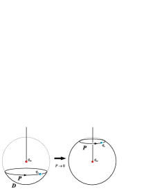
Figure 2.4: We can shrink the path $\mathcal{P}$ to zero around the Dirac String so that the surface $\mathcal{D}$ on the left closed to a two sphere $S^{2}$.

In $D=10$ a similar phenomenon occurs for the extended objects that are sources for the RR p-forms, with the difference that electric and magnetic duals objects generally have a different number of dimensions.

For example we have seen that type IIA contains $C_{1}$, $C_{3}$ and and their respective (fieldstrength) Hodge duals $C_{5}$, $C_{7}$. If $C_{1}$, $C_{3}$ couple electrically with respectively a 0-brane, 2-brane, $C_{7}$, $C_{5}$ couple magnetically to their dual 6-branes, 4-branes. In a regime where the electric coupling is weak, the 6-branes, and 4-branes are thus non-perturbative objects that can wrap some of the compact directions of ten-dimensional spacetime, while invading the extended directions, so that they do not break Poincarè invariance of the uncompactified spacetime.

The presence of p-branes therefore enrich the possibilities for string background, in fact for some configurations, they can preserve some of the supersymmetries of the original theory on the vacuum, moreover these solitons are indeed Dirichlet p-branes (D-p branes) hypersurfaces where closed strings can open up [36], and therefore their quantum excitations can be described by open strings with end-points confined on their world-volumes.

Backgrounds with the presence of D-p branes are of main interest for the present discussion. Together with other objects (orientifold planes), they allow to find consistent solutions for the string equations of motion with an exact world-sheet description, involving closed and open strings. One of the focus in the following will be the study of possible mechanisms for supersymmetry breaking that can be suggested by the presence of D-branes and orientifold planes.

We want to finish this section by analysing the relation between $\mathcal{N}=(1,1)$ superconformal symmetry of the fermionic string Action (2.80) and the extended algebras $\mathcal{N}=(2,2)$ described in a more abstract way in the previous section. We have seen that by choosing a lightcone gauge (2.100) one eliminates the longitudinal oscillators from the dynamical degrees of freedom. If one picks up the superconformal gauge (2.79), the leftover bosonic and fermionic fields represent a system of $2\cdot(D-2)$-free fields. Actually, an Action for their oscillating degrees of freedom enjoies $\mathcal{N}=(2,2)$ superconformal symmetry, as one can check by coupling the coordinates in complex pairs $X^{I}=X^{i}+iX^{i+1}$, $\lambda^{I}=\lambda^{i}+i\lambda^{i+1}$ and $\bar{\lambda}^{I}=\bar{\lambda}^{i}+i\bar{\lambda}^{i+1}$ with $i=1,3,5,7,9$.

The action for the free system of oscillators degrees of freedom then will look like

$$S=\frac{1}{2\pi\alpha^{\prime}}\int dzd\bar{z}\left(\partial X^{I}\bar{\partial}X^{I}+i\lambda^{I}\partial\lambda^{I}+i\bar{\lambda}^{I}\bar{\partial}\bar{\lambda}^{I}\right),$$ (2.125)

where $I=1,2,3,4.$. It is easy then to check that the holomorphic $\mathcal{N}=2$ supercurrents

$$T(z) = -\partial X^{I}\partial X^{I*}+\frac{1}{2}\psi^{I*}\partial\psi^{I}+\frac{1}{2}\psi^{I}\partial\psi^{I*},$$

$$G^{+}(z) = \frac{1}{2}\psi^{I*}\partial X^{I},$$

$$G^{-}(z) = \frac{1}{2}\psi^{I}\partial X^{I*},$$

$$j(z) = \frac{1}{4}\psi^{I*}\psi^{I},$$ (2.126)

satisfy the OPE given in (2.71) and (2.72), that define the $\mathcal{N}=2$ superconformal symmetry.

We have seen in the previous section that for $\mathcal{N}=(2,2)$ superconformal algebra different choices of periodicity conditions for the supercurrents give rise to sets of charges that generate isomorphic algebras. The realisation of this isomorphism, called spectral flow, on the representation of the algebras is obtained by an operator playing on the world-sheet the role of a spacetime supersymmetry charge.

Indeed spacetime supersymmetry is gained after imposing the existence of a square root brunch cut in the OPE between the spectral flow operator and the allowed primary fields of the theory, a condition that translates into a projection on their $U(1)$ charges (generalised GSO projections [31, 32]).

We therefore expect from the critical $D=10$ theory solutions with some ammount of spacetime supersymmetry, by taking sets of fields with different twisted periodicity conditions more general than the Ramond and the Neveu-Schwarz ones. This actually is the case if a correct $U(1)$ projection on the states is performed. The price for introducing these twisted sectors is to break some of the original $SO(1,9)$ spacetime invariance. This is quite natural, if one considers some of the extra-dimensions to be compact, so that the original symmetry breaks to $SO(1,9)\rightarrow SO(1,9-k)\otimes SO(k)$. Since the original $D=10$ flat spacetime type II solutions possess 32 supercharges (the number of components of the two ten-dimensional Majorana-Weyl spinors), a simple toroidal compactification preserving all the supercharge gives rise to a by far too large number of supersymmetries.

Theories with $\mathcal{N}=(2,2)$ allow to introduce different twisted boundary conditions and through a generalised GSO can give rise to a reduced number of supersymmetries in the compactifications. These solutions are called orbifold compactifications [37, 38], a subject on which we will return in chapter five by describing some special examples.

2.4 The torus partition function

As a further step one can consider topologies different then the sphere for the closed (super)string world-sheet. These two dimensional surfaces are called closed Riemann surfaces and are classified by their genus $g$ that corresponds to the number $h$ of handles. The Riemann sphere has $g=h=0$, the torus $g=h=1$ and so on. The Euler characteristic of the surface $\chi$ is a topological invariant

$$\chi=\frac{1}{8\pi}\int\sqrt{g}R^{(2)}=2-2g,$$ (2.127)

with $R^{(2)}$ the scalar curvature of the surface.

The interest of genus $g$ string world-sheets follows from the the Polyakov integral [9, 33]

$$\int\mathcal{D}g_{ab}\mathcal{D}X^{\mu}e^{-S},$$ (2.128)

that allows to compute in a perturbative regime string amplitudes by summing over all the possible topologies of the world-sheet diagrams (fig.2.5).

For a constant dilaton background, the dilaton term of the world-sheet action becomes proportional to the Euler characteristic of the surface

$$\frac{\phi}{8\pi}\int\sqrt{g}R^{(2)}=(2-2g)\phi,$$ (2.129)

and therefore the sum over all the topologies can be expressed as a power expansion in the string coupling constant $g_{s}=e^{-\phi}$

$$\int\mathcal{D}g_{ab}\mathcal{D}X^{\mu}e^{-S}=\sum_{g=0}^{\infty}g_{s}^{2g-2}\int_{\Sigma_{g}}\mathcal{D}g_{ab}\mathcal{D}X^{\mu}e^{-S^{\prime}},$$ (2.130)

$S^{\prime}$ being the world-sheet action without the dilaton term.

For every term in the above sum, the path integral is now performed only on surfaces of fixed genus $g$. If the string coupling is small, eq. (2.130) represents a perturbative expansion that gives a diagrammatic definition for the theory, where Riemann surfaces replace ordinary Feynman diagrams, with a single string diagram for every perturbative order in $g_{s}$.

For every term in the series the integration over the metric involves an integration over the moduli, complex parameters that describe the shape of the surface. The sphere has no moduli, the torus has a complex modulus and a $g\geq 2$ surface has $3(g-1)$ complex moduli.

The moduli are defined on special regions, called fundamental regions $\mathcal{F}_{g}$, of $\mathbb{C}^{n}$ where every point describes an inequivalent shape of the surface. The points outside of the region $\mathbb{C}^{n}-\mathcal{F}_{g}$ are redundant since are connected to those in $\mathcal{F}_{g}$ via modular transformations. Modular transformations form a group $\mathcal{G}_{g}$ called the modular group so that a fundamental region is the quotient $\mathcal{F}_{g}=\mathbb{C}^{n}/\mathcal{G}_{g}$ of the complex plane by the modular group.

An important point is that modular invariance for $g\geq 1$ world-sheets path integrals is an essential requirement for the consistency of the closed string theory, in the $g=1$ torus case modular invariance singles out the consistent closed string spectra.

Higher genus $g>1$ modular invariance is satisfied by the theory once modular invariance on the torus and spin-statistics are satisfied, [40, 39, 41]. In the following of this section we will therefore focus on the torus vacuum amplitude.

Figure 2.5: The perturbative series of vacuum fluctuations for the closed string is ordered by incrising genus.

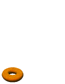
Figure 2.6: The Torus represents the lowest genus topology that gives the lowest order quantum correction to the classical string amplitudes.

The shape of a torus can be described by a complex number $\tau$. This surface can be obtained from a cylinder of height $Im(\tau)$ by gluing together its two boundaries after a relative twist of an amount $Re(\tau)$ (see figure 2.7). We can cut the surface along the two homology cycles of length $Im(\tau)$ and $2\pi$ so that it is represented on a complex plane by a parallelogram with opposite sides identified, fig. 2.8. The torus partition function, that gives the amplitude for a closed string to be created by the vacuum and to describe a fluctuation with a torus world-sheet of shape $\tau$, is given by the following trace on the closed string Hilbert space

$$Z=tr_{\mathscr{H}}e^{-Im(\tau)H+iRe(\tau)P}$$ (2.131)

The Hamiltonian is given by the generator of translations along $\tau$

$$H=2\pi(L_{0}+\bar{L}_{0}),$$ (2.132)

while

$$P=2\pi(L_{0}-\bar{L}_{0})$$ (2.133)

generates translations along $\sigma$.

$e^{-Im(\tau)H}$ realizes a translation equal to the height $Im(\tau)$ of the cylinder, while $e^{iRe(\tau)P}$ gives the $Re(\tau)$ relative twist between the two boundaries and the trace takes care of the gluing between the two boundary of the cylinder so that the initial and final state of the fluctuation are indeed the same.

With the definition $q=e^{2\pi i\tau}$, the partition function can be rewritten as

$$Z=tr_{\mathscr{H}}q^{L_{0}}\bar{q}^{\bar{L}_{0}}.$$ (2.134)

In order to obtain the full vacuum amplitude we need to integrate (2.134) over all the possible shapes $\tau$

$$\mathcal{T}=-\int_{\mathcal{F}}\frac{d^{2}\tau}{\tau_{2}}tr_{\mathscr{H}}\left(q^{L_{0}}\bar{q}^{\bar{L}_{0}}\right).$$ (2.135)

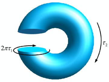
Figure 2.7: A torus can be obtained from a cylinder of height $Im(\tau)$ by gluing together its two boundaries after a relative twist of an amount $2\pi Re(\tau)$

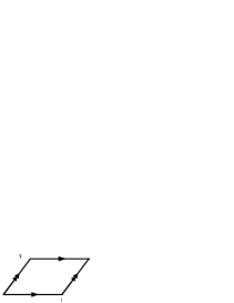
Figure 2.8: By cutting a torus along its two homology cycles, on can be represent this surface on a complex plane by a parallelogram with opposite sides identified.

The integration domain is given by the fundamental region $\mathcal{F}=\{\tau\in\mathbb{C}\ \ |\tau|>1,\ -1/2<\tau_{1}\leq 1/2\}$ of the torus modular group, shown in fig. 2.9. The modular transformations are the big diffeomorphisms on the torus metric that are not connected to the identity, they form a discrete group, whose elements are finite sequences of two basic operations: $T$ and $S$ that leave the shape of the torus unchanged.

$T:\tau\rightarrow\tau+1$ corresponds to add a $2\pi$-twist between the two boundaries of the cylinder before gluing them together, while $S:\tau\rightarrow-1/\tau$ exchanges the two homology cycles of the torus.

The modular group is isomorphic to $PSL(2,\mathbb{Z})$, since a generic sequence of these two basic transformations affects the modular parameter as follows

$$\tau\rightarrow\frac{a\tau+b}{c\tau+d},$$ (2.136)

with $a,b,c,d$ such that $ad-bc=1$.

The integral over the modular parameter $\tau$ that gives the full torus amplitude, needs to be evaluated on the fundamental region $\mathcal{F}=\mathbb{C}/PSL(2,\mathbb{Z})$ of the complex plane, in order not to overcount the contributions from different shapes. The measure $d\tau_{1}d\tau_{2}/\tau_{2}$ that appears in the torus amplitude is not in itself modular invariant , but we will check that the complete final result does.

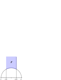
Figure 2.9: Fundamental domain $\mathcal{F}=\mathbb{C}/PSL(2,\mathbb{Z})$ for $\tau$.

We want to compute the torus amplitude for the $D=26$ bosonic string and then for the $D=10$ closed superstring theories.

Let us start with the bosonic string in the light cone gauge. Expressions for $L_{0}$ and $\bar{L}_{0}$ in terms of the transverse oscillators have been given in (2.65), and in the critical dimension read

$$L_{0} = \frac{\alpha^{\prime}}{2}p^{2}+\sum_{m=1}^{\infty}m(a_{m}^{i})^{{\dagger}}a_{m}^{i}-1,$$

$$\bar{L}_{0} = \frac{\alpha^{\prime}}{2}p^{2}+\sum_{m=1}^{\infty}m(\tilde{a}_{m}^{i})^{{\dagger}}\tilde{a}_{m}^{i}-1.$$ (2.137)

A generic closed string state has the form

$$(a_{1}^{i_{1}{\dagger}})^{n_{1}}...(a_{k}^{i_{k}{\dagger}})^{n_{k}}(\tilde{a}_{1}^{j_{1}{\dagger}})^{\tilde{n}_{1}}...(\tilde{a}_{k}^{j_{1}{\dagger}})^{\tilde{n}_{k}}|p,0\rangle$$ (2.138)

with

$$n_{1}+....+n_{k}=\tilde{n}_{1}+....+\tilde{n}_{k}$$ (2.139)

to satisfy the level matching condition, where $n_{i}$ and $\tilde{n}_{i}$ are non negative integers as well as $k$, and $p$ is the spacetime momentum of the centre of mass of the bosonic string.

We first take care of the trace over the continuum of spacetime momenta $p$ in (2.135) that needs to be evaluated over a complete set of momentum eigenstates $\{|p\rangle\}$

$$\mathcal{T} = -\int_{\mathcal{F}}\frac{d^{2}\tau}{\tau_{2}^{2}}Tr_{\mathscr{H}}\left(q^{L_{0}}\bar{q}^{\bar{L}_{0}}\right)$$

$$= -\int\frac{d^{26}p}{(2\pi)^{26}}e^{-\pi\tau_{2}\alpha^{\prime}2p^{2}}\int_{\mathcal{F}}\frac{d^{2}\tau}{\tau_{2}^{2}}Tr\left(q^{\left(\sum m(a_{m}^{i})^{{\dagger}}a_{m}^{i}-1\right)}\bar{q}^{\left(\sum(\tilde{a}_{m}^{i})^{{\dagger}}\tilde{a}_{m}^{i}-1\right)}\right).$$

The Gaussian integral over the momenta then gives

$$\mathcal{T}=-\frac{2^{13}}{(\pi\alpha^{\prime})^{13}}\int_{\mathcal{F}}\frac{d^{2}\tau}{\tau_{2}^{14}}Tr\left(q^{\left(\sum m(a_{m}^{i})^{{\dagger}}a_{m}^{i}-1\right)}\bar{q}^{\left(\sum(\tilde{a}_{m}^{i})^{{\dagger}}\tilde{a}_{m}^{i}-1\right)}\right).$$ (2.140)

The trace over the oscillators yields

$$Tr\left[q^{\left(\sum_{m=1}^{\infty}m(a_{m}^{i})^{{\dagger}}a_{m}^{i}-1\right)}\right]=\prod_{1=2}^{26}Tr\left[q^{\left(\sum_{m=1}^{\infty}m(a_{m})^{{\dagger}}a_{m}-\frac{1}{24}\right)}\right]=q^{-1}\sum_{k=0}^{\infty}d_{k}q^{k},$$ (2.141)

from which one can read the number of closed string states $d_{k}$ that have a mass proportional to $k-1$. In fact the mass shell condition given by $L_{0}|phys\rangle=0$ is

$$m^{2}|phys\rangle=\frac{4}{\alpha^{\prime}}\left(\sum_{m=1}^{\infty}m(a_{m}^{i})^{{\dagger}}a_{m}^{i}-1\right),$$ (2.142)

so that the exponent of $q$ in the l.h.s. of (2.141) is proportional to the masses of the states. The coefficients in front of the various powers of $q$ precisely count the degeneration of every mass level, i.e. the number of closed string states that have a given mass.

Now, in order to obtain the degeneracy coefficients it is enough to think at the structure of the holomorphic sector of the bosonic Fock space. The generic closed string excitation (2.138) has the form $|n_{1}\rangle\otimes....\otimes|n_{k}\rangle\otimes...$ where $n_{i}$ counts the number of bosonic excitation for the mode $i$, whose mass is proportional to $m^{2}\sim n_{1}+2n_{2}+....+kn_{k}+...-1$.

Let us consider first the following set of states of the holomorphic part of the Fock space

$$\mathcal{S}_{1}=\{|i\rangle\otimes|0\rangle....\otimes|0\rangle\otimes...,\qquad i=0,1,2,...\}$$ (2.143)

where the first mode has an arbitrary number $i$ of excitations, while all the other modes are not excited. If we compute the trace of $q^{L_{0}}$ over $\mathcal{S}_{1}$ we obtain:

$$Tr_{\mathcal{S}_{1}}\ q^{\left(\sum_{m=1}^{\infty}m(a_{m})^{{\dagger}}a_{m}-1\right)}=q^{-1}(1+q+q^{2}+....+q^{i}+...)=\frac{q^{-1}}{1-q},$$ (2.144)

while for the subset where only the second mode can be excitated

$$\mathcal{S}_{2}=\{|0\rangle\otimes|j\rangle....\otimes|0\rangle\otimes...,\qquad j=0,1,2,...\}$$ (2.145)

the trace of $q^{L_{0}}$ over $\mathcal{S}_{2}$ gives

$$Tr_{\mathcal{S}_{2}}\ q^{\left(\sum_{m=1}^{\infty}m(a_{m})^{{\dagger}}a_{m}-1\right)}=q^{-1}(1+q^{2\cdot 1}+q^{2\cdot 2}+....+q^{2\cdot i}+...)=\frac{q^{-1}}{1-q^{2}}.$$ (2.146)

If we consider the subset where both the the first two modes are excited but not the others

$$\mathcal{S}_{12}=\{|i\rangle\otimes|j\rangle....\otimes|0\rangle\otimes...,\qquad i,j=0,1,2,...\}$$ (2.147)

the trace of $q^{L_{0}}$ over $\mathcal{S}_{12}$ will be given by the following product

$$Tr_{\mathcal{S}_{12}}\ q^{\left(\sum_{m=1}^{\infty}m(a_{m})^{{\dagger}}a_{m}-1\right)} = q^{-1}(1+q+q^{2}+....+q^{i}+...)\cdot(1+q^{2\cdot 1}+q^{2\cdot 2}+....+q^{2\cdot j}+...)$$ (2.148)

$$= \frac{q^{-1}}{(1-q)(1-q^{2})}$$

because once we compute the product we saturate all the possibilities of exciting independently the first two modes. Therefore the trace over the full holomorphic sector where all the infinite tower of modes can be independently excited is given by the following infinite product

$$Tr\ q^{\left(\sum_{m=1}^{\infty}m(a_{m})^{{\dagger}}a_{m}-1\right)}=\frac{q^{-1}}{(1-q)(1-q^{2})...(1-q^{k})...}=\frac{q^{-1}}{\prod_{n=1}^{\infty}(1-q^{n})}.$$ (2.149)

If one expands the above product up to some order in $q$, $d_{0}+d_{1}q+...+d_{k}q^{k}$, the coefficients $d_{i}$ will correspond to number of states that have a mass equal to the corresponding power of $q$.

Finally, when we compute the trace over the full Fock space of the bosonic string we have to remember that we have 24 identical copies of the Fock space, one for each transverse coordinate, so that

$$Tr\left[q^{\left(\sum_{m=1}^{\infty}m(a_{m}^{i})^{{\dagger}}a_{m}^{i}-1\right)}\right]=\prod_{1=2}^{26}Tr\left[q^{\left(\sum_{m=1}^{\infty}m(a_{m})^{{\dagger}}a_{m}-\frac{1}{24}\right)}\right]$$

$$=\left(\frac{1}{q^{1/24}\prod_{n=1}^{\infty}(1-q^{n})}\right)^{24}=\left(\frac{1}{\eta(q)}\right)^{24},$$ (2.150)

where $\eta(q)$ is the Dedekind eta function.

Altogether the torus amplitude in (2.140) reads

$$\mathcal{T}=-\frac{2^{13}}{(\pi\alpha^{\prime})^{13}}\int_{\mathcal{F}}\frac{d^{2}\tau}{\tau_{2}^{14}}Tr\left(q^{\left(\sum m(a_{m}^{i})^{{\dagger}}a_{m}^{i}-1\right)}\bar{q}^{\left(\sum(\tilde{a}_{m}^{i})^{{\dagger}}\tilde{a}_{m}^{i}-1\right)}\right)$$ (2.151)

$$=-\frac{2^{13}}{(\pi\alpha^{\prime})^{13}}\int_{\mathcal{F}}\frac{d^{2}\tau}{\tau_{2}^{14}}\frac{1}{(\eta(q)\eta(\bar{q}))^{24}}=-\frac{1}{(\pi\alpha^{\prime})^{13}}\int_{\mathcal{F}}\frac{d^{2}\tau}{\tau_{2}^{2}}\frac{1}{\tau_{2}^{12}(\eta(q)\eta(\bar{q}))^{24}}.$$ (2.152)

One can check the modular invariance of the torus vacuum amplitude by using the modular properties of the Dedekind function

$$T:\ \eta(\tau+1)=e^{i\pi/12}\eta(\tau),\qquad S:\ \eta(-1/\tau)=\sqrt{-i\tau}\ \eta(\tau).$$ (2.153)

The measure $d^{2}\tau/\tau_{2}^{2}$ is by itself modular invariant, while for the rest of the integrand function

$$T:\ \ \frac{1}{\tau_{2}^{12}(\eta(\tau+1)\eta(\bar{\tau}+1))^{24}}=\frac{1}{\tau_{2}^{12}(\eta(\tau)\eta(\bar{\tau}))^{24}}$$

$$S:\ \ \frac{|\tau|^{24}}{\tau_{2}^{12}(\eta(-1/\tau)\eta(-1/\bar{\tau}))^{24}}=\frac{1}{\tau_{2}^{12}(\eta(\tau)\eta(\bar{\tau}))^{24}}.$$ (2.154)

thus showing the invariance of the integrand under a generic modular transformation.

The torus partition function corresponds to the torus vacuum amplitude with the omission of the integration in $\tau$ and the normalization coefficient

$$Z=\frac{1}{(\eta(q)\eta(\bar{q}))^{24}}=\frac{1}{q\bar{q}\prod_{n=1}^{\infty}(1-q^{n})^{24}\prod_{n=1}^{\infty}(1-\bar{q}^{n})^{24}},$$ (2.155)

by expanding the infinite products we can read the number of states corresponding to a given mass as the coefficient in front of the powers $(q\bar{q})^{k}$. Since the background for the closed string where we have computed the spectrum is $D=26$ Minkowski spacetime we expect that every string state carry a representation of $SO(1,25)$. In particular since we are working in the light cone gauge we expect to read from the partition function only the physical degrees of freedom, which implies that massless states should carry a representation of $SO(24)$, while massive states should come in representation of $SO(25)$.

Up to massive states the expansion gives

$$Z=\frac{1}{q\bar{q}\prod_{n=1}^{\infty}(1-q^{n})^{24}\prod_{n=1}^{\infty}(1-\bar{q}^{n})^{24}},=(q\bar{q})^{-1}(1+24^{2}q\bar{q}+...)=(q\bar{q})^{-1}+24^{2}(q\bar{q})^{0}+O(q\bar{q})$$ (2.156)

the first term $(q\bar{q})^{-1}$ corresponds to one degree of freedom (its coefficient) i.e. a Lorentz scalar with a negative mass (its exponent). This state is the infamous closed string tachyon. The second term $24^{2}(q\bar{q})^{0}$ indicates $24^{2}=576$ massless degrees of freedom. These are the massless states in the bosonic string spectrum previously described that carry a representation of the massless little group $SO(24)$ of the $D=26$ Lorentz group. The decomposition in irreducible representation gives

$$24^{2}=\left(\frac{24\cdot 25}{2}-1\right)+\left(\frac{24\cdot 23}{2}\right)+(1)=(299)+(276)+(1)$$ (2.157)

the traceless symmetric part $(299)$ of the two tensor corresponds to the physical degrees of freedom of the metric $G_{\mu\nu}$, the antisymmetric part $(276)$ to those of the $B_{\mu\nu}$ and the trace part $(1)$ to the dilaton $\phi$.

Figure 2.10:

Now we turn to consider the $D=10$ closed string theories and compute their torus partition functions. We will compute here the $L_{0}$ traces in the diverse sectors, introduce the notion of characters and show how consistent superstring theories can be obtained by imposing modular invariance. As before, the general form for the torus amplitude is

$$\mathcal{T}=-\int_{\mathcal{F}}\frac{d^{2}\tau}{\tau_{2}}tr_{\mathscr{H}}\left(q^{L_{0}}\bar{q}^{\bar{L}_{0}}\right).$$ (2.158)

Where now we have to consider separately the NS sector, where $L_{0}$ reads

$$L_{0}=\frac{\alpha^{\prime}}{4}p^{2}+\sum_{m=1}^{\infty}m(a^{i}_{m})^{{\dagger}}a^{i}_{m}+\sum_{r=1/2}^{\infty}r(b^{i}_{r})^{{\dagger}}b^{i}_{r}-\frac{1}{2},$$ (2.159)

and the R sector, where

$$L_{0}=\frac{\alpha^{\prime}}{4}p^{2}+\sum_{m=1}^{\infty}(a^{i}_{m})^{{\dagger}}a^{i}_{m}+\sum_{r=1}^{\infty}r(d^{i}_{r})^{{\dagger}}d^{i}_{r}.$$ (2.160)

As for the bosonic string, the trace over the ten-dimensional momentum gives a Gaussian integral,

$$\mathcal{T} = -\int_{\mathcal{F}}\frac{d^{2}\tau}{\tau_{2}}Tr_{\mathscr{H}}\left(q^{L_{0}}\bar{q}^{\bar{L}_{0}}\right)$$ (2.161)

$$= -\int\frac{d^{10}p}{(2\pi)^{10}}e^{-\pi\tau_{2}\alpha^{\prime}p^{2}/2}\int_{\mathcal{F}}\frac{d^{2}\tau}{\tau_{2}}Tr\left(q^{L_{0}}\bar{q}^{\bar{L}_{0}}\right)$$

$$= -\frac{2^{5}}{(\pi\alpha^{\prime})^{5}}\int_{\mathcal{F}}\frac{d^{2}\tau}{\tau_{2}^{6}}Tr\left(q^{L_{0}}\bar{q}^{\bar{L}_{0}}\right),$$

where $L_{0}$ does not contain anymore the momentum $p$.

In calculating the contribution from the world-sheet fermions in the NS sector we need to take into account the Pauli exclusion principle, so that every world-sheet fermionic mode can be excited at most once. For example, the subset $\mathcal{S}_{1}$ of the holomorphic Fock space that we were considering in (2.143) contains in this case only two states

$$\mathcal{S}_{1}=\{|i\rangle\otimes|0\rangle....\otimes|0\rangle\otimes...,\qquad i=0,1\}.$$ (2.162)

The first mode can be excited ($i=1$) or not ($i=0$), while all the other modes are not. The trace of $q^{L_{0}}$ over $\mathcal{S}_{1}$, with $L_{0}$ given by (2.159), then yields

$$Tr_{\mathcal{S}_{1}}\ q^{\left(\sum_{r=1/2}^{\infty}r(b_{r})^{{\dagger}}b_{r}-\frac{1}{2}\right)}=q^{-1/2}(1+q^{1/2}),$$ (2.163)

For the subset

$$\mathcal{S}_{12}=\{|i\rangle\otimes|j\rangle\otimes|0\rangle\otimes...,\qquad i,j=0,1\}$$ (2.164)

that contains four states, since the first two modes can be independently excited but not the others, the trace of $q^{L_{0}}$ gives

$$Tr_{\mathcal{S}_{12}}\ q^{\left(\sum_{r=1/2}^{\infty}r(b_{r})^{{\dagger}}b_{r}-\frac{1}{2}\right)}=q^{-1/2}(1+q^{1/2})(1+q).$$ (2.165)

Iterating, the full trace of $q^{L_{0}}$ in the NS sector reads

$$Tr_{NS}\ q^{L_{0}} = Tr_{NS}\ q^{(\sum_{m=1}^{\infty}m(a^{i}_{m})^{{\dagger}}a^{i}_{m}+\sum_{r=1/2}^{\infty}r(b^{i}_{r})^{{\dagger}}b^{i}_{r}-\frac{1}{2})}$$ (2.166)

$$= q^{-1/2}\prod_{i=2}^{10}Tr\ q^{(\sum_{m=1}^{\infty}m(a_{m})^{{\dagger}}a_{m}+\sum_{r=1/2}^{\infty}r(b_{r})^{{\dagger}}b_{r})}$$

$$= \frac{q^{-1/2}\prod_{n}^{\infty}(1+q^{n-1/2})^{8}}{\prod_{n}^{\infty}(1-q^{n})^{8}}=\frac{1}{\eta^{8}}\left(\frac{\theta_{3}}{\eta}\right)^{4},$$

where we have included also the contributions from the eight transverse bosonic excitations, and in the last equality $\theta_{3}$ is one of the Jacobi theta constants, defined by

$$\theta_{3}=\prod_{n}^{\infty}(1+q^{n-1/2})^{2}(1-q^{n}).$$ (2.167)

In computing the trace in (2.166) we need to give boundary conditions to the spinor fields along the two cycles $\sigma\sim\sigma+2\pi$ and $t\sim t+2\pi$ of the worlsheet torus. In the NS sector these fields are anti-periodic along the $\sigma$-cycle, while a single choice between periodic and anti-periodic boundary conditions along the $t$-cycle is inconsistent with modular invariance. To see this one can consider $t$-antiperiodic NS fermions for definiteness, then (2.166) is invariant under an $S$ modular transformation that exchanges the two cycles, since the fields have the same boundary conditions. A $T$ modular transformation adds a $2\pi$ twist to $Re(\tau)$, the real part of the torus modulus, so that the fields now get a further minus sign in moving along the $t$ cycle and therefore (2.166) is not $T$ invariant. The $T$ transformation of (2.166) is equivalent to the choice of perodic boundary conditons along the $t$-cycle, the alternative choice respect to the one we were considering

$$Tr_{NS}\ q^{L_{0}}\stackrel{{\scriptstyle T}}{{\leftrightarrow}}Tr_{NS}\ (-)^{G}\ q^{L_{0}}$$ (2.168)

where the insertion of the operator $(-)^{G}$ in the trace exchange the fermionic boundary conditions along the $t$-cycle.

An $S$ transformation on the r.h.s in the previous relation interchanges the $\sigma$ with the $t$ cycles, the resulting expression results in a trace computed with $\sigma$-periodic and $t$-antiperiodic boundary conditions, that corresponds to the Ramond sector.

$$Tr_{NS}\ (-)^{G}\ q^{L_{0}}\stackrel{{\scriptstyle S}}{{\leftrightarrow}}Tr_{R}\ q^{L_{0}}.$$ (2.169)

To summarise, a closed modular orbit is given by, (see fig. 2.11)

$$Tr_{NS}\ q^{L_{0}}\stackrel{{\scriptstyle T}}{{\leftrightarrow}}Tr_{NS}\ (-)^{G}\ q^{L_{0}}\stackrel{{\scriptstyle S}}{{\leftrightarrow}}Tr_{R}\ q^{L_{0}},$$ (2.170)

and therefore all the above sectors need to be considered in order to construct modular invariant amplitudes. There is a fourth possibility in prescribing the boundary conditions that we did not considered yet. It corresponds to periodicity along both cycles

$$Tr_{R}\ (-)^{G}\ q^{L_{0}}.$$ (2.171)

This last quantity is modular invariant in itself, therefore it represents a closed modular orbit, disjoint from (2.170).

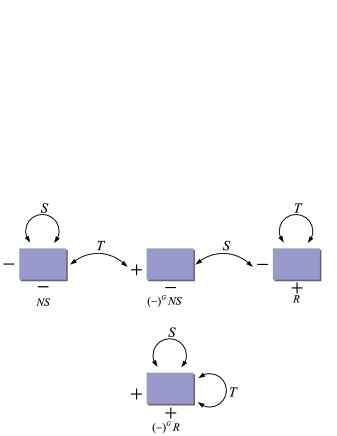
Figure 2.11: The fermionic spin structures on the torus are organised in two disjoint modular orbits. An insertion of the world-sheet holomorphic fermion index $(-)^{G}$ in the trace flips the periodicity conditions along the time direction (vertical side of the torus).

We now compute the trace in the NS sector with the operator $(-)^{G}$ inserted. Notice that $(-)^{G}$ simply gives a minus sign to states with an odd number of $b$ excitations, so that

$$Tr_{NS}\ \left((-)^{G}\ q^{(\sum_{m=1}^{\infty}m(a^{i}_{m})^{{\dagger}}a^{i}_{m}+\sum_{r=1/2}^{\infty}r(b^{i}_{r})^{{\dagger}}b^{i}_{r}-\frac{1}{2})}\right) = \frac{q^{-1/2}\prod_{n}^{\infty}(1-q^{n-1/2})^{8}}{\prod_{n}^{\infty}(1-q^{n})^{8}}$$ (2.172)

$$= \frac{1}{\eta^{8}}\left(\frac{\theta_{4}}{\eta}\right)^{4},$$

where $\theta_{4}$, another Jacobi theta constant, is defined by

$$\theta_{4}=\prod_{n}^{\infty}(1-q^{n-1/2})^{2}(1-q^{n}).$$ (2.173)

With the final goal of obtaining modular invariant torus amplitudes, we are therefore led to consider the following two choices for the NS sector

$$Tr_{NS}\left(\frac{1\pm(-)^{G}}{2}\ q^{L_{0}}\right) = \frac{q^{-1/2}}{\prod_{n}^{\infty}(1-q^{n})^{8}}\left(\frac{\prod_{n}^{\infty}(1+q^{n-1/2})^{8}\pm\prod_{n}^{\infty}(1-q^{n-1/2})^{8}}{2}\right)$$ (2.174)

$$= \frac{1}{\eta^{8}}\frac{\theta_{4}^{4}\pm\theta_{3}^{4}}{2\eta^{4}},$$

which single out the two subsets $NS_{-}$ and $NS_{+}$ of the $NS$ sector.

The lowest state in $NS_{-}$ is a massless vector and all the other states are massive tensors, while the lowest state in $NS_{+}$ is the tachyonic scalar and all the other states are massive tensors. With this in mind, we define the following characters that correspond to the contribution form holomorphic spinor oscillators for the two different GSO projections [48, 60]

$$V_{8} = \frac{\theta_{4}^{4}-\theta_{3}^{4}}{2\eta^{4}},$$

$$O_{8} = \frac{\theta_{4}^{4}+\theta_{3}^{4}}{2\eta^{4}}.$$ (2.175)

Their names recall the lowest mass state that they contain, $V$ for the vector and $O$ for the scalar.

Turning to the R sector, let us start with

$$Tr_{R}\ q^{L_{0}} = Tr_{R}\ q^{(\sum_{m=1}^{\infty}m(a^{i}_{m})^{{\dagger}}a^{i}_{m}+\sum_{r=1}^{\infty}r(d^{i}_{r})^{{\dagger}}d^{i}_{r})}$$ (2.176)

$$= 2^{4}\prod_{i=2}^{10}Tr\ q^{(\sum_{m=1}^{\infty}m(a_{m})^{{\dagger}}a_{m}+\sum_{r=1}^{\infty}r(b_{r})^{{\dagger}}b_{r})}$$

$$= 2^{4}\frac{\prod_{n}^{\infty}(1+q^{n})^{8}}{\prod_{n}^{\infty}(1-q^{n})^{8}}=\frac{1}{\eta^{8}}\left(\frac{\theta_{2}}{\eta}\right)^{4}$$

where one has to take into account that the holomorphic R ground state is a ten dimensional massless spinor, whose physical degrees of freedom correspond to the 16 components of an $SO(8)$ spinor, while the Jacobi $\theta_{2}$ constant is defined by

$$\theta_{2}=2q^{1/8}\prod_{n}^{\infty}(1+q^{n})^{2}(1-q^{n}).$$ (2.177)

We can consider two different GSO projections for the Ramond sector with the insertion of the operator $(-)^{G}\Gamma_{9}$ that selects one of the two chiralities for the spinors.

If one computes the trace over the Ramond sector with the $(-)^{G}\Gamma_{9}$ inserted, one finds

$$Tr_{R}\ \left((-)^{G}\Gamma_{9}q^{L_{0}}\right)=\frac{1}{\eta^{8}}\left(\frac{\theta_{1}}{\eta}\right)^{4}=0.$$ (2.178)

This is due to the equal number of opposite chirality states at every mass level. We define the following characters that correspond to the contribution form holomorphic Ramond fermionic oscillators for the two different spacetime chiralities [48, 60]

$$S_{8} = \frac{\theta_{2}^{4}-\theta_{1}^{4}}{2\eta^{4}},$$

$$C_{8} = \frac{\theta_{2}^{4}+\theta_{1}^{4}}{2\eta^{4}}.$$ (2.179)

So far we have introduced a basis of holomorphic characters that correspond to combinations of the two possible twists along the $\sigma$-cycle (R and NS) and along the $\tau$-cycle ($(-)^{G}$R and $(-)^{G}$NS)

$$O_{8}(q) = tr_{NS}\left(\frac{1+(-)^{G}}{2}\right)q^{L_{0}},\qquad V_{8}(q)=tr_{NS}\left(\frac{1-(-)^{G}}{2}\right)q^{L_{0}},$$

$$C_{8}(q) = tr_{R}\left(\frac{1+\Gamma_{9}(-)^{G}}{2}\right)q^{L_{0}},\qquad S_{8}(q)=tr_{R}\left(\frac{1-\Gamma_{9}(-)^{G}}{2}\right)q^{L_{0}}.$$ (2.180)

These projections, from the spacetime point of view, single out the conjugacy classes for the $SO(8)$ little group. Indeed these classes are the scalar $O$, the vector $V$, and the two spinors $S$, and $C$ with opposite chirality.

The explicit computation of the traces in the above formulae has shown that the SO(8) characters can be written in terms of the four Jacobi theta constants and the Dedekind eta function

$$O_{8} = \frac{\theta^{4}_{3}+\theta^{4}_{4}}{2\eta^{4}},\qquad V_{8}=\frac{\theta^{4}_{3}-\theta^{4}_{4}}{2\eta^{4}}$$

$$C_{8} = \frac{\theta^{4}_{2}+\theta^{4}_{1}}{2\eta^{4}},\qquad S_{8}=\frac{\theta^{4}_{2}-\theta^{4}_{1}}{2\eta^{4}}.$$ (2.181)

From the modular properties of the theta constants it can be derived that a $T$ modular transformation acts on the column vector $(O_{8},V_{8},S_{8},C_{8})$ of (holomorphic) characters with the matrix

$$T=diag(-1,1,1,1),$$ (2.182)

while an $S$ modular transformation acts as

$$\mathcal{S}=\frac{1}{2}\left(\begin{array}[]{cccc}1&1&1&1\\ 1&1&-1&-1\\ 1&-1&1&-1\\ 1&-1&-1&1\end{array}\right).$$ (2.187)

Actually there is a subtlety that one needs to take into account in order to obtain the proper modular transformation properties of the spacetime characters. Due to the opposite statistic, spacetime bosonic and fermionic excitations contribute with an opposite sign to the vacuum energy. This can be taken into account by giving an opposite sign to the holomorphic spacetime fermionic characters $(O_{8},V_{8},-S_{8},-C_{8})$ (and in the anti-holomorphic sector as well). In this case spacetime closed string bosonic and fermionic states that are encoded in products of an holomorphic and one anti-holomorphic characters have opposite sign.

Moreover, we need to ensure that all the interactions respect the GSO projections stated in (2.180) via conditions on the fusion rules coefficients $\mathcal{N}_{hk}^{i}$

$$[f_{h}]\times[f_{k}]=\sum_{hk}\mathcal{N}_{hk}^{i}[f_{i}].$$ (2.188)

Those encode superselection rules coming from the OPEs between fields belonging to different conformal families $[f_{h}]$ and $[f_{k}]$. The fusion rules coefficients $\mathcal{N}_{hk}^{i}$ are connected to the elements of the $S$ modular matrix that acts on the characters via the Verlinde formula [44]

$${N}_{hk}^{i}=\sum_{l}\frac{S_{i}^{l}S_{j}^{l}S_{l}^{k{\dagger}}}{S_{1}^{l}}.$$ (2.189)

It can be proved [45] that a proper account for the spin statistic and the request that all the interactions respect the GSO projections stated in (2.180), interchange the roles of $O_{8}$ and $V_{8}$ in the $S$ and $T$ matrixes. Therefore for the $SO(8)$ spacetime characters $(O_{8},V_{8},-S_{8},-C_{8})$ the correct form for the $S$ matrix is

$$\mathcal{S}=\frac{1}{2}\left(\begin{array}[]{cccc}1&1&-1&-1\\ 1&1&1&1\\ 1&-1&1&-1\\ 1&-1&-1&1\end{array}\right).$$ (2.194)

This is indeed a crucial point to keep in mind in order to recover all the possible ten dimensional closed string modular invariant partition functions.

Knowing the modular properties of the characters we can search for the possible modular invariant sesquilinear combinations of characters. Actually there are four possible choices, the Type IIA and Type IIB combinations [46, 47]

$$Z_{IIA} = (V_{8}-S_{8})(\bar{V}_{8}-\bar{C}_{8})=V_{8}\bar{V}_{8}+S_{8}\bar{C}_{8}-V_{8}\bar{C}_{8}-\bar{V}_{8}S_{8},$$

$$Z_{IIB} = (V_{8}-S_{8})(\bar{V}_{8}-\bar{S}_{8})=V_{8}\bar{V}_{8}+S_{8}\bar{S}_{8}-V_{8}\bar{S}_{8}-\bar{V}_{8}S_{8},$$ (2.195)

and the Type 0A and Type 0B combinations [48]

$$Z_{0A} = O_{8}\bar{O}_{8}+V_{8}\bar{V}_{8}+S_{8}\bar{C}_{8}+C_{8}\bar{S}_{8},$$

$$Z_{0B} = O_{8}\bar{O}_{8}+V_{8}\bar{V}_{8}+S_{8}\bar{S}_{8}+C_{8}\bar{C}_{8}.$$ (2.196)

In the above formulae we have displayed only the contributions from world-sheet fermions excitations. The complete torus amplitudes including also the contributions from the transverse bosonic oscillators and the integration over the torus modular parameter are given by (see 2.161)

$$\mathcal{T}_{IIA}=-\frac{2^{5}}{(\pi\alpha^{\prime})^{5}}\int_{\mathcal{F}}\frac{d^{2}\tau}{\tau_{2}^{6}}\frac{1}{(\eta(q)\eta(\bar{q}))^{8}}(V_{8}-S_{8})(q)(V_{8}-C_{8})(\bar{q})$$

$$=-\frac{2^{5}}{(\pi\alpha^{\prime})^{5}}\int_{\mathcal{F}}\frac{d^{2}\tau}{\tau_{2}^{6}}\frac{1}{4(\eta(q)\eta(\bar{q}))^{12}}(\theta_{3}-\theta_{4}-\theta_{2}+\theta_{1})(q)(\theta_{3}-\theta_{4}-\theta_{2}-\theta_{1})(\bar{q}),$$

and

$$\mathcal{T}_{IIB}=-\frac{2^{5}}{(\pi\alpha^{\prime})^{5}}\int_{\mathcal{F}}\frac{d^{2}\tau}{\tau_{2}^{6}}\frac{1}{(\eta(q)\eta(\bar{q}))^{8}}(V_{8}-S_{8})(q)(V_{8}-S_{8})(\bar{q})$$

$$=-\frac{2^{5}}{(\pi\alpha^{\prime})^{5}}\int_{\mathcal{F}}\frac{d^{2}\tau}{\tau_{2}^{6}}\frac{1}{4(\eta(q)\eta(\bar{q}))^{12}}(\theta_{3}-\theta_{4}-\theta_{2}+\theta_{1})(q)(\theta_{3}-\theta_{4}-\theta_{2}+\theta_{1})(\bar{q})$$

for the supersymmetric closed string theories and similar expression for the type 0 theories. A necessary conditions for supersymmetry on Minkowski space is that at every mass level there is an equal number of bosonic and fermionic degrees of freedom. Since spacetime bosons and fermions contribute with opposite signs in a loop diagram, the supersymmetric vacuum amplitudes $\mathcal{T}_{IIA}$ and $\mathcal{T}_{IIB}$ are expected to vanish. Indeed they vanish as a consequence of the Abstrusa Jacobi Aequatio [49]

$$\theta_{3}^{4}-\theta_{4}^{4}-\theta_{2}^{4}=0,$$ (2.197)

together with $\theta_{1}=0$. Let us extract now the massless spectrum of Type IIA and Type IIB superstrings, by expanding the characters in their corresponding partition functions. Since the excitations of the transverse bosons oscillators are always massive, we use the lighter formulae that involve only contributions from world-sheet spinor oscillators and expand their characters. We start with type IIA, where the holomorphic and anti-holomorphic Ramond sectors have opposite GSO projections

$$Z_{IIA}=(V_{8}-S_{8})(\bar{V}_{8}-\bar{C}_{8})=V_{8}\bar{V}_{8}+S_{8}\bar{C}_{8}-V_{8}\bar{C}_{8}-S_{8}\bar{V}_{8}.$$ (2.198)

We have the bosonic sectors $NS_{-}NS_{-}$ and $R_{-}R_{+}$ encoded in $V_{8}(q)V_{8}(\bar{q})$, and $S_{8}(q)C_{8}(\bar{q})$, and the fermionic sectors $NS_{-}R_{+}$ and $NS_{-}R_{-}$, encoded in $-V_{8}(q)C_{8}(\bar{q})$ and $-S_{8}(q)V_{8}(\bar{q})$.

From the expansion of the $NS_{-}$ character

$$Tr_{NS}\left(\frac{1-(-)^{G}}{2}\ q^{L_{0}}\right) = \frac{q^{-1/2}}{\prod_{n}^{\infty}(1-q^{n})^{8}}\left(\frac{\prod_{n}^{\infty}(1+q^{n-1/2})^{8}\pm\prod_{n}^{\infty}(1-q^{n-1/2})^{8}}{2}\right)$$ (2.199)

$$= \frac{V_{8}}{\eta^{8}}\sim 8q^{0}+O(q)$$

and similarly for the expansions of two Ramond sectors, $R_{-}$

$$Tr_{R}\left(\frac{1-(-)^{G}}{2}\ q^{L_{0}}\right) = \frac{2^{4}}{\prod_{n}^{\infty}(1-q^{n})^{8}}\left(\frac{\prod_{n}^{\infty}(1+q^{n})^{8}}{2}\right)$$ (2.200)

$$= \frac{S_{8}}{\eta^{8}}\hskip 2.84544pt\sim\hskip 2.84544pt8q^{0}+O(q),$$

and $R_{+}$

$$Tr_{R}\left(\frac{1+(-)^{G}}{2}\ q^{L_{0}}\right) = \frac{2^{4}}{\prod_{n}^{\infty}(1-q^{n})^{8}}\left(\frac{\prod_{n}^{\infty}(1+q^{n})^{8}}{2}\right)$$ (2.201)

$$= \frac{C_{8}}{\eta^{8}}\hskip 2.84544pt\sim\hskip 2.84544pt8q^{0}+O(q),$$

we can read the massless spectrum of type IIA.

Indeed in the $NS\otimes NS$ sector

$$V_{8}(q)V_{8}(\bar{q})\sim 64(q\bar{q})^{0}+O(q\bar{q})=(35)+(28)+(1)$$ (2.202)

the $(64)$ massless degrees of freedom correspond to a two-tensor of $SO(8)$, whose irreducible part are the symmetric traceless part $(35)=(8\cdot 9)/2-1$ (spin two ten dimensional graviton $G_{\mu\nu}$), the antisymmetric part $(28)=(8\cdot 7)/2$ that correspond to the excitations of the two form $B_{\mu\nu}$ and the trace $(1)$ excitation of the dilaton $\phi$.

From the $R_{-}R_{+}$ sector we have

$$S_{8}(q)C_{8}(\bar{q})\sim 64(q\bar{q})^{0}+O(q\bar{q})=(8)+(56)$$ (2.203)

the physical degrees of freedom of a one form $C_{1}$ and a tree form $C_{3}$. $(8)$ are the light component of the vector $C_{1}$, while $(56)=(8\cdot 7\cdot 6)/(2\cdot 3)$ are those of $C_{3}$.

$NS_{-}R_{+}$ gives

$$V_{8}(q)C_{8}(\bar{q})\sim 64(q\bar{q})^{0}+O(q\bar{q})=(8_{S})+(56_{C})$$ (2.204)

where we have used the decomposition for the product of the vectorial and (one chirality) spinorial representations $\mathbf{8}_{V}\times\mathbf{8}_{C}=\mathbf{56}_{C}+\mathbf{8}_{S}$ ( the subscripts $C$ and $S$ distinguish the two chiralities). $(56_{C})$ is a left-handed gravitino $\bar{\psi}^{\mu}_{\dot{\alpha}}$ and $(8_{S})$ is a right-handed dilatino $\lambda_{\alpha}$.

While from $R_{-}NS_{+}$

$$S_{8}(q)V_{8}(\bar{q})\sim 64(q\bar{q})^{0}+O(q\bar{q})=(8_{C})+(56_{S})$$ (2.205)

we have $\mathbf{8}_{V}\times\mathbf{8}_{S}=\mathbf{56}_{S}+\mathbf{8}_{C}$, where $(56_{S})$ is a right handed gravitino $\psi^{\mu}_{\alpha}$ and $(8_{C})$ is a left-handed dilatino $\lambda_{\dot{\alpha}}$.

To summarise, for type IIA superstring we have found the following massless spectrum:

bosons:

$$NS_{-}NS_{-} : (G_{\mu\nu},\ B_{\mu\nu},\ \phi)\qquad from\ \ V_{8}(q)V_{8}(\bar{q})$$

$$R_{-}R_{+} : (C_{\mu},\ C_{\mu\nu\rho})\qquad from\ \ S_{8}(q)C_{8}(\bar{q})$$

fermions:

$$NS_{-}R_{+} : (\bar{\psi}^{\mu}_{\dot{\alpha}},\ \lambda_{\alpha})\qquad from\ \ V_{8}(q)C_{8}(\bar{q})$$

$$R_{-}NS_{-} : (\psi^{\mu}_{\alpha},\ \lambda_{\dot{\alpha}})\qquad from\ \ S_{8}(q)V_{8}(\bar{q}).$$

This spectrum corresponds to type IIa $\mathcal{N}=(1,1)$ supergravity that is not chiral.

We now consider the type IIB string, where we employ the same GSO projection in the holomorphic and anti-holomorphic sectors. The partition function thus reads

$$Z_{IIB}=(V_{8}-S_{8})(\bar{V}_{8}-\bar{S}_{8})=V_{8}\bar{V}_{8}+S_{8}\bar{S}_{8}-V_{8}\bar{S}_{8}-S_{8}\bar{V}_{8}.$$ (2.206)

The $NS\otimes NS$ sector is the same as in type IIA case

$$V_{8}(q)V_{8}(\bar{q})\sim 64(q\bar{q})^{0}+O(q\bar{q})=(35)+(28)+(1)$$ (2.207)

and at the massless level comprises $(G_{\mu\nu},\ B_{\mu\nu},\ \phi)$, while the $R_{-}R_{-}$ sector at massless level now containes even-degrees forms

$$S_{8}(q)S_{8}(\bar{q})\sim 64(q\bar{q})^{0}+O(q\bar{q})=(1)+(28)+(35)$$ (2.208)

$(1)$ is a zero form $C_{0}$, $(28)$ a two form $C_{2}$ and $(35)=\frac{1}{2}\frac{8\cdot 7\cdot 6\cdot 5}{2\cdot 3\cdot 4}$ corresponds to the physical degrees of freedom of a four form $C_{4+}$, whose field strength satisfies a self duality conditions

$$\partial_{\mu}C_{\nu\rho\sigma\theta}^{+}=\epsilon_{\mu\nu\rho\sigma\theta}^{\ \ \ \ \ \ \alpha\beta\gamma\delta\eta}\partial_{\alpha}C_{\beta\gamma\delta\eta}^{+}.$$ (2.209)

The RNS spinors from $V_{8}\bar{S}_{8}$ and $S_{8}\bar{V}_{8}$ give two right-handed gravitini and two left-handed dilatini $(\psi^{\mu}_{\alpha},\ \lambda_{\dot{\alpha}})$.

To summarise, the massless spectrum of type IIB superstring is:

bosons:

$$NS_{-}NS_{-} : (G_{\mu\nu},\ B_{\mu\nu},\ \phi)\qquad from\ \ V_{8}(q)V_{8}(\bar{q})$$

$$R_{-}R_{+} : (C,\ C_{\mu\nu},\ C_{\mu\nu\rho\sigma}^{+})\qquad from\ \ S_{8}(q)S_{8}(\bar{q})$$

fermions:

$$NS_{-}R_{-} : (\psi^{\mu}_{\alpha},\ \lambda_{\dot{\alpha}})\qquad from\ \ V_{8}(q)S_{8}(\bar{q})$$

$$R_{-}NS_{-} : (\psi^{\mu}_{\alpha},\ \lambda_{\dot{\alpha}})\qquad from\ \ S_{8}(q)V_{8}(\bar{q}).$$

This spectrum corresponds to type IIb $\mathcal{N}=(2,0)$ supergravity that although chiral is free of anomalies.

————————————————————————————————————–

Chapter 3 $D=10$ Open string Vacua

3.1 Open strings and the Annulus vacuum amplitude

A second option for constructing a quantum theory of a one-dimensional object is to consider the topology of a segment instead of that of a circle. This second possibility gives rise to a description of a quantum open string propagating on spacetime, in many respects related to the closed string theory. At an intuitive level, the relation can be understood by considering that loop open string diagrams, as the one loop annulus for example, represent also closed string tree level diagram (cylinder), see fig. (3.1). Indeed, a theory of open strings needs for its consistency the presence of a closed string sector, while the viceversa is not true. The segment $\{0\leq\sigma\leq\pi\}$ is related to the circle $S=\{\sigma\sim\sigma+2\pi\}$ by one of the simplest examples of orbifold, the quotient $S/\mathbb{Z}_{2}$ with $\mathbb{Z}_{2}:\sigma\rightarrow-\sigma$ as shown in fig (3.3). This already suggests that closed and open string might be at times related in a sort of world-sheet orbifold [50], an idea that we will make precise in the following.

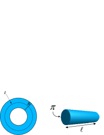
Figure 3.1: The double role of the cylinder as a closed string tree diagram and a one loop open string one. The two possibilities are related by the choice of vertical, along the boundary or horizontal proper time, along the axis.

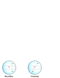
Figure 3.2: The tree-level oriented and unoriented open string diagrams are obtained from two different involutions on a two sphere, (the latter represents a closed string tree-level vacuum diagram). On the left side, the identification of points at opposite latitude gives rise to a disk, whose boundary is the equator. On the right side, the identification of antipodal points on a two sphere produces a semisphere whose equator has opposite points identified (crosscap). The crosscap is isomorphic to the real projective plain.

The involution $\mathbb{Z}_{2}$ creates two boundaries in the infinite cylinder, giving an infinite strip, the world-sheet that the open string describes in its motion. If we introduce complex coordinates $w=\sigma-i\tau$ on the closed string cylinder, so that the world-sheet metric acquires an Euclidean signature, and conformally map this surface into the Riemann sphere $z=e^{iw}=e^{i\sigma}e^{\tau}$, we see that the involution $\mathbb{Z}_{2}:\sigma\rightarrow-\sigma$ translates into $z\sim\bar{z}$, the open string world-sheet becomes the (upper) half complex plane with all the points at infinity identified. This set can also be obtained from the stereographical projection of a disk, whose boundary is projected on the real axis, shown in figure 3.4.

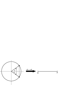
Figure 3.3: The segment $\{0\leq\sigma\leq\pi\}$ is related to the circle $S=\{\sigma\sim\sigma+2\pi\}$ by one of the simplest example of orbifold, the quotient $S/\mathbb{Z}_{2}$ with $\mathbb{Z}_{2}:\sigma\rightarrow-\sigma$. .

All the considerations about the quantisation of the two dimensional world-sheet closed string theory go through for open strings as well, keeping in mind of course that there is only one holomorphic sector and so only one copy of the Virasoro Algebra. This is the result of the boundary conditions on the real axis that impose for the world-sheet fields

$$\partial X^{\mu}(z)=\bar{\partial}X^{\mu}(\bar{z})\qquad on\qquad z=\bar{z},$$ (3.1)

which implies the existence of only one set of oscillators in the open string coordinate mode expansion

$$X^{\mu}(z,\bar{z})=\alpha^{\prime}p^{\mu}\ln|z|^{2}+\sqrt{\frac{\alpha^{\prime}}{2}}\sum_{m\neq 0}\frac{\alpha_{m}^{\mu}}{m}\left(z^{-m}+\bar{z}^{-m}\right).$$ (3.2)

Notice that the open string center of mass momentum is one-half with respect to the closed string case, since the contour integral to obtain it (2.26) needs in this case to be performed over a semicircle.

In particular tree level asymptotic states are created on the boundary of the disk by operators that need to be $SL(2,\mathbb{R})$ invariant. Global scale invariance, in perfect analogy to the holomorphic closed string sector, fixes their conformal weight to be equal to one, so that for the tree level open string spectrum we find the same connections between rank of tensor operators and the masses of the corresponding open string excitations. The open string ground state is necessarily tachyonic, the Lorentz vector is necessarily massless and higher rank tensor states are all necessarily massive.

An important feature, peculiar to open strings, is the possibility of supporting quarks, since their endpoints can be dressed with the so called Chan-Paton factors [51], that give rise to the possibility of describing non-Abelian gauge symmetries. The presence of colours carried by the open string endpoints reflects in the open string amplitudes in the presence of traces of group valued matrices, a feature compatible with the symmetry under cyclic permutation of external legs for these diagrams. A careful investigation of the consistency for the open string amplitudes with unitarity and factorisation at intermediate poles has shown [52, 53] that the allowed open string gauge groups are the classical groups $U(n)$, $SO(n)$ and $USp(2n)$.

We want to focus on open strings in $D=10$ critical dimension, so we consider the $\mathcal{N}=(1,1)$ two dimensional action (2.77) in the superconformal gauge (2.79) on the infinite strip $\mathcal{S}=\{0\leq\sigma\leq\pi,\ -\infty<\tau<\infty\}$

$$S=\frac{1}{4\pi\alpha^{\prime}}\int d\sigma d\tau\partial^{\alpha}X^{\mu}\partial_{\alpha}X_{\mu}+\frac{i}{4\pi\alpha^{\prime}}\int d\sigma d\tau\bar{\psi}^{\mu}\gamma^{\alpha}\partial_{\alpha}\psi_{\mu}.$$ (3.3)

The boundary conditions for the world-sheet fields at the open string endpoints $\sigma=0$ and $\sigma=\pi$ are

$$\delta X^{\mu}\partial_{\sigma}X^{\mu} = 0$$ (3.4)

$$\delta\psi^{\mu}_{L}\psi^{\mu}_{L}+\delta\psi^{\mu}_{R}\psi^{\mu}_{R} = 0\qquad\mu=0,...,D-1,\qquad(not\ summed)$$ (3.5)

where $\psi^{\mu}_{L}$, $\psi^{\mu}_{R}$ are (left)right handed two dimensional spinors. For each of the two endpoint coordinates we can either have $\partial_{\sigma}X^{i}=0$ (Neumann boundary condition) or a $\delta X^{i}=0$ (Dirichlet boundary condition). In the latter case, the endpoint is stuck at one point along the direction given by the coordinate, for example $X^{i}(0,\tau)=x^{i}_{0}$ for the left endpoint or $X^{i}(\pi,\tau)=x^{i}_{\pi}$ for the right one. Open strings can have one or both endpoints constrained to move on a submanifold of the $D=10$ space that is called a Dirichlet p-brane, where $p+1$ is the number of its spacetime dimension. The dimension of a p-brane corresponds to the number of open string coordinates that satisfy Neumann boundary conditions.

For a coordinate that satisfies N-N (Neumann- Neumann) boundary condition the solution of the two dimensional Laplace equation is

$$X^{\mu}=x^{\mu}+\alpha^{\prime}p^{\mu}\tau+\sqrt{\frac{\alpha^{\prime}}{2}}\sum_{n\neq 0}\alpha^{\mu}_{n}e^{in\tau}\cos(n\sigma).$$ (3.6)

In case of mixed N-D (Neumann- Dirichlet) conditions we have instead an expansion in half integer modes

$$X^{\mu}=\sqrt{\frac{\alpha^{\prime}}{2}}\sum_{n}\alpha^{\mu}_{n-1/2}e^{i(n-1/2)\tau}\cos((n-1/2)\sigma),$$ (3.7)

and for D-D (Dirichlet- Dirichlet) boundary conditions

$$X^{\mu}=x^{\mu}\frac{\sigma}{\pi}+\sqrt{\frac{\alpha^{\prime}}{2}}\sum_{n\neq 0}\alpha^{\mu}_{n}e^{in\tau}\sin(n\sigma).$$ (3.8)

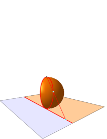
Figure 3.4: Stereographic projection of a disk into the half complex plane, the boundary of the disk is mapped by the projection into the real axis.

Turning to the world-sheet fermions, we have two inequivalent options for satisfying their boundary conditions (3.5)

$$\psi^{\mu}_{L}(0,\tau) = \psi^{\mu}_{R}(0,\tau)$$

$$\psi^{\mu}_{L}(\pi,\tau) = (-)^{a}\psi^{\mu}_{R}(\pi,\tau),$$ (3.9)

where $a=0$ defines the Ramond sector, while $a=1$ the Neveu-Schwarz sector.

By using the basis

$$\psi_{r}=\left(\begin{array}[]{c}\psi_{r,L}\\ \psi_{r,R}\end{array}\right)=\frac{1}{\sqrt{2}}\left(\begin{array}[]{c}e^{-ir(\tau+\sigma)}\\ e^{-ir(\tau-\sigma)}\end{array}\right),$$

of solutions to the two-dimensional Dirac equation, one can write write a generic solution as the expansion

$$\psi=\sum_{r}\left(\beta_{r}\psi_{r,R}+\tilde{\beta}_{r}\psi_{r,L}\right).$$ (3.10)

After imposing the boundary conditions, one finds that $\beta_{r}=\tilde{\beta}_{r}$ and $r\in\mathbb{Z}$ for Ramond, while $r\in\mathbb{Z}+1/2$ for Neveu-Schwarz. Therefore the mode expansions for the two sectors are

$$\psi = \sqrt{\frac{\alpha^{\prime}}{2}}\sum_{r\in\mathbb{Z}}d_{r}\psi_{r},\qquad Ramond,$$

$$\psi = \sqrt{\frac{\alpha^{\prime}}{2}}\sum_{r\in\mathbb{Z}+1/2}b_{r}\psi_{r},\qquad Neveu-Schwarz.$$ (3.11)

Following the same route discussed for one sector of the closed string, one can pick up a light cone gauge and solve the classical constraints for the superconformal algebra for the lightcone oscillators in the various sectors. In this case, longitudinal oscillators are expressed in terms of the physical transverse oscillators and the Hilbert space is manifestly free of negative norm states, because constructed by quantising only transverse modes.

In particular, in order to construct the one-loop open string annulus amplitude we need the generator $L_{0}$ for time translations that in the R sector reads

$$L_{0}=\left(\alpha^{\prime}p^{2}+\sum_{m=1}^{\infty}m(a^{i}_{m})^{{\dagger}}a^{i}_{m}+\sum_{r=1/2}^{\infty}r(b^{i}_{r})^{{\dagger}}b^{i}_{r}-\frac{1}{2}\right),$$ (3.12)

while in the NS sector reads

$$L_{0}=\left(\alpha^{\prime}p^{2}+\sum_{m=1}^{\infty}(a^{i}_{m})^{{\dagger}}a^{i}_{m}+\sum_{r=1}^{\infty}r(d^{i}_{r})^{{\dagger}}d^{i}_{r}\right).$$ (3.13)

Notice the different normalisation of the ten-dimensional momentum $p$ from the closed string case eq. (2.159) and (2.160) as a consequence of (3.2).

The Annulus is a surface that can be obtained from a double covering square torus with a pure imaginary modulus $\tau=i\tau_{2}$ after an anti-holomorphic involution (see fig. 3.5) that creates two boundaries on the covering torus. This amplitude is then given by

$$\mathcal{A} = -N^{2}\int\frac{d\tau_{2}}{\tau_{2}}Tr_{\mathcal{H}}e^{-2\pi\frac{\tau_{2}}{2}L_{0}}$$ (3.14)

$$= -N^{2}\int\frac{d\tau_{2}}{\tau_{2}}Tr_{\mathcal{H}}q^{\frac{1}{2}L_{0}}.$$

The factor $N^{2}$ takes into account the Chan-Paton multiplicities. After computation of the trace over the continuum of the ten dimensional momenta, one recovers

$$\mathcal{A}=-N^{2}\int\frac{d\tau_{2}}{\tau_{2}^{6}}Tr_{\mathcal{H}}q^{\frac{1}{2}L_{0}},$$ (3.15)

where in the last expression to lighten the notation we omitted the normalisation coefficient that originates from the Gaussian integral over the ten dimensional momentum $p$.

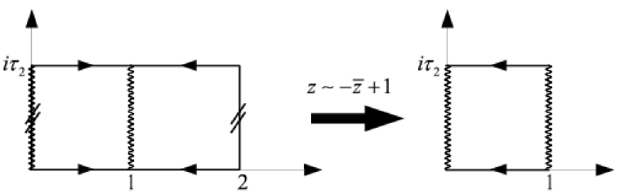
Figure 3.5: The annulus can be obtained from a double covering torus (left side) by the involution $z\sim-\bar{z}+1$ that creates the two boundaries, (represented by the wavy lines). The modulus of the double covering torus $i\tau_{2}/2$, that appears naturally in the Annulus vacuum amplitude (3.17), is obtained by rescaling to one its horizontal side.

Similarly to one sector of the $D=10$ closed string, the ground state in the NS sector is tachyonic, while the first excited state is a massless vector. In the R sector the ground state is instead a ten-dimensional Dirac spinor, while all the excited states are massive.

In order to project out the tachyon and to obtain a supersymmetric open string spectrum, one can consider the various GSO projection on the $SO(8)$ little group characters

$$O_{8}(q) = tr_{NS}\left(\frac{1+(-)^{G}}{2}\right)q^{\frac{1}{2}L_{0}}\qquad V_{8}(q)=tr_{NS}\left(\frac{1-(-)^{G}}{2}\right)q^{\frac{1}{2}L_{0}}$$

$$C_{8}(q) = tr_{R}\left(\frac{1+\Gamma_{9}(-)^{G}}{2}\right)q^{\frac{1}{2}L_{0}}\qquad S_{8}(q)=tr_{R}\left(\frac{1-\Gamma_{9}(-)^{G}}{2}\right)q^{\frac{1}{2}L_{0}}$$ (3.16)

where $(-)^{G}$ is the world-sheet open string fermion number and $q=e^{-2\pi\tau_{2}}$.

For a tachyon-free and spacetime supersymmetric spectrum the right choice in the NS sector is to select the GSO that gives the vector character $V_{8}$, while in the R sector is to select one spinorial character of definite chirality

$$\mathcal{A}=N^{2}\int\frac{d\tau_{2}}{\tau_{2}^{6}\eta^{8}(i\tau_{2}/2)}(V_{8}-S_{8})(i\tau_{2}/2).$$ (3.17)

The opposite sign between the NS and the R characters takes into account that, due to their opposite statistic, bosons and fermions give opposite contributions to the vacuum energy.

The integral in eq. (3.17) needs to be performed on the region $0<\tau_{2}<\infty$ since there is not a modular group for the annulus, in particular there is not an $S$ transformation that cuts off the UV part of the integration domain, and the amplitude is divergent in the UV limit $\tau_{2}\rightarrow 0$.

One can study this divergence from the closed string point of view. In fact, the annulus can be considered as an amplitude for a tree level propagation for closed strings. In order to obtain the correct closed string amplitude, that corresponds to a different choice of proper time, one first makes the change of integration variable $\tau_{2}=2t$

$$\mathcal{A}=N^{2}\int\frac{d\tau_{2}}{\tau_{2}^{6}}Tr_{\mathcal{H}}q^{\frac{1}{2}L_{0}}=2^{-5}N^{2}\int\frac{dt}{t^{6}}Tr_{\mathcal{H}}q^{L_{0}}$$

$$=2^{-5}N^{2}\int\frac{dt}{t^{6}\eta^{8}(it)}(V_{8}-S_{8})(it),$$ (3.18)

in order to obtain the closed string normalisation for the characters, as it appears in the second of the previous equations. ($L_{0}$ does not contain the momentum $p$ as we can see from the power of $t$ in the expression).

Then with the change of variable $t=1/l$ one obtains the correct closed string length in the diagram

$$\tilde{\mathcal{A}}=2^{-5}N^{2}\int_{0}^{\infty}\frac{dl\ l^{4}}{\eta^{8}\left(i/l\right)}(V_{8}-S_{8})\left(i/l\right)=2^{-5}N^{2}\int_{0}^{\infty}\frac{dl}{\eta^{8}(il)}(V_{8}-S_{8})(il).$$ (3.19)

In the last equality we used the transformations properties of the Dedekind eta function under an $S$ transformation $\eta(-1/\tau)=\sqrt{-i\tau}\eta(\tau)$ and the modular invariance of the supercharacter $V_{8}-S_{8}$.

The change of variable $t=1/l$ has mapped the $t\rightarrow 0$ UV divergence into a $l\rightarrow\infty$ IR one.

By expanding the characters in (3.19) in powers of $q=e^{-2\pi l}$ and recalling that the exponents are proportional to the masses of the closed string states flowing in the tube, one can see that the IR divergence of the cylinder is due only to the propagation of massless closed string states

$$\tilde{\mathcal{A}} = 2^{-5}N^{2}\int_{0}^{\infty}\frac{dl}{\eta^{8}(il)}(V_{8}-S_{8})(il)$$ (3.20)

$$= 2^{-5}N^{2}\int_{0}^{\infty}dl\left[(8-8)+(d_{1}-d_{1})e^{-2\pi l}+...+(d_{k}-d_{k})e^{-2\pi lk}+...\right].$$

The origin of the IR divergence is clear by considering that the closed string states flowing on the tube are on-shell

$$\int_{0}^{\infty}dle^{-2\pi lk}=\frac{1}{2\pi k}=\frac{1}{2\pi\alpha^{\prime}p^{2}}\qquad for\ \ p^{2}=m^{2}=\frac{k}{\alpha^{\prime}}.$$ (3.21)

The tree level cylinder amplitude is therefore a sum of on-shell propagators of the $NS\otimes NS$ and RR states flowing in the diagram, multiplied by a coefficient which is the square of the amplitude for emission of the state by a D-p brane (as shown in the upper part in figure 3.11).

These IR divergences are called tadpoles, the $g=1$ cylinder diagram contains tadpole contributions arising from both the $NS\otimes NS$ sector and the RR one, that are indeed $g=1/2$ disk diagrams, as shown in figure 3.6, and that correspond to the emission of massless $NS\otimes NS$ and RR states into the vacuum. They arise in the cylinder diagram in the limit of infinite proper time $l\rightarrow\infty$.

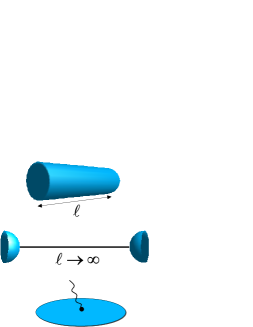
Figure 3.6: Above: The origin of the divergence in the cylinder diagram can be recognised by the factorisation of the amplitude into reflection coefficients at the boundary times on shell propagators. In the limit of infinite closed string proper time $l$ is quite visible the presence of disk tadpole diagrams, that represent the amplitude for emission of closed string from the internal of the disk into the vacuum. These tadpole diagrams gives rise to a divergence for massless states, since the external propagators are forced to be on mass shell.

In the $NS\otimes NS$ sector, the only non-vanishing disk-tadpole diagrams compatible with Lorentz symmetry are those involving the emission of one or more dilatons $\phi$ into the vacuum and the trace $g_{\mu}^{\mu}$ of the graviton. All these diagrams are generated by the following Action term [54]

$$S_{\mathcal{B}}=\mathcal{B}\int d^{10}X\sqrt{G}e^{-\phi},$$ (3.22)

that, after splitting the fields $G_{\mu\nu}=\eta_{\mu\nu}+g_{\mu\nu}$ and $\phi=\phi+\varphi$ into the background plus a fluctuation, computes the amplitude for the emission of $n$ dilatons from the disk

$$\frac{\delta^{n}S_{\mathcal{B}}}{\delta\varphi^{n}}=\frac{1}{n!}\mathcal{B},$$ (3.23)

reproducing the correct combinatory factor $1/n!$ for this diagram, see fig. 3.7.

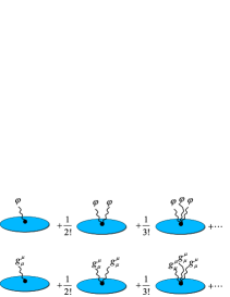
Figure 3.7: The $NS\otimes NS$ tadpole series. Due to Lorentz invariance the only closed string states that can be emitted by a disk are $g^{\mu}_{\mu}$ and $\phi$. The two series can be resummed to obtain the correction term (3.22) for the background fields Action. This corrective term is proportional to the tension of the D-branes present in the background and represents a non vanishing vacuum energy.

The emission for the trace $g_{\mu}^{\mu}$ from the disk can be obtained by expanding the square root $\sqrt{G}=\sqrt{det(\eta_{\mu\nu}+g_{\mu\nu})}=1+g_{\mu}^{\mu}+O(g^{2})$ and by the functional derivarive

$$\frac{\delta}{\delta g_{\mu}^{\mu}}\left(\mathcal{B}\int d^{10}X\sqrt{G}e^{-\phi}\right)=\frac{\delta}{\delta g_{\mu}^{\mu}}\left(\mathcal{B}\int d^{10}Xe^{-\phi}(1+g_{\mu}^{\mu})\right)=\mathcal{B},$$ (3.24)

and similarly for the amplitude for emission of a generic number of states $g_{\mu}^{\mu}$ from the disk.

The action term induced by (3.22) describes a background with a vacuum energy density proportional to $\mathcal{B}$ that is not Ricci flat and therefore seems incompatible with the string equation of motions (2.14), that guarantee conformal invariance on the world-sheet theory. Actually this is not the case, since the tadpole diagram breaks conformal invariance on the world-sheet. An intuitive way to see this is to consider the tadpole diagram, a disk (semisphere) with a tube of infinite length. One way to regularise the divergence is to cut off the length to the tube to a finite size $\bar{l}$. If the insertion of the infinite tube is conformally mapped to a puncture in the interior of the semi-sphere, the presence of a cutoff for its length will correspond to substituting the puncture with a finite size region on the sphere, whose presence breaks conformal invariance since two points on the disk cannot get closer than the size of the region (fig. 3.8).

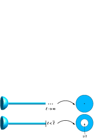
Figure 3.8: One way to regularising the $l\rightarrow\infty$ divergence due to massless modes propagating in the tube is to put a IR cut off $\bar{l}$, that breaks conformal invariance on the disk. A careful inspections shows that conformal symmetry is restored by the cancellation of this effect with the shift on the vacuum energy given by the correction term in eq. (3.22).

The correction of the string equation of motions from the conformal anomaly described above can be connected to the action term describing the tadpole, such that via a redefinition of the background metric from the flat Minkowski to the curved metric satysfing the corrected equations of motions, one obtains conformal invariance again, as first pointed out by Fischler and Susskind [55, 56]. The conformal background, solution of the tadpole corrected string equation of motions, describes a spacetime with a non vanishing Cosmological Constant.

The origin of a nonvanishing vacuum energy is actually connected to the presence of D-branes, whose tension induces a back-reaction on the background generating a curvature. In fact through the cylinder diagram one can measure the tension of a brane, since the $NS\otimes NS$ closed string excanged by two D-branes produces their gravitational interaction and therefore the cylinder diagram is proportional to the square of the tension of a D-brane.

The tension of a D-9 brane, (we are considering open string with Neumann-Neumann boundary conditions on D = 10 spacetime), is proportional to $e^{-\phi}=1/g_{s}$ as one can read from (3.22).

It is worth to mention also that a non vanishing $NS\otimes NS$ tadpole breaks space-time supersymmetry. This happens because supersymmetry guaranties the vanishing of all the tadpoles diagrams. For example, a dilaton tadpole diagram is given by the insertion of a dilaton vertex operator into a point of a Riemann surface. If supersymmetry is present the dilaton vertex operator can be written as the commutator of the supercharge and a fermionic vertex operator. On the world-sheet its local form is given by a contour integral of the above commutator that vanishes for analyticity [27, 28].

The $RR$ tadpole has a rather different meaning since induces a breaking of gauge invariance.

Let us focus on the type IIB. In this case, the only RR form that can propagate in a disk tadpole diagram without breaking ten dimensional Lorentz invariance is the ten form $C_{10}$. This form is not dynamical since its field strength vanishes identically in ten dimensions.

The effective Action term that reproduces the tadpole diagrams for the ten form by functional derivation is

$$S_{C_{10}}=\mathcal{B}_{C_{10}}\int C_{10},$$ (3.25)

which is however incompatible with its equation of motion that states

$$\mathcal{B}_{C_{10}}=0.$$ (3.26)

Therefore an uncancelled RR tadpole from the type IIB brings actually to an inconsistency, since it violates the equation of motion for the RR ten form. A background redefinition that cancels the tadpole in this case does not exist. The inconsistency of an uncancelled RR tadpole manifests itself into an anomaly in the massless spectrum associated to the closed string type IIB excitations and the open string gauge excitations of super Yang Mills. The RR tadpole is associated to the RR charge of the D-9 brane that is measured by the RR contribution to the closed string cylinder diagram. A way to cure this inconsistency is to consider negatively charged extended objects called orientifold planes, whose presence is able to cancel the RR tadpoles and alllow to obtain consistent ten-dimensional vacua, containing a precise number of D9 branes that is called type I superstring.

3.2 Unoriented world-sheets and type I superstring

The involution $\Omega:\sigma\sim-\sigma$ creates two boundaries in the infinite cylinder $\mathbb{R}\times S^{1}$ turning it into the infinite strip $\mathbb{R}\times\left[0,\pi\right]$, the surface that topologically an open string describes in its motion. This involution through the boundaries identifies the holomorphic and antiholomorphic sectors on the world-sheet. However, the involution has been performed only on the classical world-sheet fields and not on the spectrum of their quantum states.

A projection of the open and closed spectra by an operator that realises $\Omega$ on the quantum states will ensure the symmetry at the quantum level, giving rise to an unoriented string theory [48, 81, 85, 57, 58, 59, 60, 61, 62]. It turns out that this projection of the spectrum into unoriented states is the cure for the problems that we have seen in the last section, namely on $D=10$ spacetime the presence of D-9 branes in the background gives rise to an uncancelled RR tadpole which violates the RR ten-form equation of motion. The RR disk tadpole present in the $g=1$ cylinder diagram needs to be cancelled by some other contributions, in order to obtain a consistent string vacuum.

In the unoriented theory there are two more $g=1$ surfaces, besides the torus and the annulus, which are their unorientable cousins the Klein Bottle and the Moebuis strip.

The operator $\Omega:\ \sigma\sim-\sigma$ in the closed string sector interchanges holomorphic and anti-holomorphic oscillators $\Omega:\ \alpha_{-n}^{\mu}\rightarrow\tilde{\alpha}_{-n}^{\mu}$, while in the open sector $\Omega:\ \sigma\sim\pi-\sigma$ acts on the oscillators as $\Omega:\ \alpha_{-n}^{\mu}\rightarrow(-)^{n}\alpha_{-n}^{\mu}$.

As an example, the $NS\otimes NS$ antisymmetric two tensor

$$B_{\mu\nu}:\qquad\left(\alpha^{-1\ \mu}\tilde{\alpha}^{-1\ \nu}-\alpha^{-1\ \nu}\tilde{\alpha}^{-1\ \mu}\right)|0\rangle,$$ (3.27)

is odd under $\Omega$

$$\Omega:B_{\mu\nu}\rightarrow-B_{\mu\nu}.$$ (3.28)

$\Omega$ indeed splits the string spectrum into left-right symmetric states that are even under its action and left-right asymmetric ones that are odd.

If we want $\Omega$ to be a symmetry in the $D=10$ closed superstring spectrum we need to consider type IIB whose right and left moving sectors are identical, (in type IIA the different GSO projections in the R sectors produce only left-right asymmetric states), and project out all the odd states under the $\Omega$ involution.

This can be done by inserting a projector into the trace that computes the closed string one loop vacuum amplitude

$$\int\frac{d^{2}\tau}{\tau_{2}^{6}}Tr\left(\frac{\,\raisebox{1.4pt}{{\hbox{{\rm\scriptsize]}} \raisebox{-1.99997pt}{\kern-8.00003pt\hbox{1}}}}\,+\Omega}{2}\right)q^{L_{0}}\bar{q}^{\bar{L}_{0}}=\frac{1}{2}\mathcal{T}+\mathcal{K}.$$ (3.29)

The number of states in $\mathcal{T}$ have been halved by the projection, while $\mathcal{K}$ is the Klein bottle vacuum diagram whose states complete the projection.

The computation of the trace with the operator $\Omega$ inserted gives

$$\mathcal{K} = \frac{1}{2}\int_{0}^{\infty}\frac{d\tau_{2}}{\tau_{2}^{6}}Tr\left(\Omega q^{L_{0}}\bar{q}^{\bar{L}_{0}}\right)=\frac{1}{2}\int_{0}^{\infty}\frac{d\tau_{2}}{\tau_{2}^{6}}Tr(q\bar{q})^{L_{0}}$$ (3.30)

$$= \frac{1}{2}\int_{0}^{\infty}\frac{d\tau_{2}}{\tau_{2}^{6}\eta^{8}(q\bar{q})}\left(V_{8}-S_{8}\right)(q\bar{q})$$

The trace is not vanishing only on the $NS\otimes NS$ and RR sectors, therefore only states of these sectors flow in the Klein Bottle. The argument of the characters is $q\bar{q}=e^{2\pi i(2i\tau_{2})}$ so that the modulus of the Klein bottle is purely imaginary, and equals $2i\tau_{2}$ .

This has a simple explanation since this unorientable surface can be obtained as an involution from a double covering squared torus with a purely imaginary modulus $2i\tau_{2}$ (see fig. 3.9). After the involution, one recovers the unorientable world-sheet that represents a closed string vacuum fluctuation of proper time $\tau_{2}$. The integral over the Klein Bottle proper time is UV divergent because, as in the case of the open string annulus diagram, there is not any modular symmetry that is able to cutoff the divergence.

One has a second inequivalent choice for the proper time in the Klein bottle, that represents a closed string tree-level tube diagram with two crosscaps (see fig. 3.9). This second choice is connected to the one loop diagram through the change of variable $l=1/2\tau_{2}$ in the integral (3.30), necessary to properly rescale the closed string length.

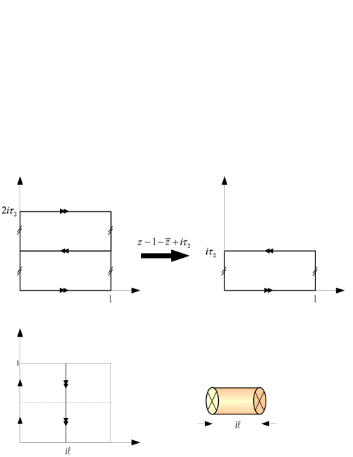
Figure 3.9: Above: the Klein Bottle (on the right side) can be obtained as an involution from a double covering square torus (on the left side) with a pure imaginary modulus $2i\tau_{2}$. This representation corresponds to a choice of vertical proper time. Below: A second inequivalent choice for the proper time for the Klein bottle closed string diagram. The involution from the double covering torus (on the left) shows a representation for this surface as a tube terminating with two crosscaps (on the right). In this second case, we choose horizontal time $l$, and in order to obtain the correct closed string length one needs to impose $l=1/2\tau_{2}$.

The amplitude for tree level closed string propagation between two crosscaps $\tilde{\mathcal{K}}$, corresponding to the choice of horizontal proper time is

$$\tilde{\mathcal{K}}=2^{4}\int_{0}^{\infty}\frac{dl}{\eta^{8}(il)}\left(V_{8}-S_{8}\right)(il).$$ (3.31)

After the change of variable $l=1/2\tau_{2}$, in eq. (3.31) the original UV divergence in the one loop amplitude has been mapped into an IR divergence, due to the massless closed string modes flowing in the tube.

As for the cylinder amplitude, the divergence in the transverse Klein Bottle is due to $NS\otimes NS$ and RR tadpole diagrams, but this time correspond to the emission of massless closed string states from the projective plane into the vacuum.

We now turn to the open string spectrum, where for consistency with the closed sector we need to project the states by $\Omega$. The aim is to check if after having performed a complete projection, both in the closed and in the open sectors, it is possible to find in the $g=1$ amplitudes a cancellation between the disk and the croscap tadpoles.

As for the closed string sector, we project the Fock space of open string excitations by inserting the $\Omega$ projectior into the trace

$$\int_{0}^{\infty}\frac{d\tau_{2}}{\tau_{2}^{6}}Tr\left(\frac{\,\raisebox{1.4pt}{{\hbox{{\rm\scriptsize]}} \raisebox{-1.99997pt}{\kern-8.00003pt\hbox{1}}}}\,+\Omega}{2}\right)q^{L_{0}-1}=\mathcal{A}+\mathcal{M}.$$ (3.32)

Computation of the above expression gives

$$\mathcal{A}=\frac{N^{2}}{2}\int_{0}^{\infty}\frac{d\tau_{2}}{t_{2}^{6}\eta^{8}\left(i\frac{\tau_{2}}{2}\right)}(V_{8}-S_{8})\left(i\frac{\tau_{2}}{2}\right)$$ (3.33)

for the annulus amplitude, while the trace on the open spectrum with $\Omega$ inserted gives the Möbius strip amplitude

$$\mathcal{M} = \int_{0}^{\infty}\frac{d\tau_{2}}{\tau_{2}^{6}}Tr\left(\Omega q^{\frac{1}{2}L_{0}}\right)=\int_{0}^{\infty}\frac{d\tau_{2}}{\tau_{2}^{6}}Tr\left((-q)^{\frac{1}{2}L_{0}}\right)$$ (3.34)

$$= \epsilon\frac{N}{2}\int_{0}^{\infty}\frac{d\tau_{2}}{t_{2}^{6}\hat{\eta}^{8}\left(\frac{1}{2}+i\frac{\tau_{2}}{2}\right)}(\hat{V}_{8}-\hat{S}_{8})\left(\frac{1}{2}+i\frac{\tau_{2}}{2}\right).$$

where $\epsilon$ takes into account for a global sign ambiguity in this amplitude, whose origin will appear clear when we will discuss the corresponding transverse closed string amplitude. The factor $N$ indicates the presence of a single boundary in the surface, (the annulus is proportional to $N^{2}$ due to the two boundaries), while the minus sign in the second equality, that produces an alternating sign in the $q$-expansion of this amplitude, follows from the effect of the reflection $\Omega:\sigma\rightarrow\pi-\sigma$ on the open strings modes

$$\Omega\alpha_{-n}|0\rangle=(-)^{n}\alpha_{-n}|0\rangle.$$ (3.35)

In the last equality of (3.34), we have taken into account the alternating sign $(-)^{n}$ by giving a real part equal to $1/2$ to the pure imaginary argument $i\tau_{2}/2$ in the Möbius characters.

This follows from the definition of the character that is computed on a Verma modulus from a primary state of weight $h$, i.e. the tower of states created by a primary field on the ground state

$$\chi(q)=q^{h-\frac{c}{24}}\sum_{n=0}^{\infty}c_{n}q^{n},$$ (3.36)

with $q=e^{-2\pi\tau_{2}}$ and $c$ the central charge. By adding the real part in the argument of the character it is then necessary to multiply it for a phase in order to recover the original character with the alternating signs

$$q^{h-\frac{c}{24}}\sum_{n=0}^{\infty}(-)^{n}c_{n}q^{n}=e^{-i\pi(h-c/24)}\chi\left(\frac{1}{2}+i\tau_{2}\right)=\hat{\chi}\left(\frac{1}{2}+i\tau_{2}\right).$$ (3.37)

This last relation defines the hatted characters that appear in the loop Möbius amplitude eq. (3.34).

An inequivalent choice for the proper time is possible also for the Möbius strip. This different representation for the world-sheet is given by a tube terminating with a boundary and a crosscap and corresponds to a tree level closed string amplitude.

In this case the double covering surface is not a torus but an annulus with modulus $i\tau_{2}/2$, fig. 3.10. There is a double covering for the Möbius strip as shown in fig. 3.10, but it is a tilted torus with a real part equal to $1/2$ and it is worth noticing that the argument of the characters in the Möbius amplitude correspond to its double covering tilted torus.

The change of integration variable $\tau_{2}=1/t$ in (3.34) is necessary to properly rescale the length of the closed string states flowing in the tube.

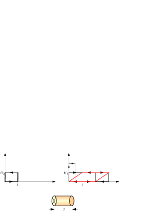
Figure 3.10: On the left above the fundamental polygon for the Möbius strip: following the identifications given by the arrows we can recognise that the wavy lines represent two portions of a single boundary. On the right above, the double covering tilted torus (in red) for the Möbius strip, and the two inequivalent choices for the string proper time. For the horizontal time (below), this surface corresponds to a tube terminating with a boundary and a crosscap.

The transverse tree level amplitude $\tilde{\mathcal{M}}$ therefore reads

$$\tilde{\mathcal{M}}=\epsilon\frac{N}{2}\int_{0}^{\infty}dt\frac{t^{4}}{\hat{\eta}^{8}\left(\frac{1}{2}+\frac{i}{2t}\right)}(\hat{V}_{8}-\hat{S}_{8})\left(\frac{1}{2}+\frac{i}{2t}\right).$$ (3.38)

In order to be able to confront it with $\mathcal{A}$ and $\mathcal{K}$ displaied in (3.19) and (3.31), we need to rewrite this closed string amplitude in terms of characters depending on $1/2+it/2$.

The proper modular transformation that does the job is given by the sequence $P=TST^{2}S$ [48, 81, 85]

$$\frac{1}{2}+\frac{i}{2t}=P\left(\frac{1}{2}+\frac{it}{2}\right).$$ (3.39)

Since in the Möbius amplitude we are using a basis of hatted characters defined in (3.37), the actual representation of the above modular transformation in terms of the matrices $S$ and $T$ is actually slightly modified and is given by $P^{\prime}=T^{1/2}ST^{2}ST^{1/2}$, so that

$$\hat{\chi}_{i}\left(\frac{1}{2}+i\frac{1}{2t}\right)=P^{\prime}_{ij}\hat{\chi}_{j}\left(\frac{1}{2}+i\frac{t}{2}\right),$$ (3.40)

where $T_{ij}^{1/2}=\delta_{ij}e^{i\pi(h-c/24)}$.

By using the $P^{\prime}$ matrix on the hatted characters and the following property for the hatted $\hat{\eta}$ Dedekind function

$$\hat{\eta}\left(\frac{1}{2}+\frac{i}{2t}\right)=\sqrt{t}\ \hat{\eta}\left(\frac{1}{2}+\frac{it}{2}\right),$$ (3.41)

one can re-express the transverse Möbius amplitude (3.42) in terms of modular functions with argument $1/2+it/2$

$$\tilde{\mathcal{M}}=\epsilon\frac{N}{2}\int_{0}^{\infty}\frac{dt}{\hat{\eta}^{8}\left(\frac{1}{2}+\frac{it}{2}\right)}(\hat{V}_{8}-\hat{S}_{8})\left(\frac{1}{2}+\frac{it}{2}\right).$$ (3.42)

Finally, in this amplitude the proper time $t$ needs to be rescaled in order to agree with the proper time of the other two tree amplitudes $\tilde{\mathcal{A}}$ and $\tilde{\mathcal{K}}$, $l=t/2$

$$\tilde{\mathcal{M}}=\epsilon 2\times\frac{N}{2}\int_{0}^{\infty}\frac{dl}{\hat{\eta}^{8}\left(\frac{1}{2}+il\right)}(\hat{V}_{8}-\hat{S}_{8})\left(\frac{1}{2}+il\right).$$ (3.43)

After this rescaling the right factor of 2 appears in front of $\tilde{\mathcal{M}}$ that takes into account the correct combinatory factor for this diagram with respect to $\tilde{\mathcal{A}}$ and $\tilde{\mathcal{K}}$.

The transverse Möbius surface, corresponding to a choice of horizontal proper time, is a tube terminating with a crosscap and a boundary, as it is clear from fig. 3.10. Since the transverse annulus is a tube with two boundaries and the transverse klein bottle a tube with two crosscap, it is then clear that in $\tilde{\mathcal{M}}$ can flow only those closed string states that are common to the other two transerves diagrams, as shown in fig. 3.11. Moreover, the coefficient of the $q=e^{-2\pi l}$ expansion of the amplitude are given by the geometrical mean $\sqrt{\mathcal{B}^{2}\mathcal{C}^{2}}=\pm\mathcal{B}\mathcal{C}$, which is the origin of the overall sign ambiguity taken into account by the sign $\epsilon$.

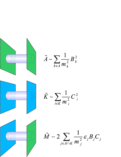
Figure 3.11: The structure of the transverse closed string amplitudes. D-branes are represented in green while O-planes in blue. $\tilde{\mathcal{A}}$ is the amplitude for a closed string two propagate between two D-branes, while $\tilde{\mathcal{K}}$ is the amplitude for propagation between two O-planes. $\tilde{\mathcal{M}}$ describes the amplitude for a closed string to propagate between a D-brane and a O-plane and therefore it contains only the closed string states flowing in both $\tilde{\mathcal{A}}$ and $\tilde{\mathcal{K}}$.

Also in the case of $\tilde{\mathcal{M}}$ the massless states that flow in the diagram generate $NS\otimes NS$ and a RR tadpoles.

We are ready to collect all tadpole contributions from the three diagrams $\tilde{\mathcal{K}}$, $\tilde{\mathcal{A}}$ and $\tilde{\mathcal{M}}$, by considering the constant term in their $q$ expansion, i. e. the coefficients in front of the massless states flowing in the three diagrams. Their total contribution both to the $NSNS$ and to the $RR$ sectors, give (see fig. 3.12)

$$\left(2^{4}+2^{-6}N^{2}+\epsilon N\right)=\frac{1}{64}\left(N+\epsilon 32\right)^{2}.$$ (3.44)

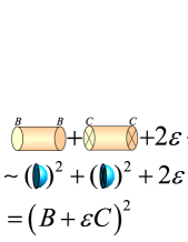
Figure 3.12: Tadpole cancellation is possible among the $g=1$ transverse diagrams $\tilde{\mathcal{K}}$, $\tilde{\mathcal{A}}$ and $\tilde{\mathcal{M}}$, whose divergent part is due to the propagation of closed string massless states. $\tilde{\mathcal{K}}$ is proportional to the square of the crosscap reflection coefficient $\mathcal{C}$, while $\tilde{\mathcal{A}}$ to the square of the boundary reflection coefficient $\mathcal{B}$. $\tilde{\mathcal{M}}$ is proportional to $2\epsilon\mathcal{C}\mathcal{B}$, being the amplitude for closed strings to propagate in a tube diagram terminating with a boundary and a crosscap. The sign ambiguity $\epsilon$ follows by extracting the square root of $(\mathcal{C}\mathcal{B})^{2}$.

Therefore the sum of the $NS\otimes NS$ tadpoles contained in the transverse diagrams induces a correction to the flat background given by

$$\delta S_{\Phi}\sim\left(N+\epsilon 32\right)\int d^{10}xe^{-\Phi}\sqrt{g},$$ (3.45)

while RR tadpoles correct the equation of motion for $C_{10}$ by adding the following term to the Action for the massless modes

$$S_{C_{10}}\sim\left(N+\epsilon 32\right)\int C_{10}.$$ (3.46)

This last contribution cannot be cancelled by a modification of the background fields and leads to an inconsistency unless $\epsilon=-$ and $N=32$, a condition that in this case actually cancels the dilaton tadpole (3.45) as well.

The cancellations of all the tadpoles is necessary for spacetime supersymmetry and indeed one can prove that for $\epsilon=-$ and $N=32$ the full spectrum enjoies $N=1$ spacetime supersymmetry. This background is given by $D=10$ Minkowski with $16$ spacefilling D-9 branes and one O-9 plane. $16$ is actually the number of physical D-9 branes and not $32$ as one might expect. This comes in order to follow a convention consistent with backgrounds with lower dimensional orientifold planes, that we shall discuss in the following. In these cases the lower dimensional planes induce also a reflection symmetry along directions of the target space orthogonal to them which forces to introduce image branes in order to respect this symmetry. In this case the number of physical D-branes is actually one half of the factor $N$ in front of the Möbius.

The configuration of D-9 branes and O-9 planes preserves one-half of the original type IIB supersymmetries, since under world-sheet parity only the sum of holomorphic and anti-holomorphic supercharges survive but not their difference. This solution is called type I superstring whose closed massless spectrum comprises in the closed string $NS\otimes NS$ sector the metric $g_{\mu\nu}$ and the dilaton $\phi$, in the $RR$ sector a two form $C_{2}$ and the (non-dynamical) ten form $C_{10}$.

Finally, the $RNS$ sector yields a gravitino $\Psi_{\alpha}^{\mu}$ and the dilatino $\bar{\zeta}_{\dot{\alpha}}$. The number of physical degrees of freedom in the closed string sectors can be read by expanding the closed string amplitude

$$\frac{1}{2}\mathcal{T}+\mathcal{K} = \frac{V_{8}(q)V_{8}(\bar{q})+V_{8}(q\bar{q})}{2}+\frac{S_{8}(q)S_{8}(\bar{q})-S_{8}(q\bar{q})}{2}-\frac{V_{8}(q)S_{8}(\bar{q})+S_{8}(q)V_{8}(\bar{q})}{2}$$ (3.47)

$$= \frac{8^{2}+8}{2}(q\bar{q})^{0}+\frac{8^{2}+8}{2}(q\bar{q})^{0}-\frac{8^{2}+8}{2}(q\bar{q})^{0}-\frac{8^{2}+8}{2}(q\bar{q})^{0}+O(q\bar{q})$$

In the NSNS sector we have

$$\frac{V_{8}(q)V_{8}(\bar{q})+V_{8}(q\bar{q})}{2}=\left(\frac{8^{2}+8}{2}-1\right)+1+O(q\bar{q})=(35)+(1)+massive$$ (3.48)

the first contribution $(35)$ are the physical degrees of freedom of the graviton $g_{\mu\nu}$, while the second $(1)$ is the dilaton $\phi$.

In the RR sector

$$\frac{S_{8}(q)S_{8}(\bar{q})-S_{8}(q\bar{q})}{2}=\frac{8^{2}-8}{2}=(28)$$ (3.49)

corresponds to the two form $C_{\mu\nu}$.

Finally, the RNS and NSR sectors gives one-half of the degrees of freedom of type IIB

$$\frac{V_{8}(q)S_{8}(\bar{q})+S_{8}(q)V_{8}(\bar{q})}{2}=(64)=\bf{56}_{S}+\bf{8}_{S},$$ (3.50)

which indicates the presence of only one right-handed gravitino $\psi^{\mu}$ and one left-handed dilatino $\bar{\zeta}$, as one can expect from the existence of one spacetime supersymmetry.

Turning to the open string massless spectrum, one can read the physical degrees of freedom from

$$\mathcal{A}+\mathcal{M}=\left(\frac{N^{2}}{2}-\frac{N}{2}\right)V_{8}-\left(\frac{N^{2}}{2}-\frac{N}{2}\right)S_{8}.$$ (3.51)

In the NS open sector we have a massless vector in the adjoint of $SO(32)$, while in the R sector we have the gaugino. The massless open string excitations correspond then to $N=(1,0)$ $SO(32)$ pure super Yang Mills that comprises the vector gauge boson $A_{\mu}^{a}$ and the gaugino $\lambda_{\alpha}^{a}$. The full massless spectrum $(g_{\mu\nu},\phi,C_{\mu\nu},\psi^{\mu},\bar{\zeta},A_{\mu}^{a},\lambda_{\alpha}^{a})$ corresponds to type I supergravity plus super Yang-Mills in $D=10$, which is free of gravitational, gauge and mixed anomalies for the gauge group $SO(32)$.

Due to the sign ambiguity in front of states flowing in the transverse Möbius amplitude one can consider a different solution by relaxing the NSNS tadpole. This corresponds to a different choice of sign for the NSNS and RR states flowing in the Möbius $\epsilon_{NS}=+$, $\epsilon_{R}=-$.

In this case the background is not supersymmetric due to the uncancelled NSNS tadpole and the gauge group becomes $USp(32)$ [63]. The NSNS tadpole generates the dilaton potential

$$V=\left(N+32\right)\int d^{10}x\ \sqrt{g}e^{-\langle\phi\rangle},$$ (3.52)

with a runaway behaviour in the dilaton VEV $\langle\phi\rangle$.

————————————————————————————————————–

Chapter 4 Compactification and Supersymmetric Open String Vacua

One of the main tests for string theory is to check whether on one of its vacua it provides excitations that agree with the standard model of particle physics. If future generation high-energy accelerators will supply evidences for the existence of the superpartners, this would represent an important indirect indication in favour of superstring theory.

One of the main problems is vacuum degeneracy. In the compactification scheme that we are going to discuss the classical spacetime on which the string propagates is the product of four dimensional Minkowski and a compact space. The classical spacetime needs to satisfy the string equations of motion but besides that, a dynamical mechanism that produce the background is not known. In this state of affairs, the vacuum is chosen a priori by hand, and this choice is among an incredible huge spectrum of possibilities. Some of the vacua resemble the properties and the spectrum of the standard model, while other have completely different features. The Standard Model parameters can be in principle reproduced by stabilising string moduli, VEVs of background scalar fields, that describe the compactification. The stabilisation can be achieved, as recent and present investigations have been showing, by intricate combinations of various backgrounds (fluxes) predicted by the superstring. In this way the problem of explaining the SM parameters is translated into the problem of explaining why the fluxes have the values that reproduce correctly the SM parameters. This is another face of the vacuum degeneracy problem.

To find vacua that have features identical to the Standard Model is still an open problem and the precise structure of the low energy particle world poses several constraints and non trivial tasks that at least one of the string solutions need to satisfy.

One of the first criteria that one can follow is to study vacua that preserve some supersymmetries, since the absence of quantum effects on the background allow a good analytic control. Even if the background preserves supersymmetry the choice is still among an amazing huge number of possibilities.

In general a spontaneous breaking of all the supersymmetries lifts the moduli by creating a quantum potential, and the effects of the quantum fluctuations induce on the background are not under control. The background acquires a dynamics such that the initial assumptions are no longer true and one should be able to have an approximation scheme to describe quantum gravity without spacetime supersymmetry and then, probably without the assumption of splitting the spacetime into an inert flat background and quantum fluctuations.

The understanding of some nonperturbative properties of string theory has enlarged the spectrum of the possibilities for the structure of string vacua. Particularly interesting are the D-p branes that are solitons of the theory, a sort of multidimensional generalisation of magnetic monopoles. They are spacetime defects on which closed strings can open up and, quite interestingly they have perturbative excitations that are open strings, so they can be thought of as backgrounds, whose configurations can preserve some amount of the original supersymmetries of the empty spacetime solutions.

In models of brane-worlds the branes invade the four extended dimensions, as represented in fig. 4.1, and wrap some cycles of the compact space.

Figure 4.1:

The standard model forces are mediated by open strings confined on the brane while only gravity, mediated by closed strings, can experience all the ten spacetime dimensions. This has given new possibilies for explaining the observed hierarchy between the electro-weak and the gravitational forces. Gravity is so weak because of the dispersion of its flux lines in a higher number of dimensions comparing to the other forces.

As recent observations have confirmed, the Cosmological Constant is slightly positive so that, at least in the part of universe we live in, the extended space is a de Sitter spacetime with a positive curvature.

4.1 Compactifications

Since in general consistent string models require the presence of extra-dimensions and, in particular, in its perturbative formulation, critical superstrings predict ten space-time dimensions, string vacua that claim to describe low energy physics need to contain compact dimensions. Due to the perturbative stability of the ten dimensional supersymmetric vacua, it seems necessary to consider mechanisms that induce a compactification and, in connection with that, the breakdown of the original $D=10$ supersymmetry .

Let us for the moment put aside the question of finding mechanisms that induce compactification of some of the extra dimensions, such as those induced by the breaking of supersymmetry, and describe the propagation of strings on a priori compactified backgrounds. This becomes easier if some of the original ten-dimensional spacetime supersymmetries are preserved in the compactified solution and it is therefore worth to begin with such situation.

The simplest ansatz for compactification is to consider backgrounds of the form $\mathcal{M}_{d}\otimes\mathcal{X}_{10-d}$, tensor product of a $d$-dimensional Minkowski space with a $(10-d)$-dimensional compact space. Such solutions are generically named compactifications to $d$ dimensions. For this class of vacua one can consider the breaking $SO(1,9)\rightarrow SO(1,d-1)\times SO(10-d)$ of the original ten-dimensional Lorentz symmetry and a consequent Kaluza Klein reduction of the fields that describe string excitations.

With the above breaking of the Lorentz group, the range for the indexes of a tensor field pointing to compact directions counts the number of copies of $SO(1,d-1)$ fields present in the spectrum. This dimensional reduction is actually encoded by the breaking of the original ten dimensional spacetime characters into sum of products of lower dimensional spacetime and internal ones, that at massless level reproduce the expected group theoretical decomposition for the Lorentz irreducible representations. For a compactification to $2d+2$ extended dimensions $SO(1,9)\rightarrow SO(1,2d+1)\times SO(2k)$ with $2d+2+2k=10$, we have the following decomposition

$$O_{8} = O_{2d}O_{2k}+V_{2d}V_{2k},\qquad V_{8}=V_{2d}O_{2k}+O_{2d}V_{2k},$$

$$S_{8} = S_{2d}C_{2k}+C_{2d}S_{2k},\qquad C_{8}=S_{2d}S_{2k}+C_{2d}C_{2k}.$$ (4.1)

The left factors in the above relation indicate spacetime characters, while the right factors are internal characters.

As usual, the lower-dimensional characters are expressed in terms of combinations of Jacobi Theta Constants

$$O_{2n} = \frac{\theta^{n}_{3}(0|\tau)+\theta^{n}_{4}(0|\tau)}{2\eta^{n}},\qquad V_{2n}=\frac{\theta^{n}_{3}(0|\tau)-\theta^{n}_{4}(0|\tau)}{2\eta^{4}},$$

$$C_{2n} = \frac{\theta^{n}_{2}(0|\tau)+i^{-n}\theta^{n}_{1}(0|\tau)}{2\eta^{4}},\qquad S_{2n}=\frac{\theta^{n}_{2}(0|\tau)-i^{-n}\theta^{n}_{1}(0|\tau)}{2\eta^{4}}.$$ (4.2)

One can verify that at every mass level the decompositions (4.1) hold, by using the representations of the Jacobi functions as infinite products given in eqs. (2.167), (2.173), (2.177) and (2.178).

It is worth to notice that the modular properties of the internal characters $(O_{2n},V_{2n},S_{2n},C_{2n})$ follow from those of the Theta functions, and are given by the following matrices

$$T=e^{-i\pi/12}diag\left(1,-1,e^{in\pi/4},e^{in\pi/4}\right),$$ (4.3)

and

$$\mathcal{S}_{2n}=\frac{1}{2}\left(\begin{array}[]{cccc}1&1&1&1\\ 1&1&-1&-1\\ 1&-1&i^{-n}&-i^{-n}\\ 1&-1&-i^{-n}&i^{-n}\end{array}\right).$$ (4.8)

While for spacetime characters $(O_{2n},V_{2n},-S_{2n},-C_{2n})$, for a proper account of spin-statistic, the correct matrices that realise the modular transformations are obtained by interchanging the role of the vector $V_{2n}$ and the scalar $O_{2n}$, as already discussed in section 2.4 for the special case of the $SO(8)$ ten-dimensional characters. One has

$$T=e^{-i\pi/12}diag\left(-1,1,e^{in\pi/4},e^{in\pi/4}\right),$$ (4.9)

$$\mathcal{S}_{2n}=\frac{1}{2}\left(\begin{array}[]{cccc}1&1&-1&-1\\ 1&1&1&1\\ 1&-1&i^{-n}&-i^{-n}\\ 1&-1&-i^{-n}&i^{-n}\end{array}\right).$$ (4.14)

Compactification implies also a Kaluza-Klein reduction for the various fields in the spectrum. By Fourier expanding a given field, periodic along the compact directions, one obtains from the lower dimensional point of view a massless field plus an infinite tower of massive ones.

As an example, after a circle compactification $\mathcal{M}_{9}\times S^{1}$ a scalar field $\phi$

$$\phi(\mathbf{x},y)=\sum_{m\in\mathbb{Z}}\phi_{m}(\mathbf{x})e^{2\pi iym/L},$$ (4.15)

gives rise to a tower of modes $\phi_{m}(\mathbf{x})$

$$\Box\phi_{m}(\mathbf{x})e^{2\pi im/L}=(\Box_{\mathbf{x}}+\partial_{y}^{2})\phi_{m}(\mathbf{x})e^{2\pi im/L}=\left(\Box_{\mathbf{x}}-\left(2\pi m/L\right)^{2}\right)\phi_{m}(\mathbf{x})e^{2\pi im/L},$$ (4.16)

with masses given by

$$M^{2}_{m}=\left(\frac{m}{R}\right)^{2}\qquad m\in\mathbb{Z},$$ (4.17)

$R=L/2\pi$ being the radius of $S^{1}$.

A further tower of massive modes are given by topological non-trivial string configurations in which a closed string winds around a compact direction [64, 65]. Or, for open strings, if two D-branes have a different position on the circle such that the string can stretch between them, partially or completely winding the circle.

In both cases the mass of the topologically non trivial modes is proportional to an integer number, the winding string number and the effective length of the string.

The zero mode part of the closed string coordinate expansion along the circle direction is then given by

$$X_{zm}=x+2\alpha^{\prime}\frac{m}{R}\tau+2nR\sigma\qquad m,n\in\mathbb{Z},$$ (4.18)

where we have changed in the closed string expansion the normalisation in front of the momentum with respect to eq. (2.28) and we have halved the closed string length for convenience in later formulae. To take into account for the change of normalisation it is enough to replace $\alpha^{\prime}\rightarrow 4\alpha^{\prime}$ in all the previous formulae. The corresponding right and left moving zero-mode expansions are

$$X_{zm}(\tau-\sigma) = \frac{x}{2}+\alpha^{\prime}\left(\frac{m}{R}-\frac{nR}{\alpha^{\prime}}\right)(\tau-\sigma)=\frac{x}{2}+\alpha^{\prime}p_{R}(\tau-\sigma),$$

$$X_{zm}(\tau+\sigma) = \frac{x}{2}+\alpha^{\prime}\left(\frac{m}{R}+\frac{nR}{\alpha^{\prime}}\right)(\tau+\sigma)=\frac{x}{2}+\alpha^{\prime}p_{L}(\tau+\sigma),$$ (4.19)

with right and left moving momenta

$$p_{R}=\frac{m}{R}-\frac{nR}{\alpha^{\prime}}\qquad p_{L}=\frac{m}{R}+\frac{nR}{\alpha^{\prime}}.$$ (4.20)

The zero modes therefore give the following contribution to the closed string mass formula

$$M^{2}=\frac{1}{2}(p_{R}^{2}+p_{L}^{2})=\frac{m^{2}}{R^{2}}+\frac{(nR)^{2}}{(\alpha^{\prime})^{2}}.$$ (4.21)

It is then clear the invariance of the closed string spectrum under the T-duality transformation $R\rightarrow\alpha^{\prime}/R$, a symmetry of the full closed string theory [65] that corresponds to the interchange $\sigma\leftrightarrow\tau$ between the two world-sheet coordinates. Its effect on the bosonic coordinates corresponds to the asymmetric transformation $X_{L}^{\mu}\rightarrow X_{L}^{\mu}$, $X_{R}^{\mu}\rightarrow-X_{R}^{\mu}$, which leaves the components of the stress tensor invariant. This same operation induces a reflection on the right-mover world-sheet fermions, thus changing the chirality of the spacetime fermionic states in the holomorphic Ramond sector. Therefore a T-duality exchanges type IIA and type IIB in nine dimensions. However, in the case of circle compactification and for the more general case of higher-dimensional tori, the spacetime spinors get decomposed into lower dimensional spinors of both chiralities and therefore type IIA and type IIB after compactification give rise to the same spectrum.

In the presence of D-branes, a T-duality along a direction exchanges Neumann and Dirichlet boundary conditions [66, 67, 68], thus increasing or decreasing by one the dimensionality of a Dp-brane [69], whether the T-dualised coordinate is orthogonal or parallel to it. The same phenomenon of dimensional transmutation occurs also for orientifold planes, whose action on the spectrum of string states is turned by a T-duality, into a combination of world-sheet parity $\Omega$ and spacetime reflection $I:X\rightarrow-X$ along the T-dualised direction $X$

$$\Omega\stackrel{{\scriptstyle T}}{{\rightarrow}}I\Omega.$$ (4.22)

4.2 Circle Compactifications

We now turn to study some properties of closed string theory after compactification, by computing the torus amplitude for type IIB on the circle $S^{1}$.

The general form for the torus amplitude eq.(2.4) is given by

$$\mathcal{T}=\int_{\mathcal{F}}\frac{d^{2}\tau}{\tau_{2}}Tr_{\mathscr{H}}\left(q^{\frac{1}{4}L_{0}}\bar{q}^{\frac{1}{4}\bar{L}_{0}}\right),\\$$

but in this case along the compact coordinate the momenta $p_{R}$ and $p_{L}$ are quantised.

Therefore performing the trace over the ten dimensional momentum $p$

$$q^{\frac{1}{4}L_{0}}\bar{q}^{\frac{1}{4}\bar{L}_{0}}=e^{-\pi\tau_{2}\frac{1}{2}(L_{0}+\bar{L}_{0})}e^{i\pi\tau_{1}\frac{1}{2}(L_{0}-\bar{L}_{0})},$$ (4.23)

$$e^{-\frac{\pi\tau_{2}\alpha^{\prime}}{2}(p^{2}_{L}+p^{2}_{R})}e^{\frac{i\pi\tau_{1}\alpha^{\prime}}{2}(p^{2}_{L}-p^{2}_{R})}=e^{-\pi\tau_{2}\alpha^{\prime}\left(\frac{m^{2}}{R^{2}}+\frac{(nR)^{2}}{(\alpha^{\prime})^{2}}\right)}e^{2i\pi\tau_{1}mn},$$ (4.24)

one needs to replace the Gaussian integral for the compact direction with a discrete sum over the Kaluza-Klein $m$ and winding $n$ quantum numbers

$$\int\frac{dp}{2\pi}e^{-\pi\tau_{2}\alpha^{\prime}p^{2}}\rightarrow\sum_{m\in\mathbb{Z}}\sum_{n\in\mathbb{Z}}e^{-\pi\tau_{2}\alpha^{\prime}\left(\frac{m^{2}}{R^{2}}+\frac{(nR)^{2}}{(\alpha^{\prime})^{2}}\right)}e^{2i\pi\tau_{1}mn}.$$ (4.25)

The torus amplitude therefore reads

$$\mathcal{T} = \int_{\mathcal{F}}\frac{d^{2}\tau}{\tau_{2}^{6}(\eta\bar{\eta})^{8}}|V_{8}-S_{8}|^{2}\ \cdot\sqrt{\tau_{2}}\sum_{m\in\mathbb{Z}}\sum_{n\in\mathbb{Z}}e^{-\pi\tau_{2}\alpha^{\prime}\left(\frac{m^{2}}{R^{2}}+\frac{(nR)^{2}}{(\alpha^{\prime})^{2}}\right)}e^{2i\pi\tau_{1}mn}$$ (4.26)

$$= \int_{\mathcal{F}}\frac{d^{2}\tau}{\tau_{2}^{6}(\eta\bar{\eta})^{8}}|V_{8}-S_{8}|^{2}\cdot\sqrt{\tau_{2}}\sum_{m,n}\Lambda_{m,n},$$

where

$$\sum_{m,n}\Lambda_{m,n}=\sum_{m,n\in\mathbb{Z}}e^{-\pi\tau_{2}\alpha^{\prime}\left(\frac{m^{2}}{R^{2}}+\frac{(nR)^{2}}{(\alpha^{\prime})^{2}}\right)}e^{2i\pi\tau_{1}mn},$$ (4.27)

indicates a double lattice sum.

To check modular invariance, it is easy to see that $T:\tau_{1}\rightarrow\tau_{1}+1$ leaves the above lattice sum invariant, while to check invariance under $S:\tau\rightarrow-1/\tau$ one needs to use the Poisson resummation formula

$$\sum_{m\in\mathbb{Z}}e^{-\pi m^{2}a+2\pi ib}=\frac{1}{\sqrt{|a|}}\sum_{\mu\in\mathbb{Z}}e^{-\pi a^{-1}(\mu+b)^{2}}.$$ (4.28)

For example a resummation on $m$ gives

$$\sum_{m,n}\Lambda_{m,n}=\frac{R}{\sqrt{\alpha^{\prime}\tau_{2}}}\sum_{\mu,n}e^{-\frac{\pi R^{2}}{\alpha^{\prime}\tau_{2}}|n\tau+\mu|^{2}}.$$ (4.29)

A generic modular transformation in $PSL(2,\mathbb{Z})$, represented by the integral matrix

$$M_{n,\mu}=\left(\begin{array}[]{cc}a&b\\ n&\mu\end{array}\right),$$ (4.32)

transforms the torus parameter as

$$\tau\rightarrow\frac{a\tau+b}{n\tau+\mu},$$ (4.33)

and thus the imaginary part $\tau_{2}$ transforms as

$$\tau_{2}\stackrel{{\scriptstyle M_{n,\mu}}}{{\longrightarrow}}\frac{\tau_{2}}{|n\tau+\mu|^{2}}.$$ (4.34)

We can then rewrite the lattice sum (4.29) as

$$\sum_{m,n}\Lambda_{m,n}=\frac{R}{\sqrt{\alpha^{\prime}\tau_{2}}}\sum_{\mu,n}e^{-\frac{\pi R^{2}}{\alpha^{\prime}\tau_{2}}|n\tau+\mu|^{2}}=\frac{R}{\sqrt{\alpha^{\prime}\tau_{2}}}\sum_{M_{n,\mu}}e^{-\frac{\pi R^{2}}{\alpha^{\prime}M_{n,\mu}\cdot\tau_{2}}},$$ (4.35)

so that the torus amplitude (4.26) becomes

$$\mathcal{T}=\frac{R}{\sqrt{\alpha^{\prime}}}\int_{\mathcal{F}}\frac{d\tau^{2}}{\tau_{2}^{6}(\eta\bar{\eta})^{8}}|V_{8}-S_{8}|^{2}\ \cdot\sum_{M_{n,\mu}}e^{-\frac{\pi R^{2}}{\alpha^{\prime}M_{n,\mu}\tau_{2}}}.$$ (4.36)

From the previous equation it becomes quite visible the modular invariance of the integrand, since it contains the image $M_{n,\mu}\tau_{2}$ of the imaginary part of the torus modulus under the full modular group.

Moreover, one can use the fact that the above amplitude contains a sum over the terms $M_{n,\mu}\tau_{2}$ to unfold the integration domain from the fundamental region $\mathcal{F}$ to the half-strip $\mathcal{S}=\left[-1/2,1/2\right]\times[0,\infty)$. This last region is the image of the fundamental domain through the modular group, modulo unitary translation on the real axis, i.e. [70]

$$\mathcal{S}=PSL(2,\mathbb{Z})(\mathcal{F})/T.$$ (4.37)

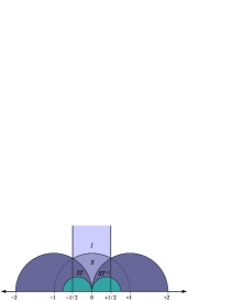
Figure 4.2:

$$\mathcal{T} = \frac{R}{\sqrt{\alpha^{\prime}}}\int_{\mathcal{F}}\frac{d\tau^{2}}{\tau_{2}^{6}(\eta\bar{\eta})^{8}}|V_{8}-S_{8}|^{2}\ \cdot\sum_{M_{n,\mu}}e^{-\frac{\pi R^{2}}{\alpha^{\prime}M_{n,\mu}\tau_{2}}}$$ (4.38)

$$= \frac{R}{\sqrt{\alpha^{\prime}}}\int_{\cup M_{n,\mu}(\mathcal{F})}\frac{d\tau^{2}}{\tau_{2}^{6}(\eta\bar{\eta})^{8}}|V_{8}-S_{8}|^{2}\ \cdot e^{-\frac{\pi R^{2}}{\alpha^{\prime}\tau_{2}}}$$

$$= \frac{R}{\sqrt{\alpha^{\prime}}}\int_{-1/2}^{1/2}d\tau_{1}\int_{0}^{\infty}\frac{d\tau_{2}}{\tau_{2}^{6}(\eta\bar{\eta})^{8}}|V_{8}-S_{8}|^{2}\ \cdot e^{-\frac{\pi R^{2}}{\alpha^{\prime}\tau_{2}}}.$$

In this way we have reduced the integration domain for the torus amplitude into a simpler one, which allows a direct computation of the integral. Of course, for this supersymmetric case this reduction is not of big interest since the integrand is itself vanishing as a result of Jacobi Abstrusa Identity. However we will come back in the following to this unfolding technique[71, 43, 72, 73, 74] for non-supersymmetric vacua where it gives a way to compute one-loop torus potentials.

This last expression shows in particular the presence of an exponential factor that acts as a regulator by cutting off the UV closed string modes in the region $\tau_{2}<\pi R^{2}/\alpha^{\prime}$.

4.3 Rational Conformal Field Theory Point

Let us return to the general torus amplitude for the circle compactification. We want to show an interesting phenomena that occurs for a particular value of the compactification radius and, for more general compactifications, for particular values of the background fields

$$\mathcal{T}=\int_{\mathcal{F}}\frac{d^{2}\tau}{\tau_{2}^{6}(\eta\bar{\eta})^{8}}|V_{8}-S_{8}|^{2}\ \cdot\sqrt{\tau_{2}}\sum_{m\in\mathbb{Z}}\sum_{n\in\mathbb{Z}}q^{\alpha^{\prime}\left(\frac{m}{R}-\frac{nR}{\alpha^{\prime}}\right)^{2}}\bar{q}^{\alpha^{\prime}\left(\frac{m}{R}+\frac{nR}{\alpha^{\prime}}\right)^{2}}.$$ (4.39)

If one considers a special value for the background metric, the self-dual radius $R=\sqrt{\alpha^{\prime}}$, the lattice sum becomes

$$\sum_{m\in\mathbb{Z}}\sum_{n\in\mathbb{Z}}q^{\frac{1}{4}(m+n)^{2}}\bar{q}^{\frac{1}{4}(m-n)^{2}},$$ (4.40)

that can be rewritten as

$$|\sum_{r}q^{r^{2}}|^{2}+|\sum_{r}q^{(r+1/2)^{2}}|^{2}=|\chi_{0}|^{2}+|\chi_{1/2}|^{2},$$ (4.41)

with $\chi_{0}$ and $\chi_{1/2}$ the characters relative to the scalar and the spinor $SU(2)$ conjugacy classis. At the self-dual radius the conformal field theory becomes rational [44], in the sense that the torus partition function contains a finite number of characters. Actually, this same phenomenon occurs for a generic rational value of the radius in string unites $R=\sqrt{\alpha^{\prime}}p/q$, for coprime integers $p$ and $q$, while for an irrationl value of the radius (4.39) contains an infinite number of characters.

Similar facts occour for compactification on higher dimensional tori, where infinite sets of rational points can be acheived. For example, if the background metric $G_{ij}$ is the Cartan matrix of the enanchement symmetry group and the $B_{ij}$ is the adjacency matrix, as discussed in sec. 5.2. We will come back in the next chapter to the argument where, in order to illustrate a novel mechanism for supersymmetry breaking, we will consider a $T^{4}$ compactification in the $SO(8)$ conformal rational point.

4.4 Circle Compactification with D-8 Branes and O-8 Planes in the Background

We want now to study the closed and open string spectra [75] for backgrounds corresponding to a circle compactification $\mathcal{M}\times S^{1}$ with D8 branes orthogonal to the compact direction. This corresponds to type IIA with D8 branes connected by T-duality to type IIB with D9 branes compactificated on the dual circle. However, the only presence of D8 branes violates the string equations of motions, since the RR Faraday flux lines of the charged D8 brane that extend along the compact direction need to close on a negatively charged object as shown in fig. 4.3.

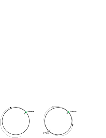
Figure 4.3: On the left side: A single D-brane (in green) transverse to a compact direction violates the p-form equation of motions since its Faraday flux lines need to close to a negative charged object of the same dimension. If an orientifold plane is also present, as shown in the right side, the configuration can respect gauge invariance by guaranteeing a total vanishing RR charge. Whenever the total charge is zero, the massless spectra of D-brane excitations coupled to closed strings is free of gravitational, gauge and mixed anomalies.

One is therefore led to consider O-8 planes, which in turn impose the involution $I\cdot\Omega$ on the spectrum of string excitations, $I$ being a reflection along the compact coordinate. To take into account of the effects of the O-8 planes, one can insert a projector in the trace that computes the one loop closed string amplitudes

$$Tr_{\mathscr{H}}\left[\left(\frac{1+I\Omega}{2}\right)q^{\frac{1}{4}L_{0}}\bar{q}^{\frac{1}{4}\bar{L}_{0}}\right]=\frac{1}{2}\mathcal{T}+\mathcal{K},$$ (4.42)

with the Klein Bottle amplitude given by

$$\mathcal{K}=\frac{1}{2}\int_{0}^{\infty}\frac{d\tau_{2}}{\tau_{2}^{11/2}\eta^{8}(q\bar{q})}(V_{8}-S_{8})(q\bar{q})W_{n}.$$ (4.43)

Now the lattice sum is restricted only to winding states

$$W_{n}=\sum_{n\in\mathbb{Z}}e^{-\pi\tau_{2}\frac{(nR)^{2}}{\alpha^{\prime}}}=\sum_{n\in\mathbb{Z}}(q\bar{q})^{\frac{1}{4\alpha^{\prime}}n^{2}R^{2}},$$ (4.44)

indeed the only states allowed to flow in $\mathcal{K}$ by the involution $I\Omega$, that selects $p_{L}=-p_{R}$.

The change of integration variable $\tau_{2}=1/2l$ gives the transverse Klein Bottle amplitude

$$\tilde{\mathcal{K}}=\frac{2^{9/2}}{2}\int\frac{dl\ l^{7/2}}{\eta(i/l)^{8}}(V_{8}-S_{8})(il)\sum_{n\in\mathbb{Z}}e^{-\pi\frac{(nR)^{2}}{2l\alpha^{\prime}}},$$ (4.45)

which after a Poisson resummation on the lattice sum

$$\sum_{n\in\mathbb{Z}}e^{-\pi\frac{(nR)^{2}}{2l\alpha^{\prime}}}=\frac{\sqrt{2\alpha^{\prime}l}}{R}\sum_{m\in\mathbb{Z}}e^{-\frac{2\pi l\alpha^{\prime}}{R^{2}}m^{2}},$$ (4.46)

and by using the modular property of the eta function $\eta(-1/\tau)=\sqrt{-i\tau_{2}}\eta(\tau)$, can be rewritten as follows

$$\tilde{\mathcal{K}}=\frac{2^{5}}{2}\int\frac{dl}{\eta(il)^{8}}(V_{8}-S_{8})(il)\sum_{m\in\mathbb{Z}}e^{-2\pi l\frac{\alpha^{\prime}}{4}\frac{(2m)^{2}}{R^{2}}}=\frac{2^{5}}{2}\int\frac{dl}{\eta(il)^{8}}(V_{8}-S_{8})(il)P_{2m}.$$ (4.47)

The open string excitations for a single stuck of D-8 branes on top of an O-8 plane gives rise to the following annulus amplitude

$$\mathcal{A}=\frac{N^{2}}{2}\int\frac{d\tau_{2}}{\tau_{2}^{11/2}\eta^{8}(i\tau_{2}/2)}(V_{8}-S_{8})(i\tau_{2}/2)\sum_{n}q^{\frac{1}{2\alpha^{\prime}}n^{2}R^{2}},$$ (4.48)

where the lattice states correspond to open strings that wind around the circle, as shown in figure 4.4.

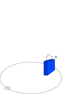
Figure 4.4: A stack of $N$ D-8 branes orthogonal to the circle. Open strings can completely wind around the circle giving rise to a tower of massive states, encoded in the lattice sum in the annulus amplitude (4.48).

The different normalisation in the lattice sum takes into account the different overall coefficient in the open string mass formula. With the change of integration variable $\tau_{2}=2/l$ we can obtain the cylinder amplitude for closed strings to propagate between two D-8 branes

$$\tilde{\mathcal{A}} = \frac{N^{2}}{2}2^{-9/2}\int\frac{dl\ l^{7/2}}{\eta(i/l)^{8}}(V_{8}-S_{8})(il)\sum_{n}e^{-\frac{2\pi}{l}\frac{n^{2}R^{2}}{\alpha^{\prime}}}$$ (4.49)

$$= 2^{-5}\frac{\sqrt{\alpha^{\prime}}}{R}\frac{N^{2}}{2}\int\frac{dl}{\eta(il)^{8}}(V_{8}-S_{8})(il)\sum_{m}e^{-2\pi l\frac{\alpha^{\prime}}{4}\frac{m^{2}}{R^{2}}}$$

$$= 2^{-5}\frac{\sqrt{\alpha^{\prime}}}{R}\frac{N^{2}}{2}\int\frac{dl}{\eta(il)^{8}}(V_{8}-S_{8})(il)\sum_{m}e^{-2\pi l\frac{\alpha^{\prime}}{4}\frac{m^{2}}{R^{2}}}$$

$$= 2^{-5}\frac{\sqrt{\alpha^{\prime}}}{R}\frac{N^{2}}{2}\int\frac{dl}{\eta(il)^{8}}(V_{8}-S_{8})(il)P_{m}.$$

The loop Möbius strip amplitude is then given by the symmetrisation under $I\Omega$ of the open string spectrum

$$\mathcal{M}=-\frac{N}{2}\int\frac{d\tau_{2}}{\tau_{2}^{11/2}\hat{\eta}^{8}(i\tau_{2}/2+1/2)}(\hat{V}_{8}-\hat{S}_{8})(i\tau_{2}/2+1/2)\sum_{n}e^{-\pi\tau_{2}\frac{1}{\alpha^{\prime}}n^{2}R^{2}},$$ (4.50)

while the transverse $\tilde{\mathcal{M}}$ corresponds to the amplitude for closed strings to propagate between a D-8 brane and a O-8 plane and is obtained from (4.49) by a change of integration variable $\tau_{2}=1/t$

$$\mathcal{M} \rightarrow -\frac{N}{2}\int\frac{dt\ t^{7/2}}{\hat{\eta}^{8}(i/2t+1/2)}(\hat{V}_{8}-\hat{S}_{8})(i/2t+1/2)\sum_{n}e^{-\frac{\pi}{t}\frac{n^{2}R^{2}}{\alpha^{\prime}}}$$ (4.51)

$$= -\frac{N}{2}\int\frac{dt\ t^{7/2}}{t^{4}\hat{\eta}^{8}(it/2+1/2)}(\hat{V}_{8}-\hat{S}_{8})(it/2+1/2)\frac{\sqrt{t}R}{\sqrt{\alpha^{\prime}}}\sum_{m}e^{-\frac{\pi t}{t}\frac{\alpha^{\prime}}{R^{2}}m^{2}}$$

$$= -\frac{R}{\sqrt{\alpha^{\prime}}}\frac{N}{2}\int\frac{dt}{\hat{\eta}^{8}(it/2+1/2)}(\hat{V}_{8}-\hat{S}_{8})(it/2+1/2)\sum_{m}e^{-\pi t\frac{\alpha^{\prime}}{R^{2}}m^{2}},$$

followed by the rescaling $t=2l$ of the horizontal proper time

$$\tilde{\mathcal{M}} = -2\frac{R}{\sqrt{\alpha^{\prime}}}\frac{N}{2}\int\frac{dl}{\hat{\eta}^{8}(il+1/2)}(\hat{V}_{8}-\hat{S}_{8})(il+1/2)\sum_{m}e^{-2\pi l\frac{\alpha^{\prime}}{4}\frac{(2m)^{2}}{R^{2}}}$$ (4.52)

$$= -2\frac{R}{\sqrt{\alpha^{\prime}}}\frac{N}{2}\int\frac{dl}{\hat{\eta}^{8}(il+1/2)}(\hat{V}_{8}-\hat{S}_{8})(il+1/2)\sum_{m}q^{\frac{\alpha^{\prime}}{4}\frac{(2m)^{2}}{R^{2}}}.$$

As usual, the factor of two in the above relation gives the correct multiplicity for the transverse diagram, while the normalisation coefficient comes out to be correctly the geometric mean between those in $\tilde{\mathcal{A}}$ and $\tilde{\mathcal{K}}$.

It is worth to notice that for consistency only those closed string states that can flow both in $\tilde{\mathcal{K}}$ and $\tilde{\mathcal{A}}$ contribute to this diagram.

Tadpole conditions can be read, as usual, by summing the coefficient in front of the massless states, flowing in the transverse diagram. Also in this case the cancellation of both RR and NSNS tadples asks for $N=32$, so that the gauge group is $SO(32)$, as for the uncompactified type I solution.

4.5 Open String Wilson Lines

Circle compactification corresponds to a non-vanishing VEV for the internal component of the metric $\langle G_{99}\rangle=R^{2}$, which is called a closed string modulus, that connects continuously a set of supersymmetric vacua preserving the original gauge group. When D-branes are present one has also the option of switching on a VEV for the internal components of the gauge boson $\langle A_{9}^{a}\rangle$ [75]. These scalars control the displacement of D-8 branes along the circle [67, 69] and, if they point into the Cartan subalgebra of the gauge group, , they do not break supersymmetry since the effective-action superpotential is proportional to the commutator of two gauge bosons.

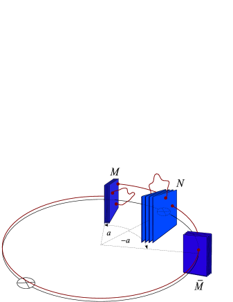
Figure 4.5:

For the configuration in fig. 4.5, the Annulus loop amplitude is

$$\mathcal{A}=(V_{8}-S_{8})\left[\left(\frac{N^{2}}{2}+M\bar{M}\right)W_{n}+NMW_{n+a}+N\bar{M}W_{n-a}+\frac{M^{2}}{2}W_{n-2a}+\frac{\bar{M}^{2}}{2}W_{n-2a}\right],$$ (4.53)

where, to lighten the notation we omit the integral over the annulus modulus $i\tau_{2}$ in the above equation.

The Möbius loop diagram is obtained by taking the unoriented open string states in the previous amplitude

$$\mathcal{M}=(\hat{V}_{8}-\hat{S}_{8})\left[\frac{N}{2}W_{n}+\left(\frac{M}{2}W_{n+2a}+\frac{\bar{M}}{2}W_{n-2a}\right)\right].$$ (4.54)

The corresponding closed string amplitudes $\tilde{\mathcal{A}}$ and $\tilde{\mathcal{M}}$ are given by a proper change of integration variables. The cylinder amplitude reads

$$\tilde{\mathcal{A}}=\frac{2^{-5}\sqrt{\alpha^{\prime}}}{2R}(V_{8}-S_{8})\left(N+Me^{2\pi iam}+\bar{M}e^{-2\pi iam}\right)^{2}P_{m},$$ (4.55)

showing clearly the displacement of the D-8 branes on the circle (see fig. 4.5).

The transverse Möbius amplitude

$$\tilde{\mathcal{M}}=\frac{\sqrt{\alpha^{\prime}}}{R}(\hat{V}_{8}-\hat{S}_{8})\left(N+Me^{4\pi iam}+\bar{M}e^{-4\pi iam}\right)P_{2m}$$ (4.56)

contains closed string states with even $m$, in agreement with $\tilde{\mathcal{K}}$ in (4.47).

In particular, massless states flowing in the open string diagrams can be read from (4.53) and (4.54) by selecting the the constant terms in the $q$ expansion of the characters

$$\mathcal{A}_{0} = (8-8)\left(\frac{N^{2}}{2}+M\bar{M}\right)$$

$$\mathcal{M}_{0} = -(8-8)\frac{N}{2}.$$ (4.57)

This shows that the original gauge group $SO(32)$ has been broken to $SO(N)\times U(M)$ with $N+2M=32$, in a way that preserves the total rank, since the total number of D-8 branes needed to cancel the total tension and charge of the O-8 planes remains the same. This phenomenon represents a nice geometrical realisation for a supersymmetry preserving Higgs mechanism: some of the originally massless gauge bosons have acquired a mass due to the minimal stretching induced by the brane displacement, as shown in the following figures.

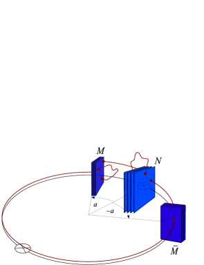
Figure 4.6: A D-brane realisation of the Higgs mechanism: brane displacement is controlled by the internal component of the gauge vector along Cartan directions (Higgs fields). If some brane is moved away from the original stuck, the open strings whose endpoints are on this brane and on a brane at the original position acquire a mass due to its minimal stretching. As a consequence the original tadpole-free gauge group is spontaneously broken $SO(32)\rightarrow SO(N)\times U(M)$, with $N+2M=32$ and $M=\bar{M}$. However, since this is a supersymmetric deformation there is not a potential for the Higgs fields, which thus represent flat directions in the moduli space.

4.6 Higher Dimensional Tori and $B_{ij}$ NSNS Discrete Moduli

We now turn to compactifications on higher dimensional tori $T^{d}$, $d>1$, corresponding to the case of non vanishing VEVs for the internal background metric components $G_{ij}$, $i,j=1,...,d$, describing the shape and the size of the target torus. Non vanishing $B_{ij}$ background values have also non-trivial effects on the zero modes of the closed string compact coordinate expansion. In the presence of orientifold planes some of the internal components of the background fields become discrete moduli giving rise to interesting effects on the open string spectra [75, 76, 77, 78, 131, 132, 130].

We choose internal coordinates along the two homology cycles of the torus $X^{i}\sim X^{i}+2\pi$, of course only in the case the cycles are mutual orthogonal, the torus metric $G_{ij}$ is diagonal in this coordinate system. With this choice of torus coordinates we know that the conjugate momenta are quantised, being integer numbers. The part of the world-sheet action that involves the compact bosonic coordinates $X^{i}$ reads

$$I=\frac{1}{2\pi\alpha^{\prime}}\int d\tau\int_{0}^{\pi}d\sigma\left(G_{ij}\partial^{\alpha}X^{i}\partial_{\alpha}X^{j}+B_{ij}\partial_{\alpha}X^{i}\partial_{\beta}X^{j}\epsilon^{\alpha\beta}\right).$$ (4.58)

One can make an ansatz for the zero mode in the internal coordinate expansion [64]

$$X^{i}_{ZM}=2n^{i}\sigma+q^{i}(\tau)$$ (4.59)

such that the same action restricted to the zero modes becomes

$$\frac{1}{2\alpha^{\prime}}\int d\tau\left(G_{ij}\dot{q}^{i}\dot{q}^{j}+2B_{ij}\dot{q}^{i}n^{j}-4G_{ij}n^{i}n^{j}\right),$$ (4.60)

with momenta given by

$$p_{i}=G_{ij}\dot{q}^{j}+2B_{ij}\dot{q}^{j}=m_{i}\in\mathbb{Z}.$$ (4.61)

Therefore

$$\dot{q}^{i}(\tau)=G^{ij}(m_{j}-2B_{ik}n^{k}),$$ (4.62)

and we obtain

$$X^{i}_{ZM}=x^{i}+\frac{1}{\alpha^{\prime}}G^{ij}(m_{j}-2B_{ik}n^{k})\tau+2n^{i}\sigma.$$ (4.63)

The left and right moving momenta are then

$$p^{i}_{L} = G^{ij}(m_{j}-B_{jk}n^{k})+n^{i}$$

$$p^{i}_{R} = G^{ij}(m_{j}+B_{jk}n^{k})-n^{i}$$ (4.64)

i.e.

$$p_{i,L} = m_{i}+(G_{ik}-B_{ik})n^{k}$$

$$p_{i,R} = m_{i}-(G_{ik}+B_{ik})n^{k}.$$ (4.65)

In this case the computation of the torus amplitude gives

$$\mathcal{T}=\int_{\mathcal{F}}\frac{d^{2}\tau}{\tau_{2}^{6}(\eta\bar{\eta})^{8}}|V_{8}-S_{8}|^{2}\ \cdot\tau_{2}^{d/2}\sum_{\vec{m},\vec{n}}\Lambda_{\vec{m},\vec{n}}^{(d)},$$ (4.66)

where the sum is now extended to a d-dimensional lattice

$$\Lambda_{\vec{m},\vec{n}}^{(d)}(\tau)=\sum_{\vec{m},\vec{n}}q^{\frac{1}{4\alpha^{\prime}}P^{2}_{R}}\bar{q}^{\frac{1}{4\alpha^{\prime}}P^{2}_{L}}.$$ (4.67)

The simplest case where we can observe the effects of a non-vanishing $B$ NSNS modulus corresponds to a compactification over a two-torus $T^{2}$ in the presence of D-7 branes transverse to the compact directions. O-7 planes, necessary to neutralise the D-7 RR charge, induce a $I_{2}\Omega(-)^{F_{L}}$ involution on the closed and open string spectra, where $I_{2}$ is a reflection along the two compact coordinates, transverse to the O-7 planes, and $F_{L}$ is the left-moving spacetime fermion numbers, which is necessary in order to have a $\mathbb{Z}_{2}$ involution [79, 80].

The closed string amplitudes are computed by

$$Tr_{\mathscr{H}}\left[\left(\frac{1+I_{2}\Omega(-)^{F_{L}}}{2}\right)q^{\frac{1}{4}L_{0}}\bar{q}^{\frac{1}{4}\bar{L}_{0}}\right]=\frac{1}{2}\mathcal{T}+\mathcal{K}.$$ (4.68)

In particular the combined effect of $\Omega$ and $I_{2}$ imposes the following condition involving the left and right momenta

$$P_{L,i}=-P_{R,i}$$ (4.69)

for the states that can flow in the Klein bottle, which via eq.(4.65) gives

$$B_{ij}n^{j}=b\epsilon_{ij}n^{j}=m_{i}.$$ (4.70)

From the above condition we see that $B$ can only be integer or half-integer, in this last case the $n^{i}$ need to be even.

We see therefore that due to the presence of the O-7 planes the $B_{ij}=b\epsilon_{ij}$ NSNS field becomes a discrete modulus [75, 76, 77, 78]. There are two possible inequivalent values for $b$, $b=0$ and $b=1/2$, since the mass formula is invariant under the transformation $b\rightarrow b+1$.

Let us consider the case of non vanishing $b=1/2$. The Klein bottle amplitude is given by

$$\mathcal{K}=\frac{1}{2}(V_{8}-S_{8})W_{2n_{1},2n_{2}},$$ (4.71)

where to lighten the notation we did not include the integral over the modulus of the double covering torus. A change in the integration variable gives $\tilde{\mathcal{K}}$, the amplitude for closed string states to propagate between two O-7 planes

$$\tilde{\mathcal{K}} = \frac{2^{5}\alpha^{\prime}}{2v_{2}}(V_{8}-S_{8})\frac{1}{4}P_{m_{1},m_{2}}$$ (4.72)

$$= \frac{2^{3}\alpha^{\prime}}{2v_{2}}(V_{8}-S_{8})\left(\frac{1+(-)^{m_{1}}+(-)^{m_{2}}-(-)^{m_{1}+m_{2}}}{2}\right)^{2}P_{m_{1},m_{2}},$$

that is obtained via a Poisson resummation on the lattice sum, after which the volume $v_{2}$ of the $T^{2}$ appears. In the second line the quantity that looks like a projector actually is a fancy way to write $1$, but it is quite instructive since it displays neatly the geometry of the O-7 planes, which in the compact space correspond to the four fixed point of the involution $I_{2}:X^{i}\rightarrow-X^{i}$
$(0,0)$, $(0,\pi)$, $(\pi,0)$ and $(\pi,\pi)$. The minus sign infront of the $(-)^{m_{1}+m_{2}}$ also indicates that the O-plane in $(\pi,\pi)$ has a reversed tension and charge with respect to the other three O-planes [78], as shown in figure (4.7).

We consider first a single stack of D-7 branes on the $(0,0)$ fixed point and lately the interesting effects arising after brane displacement on different fixed points.

In this first case, (represented in the left side of fig.4.8) , the Annulus amplitude is given by

$$\mathcal{A}=\frac{N^{2}}{2}(V_{8}-S_{8})W_{n_{1},n_{2}}$$ (4.73)

In the transverse channel the cylinder represent the amplitude for closed strings to propagate between two D-7 branes

$$\tilde{\mathcal{A}}=2^{-5}\frac{\alpha^{\prime}}{v_{2}}\frac{N^{2}}{2}(V_{8}-S_{8})P_{m_{1},m_{2}},$$ (4.74)

while the transverse Möbius $\tilde{\mathcal{M}}$ gives the amplitude for closed string states to propagate between a D-7 brane and a O-7 plane and therefore it contains only the closed string states that flow both in $\tilde{\mathcal{K}}$ and $\tilde{\mathcal{A}}$, with reflection coefficients in front of the on-shell propagators given by the geometric mean between those of the other two transverse amplitudes

$$\tilde{\mathcal{M}}=-2\frac{\alpha^{\prime}}{v_{2}}\frac{N}{4}\left(\hat{V}_{8}-\hat{S}_{8}\right)\left(\frac{1+(-)^{m_{1}}+(-)^{m_{2}}-(-)^{m_{1}+m_{2}}}{2}\right)P_{m_{1},m_{2}}.$$ (4.75)

From this last amplitude we can read a quite interesting phenomenum that is originated by the presence of a non vanishing $B$ discrete NSNS $B$ modulus. Namely the O-7 plane located at $(\pi,\pi)$ has a reversed tension and charge ( fig. 4.7) respect to the other three O-7 planes, as displayed by the negative sign in front the phase $(-)^{m_{1}+m_{2}}$. In fact $\tilde{\mathcal{M}}$ is the amplitude for propagation of closed string between a D-brane and a O-plane thus sensitive in the NSNS sector to the relative sign between the tension of these objects, while in the RR sector to the sign between their charge.

Figure 4.7: Three $O7_{+}$ planes (in green) with negative tension and charge occupy three of the four fixed point of the involution $I_{2}$, while an exotic $O7_{-}$ plane (in red) with positive tension and charge is located in the fourth fixed point.

The total tension and charge of the O-7 planes is therefore lower than for a vanishing $B=0$, a fact that can be read from the coefficient in front of the closed string states flowing in the transverse Klein bottle eq.(4.72), that in this case reads

$$\tilde{\mathcal{K}}_{0} = \frac{2^{3}\alpha^{\prime}}{2v_{2}}(V_{8}-S_{8})\left(\frac{1+(-)^{m_{1}}+(-)^{m_{2}}-(-)^{m_{1}+m_{2}}}{2}\right)^{2}P_{m_{1},m_{2}},\qquad(m_{1},m_{2})=(0,0)$$ (4.76)

$$= \left(\frac{2\sqrt{\alpha^{\prime}}}{\sqrt{v_{2}}}\right)^{2}(8-8).$$

Therefore tadpole cancellation now requires

$$\tilde{\mathcal{K}}_{0}+\tilde{\mathcal{A}}_{0}+\tilde{\mathcal{M}}_{0}=\left(2^{2}+2^{-6}N^{2}-\frac{N}{2}\right)\frac{\alpha^{\prime}}{v_{2}}(8-8)$$ (4.77)

i. e. $N=16$.

For a vanishing $B=0$ in $\tilde{\mathcal{K}}$ flow only even K.K. closed string states

$$\tilde{\mathcal{K}}_{0} = \frac{2^{3}\alpha^{\prime}}{2v_{2}}(V_{8}-S_{8})\left(\frac{1+(-)^{m_{1}}+(-)^{m_{2}}+(-)^{m_{1}+m_{2}}}{2}\right)^{2}P_{m_{1},m_{2}},\qquad(m_{1},m_{2})=(0,0)$$ (4.78)

$$= \left(\frac{2^{2}\sqrt{\alpha^{\prime}}}{\sqrt{v_{2}}}\right)^{2}(8-8),$$

so that tadpole cancellation

$$\tilde{\mathcal{K}}_{0}+\tilde{\mathcal{A}}_{0}+\tilde{\mathcal{M}}_{0}=\left(2^{4}+2^{-6}N^{2}-N\right)\frac{\alpha^{\prime}}{v_{2}}(8-8)$$ (4.79)

requires $N=32$.

Of course the reduction of the rank of the tadpole-free gauge group is the effect of a lower NSNS and RR charge due to the presence of the inverted orientifold plane.

By changing the proper time in the Möbius we recover the loop open string amplitude

$$\mathcal{M}=-\frac{N}{2}\left(\hat{V}_{8}-\hat{S}_{8}\right)\left(W_{2n_{1},2n_{2}}+W_{2n_{1}+1,2n_{2}}+W_{2n_{1},2n_{2}+1}-W_{2n_{1}+1,2n_{2}+1}\right).$$ (4.80)

From this expression and the Annuls vacuum amplitude (4.73) we can read $N^{2}/2-N/2$ states for the gauge bosons so that in this case the gauge group is $SO(16)$.

Let us now consider the case where a single stack of D-7 branes sits instead on the $(\pi,\pi)$ O-7 plane that has reversed tension and charge, as shown in the right side of figure 4.8.

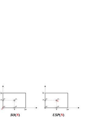
Figure 4.8: Configuration of O-planes at the fixed points of the $I_{2}$ involution. On the left side a single stuck of D-7 (red point) is on top of a O7 plane, the gauge group for the open string living on this stuck is $SO(N)$. On the right side the same stuck is on top of an exotic $O7_{-}$ plane, with postive tension and charge and thus the gauge group is $USp(N)$.

In this case the transverse Annulus reads

$$\tilde{\mathcal{A}}=2^{-5}\frac{\alpha^{\prime}}{v_{2}}\frac{(N(-)^{m_{1}+m_{2}})^{2}}{2}(V_{8}-S_{8})P_{m_{1},m_{2}},$$ (4.81)

with the factor $(-)^{m_{1}+m_{2}}$ in the square coefficient taking into account the position of the stack on the $(\pi,\pi)$ point.

In this case, there is a consequent change in the reflection coefficients of $\tilde{\mathcal{M}}$

$$\tilde{\mathcal{M}} = -2\frac{\alpha^{\prime}}{v_{2}}\frac{N}{2}\left(\hat{V}_{8}-\hat{S}_{8}\right)(-)^{m_{1}+m_{2}}\left(\frac{1+(-)^{m_{1}}+(-)^{m_{2}}-(-)^{m_{1}+m_{2}}}{2}\right)P_{m_{1},m_{2}}$$ (4.82)

$$= -2\frac{\alpha^{\prime}}{v_{2}}\frac{N}{2}\left(\hat{V}_{8}-\hat{S}_{8}\right)\left(\frac{-1+(-)^{m_{1}}+(-)^{m_{2}}+(-)^{m_{1}+m_{2}}}{2}\right)P_{m_{1},m_{2}},$$

since the coefficients in front of the propagators needs to be the geometrical means of those of the other two transverse amplitudes.

The vacuum open string amplitude $\mathcal{M}$ in this last case then reads

$$\mathcal{M}=-\frac{N}{2}\left(\hat{V}_{8}-\hat{S}_{8}\right)\left(-W_{2n_{1},2n_{2}}+W_{2n_{1}+1,2n_{2}}+W_{2n_{1},2n_{2}+1}+W_{2n_{1}+1,2n_{2}+1}\right),$$ (4.83)

From this expression and the Annuls vacuum amplitude (4.73) we can read $N^{2}/2+N/2$ states for the gauge bosons so that the gauge group is $USp(16)$. Clearly one can obtain a generic gauge group $SO(N)\times USp(2M)$ with $N+2M=16$ by displacing two stacks of branes, one on a traditional O-7 plane and the other on an inverted O-7 one. More in general, one can obtain also unitary gauge groups if some of the branes are not on top of orientifold planes, as discussed in the section dedicated to the Wilson Lines.

To summarise, the presence of a non-vanishing NSNS $B_{ij}$ has the effect of inverting tension and charge of some of the orientifold planes. On branes that are on top of reverted planes live a $USp$ gauge group, while when branes are on top of traditional O-planes, (with negative tension and charge), $SO$ gauge groups emerge [75].

All these configurations are connected continuously by varying the internal component of the vector open-string background, i.e. by moving the branes on different fixed points through continuous Wilson lines. The total tension and charge of the orientifold planes has been lowered by the $B$ background and so the total rank of the gauge group.

For a generic $T^{d}$ compactification with a non-vanishing $B_{ij}$ of rank $r$, the total rank of the gauge group is lowered to $2^{4-r/2}$. All these effects were first observed in the context of rational toroidal compactification and named originally Discrete Wilson lines [81]. We will come back on the subject in the next chapter when we will employ a similar mechanism for breaking supersymmetry without generating a vacuum energy [4].

Chapter 5 Mechanisms for Supersymmetry breaking

5.1 Brane Supersymmetry Breaking

Let us start with $D=10$ uncompactified spacetime and study the supersymmetry breaking effect induced by the presence of $\bar{D9}$ anti-branes in the background. Suppose we have $n$ $D9$ branes $(+,+)$ and $\bar{n}$ $\bar{D9}$ $(+,-)$, where the first sign denotes the tension of the object while the second its charge.

The relative signs for tensions and charges between D-branes and orientifold planes is measured by $\tilde{\mathcal{M}}$, the transverse amplitude for closed strings to propagate between a D-brane and an O-plane [84]

$$\tilde{\mathcal{M}}=\frac{2}{2}\left[(n+\bar{n})\epsilon_{NS}\hat{V}_{8}-(n-\bar{n})\epsilon_{R}\hat{S}_{8}\right].$$ (5.1)

The reversed sign in front of $\bar{n}$ in the R sector with respect to the corresponding type I amplitude, takes into account the opposite charge of the $\bar{D9}$ with respect to a $D9$.

With the different choices for the signs $\epsilon_{NS}$ and $\epsilon_{R}$ one can take into account the presence of all possible kinds of O9-planes in the background.

Type I corresponds to $\epsilon_{NS}=\epsilon_{R}=-$, with conventional $O9$ $(-,-)$ planes, while the choice $\epsilon_{NS}=\epsilon_{R}=+$ corresponds to $O9_{-}$ planes $(+,+)$, for $\epsilon_{NS}=+$ and $\epsilon_{R}=-$ we have $\bar{O9}_{-}$ $(+,-)$ and finally $\epsilon_{NS}=-$ and $\epsilon_{R}=+$ gives $\bar{O9}$ anti-orientifold planes $(-,+)$.

It is mandatory to cancel the overall RR charge in order not to violate gauge invariance, while the total tension (NSNS tadpole) of the objects in the background can be non-vanishing with the effect of breaking supersymmetry on the branes, since as previously discussed in the presence of supersymmetry all tadpoles automatically vanish [27, 28].

The transverse Klein bottle $\tilde{\mathcal{K}}$, being proportional to the square of the tension and charge of the planes, has the same expression for every kind of O-planes in the background

$$\tilde{\mathcal{K}}=\frac{2^{5}}{2}(V_{8}-S_{8}),$$ (5.2)

and therefore despite supersymmetry is broken or not on the branes by an uncancelled NSNS tadpole, it is exact in the bulk at the tree level, since the closed string amplitudes remain the same.

Due to eq. (5.1) and eq.(5.2), the transverse Annulus is

$$\tilde{\mathcal{A}} = \frac{2^{-5}}{2}\left[(n+\bar{n})^{2}V_{8}-(n-\bar{n})^{2}S_{8}\right]$$ (5.3)

$$= \frac{2^{-5}}{2}\left[(n^{2}+\bar{n}^{2})(V_{8}-S_{8})+n\bar{n}(V_{8}+S_{8})\right],$$

which displays the opposite RR charge between branes and anti-branes in the negative sign for $\bar{n}$ in the coefficient in front of $S_{8}$.

A change of the choice of proper time in the cylinder diagram gives the loop Annulus diagram, and via a modular $S$ transformation on the characters $(V_{8}+S_{8})(i/t)=(O_{8}-C_{8})(it)$, one recovers

$$\mathcal{A}=\left[\left(\frac{n^{2}}{2}+\frac{\bar{n}^{2}}{2}\right)(V_{8}-S_{8})+n\bar{n}(O_{8}-C_{8})\right],$$ (5.4)

which shows that the spectrum of open strings stretching between a D9 and anti-D9 has a reversed GSO projection [116], and therefore contains the open string tachyon. The presence of a tachyonic excitation signals the instability of the system due to the mutual attraction of the opposite charged objects.

The loop open string Möbius amplitude is as usual obtained from (5.1) form a $P$ modular tranformation and reads

$$\mathcal{M}=\frac{\epsilon_{NS}}{2}(n+\bar{n})\hat{V}_{8}-\frac{\epsilon_{R}}{2}(n-\bar{n})\hat{S}_{8}.$$ (5.5)

In the absence of anti-branes, $\bar{n}=0$, we have a tachyon free spectrum as shown by eq. (5.4). RR tadpole cancellation requires the conventional type I choice $\epsilon_{R}=-$, therefore there are two possibilities for the choice of the sign $\epsilon_{NS}$. $\epsilon_{NS}=-$ corresponds to conventional O9 planes and therefore to type I superstring. Relaxing the NSNS tadpole with the choice $\epsilon_{NS}=+$ corresponds to the presence of $\bar{O9}_{-}$ $(+,-)$ planes in the background. This configuration is not supersymmetric and the gauge boson has $N^{2}/2+N/2$ states, which corresponds to a $USp(32)$ gauge group, while the massless open string fermion remains in the anti-symmetric representation [63].

The presence of a non-vanishing total tension in the background corresponds to a non vanishing vacuum energy, which curves the spacetime. Among the solutions of the tadpole-corrected string equations of motion, there are spacetimes with an $SO(1,8)$ isometry group and a warping metric on the ninth dimension [82].

It is worth to stress again that both in the case of the presence of $\bar{D9}$ anti-branes and for the choice of reversed tension $\bar{O9}_{-}$ plane, supersymmetry is broken on the branes i.e. in the open spectrum [63, 83, 84], while the closed spectrum in the bulk remains supersymmetric at the tree level, since $\mathcal{T}$ and $\mathcal{K}$ are identical to the type I ones.

However, this is a tree level feature, since higher genus diagrams, starting from $g=3/2$, are expected to transmit the breaking of supersymmetry also to the closed string sector.

5.1.1 Breaking Supersymmetry with a Vanishing Vacuum Energy

The breaking of supersymmetry is, in one way or in another, connected to the issues of background redefinition and to the issues related to the effects of quantum string fluctuations on the background dynamics. One might avoid at least the problem of background redefinition if the mechanism that induces the breaking of supersymmetry has the virtue of not generating a vacuum energy. At the perturbative level this would imply that every single vacuum diagram, or their sum, cancels order by order [95].

Although a proper technology for computing arbitrarily high-genus diagrams is presently missing, it is at times possible to check whether this higher order corrections to the vacuum energy are vanishing or not.

In the following we will discuss a novel mechanism for supersymmetry breaking [4], that does not generate a perturbative vacuum energy. Differently to what discussed in the previous sections, in this non-supersymmetric class of backgrounds there is a cancellation of the NSNS tadpole, since an uncancelled dilaton tadpole generates a non-vanishing vacuum energy already at $g=1/2$ disk and crosscap diagrams.

The mechanism in question originates from the interactions between D-branes and both standard O-planes and exotics $O_{-}$ ones, with reversed tension and charged, whose presence is induced by a nonvanishing $B_{ij}$ NSNS discrete modulus, as discussed in the previous chapter. One of the main features of the mechanism is a deconstructions of D-branes in their NS and R elementary constituents that gives the possibility of building configurations respecting Fermi-Bose degeneracy. For a symmetric splitting of the branes we will show that the $g=1$ open string amplitudes are vanishing, and the vacuum energy does not receive one-loop contributions.

Moreover, at higher genus, although an explicit computation of the vacuum diagram is out of reach, we will show that the vacuum energy does not receive contributions as a consequence of higher genus generalisations of the well known Abstrusa Jacobi Aequatio (2.197).

Finally, we will study the stability of these configurations of D-branes and O-planes, by computing the one loop potential for open string moduli (Higgs fields), that control D-brane positions along compact directions. Unfortunately, as it is typically the case for non-supersymmetric backgrounds, there are instability directions in the potential, and the configuration with vanishing perturbative vacuum energy is not a true minimum but actually a saddle point in the moduli space.

5.2 A Prototype Six-Dimensional Example

In order to illustrate the supersymmetry breaking mechanism at work we start by considering a toroidal compactification in a rational CFT point. Let us choose a $T^{4}$ compactification of the type IIB superstring on a rigid torus at the SO(8) enhanced symmetry point. The rational point is reached by choosing for the background metric $G_{ij}$ the $SO(8)$ Cartan matrix

$$G_{ij}=\left(\begin{array}[]{cccc}2&-1&0&0\\ -1&2&-1&-1\\ 0&-1&2&0\\ 0&-1&0&2\end{array}\right),$$ (5.10)

and for the $B_{ij}$ NSNS background the adjacency matrix

$$B_{ij}=\left(\begin{array}[]{cccc}0&1&0&0\\ -1&0&1&1\\ 0&-1&0&0\\ 0&-1&0&0\end{array}\right).$$ (5.15)

The four dimensional lattice sum in the torus amplitude for the above choices reduces to the sum of characters relative to the $SO(8)$ conjugacy classes, the right factor in the following torus relation

$$\mathcal{T}=|V_{8}-S_{8}|^{2}\,\left(|O_{8}|^{2}+|V_{8}|^{2}+|S_{8}|^{2}+|C_{8}|^{2}\right)\,.$$ (5.16)

Its open string descendants were constructed long ago in [48] and exhibit all the main properties of orientifold constructions [60, 61, 62].

For rational compactifications the non trivial effects of a discrete $B_{ij}$ modulus in connection to open string Wilson lines, were first noticed in [81] and named in this context discrete Wilson lines. In this case the possibility of obtaining either orthogonal or simplectic gauge groups are related to the subtleties of the $P$ modular transformation in the Möbius amplitude, defined by eq. (3.39) and (3.40).

A world-sheet parity projection of the spectrum in (5.16) amounts to introducing the Klein-bottle amplitude

$$\mathcal{K}={\textstyle{1\over 2}}(V_{8}-S_{8})\,(O_{8}+V_{8}+S_{8}+C_{8})\,,$$ (5.17)

which describes the presence of O-9 planes in the background. The $\Omega$-invariant six-dimensional massless excitations comprise an $\mathcal{N}=(1,1)$ supergravity multiplet coupled to four vector multiplets.

In the transverse channel

$$\tilde{\mathcal{K}}={2^{4}\over 2}(V_{8}-S_{8})\,O_{8}$$ (5.18)

develops non-vanishing NSNS and RR tadpoles that require the introduction of D-branes to compensate the tension and charge of the O9-planes.

In the absence of Wilson lines, i.e. for $N$ coincident D-branes, the transverse-channel annulus amplitude is given by

$$\tilde{\mathcal{A}}={2^{-4}\over 2}\,N^{2}\,(V_{8}-S_{8})\,(O_{8}+V_{8}+S_{8}+C_{8})\,,$$ (5.19)

since the closed string states that flow in the tube are actually those in (5.16), that satisfy reflection conditions at the boundaries of the cylinder, that identify the holomorphic parts of the characters with the anti-holomorphic ones.

The above amplitude together with (5.18) implies the transverse-channel Möbius amplitude

$$\tilde{\mathcal{M}}=-N\,(\hat{V}_{8}-\hat{S}_{8})\,\hat{O}_{8}\,.$$

However, this is not the only possible choice for $\tilde{\mathcal{M}}$. The standard hatted characters for the internal lattice contribution decompose with respect to $SO(4)\times SO(4)$ according to

$$\hat{O}_{8}=\hat{O}_{4}\hat{O}_{4}-\hat{V}_{4}\hat{V}_{4}\,.$$

But following [81, 48, 48] one may introduce discrete Wilson lines to modify the $SO(4)\times SO(4)$ decomposition according to

$$\hat{O}_{8}^{\prime}=\hat{O}_{4}\hat{O}_{4}+\hat{V}_{4}\hat{V}_{4}\,,$$

and write the alternative Möbius amplitude

$$\tilde{\mathcal{M}}\,^{\prime}=-N\,(\hat{V}_{8}-\hat{S}_{8})\,\hat{O}_{8}^{\prime}\,.$$

The two different choices reflect the sign ambiguity of the reflection coefficients in the transverse Möbius amplitude and, since affect only massive modes, they lead to the same tadpole cancellation condition $N=16$ in the transverse-channel. However, a different choice for the above SO(4) decomposition does affect the open-string spectrum, since the corresponding $P$ transformation is also modified.

In fact, for the $SO(4)$ characters, $P$ interchanges $\hat{O}_{4}$ and $\hat{V}_{4}$,

$$P:\qquad\hat{O}_{8}\to-\hat{O}_{8}\,,\quad{\rm but}\quad\hat{O}_{8}^{\prime}\to+\hat{O}_{8}^{\prime}\,.$$ (5.20)

Therefore, the loop-channel annulus amplitude

$$\mathcal{A}={\textstyle{1\over 2}}\,N^{2}\,(V_{8}-S_{8})\,O_{8}$$

has two consistent (supersymmetric) projections

$$\mathcal{M}=+{\textstyle{1\over 2}}\,N\,(\hat{V}_{8}-\hat{S}_{8})\,\hat{O}_{8}\,,$$

and

$$\mathcal{M}\,^{\prime}=-{\textstyle{1\over 2}}\,N\,(\hat{V}_{8}-\hat{S}_{8})\,\hat{O}_{8}^{\prime}\,:$$

the former yields a $USp(16)$ gauge group while the latter yields an $SO(16)$ gauge group, as is clear by counting the multiplicity of states for $V_{8}$ in the two case : $(N^{2}/2+N/2)$ for $\mathcal{M}$, while $(N^{2}/2-N/2)$ choosing $\mathcal{M}^{\prime}$.

Notice, however, that one could have well decided to modify the internal lattice only in the NS or only in R sector of the D-brane [4]

$$\tilde{\mathcal{M}}\,^{\prime\prime}=-N\,\left(\hat{V}_{8}\,\hat{O}_{8}-\hat{S}_{8}\,\hat{O}_{8}^{\prime}\right)\,.$$

Tadpole conditions are again preserved, but in the direct channel

$$\mathcal{M}\,^{\prime\prime}={\textstyle{1\over 2}}\,N\,\left(\hat{V}_{8}\,\hat{O}_{8}+\hat{S}_{8}\,\hat{O}_{8}^{\prime}\right)$$

breaks supersymmetry and yields a USp(16) gauge group with fermions in the antisymmetric 120-dimensional (reducible) representation. However, a non-vanishing cosmological constant emerges at one loop, as a result of Fermi-Bose asymmetry in the open-string sector. In order to obtain a restoration of Fermi-Bose degeneracy we employ two different stacks of branes $N$ and $M$ that support different sign choices for the reflection coefficient in opposite way for the massive NS and R states

$$\tilde{\mathcal{M}} = -\left[\hat{V}_{8}\,\left(N\,\hat{O}_{8}+M\,\hat{O}_{8}^{\prime}\right)-\hat{S}_{8}\,\left(N\,\hat{O}_{8}^{\prime}+M\,\hat{O}_{8}\right)\right]\,.$$ (5.21)

$$= -\left\{(N+M)\,(\hat{V}_{8}-\hat{S}_{8})\,\hat{O}_{4}\hat{O}_{4}+\left[(N-M)\,\hat{V}_{8}-(-N+M)\,\hat{S}_{8}\right]\,\hat{V}_{4}\hat{V}_{4}\right\}.$$

As a consequence, the transverse Annulus amplitude needs to have the following form, in order for the states flowing in the transverse Möbius to have as reflection coefficients the geometrical mean between those of the Klein and the Annulus itself

$$\tilde{\mathcal{A}} = {2^{-4}\over 2}\,\left\{(N+M)^{2}\,(V_{8}-S_{8})\,\left(O_{4}O_{4}+\ldots\right)\right.$$ (5.22)

$$\left.+\left[(N-M)^{2}\,V_{8}-(-N+M)^{2}\,S_{8}\right]\left(V_{4}V_{4}+\ldots\right)\right\}\,,$$

where the dots correspond to a right combination of sums of the SO(4) decomposition of the $V_{8},S_{8},C_{8}$ internal characters allowed to flow as well in $\tilde{\mathcal{A}}$. In fact, the reflection conditions at the boundary of the cylinder identify the holomorphic and the anti-holomorphic parts of the states contained in $|O_{8}|^{2},|V_{8}|^{2},|S_{8}|^{2},|C_{8}|^{2}$ in the torus amplitude (5.16).

Through a $P$ modular transformation one recovers the loop Möbius amplitude

$$\mathcal{M}={\textstyle{1\over 2}}\,\left[\hat{V}_{8}\left(N\,\hat{O}_{8}-M\,\hat{O}_{8}^{\prime}\right)-\hat{S}_{8}\,\left(-N\,\hat{O}_{8}^{\prime}+M\,\hat{O}_{8}\right)\right]\,,$$ (5.23)

which allows to obtain the still missing combinations of characters in $\tilde{\mathcal{A}}$, via the loop channel constraint imposing for the Möbius amplitude to be the $\Omega$ projection of the annulus.

The change of proper time from the cylinder to the annulus implies the use of an S modular transformation, on the SO(4) characters $\{O_{4},V_{4},S_{4},C_{4}\}$ given by

$$S={1\over 2}\left(\matrix{+1&+1&+1&+1\cr+1&+1&-1&-1\cr+1&-1&-1&+1\cr+1&-1&+1&-1\cr}\right).$$

The complete form of the transverse Annulus that matches the loop channel constraint is

$$\tilde{\mathcal{A}} = {2^{-4}\over 2}\,\{(N+M)^{2}\,(V_{8}-S_{8})\,\left(O_{4}O_{4}+V_{4}O_{4}+S_{4}S_{4}+C_{4}S_{4}\right)$$ (5.24)

$$+ \left[(N-M)^{2}\,V_{8}-(-N+M)^{2}\,S_{8}\right]\left(V_{4}V_{4}+O_{4}V_{4}+C_{4}C_{4}+S_{4}C_{4}\right)\}$$

that indeed in the direct channel gives

$$\mathcal{A}={\textstyle{1\over 2}}\,(V_{8}-S_{8})\left[(N^{2}+M^{2})\,(O_{4}O_{4}+V_{4}V_{4})+2NM\,(O_{4}C_{4}+V_{4}S_{4})\right]\,.$$

This amplitude satisfies the request since indeed its unoriented states flow in $\mathcal{M}$.

Once again, it is worth to stress that this deformation involves only the signs for the reflection coefficients for massive states flowing in the transverse Möbius and therefore the total tadpoles, whose contributions arise only from massless closed string states flowing in the transverse diagrams, are identical to the supersymmetric case and read

$$N+M=16.$$

From the loop open string amplitudes one can read that the massless excitations on the D-branes comprise six-dimensional gauge bosons and four scalars in the adjoint of the Chan–Paton group

$$G_{CP}=USp(N)\otimes SO(M)$$

and non-chiral fermions in the anti-symmetric representation for the symplectic gauge group and in the symmetric one for the orthogonal gauge group.

For a generic choice of numbers $N$ and $M$ for the two stacks of branes, the configuration gives rise to a one loop non vanishing vacuum energy generated by the Möebius amplitude $\mathcal{M}$, since $\mathcal{A}$, $\mathcal{K}$ and $\mathcal{T}$ all vanish, being identical to the supersymmetric case.

But for a splitting of the 16 original branes in two identical sets

$$N=M=8\,,$$

also $\mathcal{M}$ vanishes being in this case proportional to $V_{8}-S_{8}$, which is zero as a consequence of the Jacobi Abstrusa identity.

In this last interesting configuration, the brane excitations give rise to the gauge group

$$G_{CP}=USp(8)\otimes SO(8)$$

with fermions in the representations $(27\oplus 1,1)\oplus(1,35\oplus 1)$.

The presence of the two singlet fermions is crucial for a consistent coupling of the non-supersymmetric matter sector to the supersymmetric bulk supergravity [87] . Although the massless D-brane excitations are as in [88] , the deformations we have employed here are different, and have the nicer feature of yielding an exact Fermi-Bose degenerate massless and massive spectrum for both the closed-string sector (that is still supersymmetric) and for the non-supersymmetric open-string sector, thus preventing any non-vanishing contribution to the one-loop vacuum energy. As we shall see, this guarantees that the contributions from genus three-half surfaces, and reasonably from generic genus-$g$ Riemann surfaces, vanish as well.

5.3 Deforming away from the rational point

We turn our attention to a generic point in the closed string moduli space, away from the rational point, and study the supersymmetry breaking mechanism for a generic $T^{2}$ compactification with a non vanishing $B_{ab}={\alpha^{\prime}\over 2}\epsilon_{ab}$ discrete background [4]. We consider the presence of D7 branes that are pointlike in the target torus and O7 planes to neutralise the overall NSNS and RR charges. The planes, pointlike in the compact space, induce the projection by $\Omega\,I_{2}\,(-1)^{F_{\rm L}}$ on both the closed and open string spectra, where $I_{2}$ denotes the inversion of the two compact coordinates and $(-1)^{F_{\rm L}}$ is the left-handed fermion index, needed in order that the projector squares to the identity [79, 80].

The torus amplitude is

$$\mathcal{T}=|V_{8}-S_{8}|^{2}\,\Lambda_{(2,2)}(B)\,,$$ (5.25)

while the Klein bottle amplitude

$$\mathcal{K}\,={\textstyle{1\over 2}}\,(V_{8}-S_{8})\,W_{2n_{1},2n_{2}}$$

involves only even windings, due to the presence of a non-vanishing (quantised) $B_{ab}$ background. In the transverse channel

$$\tilde{\mathcal{K}}\,={2^{3}\over 2}\,{\alpha^{\prime}\over R_{1}R_{2}}\,(V_{8}-S_{8})\,\left({1+(-1)^{m_{1}}+(-1)^{m_{2}}-(-1)^{m_{1}+m_{2}}\over 2}\right)^{2}\,P_{(m_{1},m_{2})}$$ (5.26)

neatly displays the geometry of the orientifold planes: three standard $O$ planes are sitting at the fixed points $(0,0)$, $(\pi R_{1},0)$ and $(0,\pi R_{2})$, while an $O^{-}$ plane with reversed tension and charge is sitting at the fourth fixed point $(\pi R_{1},\pi R_{2})$, as already discussed in sec 4.6 of the previous chapter.

On the other hand, the transverse-channel annulus amplitude

$$\tilde{\mathcal{A}}\,={2^{-5}\over 2}\,{\alpha^{\prime}\over R_{1}R_{2}}\,\left[\left(N+(-1)^{m_{1}+m_{2}}M\right)^{2}V_{8}-\left((-1)^{m_{1}+m_{2}}N+M\right)^{2}S_{8}\right]\,P_{(m_{1},m_{2})}$$ (5.27)

encodes all the relevant informations on the geometry of the D-branes. Notice that here we have decomposed the supersymmetric D-branes of the type I superstring into their elementary NS and R constituents

The corresponding transverse-channel Möbius amplitude can be unambiguously determined from (5.26) and (5.27) , and reads

$$\tilde{\mathcal{M}} = -{1\over 2}\,{\alpha^{\prime}\over R_{1}R_{2}}\,\left[\left(N+(-1)^{m_{1}+m_{2}}M\right)\hat{V}_{8}-\left((-1)^{m_{1}+m_{2}}N+M\right)\hat{S}_{8}\right]$$ (5.28)

$$\times\left({1+(-1)^{m_{1}}+(-1)^{m_{2}}-(-1)^{m_{1}+m_{2}}\over 2}\right)\,P_{(m_{1},m_{2})}\,.$$

The tadpole conditions are as in the supersymmetric case, and require

$$N+M=16\,.$$

Finally, the direct channel annulus

$$\mathcal{A}=(V_{8}-S_{8})\,\left[{\textstyle{1\over 2}}(N^{2}+M^{2})\,W_{(n_{1},n_{2})}+NM\,W_{(n_{1}+{1\over 2},n_{2}+{1\over 2})}\right]$$

and Möbius-strip

$$\tilde{\mathcal{M}} = -{\textstyle{1\over 2}}\Big{[}\left(N\,\hat{V}_{8}-M\,\hat{S}_{8}\right)\left(W_{(2n_{1},2n_{2})}+W_{(2n_{1}+1,2n_{2})}+W_{(2n_{1},2n_{2}+1)}-W_{(2n_{1}+1,2n_{2}+1)}\right)$$

$$+ \left(M\,\hat{V}_{8}-N\,\hat{S}_{8}\right)\left(-W_{(2n_{1},2n_{2})}+W_{(2n_{1}+1,2n_{2})}+W_{(2n_{1},2n_{2}+1)}+W_{(2n_{1}+1,2n_{2}+1)}\right)\Big{]}$$

amplitudes yield an eight-dimensional massless spectrum comprising gauge bosons and pairs of massless scalars in the adjoint representation of $G_{\rm CP}={\rm SO}(N)\otimes{\rm USp}(M)$, and non-chiral fermions in the (reducible) representations $({1\over 2}N(N+1),1)\oplus(1,{1\over 2}M(M-1))$.

As to the contributions of the four one-loop amplitudes to the vacuum energy, $\mathcal{T}$, $\mathcal{K}$ and $\mathcal{A}$ vanish identically as a result of Jacobi’s aequatio abstrusa. Furthermore, if the branes are split in two identical sets, i.e. if $N=M$, also $\mathcal{M}$ does not give any contribution to the cosmological constant. As we shall see in the next section, this also provides strong clues that all higher-genus vacuum amplitudes vanish.

5.4 Higher-genus amplitudes

Until now we have shown how acting with (suitable) discrete Wilson lines in the open unoriented sector and splitting the sixteen D-branes into two identical sets leads to a vanishing one-loop contribution to the vacuum energy. Of course, this is not enough, since higher-order corrections might well spoil this result. We shall now provide arguments that actually this is not the case: at any order in perturbation theory, no contributions to the vacuum energy are generated, if the branes are separated in equal sets, i.e. if $N=M$. This is obvious for closed Riemann surfaces, both oriented and unoriented, of arbitrary genus, since the closed-string sector is not affected by the deformation and therefore has the same properties as in the supersymmetric type I string case

Figure 5.1: Genus three-half Riemann surfaces with boundaries.

When boundaries are present, one has to be more careful, since the non-supersymmetric deformation might well induce non-vanishing contributions to the vacuum energy. Our claim, however, is that these are always multiplied by a numerical coefficient proportional to $(M-N)$, that vanishes for our choice of brane displacement [4]. Let us substantiate this statement with a closer look at a genus three-half amplitude. Among the surfaces with boundaries depicted in the figure let us concentrate on the one with two cross-caps and one hole. Similarly to the one-loop case, there is a particular choice for the period matrix $\Omega_{\alpha\beta}$ for which this surface describes a tree-level three-closed-string interaction diagram, weighted by the product of disc ($\mathcal{B}_{i}$) and cross-cap ($\mathcal{C}_{j}$) one-point functions of closed states, that can be read from the transverse-channel Klein-bottle, annulus and Möbius-strip amplitudes. More precisely, a formal expression for the one-disc–two-cross-caps amplitude is

$$\mathscr{R}_{[0,1,2]}=\sum_{i,j,k}\mathcal{C}_{i}\,\mathcal{C}_{j}\,\mathcal{B}_{k}\,\mathscr{N}\,{}_{ij}{}^{k}\,\mathscr{V}\,{}_{ij}{}^{k}\ \Omega_{\alpha\beta}\,,$$ (5.30)

where $[h,b,c]$ counts the number of holes $h$, boundaries $b$ and cross-caps $c$, $\mathscr{N}\,{}_{ij}{}^{k}$ are the fusion rule coefficients and $\mathscr{V}\,{}_{ij}{}^{k}(\Omega_{\alpha\beta})$ is a complicated function of the period matrix encoding the kinematics of the three-point interaction among states $i$, $j$ and $k$. This amplitude is expected to vanish in the supersymmetric (undeformed) case, and this requirement imposes some relations among the functions $\mathscr{V}\,{}_{ij}{}^{k}(\Omega_{\alpha\beta})$ that we have not defined explicitly

For instance, for the supersymmetric solution with transverse amplitudes (5.21) and (5.24)

$$\tilde{\mathcal{A}} = {2^{-4}\over 2}\,\big{[}(N+M)^{2}\,(V_{8}-S_{8})\,\left(O_{4}O_{4}+V_{4}O_{4}+S_{4}S_{4}+C_{4}S_{4}\right)$$ (5.31)

$$+ (N-M)^{2}\,(V_{8}-S_{8})\left(V_{4}V_{4}+O_{4}V_{4}+C_{4}C_{4}+S_{4}C_{4}\right)\big{]}$$

and

$$\tilde{\mathcal{M}}=-(N+M)\,(\hat{V}_{8}-\hat{S}_{8})\,\hat{O}_{4}\hat{O}_{4}-(N-M)\,(\hat{V}_{8}-\hat{S}_{8})\,\hat{V}_{4}\hat{V}_{4}\,,$$ (5.32)

the genus three-half amplitude takes the form

$$\mathscr{R}_{[0,1,2]} = {\textstyle{1\over 4}}\,(N+M)\,\left[\mathscr{V}\,{}_{111}+3\mathscr{V}\,{}_{133}+\mathscr{V}\,{}_{122}+\mathscr{V}\,{}_{144}+2\mathscr{V}\,{}_{234}\right]$$ (5.33)

$$+ {\textstyle{1\over 4}}\,(N-M)\,\left[\mathscr{V}\,{}_{122}+\mathscr{V}\,{}_{144}+2\mathscr{V}\,{}_{234}\right]\,,$$

where the relative numerical coefficients of the $\mathscr{V}$’s take into account the combinatorics of diagrams with given external states. The indices $1,2,3,4$ refer to the four characters $V_{8}\,O_{4}O_{4}$, $V_{8}\,V_{4}V_{4}$, $-S_{8}\,O_{4}O_{4}$ and $-S_{8}\,V_{4}V_{4}$, that identify the only states with a non-vanishing $\mathcal{C}_{i}$, as can be read from eq. (5.18) , and their non-vanishing fusion rule coefficients, all equal to one, are $\mathscr{N}\,{}_{111}$, $\mathscr{N}\,{}_{122}$, $\mathscr{N}\,{}_{133}$, $\mathscr{N}\,{}_{144}$ and $\mathscr{N}\,{}_{234}$, and, both in $\mathscr{V}\,$ and in $\mathscr{N}\,$, we have lowered the indices using the diagonal metric $\delta_{kl}$, since all characters in this model are self conjugate.

For a supersymmetric theory this amplitude is expected to vanish independently of brane locations, and thus the condition $\mathscr{R}_{[0,1,2]}=0$ amounts to the two constraints

$$\mathscr{V}\,{}_{111}+3\mathscr{V}\,{}_{133} = 0\,,$$

$$\mathscr{V}\,{}_{122}+\mathscr{V}\,{}_{144}+2\mathscr{V}\,{}_{234} = 0\,.$$ (5.34)

Turning to the non-supersymmetric open sector in eqs. (5.24) and (5.21) , one finds instead

$$\mathscr{R}_{[0,1,2]} = {\textstyle{1\over 4}}\,(N+M)\,\left[\mathscr{V}\,{}_{111}+3\mathscr{V}\,{}_{133}+\mathscr{V}\,{}_{122}+\mathscr{V}\,{}_{144}+2\mathscr{V}\,{}_{234}\right]$$ (5.35)

$$- {\textstyle{1\over 2}}\,(N-M)\,\left[\mathscr{V}\,{}_{122}-\mathscr{V}\,{}_{144}\right]\,,$$

since now $B_{4}=-N+M$ has a reversed sign. Using eq. (5.35) the non-vanishing contribution to the genus three-half vacuum energy would be

$$\mathscr{R}_{[0,1,2]}=-{\textstyle{1\over 2}}\,(N-M)\,\left[\mathscr{V}\,{}_{122}-\mathscr{V}\,{}_{144}\right]$$

that however vanishes if $N=M$.

Similar considerations hold for the other surfaces in figure 5.1, that are simply more involved since more $\mathscr{V}\,{}_{ij}{}^{k}$ terms contribute to them. In all cases, however, one can show that all the potential contributions are multiplied by the breaking coefficients $N-M$, that vanish for $N=M$.

It is not hard to extend these observations to the case of higher-genus amplitudes with arbitrary numbers of handles, holes and cross-caps, given a choice of period matrix that casts them in the form

$$\mathscr{R}\,_{[h,b,c]}=\sum_{\{n_{i}\},\{m_{j}\}}\,\prod_{i=1}^{c}\,\prod_{j=1}^{b}\,\mathcal{C}_{n_{i}}\,B_{m_{j}}\,\mathscr{N}\,\,{}^{[h]}{}_{n_{1}\ldots n_{c}|m_{1}\ldots m_{b}}\,\mathscr{V}\,\,{}^{[h]}_{n_{1}\ldots n_{c}|m_{1}\ldots m_{b}}(\Omega_{\alpha\beta})\,,$$ (5.36)

where $\mathscr{V}\,\,{}^{[h]}_{n_{1}\ldots n_{c}|m_{1}\ldots m_{b}}$ is a complicated expression encoding the $h$-loop interaction of $b+c$ closed strings, $\mathscr{N}\,\,{}^{[h]}{}_{n_{1}\ldots n_{c}|m_{1}\ldots m_{b}}$ are generalised Verlinde coefficients [89] , while the sum is over the closed-string states $\Phi_{\ell}$ with disc and cross-cap one-point functions $\mathcal{B}_{\ell}$ and $\mathcal{C}_{\ell}$, respectively. The expression (5.36) naturally descends from the definition of higher-genus Verlinde coefficients [89]

$$\mathscr{N}\,\,{}^{[h]}{}_{n_{1}\ldots n_{c}|m_{1}\ldots m_{b}}=\sum_{k}{S_{n_{1}k}\over S_{0k}}\ldots{S_{n_{c}k}\over S_{0k}}{S_{m_{1}k}\over S_{0k}}\ldots{S_{m_{b}k}\over S_{0k}}{1\over(S_{0k})^{2(h-1)}}\,,$$

and from the fusion algebra

$$\mathscr{N}\,\,{}_{i}\,\mathscr{N}\,\,{}_{j}=\sum_{k}\mathscr{N}\,\,{}_{ij}{}^{k}\,\mathscr{N}\,\,{}_{k}\,.$$

For instance, an amplitude $\mathscr{R}\,\,{}_{[0,4,0]}$ can be represented as a combination of two three-closed-string interaction vertices

$$\mathscr{R}\,\,_{[0,4,0]} = \sum_{i,j,k,l}\,B_{i}\,B_{j}\,B_{k}\,B_{l}\,\sum_{m}\mathscr{N}\,\,{}_{ij}{}^{m}\,\mathscr{N}\,\,{}_{mkl}\,\,\mathscr{V}\,\,^{[0]}{}_{ijkl}\,(\Omega_{\alpha\beta})$$ (5.37)

$$= \sum_{i,j,k,l}\,B_{i}\,B_{j}\,B_{k}\,B_{l}\,\sum_{n}\mathscr{N}\,\,{}_{ik}{}^{n}\,\mathscr{N}\,\,{}_{jnl}\,\,\mathscr{V}\,\,^{[0]}{}_{ijkl}\,(\Omega_{\alpha\beta})$$

$$= \sum_{i,j,k,l}\,B_{i}\,B_{j}\,B_{k}\,B_{l}\,\sum_{n}\sum_{p}\sum_{q}{S_{ip}S_{kp}S_{np}^{\dagger}\over S_{0p}}\,{S_{jq}S_{nq}S_{lq}\over S_{0q}}\,\,\mathscr{V}\,\,^{[0]}{}_{ijkl}\,(\Omega_{\alpha\beta})$$

$$= \sum_{i,j,k,l}\,B_{i}\,B_{j}\,B_{k}\,B_{l}\,\sum_{p}{S_{ip}S_{kp}S_{jp}S_{lp}\over(S_{0p})^{2}}\,\,\mathscr{V}\,\,^{[0]}{}_{ijkl}\,(\Omega_{\alpha\beta})$$

$$= \sum_{i,j,k,l}\,B_{i}\,B_{j}\,B_{k}\,B_{l}\,\mathscr{N}\,\,{}^{[0]}_{ijkl}\,\,\mathscr{V}\,\,^{[0]}{}_{ijkl}\,(\Omega_{\alpha\beta})\,,$$

and similarly for other surfaces.

Again, the only differences in the amplitudes (5.36) with respect to the supersymmetric case, where these amplitudes are supposed to vanish, are present in terms containing at least one $B_{\ell}=N-M$, and thus vanish if $N=M$.

All these considerations are not special to the rational case, and can be naturally extended to irrational models.

5.4.1 One-loop effective potential and Higgs masses

In the previous sections we have presented a new non-supersymmetric class of open-string vacua where different discrete Wilson lines are introduced in the NS and R sectors. In this class of models with vanishing NS-NS and, of course R-R tadpoles, supersymmetry is broken on the branes while it is exact at tree level in the bulk. If the branes are separated into two identical sets the closed and open-string spectra have an exact Fermi-Bose degeneracy, and thus the one-loop contribution to the cosmological constant vanishes identically. In section 5.4 we gave some qualitative arguments suggesting that higher-order perturbative contributions from surfaces with increasing numbers of holes, crosscaps and boundaries vanish as well.

Of course, String Theory calculations should be at all compatible with Field Theory results, where only massless states are taken into account. In the case at hand, it is easy to verify that the one-loop contribution to the vacuum energy vanishes identically also in Field Theory as a result of exact Fermi-Bose degeneracy of the massless degrees of freedom. However, non vanishing contributions do emerge at two loops, and possibly at higher loops.

This is not in principle inconsistent with our String Theory results. In fact, while at the one-loop level the vanishing of the Field Theory amplitudes for the massless fields is a necessary, though not sufficient, condition for the vanishing of the corresponding String Theory amplitudes, this is not the case at higher loops. In fact, one-loop amplitudes only involve a free propagation of the spectrum at each mass level and thus cancellations can only occur among states of equal mass, while at higher loops interactions must be taken into account. In Field Theory these exist only among massless fields, while in String Theory non-trivial interactions also exist among massless and massive excitations, and these do contribute to the cancellation of higher-genus amplitudes. In the Field Theory limit massless-massive interactions decouple and non-vanishing contributions to the vacuum energy may emerge. Of course, this can be checked only after complete quantitative expressions of higher-genus vacuum amplitudes in String Theory are known.

We turn now to address the problem of the stability [90] of the configuration of branes and orientifold planes. To this end we study the displacement of $N$ and $M$ branes in the eight-dimensional model of section 5.3, by studying the effect of Wilson lines, introduced in sec. 4.5 at pag. 4.5.

We consider a non vanishing background value for the internal components of the gauge vector field in the Cartan subalgebra

$$\langle A_{i}\rangle=diag\left(\frac{a_{i}}{R_{i}},...,\frac{a_{i}}{R_{i}},\frac{-a_{i}}{R_{i}},...\frac{-a_{i}}{R_{i}},\frac{b_{i}}{R_{i}},....,\frac{b_{i}}{R_{i}},\frac{-b_{i}}{R_{i}},...,\frac{b_{i}}{R_{i}}\right),$$ (5.38)

with $i=8,9$ along the $T^{2}$ directions. This $16\times 16$ matrix encodes the splitting of the two stacks $N$ and $M$, of eight branes each, into two sets $(N,\bar{N})$ and $(M,\bar{M})$, each containing four branes.

This background matrix corresponds to a pure gauge configuration for the gauge potential, obtained by a U(1) gauge transformation

$$A_{i}=-i\Lambda^{-1}\partial_{i}\Lambda,$$ (5.39)

with $\Lambda$ given by

$$\Lambda=diag\left(e^{ia_{i}y^{i}/R_{i}},...,e^{ia_{i}y^{i}/R_{i}},e^{-ia_{i}y^{i}/R_{i}},...,e^{-ia_{i}y^{i}/R_{i}},e^{ib_{i}y^{i}/R_{i}},....,e^{ib_{i}y^{i}/R_{i}},e^{-ib_{i}y^{i}/R_{i}},...,e^{-ib_{i}y^{i}/R_{i}}\right).$$ (5.40)

As shown in section 4.5, the presence of non vanishing Wilson lines manifest itself in the transverse Annulus amplitudes with the appearance of phases in the lattice sum, that neatly encode the brane displacement along the two circles on the internal $T^{2}$

$$N \rightarrow Ne^{2\pi ia_{1}m_{1}}e^{2\pi ia_{2}m_{2}}+\bar{N}e^{-2\pi ia_{1}m_{1}}e^{-2\pi ia_{2}m_{2}},$$

$$M \rightarrow Me^{2\pi ib_{1}m_{1}}e^{2\pi ib_{2}m_{2}}+\bar{M}e^{-2\pi ib_{1}m_{1}}e^{-2\pi ib_{2}m_{2}}.$$ (5.41)

These changes in the reflection coefficients in turn induce a modification in the Möbius amplitude, which, being the only amplitude responsible for the breaking of supersymmetry, generates a one-loop effective potential for the Higgs fields $a$ and $b$

$$\mathscr{V}=-\int_{0}^{\infty}\frac{dl}{\hat{\eta}^{8}(\frac{1}{2}+il)}\mathcal{V}(l,a,b).$$ (5.42)

This potential is obtained by replacing (5.41) in the Möbius amplitude (LABEL:mobiusnonsusy)

$$\mathcal{V}=-\frac{4\alpha^{\prime}}{R_{1}R_{2}}\hat{V}_{8}\cdot\{\mathscr{U}(a_{1},a_{2})-\mathscr{U}(b_{1},b_{2})\}.$$ (5.43)

The above expression takes into account the condition $N=\bar{N}=M=\bar{M}=4$ and the identity $V_{8}=S_{8}$, consequence of the Jacobi Abstrusa Aequatio (2.197) and the vanishing of $\theta_{1}(0|\tau)=0$.

The function $\mathscr{U}(a_{1},a_{2})$ is given by the following lattice sum

$$\mathscr{U}(a_{1},a_{2})=\sum_{m_{1},{m_{2}}\in\mathbb{Z}}e^{2\pi ia_{1}m_{1}}e^{2\pi ia_{2}m_{2}}(1-(-)^{m_{1}+m_{2}})e^{-2\pi l\frac{\alpha^{\prime}}{4}\frac{m_{1}^{2}}{R_{1}^{2}}}e^{-2\pi l\frac{\alpha^{\prime}}{4}\frac{m_{2}^{2}}{R_{2}^{2}}}.$$ (5.44)

In the expression (5.42) for the one-loop potential we have recollected the correct overall negative sign that we always drop for $g=1$ amplitudes in discussing supersymmetric vacua, since in this case all the amplitudes are vanishing and thus an overall sign does not matter. However, we still discard an overall normalisation coefficient in (5.43), irrelevant for the study of the behaviour of the potential.

The function $\mathscr{U}$ appearing in the integrand function (5.43), can be expressed in terms of Jacobi Theta functions

$$\theta\left[{}^{a}_{b}\right](z|\tau)=\sum_{n\in\mathbb{Z}}q^{\frac{1}{2}(n+a)^{2}}e^{2\pi i(z+b)(n+a)}\qquad q=e^{2\pi i\tau},$$ (5.45)

as follows

$$\mathscr{U}(a_{1},a_{2})=\theta\left[{}^{0}_{0}\right](a_{1}|\tilde{\tau})\theta\left[{}^{0}_{0}\right](a_{2}|\tilde{\tau})-\theta\left[{}^{0}_{\frac{1}{2}}\right](a_{1}|\tilde{\tau})\theta\left[{}^{0}_{\frac{1}{2}}\right](a_{2}|\tilde{\tau}).$$ (5.46)

Where $\tilde{\tau}=\frac{il}{2}\frac{\alpha^{\prime}}{R^{2}}$ and, for simplicity, we have chosen equal radii $R_{1}=R_{2}=R$ for the squared $T^{2}$.

We want to look for equilibrium configurations of D-branes and O-planes where the net classical forces, given by exchange of closed strings in the transverse $g=1$ diagrams, vanish. The stationary points as a function of the Higgs fields $a$ and $b$ are given by the solutions of

$$\frac{\partial}{\partial a_{1}}\mathcal{V}=\frac{\partial}{\partial a_{2}}\mathcal{V}=\frac{\partial}{\partial b_{1}}\mathcal{V}=\frac{\partial}{\partial b_{2}}\mathcal{V}=0,$$ (5.47)

that through eq. (5.43) and (5.46) translates into the following condition

$$\frac{\partial}{\partial\zeta_{i}}\mathscr{U}(\zeta_{1},\zeta_{2})=\frac{\partial}{\partial\zeta_{i}}\theta\left[{}^{0}_{0}\right](\zeta_{1}|\tilde{\tau})\theta\left[{}^{0}_{0}\right](\zeta_{2}|\tilde{\tau})-\frac{\partial}{\partial\zeta_{i}}\theta\left[{}^{0}_{\frac{1}{2}}\right](\zeta_{1}|\tilde{\tau})\theta\left[{}^{0}_{\frac{1}{2}}\right](\zeta_{2}|\tilde{\tau})=0.$$ (5.48)

From the definition (5.45) of the Jacobi functions as a power series in $q$

$$\frac{\partial}{\partial\zeta}\theta\left[{}^{0}_{0}\right](\zeta|\tilde{\tau})=\frac{\partial}{\partial\zeta}\sum_{n\in\mathbb{Z}}q^{n^{2}/2}e^{2\pi i\zeta}=2\pi i\sum_{n\in\mathbb{Z}}n\sin(2\pi\zeta n)q^{n^{2}/2}$$ (5.49)

one obtains that eq. (5.48) is satisfied for $\zeta=0,\frac{1}{2}$.

Similarly

$$\frac{\partial}{\partial\zeta}\theta\left[{}^{0}_{\frac{1}{2}}\right](\zeta|\tilde{\tau})=\frac{\partial}{\partial\zeta}\theta\left[{}^{0}_{0}\right](\zeta+1/2|\tilde{\tau})=\frac{\partial}{\partial\zeta}\sum_{n\in\mathbb{Z}}q^{n^{2}/2}e^{2\pi i(\zeta+1/2)}=2\pi i\sum_{n\in\mathbb{Z}}n\sin 2\pi(\zeta+1/2)nq^{n^{2}/2}$$ (5.50)

vanishes for $\zeta=0,\frac{1}{2}$.

We have therefore $16$ equilibrium configurations for $a_{1}$, $a_{2}$, $b_{1}$, $b_{2}$ either $0$ or $\frac{1}{2}$, corresponding to all the possible displacements of the four stacks of D-branes $N$, $\bar{N}$ ,$M$, $\bar{M}$ on the three $O$-planes located on the two circles of $T^{2}$ at $(0,0)$, $(0,\pi R)$, $(\pi R,0)$ and on the inverted plane $\bar{O}_{-}$ in $(\pi R,\pi R)$, (see figure 5.2).

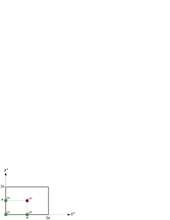
Figure 5.2: Three $O7_{+}$ planes (in green) with negative tension occupy three of the four fixed point of the involution $I_{2}$, while an exotic $O7_{-}$ plane (in red) with positive tension and charge is located in the fourth fixed point.

By writing the vanishing-argument Theta constant in the usual notation

$$\theta\left[{}^{0}_{0}\right](0|\tilde{\tau})=\theta_{3}(\tau),\qquad\theta\left[{}^{0}_{\frac{1}{2}}\right](0|\tau)=\theta_{4}(\tau),$$ (5.51)

and by using the periodicity property

$$\theta\left[{}^{0}_{\frac{1}{2}}\right]\left(\frac{1}{2}|\tau\right)=\theta\left[{}^{0}_{0}\right](0|\tau),$$ (5.52)

one can obtain the values of $\mathscr{U}(\zeta_{1},\zeta_{2})$ at the stationary points

$$\mathscr{U}(0,0) = -\ \ \mathscr{U}\left(\frac{1}{2},\frac{1}{2}\right)=\theta^{2}_{3}(\tilde{\tau})-\theta^{2}_{4}(\tilde{\tau})$$

$$\mathscr{U}\left(\frac{1}{2},0\right) = \mathscr{U}\left(0,\frac{1}{2}\right)=\theta_{3}(\tilde{\tau})\theta_{4}(\tilde{\tau})-\theta_{4}(\tilde{\tau})\theta_{3}(\tilde{\tau})=0.$$ (5.53)

Recalling from eq. (5.43) that the one loop potential is proportional to

$$\mathcal{V}\sim\mathscr{U}(a_{1},a_{2})-\mathscr{U}(b_{1},b_{2}),$$ (5.54)

it is then easy to check with the help of (5.53) that, besides the configuration of interest (0,0,0,0), the following points have a vanishing one loop energy

$$(1/2,0,1/2,0),(0,1/2,0,1/2),(1/2,0,0,1/2),(0,1/2,0,1/2),(1/2,1/2,1/2,1/2).$$ (5.55)

Whence the following configurations

$$(1/2,0,0,0),(0,1/2,0,0),(1/2,1/2,1/2,0),(1/2,1/2,0,1/2),$$ (5.56)

have a non vanishing vacuum energy, proportional to

$$\Lambda\sim-\frac{\alpha^{\prime}}{R^{2}}\int_{0}^{\infty}\frac{dl\hat{V}_{8}}{\hat{\eta}_{8}}\left(\theta^{2}_{3}(\tilde{\tau})-\theta^{2}_{4}(\tilde{\tau})\right).$$ (5.57)

In the above expression because of tadpole cancellation, the divergent contribution from the constant term in the $q=e^{-2\pi l}$ theta expansion must be discarded. This term corresponds to the tadpole contribution from the Möbius strip, responsible for the divergence in the integral in the region $l\rightarrow\infty$.

Finally, in the remaining stationary points

$$(0,0,1/2,0),(0,0,0,1/2),(1/2,0,1/2,1/2),(0,1/2,1/2,1/2),$$ (5.58)

the vacuum energy is again non vanishing and opposite in sign to (5.57)

$$\Lambda\sim+\frac{\alpha^{\prime}}{R^{2}}\int_{0}^{\infty}\frac{dl\hat{V}_{8}}{\hat{\eta}_{8}}\left(\theta^{2}_{3}(\tilde{\tau})-\theta^{2}_{4}(\tilde{\tau})\right).$$ (5.59)

In order to study the nature of the 16 equilibrium configurations one considers the Hessian matrix from the one loop potential. The off-diagonal elements of the Hessian of $\mathscr{U}(\zeta_{1},\zeta_{2})$ are given by

$$\frac{\partial^{2}}{\partial a_{1}\partial a_{2}}\mathscr{U}(a_{1},a_{2})=\frac{\partial}{\partial a_{1}}\theta\left[{}^{0}_{0}\right](a_{1}|\tilde{\tau})\frac{\partial}{\partial a_{2}}\theta\left[{}^{0}_{0}\right](a_{2}|\tilde{\tau})-\frac{\partial}{\partial a_{1}}\theta\left[{}^{0}_{\frac{1}{2}}\right](a_{1}|\tilde{\tau})\frac{\partial}{\partial a_{2}}\theta\left[{}^{0}_{\frac{1}{2}}\right](a_{2}|\tilde{\tau})$$ (5.60)

which are zero at the stationary points as a consequence of eq.(5.49) and (5.50).

Therefore in the stationary points the Hessian is already in a diagonal form.

For the non-vanishing diagonal elements we have for example

$$\frac{\partial^{2}}{\partial a_{1}^{2}}\mathscr{U}(a_{1},a_{2})=\frac{\partial^{2}}{\partial a_{1}^{2}}\theta\left[{}^{0}_{0}\right](a_{1}|\tilde{\tau})\theta\left[{}^{0}_{0}\right](a_{2}|\tilde{\tau})-\frac{\partial^{2}}{\partial a_{1}^{2}}\theta\left[{}^{0}_{\frac{1}{2}}\right](a_{1}|\tilde{\tau})\theta\left[{}^{0}_{\frac{1}{2}}\right](a_{2}|\tilde{\tau}),$$ (5.61)

which implies that

$$\frac{\partial^{2}}{\partial a_{2}^{2}}\mathscr{U}(a_{1},a_{2})=\frac{\partial^{2}}{\partial a_{1}^{2}}\mathscr{U}(a_{2},a_{1}).$$ (5.62)

With the definition $f(\zeta_{1},\zeta_{2})=\frac{\partial^{2}}{\partial\zeta_{1}^{2}}\mathscr{U}(\zeta_{1},\zeta_{2})$, one can write the Hessian matrix $\mathbb{H}$ in the simple form

$$\mathbb{H}=diag\big{(}f(a_{1},a_{2}),f(a_{2},a_{1}),-f(b_{1},b_{2}),-f(b_{2},b_{1})\big{)}.$$ (5.63)

Moreover, the periodicity property of the Jacobi Theta functions implies also that

$$f(0,0) = -f\left(\frac{1}{2},\frac{1}{2}\right)=:\lambda$$

$$f\left(\frac{1}{2},0\right) = -f\left(0,\frac{1}{2}\right)=:\mu.$$ (5.64)

Therefore we can write the $4\times 4$ $\mathbb{H}$ matrix at the 16 stationary points already in a diagonal form, in terms of the only two independent eigenvalues $\lambda$ and $\mu$

$$\lambda = \frac{\partial^{2}}{\partial a_{1}^{2}}\theta\biggl{[}{}^{0}_{0}\biggr{]}(0|\tilde{\tau})\theta\left[{}^{0}_{0}\right](0|\tilde{\tau})-\frac{\partial^{2}}{\partial a_{1}^{2}}\theta\biggl{[}{}^{0}_{\frac{1}{2}}\biggr{]}(0|\tilde{\tau})\theta\left[{}^{0}_{\frac{1}{2}}\right](0|\tilde{\tau})=2\pi\partial_{\tilde{\tau}}\left(\theta_{3}^{2}(\tilde{\tau})-\theta_{4}^{2}(\tilde{\tau})\right)$$

$$\mu = \frac{\partial^{2}}{\partial a_{1}^{2}}\theta\left[{}^{0}_{0}\right]\left(\frac{1}{2}|\tilde{\tau}\right)\theta\left[{}^{0}_{0}\right](0|\tilde{\tau})-\frac{\partial^{2}}{\partial a_{1}^{2}}\theta\left[{}^{0}_{\frac{1}{2}}\right]\left(\frac{1}{2}|\tilde{\tau}\right)\theta\left[{}^{0}_{\frac{1}{2}}\right](0|\tilde{\tau})$$ (5.65)

$$= 4\pi i\theta_{3}(\tilde{\tau})\theta_{4}(\tilde{\tau})\partial_{\tilde{\tau}}ln\left(\frac{\theta_{4}}{\theta_{3}}(\tilde{\tau})\right).$$

We are not particularly interested in the values of the two independent eigenvalues, rather in checking the sign of the eigenvalues of the Hessian matrix.

From the relations (5.63) and (5.64) it is easy to check that 14 of the 16 stationary points are saddle points. The list unfortunately includes also all the points with vanishing vacuum energy and in particular the configuration of interest, that corresponds to the point $(0,0,0,0)$, where $\mathbb{H}=diag\big{(}f(0,0),f(0,0),-f(0,0),-f(0,0)\big{)}=diag\big{(}\lambda,\lambda,-\lambda,-\lambda\big{)}$, clearly a saddle point.

The two points where the one-loop potential is extremum are $(1/2,1/2,0,0)$ and $(0,0,1/2,1/2)$ since $\mathbb{H}$ is given by $diag\big{(}\lambda,\lambda,\lambda,\lambda\big{)}$ for the first, while $diag\big{(}-\lambda,-\lambda,-\lambda,-\lambda\big{)}$ for the second. The vacuum energy is not vanishing in the true minimum for the one-loop potential, and is proportional to

$$|\Lambda|\sim\frac{\alpha^{\prime}}{R^{2}}|\int_{0}^{\infty}\frac{dl\hat{V}_{8}}{\hat{\eta}_{8}}\left(\theta^{2}_{3}(\tilde{\tau})-\theta^{2}_{4}(\tilde{\tau})\right)|.$$ (5.66)

An explicit computation of the above integral shows a runaway behaviour in the radii $R$.

Besides the instability in the radius, the above value is naturally related to the string scale $\alpha^{\prime}$ and therefore by far to high to represent the correct order of magnitude of the observed Cosmological Constant. It is also fear to remind that this is a one-loop value and, one should compute contributions from higher genus vacuum diagrams, in order to analyse in a systematic fashion the quantum effects of supersymmetry breaking and single out the true vacuum.

5.5 Breaking Supersymmetry in the Bulk: The Scherk-Schwarz Mechanism

There is a different way to break supersymmetry through compactification, the Scherk-Schwarz mechanism [91]. In field theory it corresponds to assign periodic boundary conditions to the fermionic fields along a compact cycle up to an R-symmetry of the Lagrangian. This produces a shift on the Fourier modes with respect to the bosons ones thus breaking partially or totally the supersymmetry. The easiest example corresponds to anti-periodic conditions, since the fermionic fields appear always as bilinears in every Lagrangian, and therefore this choice is compatible with the symmetries of the Action. This last case being quite similar to what we have discussed for the world-sheet spinors in the NSR superstring but this time in the target space.

A Fourier expansion for an anti-periodic field gives half integer modes, thus anti-periodic fermions on a circle have a tower of Kaluza-Klein states with masses

$$M^{2}_{m}=\frac{(m+1/2)^{2}}{R^{2}},\qquad m\in\mathbb{Z}.$$ (5.67)

This choice gives therefore a mass to all the fermions, controlled by the compactification radius $R$, with the result of breaking supersymmetry of the original uncompactified Lagrangian.

In string theory there are by far a larger spectrum of possibilities. Already at the closed string level [92] there is the possibility of mechanisms that work not only on the Kaluza-Klein momenta quantum number $m$ as in (5.67), but also on the closed string winding numbers $n$ or on both $m$ and $n$ at the same time. This latter interesting option will be described in section 5.5.4, where a computation of the one-loop potential induced by this mechanism shows interesting quantum effects of the breaking of supersymmetry on the closed string geometrical moduli.

In the presence of D-branes in the background there are even further possibilities, since depending on the geometry of the branes with respect to the SS cycle, where the twisted periodicity conditions for the fermions are imposed, it is possible either to connect a bulk gravitational non-supersymmetric sector to a gauge supersymmetric one or to break supersymmetry also on the branes [93, 94, 90].

A detailed study of the effects of the SS mechanism on general configurations of intersecting branes will be the subject of the next chapter [6], where it will be stressed how this mechanism can be used to remove undesidered non-chiral massless states in standard model-like spectra.

Here, we shall focus on the effects of the SS mechanism on the closed string spectrum, and in particular, to the study of the quantum effects induced by this breaking of supersymmetry by computing one-loop effective potentials.

5.5.1 Scherk-Schwarz on a Circle

We consider type IIB compactified on a circle $S^{1}$ of radius $R$ with anti-periodic boundary conditions for the fermions. As a consequence the fermionic modes have half-integer momentum quantum numbers, therefore naively one would expect the following Torus amplitude

$$\mathcal{T}=\int_{\mathcal{F}}\frac{d^{2}\tau}{\tau_{2}^{6}(\eta\bar{\eta})^{8}}\left(|V_{8}|^{2}+|S_{8}|^{2}\right)\sqrt{\tau_{2}}\sum_{m,n}\Lambda_{m,2n}-\int_{\mathcal{F}}\frac{d^{2}\tau}{\tau_{2}^{6}(\eta\bar{\eta})^{8}}\left(V_{8}\bar{S}_{8}+\bar{V}_{8}S_{8}\right)\sqrt{\tau_{2}}\sum_{m,n}\Lambda_{m+1/2,2n},$$ (5.68)

a modification of the circle torus amplitude (4.26), that takes into accounts for the different momenta quantum number of the bosons and the fermions. We recall the form of the lattice sum, first introduced in (4.27), that takes into account the discreetness of the left and right momenta along the circle coordinate

$$\sum_{m,n}\Lambda_{m,n}(R)=\sum_{n\in\mathbb{Z}}e^{-\pi\tau_{2}\alpha^{\prime}\left(\frac{m^{2}}{R^{2}}+\frac{(nR)^{2}}{(\alpha^{\prime})^{2}}\right)}e^{2\pi i\tau_{1}mn}.$$ (5.69)

However, (5.68) is not the complete answer for the torus amplitude, since this expression is not modular invariant. To see this one can rewrite (5.68) in the equivalent way

$$\mathcal{T} = \left(|V_{8}|^{2}+|S_{8}|^{2}\right)\Lambda_{m,2n}(R)-\left(V_{8}\bar{S}_{8}+\bar{V}_{8}S_{8}\right)\Lambda_{m+1/2,2n}(R),$$ (5.70)

$$= \frac{1}{2}|V_{8}-S_{8}|^{2}\Lambda_{m,n}(2R)+\frac{1}{2}|V_{8}+S_{8}|^{2}(-)^{m}\Lambda_{m,n}(2R),$$

where to go from the first to the second line we doubled the radius $R\rightarrow 2R$, (the meaning of this doubling will be explained in the next section), and the circle compactification lattice sum is given by

$$\sum_{m,n}(-)^{m}\Lambda_{m,n}(R)=\sum_{m,n\in\mathbb{Z}}(-)^{m}e^{-\pi\tau_{2}\alpha^{\prime}\left(\frac{m^{2}}{R^{2}}+\frac{(nR)^{2}}{(\alpha^{\prime})^{2}}\right)}e^{2\pi i\tau_{1}mn}.$$ (5.71)

While the first term in (5.68) is clearly modular invariant, being $1/2$ of the circle torus amplitude(4.26), the second terms is not invariant under a generic modular transformation. The character $V_{8}+S_{8}$ under an $S$ and $T$ transforms as

$$|V_{8}+S_{8}|\stackrel{{\scriptstyle S}}{{\leftrightarrow}}|O_{8}-C_{8}|\stackrel{{\scriptstyle T}}{{\leftrightarrow}}|O_{8}+C_{8}|.,$$ (5.72)

thus being only invariant under the subgroup of $PSL(2,\mathbb{Z})$ generated by $T$ and $ST^{2}S$.

The lattice sum (5.71) is clearly invariant under a $T:\tau_{1}\rightarrow\tau_{1}+1$, and after a Poisson resummation (4.28) over $m$, it can be rewritten as

$$\sum_{m,n}(-)^{m}\Lambda_{m,n} = \frac{R}{\sqrt{\alpha^{\prime}\tau_{2}}}\sum_{\mu,n}e^{-\frac{\pi R^{2}}{\alpha^{\prime}\tau_{2}}|n\tau+\mu+1/2|^{2}}$$ (5.73)

$$= \frac{R}{\sqrt{\alpha^{\prime}\tau_{2}}}\sum_{\mu,n}e^{-\frac{\pi R^{2}}{\alpha^{\prime}4\tau_{2}}|2n\tau+2\mu+1|^{2}}$$

$$= \frac{R}{\sqrt{\alpha^{\prime}\tau_{2}}}\sum_{p\in 2\mathbb{Z}+1}\sum_{c,d}e^{-\frac{\pi R^{2}p^{2}}{\alpha^{\prime}4\tau_{2}}|2c\tau+2d+1|^{2}}.$$

In the last line $p$ is the biggest integer contained in both the numbers $2n$ and $2\mu+1$.

Recall that a modular transformations acts on the modulus $\tau$ through $2\times 2$ $M_{cd}$ matrices

$$M_{cd}=\left(\begin{array}[]{cc}a&b\\ 2c&2d+1\end{array}\right),$$ (5.76)

in the following way

$$\tau\rightarrow\frac{a\tau+b}{2c\tau+2d+1}.$$ (5.77)

As a consequence the immaginary part $\tau_{2}$ transforms as

$$\tau_{2}\rightarrow\frac{\tau_{2}}{|2c\tau+2d+1|^{2}}=M_{cd}\tau_{2}.$$ (5.78)

Therefore in the last line of (5.73) one recognises the action of a generic matrix of this form with the last two entries, being two numbers one even and the other odd, coprime.

Clearly this constraint on the two entries of $M_{cd}$ suggests that the lattice sum (5.71)

$$\sqrt{\tau_{2}}\sum_{m,n}(-)^{m}\Lambda_{m,n}=\frac{R}{\sqrt{\alpha^{\prime}}}\sum_{p\in 2\mathbb{Z}+1}\sum_{c,d}e^{-\frac{\pi R^{2}p^{2}}{\alpha^{\prime}4M_{c,d}\tau_{2}}},$$ (5.79)

cannot be invariant under the full modular group.

Actually the set $\{M_{cd}\}$ gives a representation of a subgroup $\Gamma_{0}[2]$ of the modular group, called a congruence subgroup, since the last two entries of these matrixes are equal mod(2). The lattice sum written in the form (5.79) exhibits clearly an invariance under $\Gamma_{0}[2]$, since it contains a full orbit of the parameter $\tau$ under these class of matrixes. It turns out that $\Gamma_{0}[2]$ is generated by $T$ and $ST^{2}S$, the same two generators under which the character $V_{8}+S_{8}$ is shown by (5.72) to be invariant.

Of course this last observation also suggests that, to obtain a complete modular invariant torus amplitude, one has to include the missing orbits, namely the matrixes with the last two entries $(2c+1,2d)$ and those with $(2c+1,2d+1)$.

These matrixes are contained in two different lattice sums

$$\sum_{\mu,n}=e^{-\frac{\pi R^{2}}{\alpha^{\prime}\tau_{2}}|(n+1/2)\tau+\mu|^{2}},$$ (5.80)

and

$$\sum_{\mu,n}=e^{-\frac{\pi R^{2}}{\alpha^{\prime}\tau_{2}}|(n+1/2)\tau+(\mu+1/2)|^{2}},$$ (5.81)

The second of the previous lattice sums can be easily obtained from the first after a $T:\tau\rightarrow\tau+1$, while an $S:\tau\rightarrow-1/\tau$ transformation on the first sum gives

$$\sum_{\mu,n}e^{-\frac{\pi R^{2}|\tau|^{2}}{\alpha^{\prime}\tau_{2}}|-(n+1/2)\tau-\mu|^{2}} = \sum_{\mu,n}e^{-\frac{\pi R^{2}}{\alpha^{\prime}\tau_{2}}|-(n+1/2)+\mu\tau|^{2}},$$ (5.82)

$$= \sqrt{\tau_{2}}\frac{\sqrt{\alpha^{\prime}}}{R}\sum_{m,n}(-)^{m}\Lambda_{m,n}.$$

The last line of the previous equation can be obtained by comparing (5.71) with the second line, after the change of names $n\leftrightarrow-\mu$.

Moreover, the lattice sum in (5.80) corresponds to

$$\sum_{\mu,n}e^{-\frac{\pi R^{2}}{\alpha^{\prime}\tau_{2}}|(n+1/2)\tau+\mu|^{2}}=\sqrt{\tau_{2}}\frac{\sqrt{\alpha^{\prime}}}{R}\sum_{m,n}\Lambda_{m,n+1/2}$$ (5.83)

as it is clear again by the first line of (5.71).

While for the (5.81) we have

$$\sum_{\mu,n}e^{-\frac{\pi R^{2}}{\alpha^{\prime}\tau_{2}}|(n+1/2)\tau+\mu+1/2|^{2}}=\sqrt{\tau_{2}}\frac{\sqrt{\alpha^{\prime}}}{R}\sum_{m,n}(-)^{m}\Lambda_{m,n+1/2}.$$ (5.84)

To summarise we have shown that one needs three lattice sums in order to obtain a complete set of orbits of the full modular group, which are related as follows

$$\sqrt{\tau_{2}}\sum_{m,n}(-)^{m}\Lambda_{m,n}\stackrel{{\scriptstyle S}}{{\leftrightarrow}}\sqrt{\tau_{2}}\sum_{m,n}\Lambda_{m,n+1/2}\stackrel{{\scriptstyle T}}{{\leftrightarrow}}\sqrt{\tau_{2}}\sum_{m,n}(-)^{m}\Lambda_{m,n+1/2}$$ (5.85)

where the lattice sum on the left of the previous relation is $T$ invariant, while the one on the right is $S$ invariant.

An identical relation holds between the characters

$$|V_{8}+S_{8}|\stackrel{{\scriptstyle S}}{{\leftrightarrow}}|O_{8}-C_{8}|\stackrel{{\scriptstyle T}}{{\leftrightarrow}}|O_{8}+C_{8}|.$$ (5.86)

Altogether, the invariant modular torus amplitude is therefore

$$\mathcal{T} = \frac{1}{2}\int_{\mathcal{F}}\frac{d^{2}\tau}{\tau_{2}^{11/2}(\eta\bar{\eta})^{8}}\bigg{(}|V_{8}-S_{8}|^{2}\sum_{m,n}\Lambda_{m,n}+|V_{8}+S_{8}|^{2}\sum_{m,n}(-)^{m}\Lambda_{m,n}$$ (5.87)

$$+ |O_{8}-C_{8}|^{2}\sum_{m,n}\Lambda_{m,n+1/2}+|O_{8}+C_{8}|^{2}\sum_{m,n}(-)^{m}\Lambda_{m,n+1/2}\bigg{)}$$

After the rescaling $R\rightarrow R/2$ one can then obtain the missing part of (5.68) and write the complete modular invariant torus amplitude for type IIB compactified on a circle with anti-periodic boundary conditions for the spacetime fermions

$$\mathcal{T} = \left(|V_{8}|^{2}+|S_{8}|^{2}\right)\Lambda_{m,2n}-\left(V_{8}\bar{S}_{8}+\bar{V}_{8}S_{8}\right)\Lambda_{m+1/2,2n}$$ (5.88)

$$+ \left(|O_{8}|^{2}+|C_{8}|^{2}\right)\Lambda_{m,2n+1}-\left(O_{8}\bar{C}_{8}+\bar{O}_{8}C_{8}\right)\Lambda_{m+1/2,2n+1},$$

where to lighten the notation we have omitted the integration over the torus modulus and the contribution from the transverse bosons as well.

We see that the request of modular invariance introduces states in the spectrum with inverted GSO projection with respect to the type II ones. In particular there is an infinite tower of NSNS scalars of the form

$$e^{ip_{L}X_{L}+ip_{R}X_{R}}|0\rangle,$$ (5.89)

with quantum numbers $(0,2n+1)$. Since the conformal weights of this operator are $(\frac{\alpha^{\prime}}{2}P^{2}_{L},\frac{\alpha^{\prime}}{2}P^{2}_{R})$, for a given value of the radius $R$ this states become relevant if

$$\frac{\alpha^{\prime}}{2}(2n+1)^{2}\frac{R^{2}}{\alpha^{\prime 2}}<1$$ (5.90)

i.e. if $R<\frac{1}{2n+1}\sqrt{2\alpha^{\prime}}$. Therefore there is a critical radius $R_{c}\sim\sqrt{\alpha^{\prime}}$, below which the lowest NSNS scalar $(m=0,n=1)$ becomes tachyonic and the potential diverges.

5.5.2 Scherk-Schwarz as a freely Acting Orbifold: Momentum Shift

In the torus amplitude (5.87) we had to add the last two terms in order to achieve modular invariance. The need for introducing new states can also be understood in the general framework of orbifold constructions [37, 38]. To this aim let us first rewrite eq.(5.87),

$$\mathcal{T}=\frac{1}{2}\int_{\mathcal{F}}\frac{d^{2}\tau}{\tau_{2}^{6}(\eta\bar{\eta})^{8}}\left[|V_{8}-S_{8}|^{2}\sqrt{\tau_{2}}\sum_{m,n}\Lambda_{m,n}+\left(1+S+TS\right)\circ\left(|V_{8}+S_{8}|^{2}\sqrt{\tau_{2}}\sum_{m,n}(-)^{m}\Lambda_{m,n}\right)\right],$$ (5.91)

where we stressed the modular transformations that connect the various contributions.

Besides the last two terms that complete a closed modular orbit, the second term indeed acts as a projection on the type IIB spectrum that selects even $m$ quantum numbers for the bosons and odd ones for the fermions.

A shift operation on the circle $X\rightarrow X+\pi R$, translates on the left and right mover circle coordinates as

$$X_{R} \rightarrow X_{R}+\pi R/2,$$

$$X_{L} \rightarrow X_{L}+\pi R/2,$$ (5.92)

which is usually denoted by $A_{1}$-shift. This translation is realised on a closed string state $|m,n\rangle$ by the following operator

$$e^{ip_{R}\pi R/2+ip_{L}\pi R/2}|m,n\rangle=e^{i\left(\frac{m}{R}-\frac{nR}{\alpha^{\prime}}\right)\pi R/2+i\left(\frac{m}{R}+\frac{nR}{\alpha^{\prime}}\right)\pi R/2}|m,n\rangle=(-)^{m}|m,n\rangle.$$ (5.93)

If we denote by $\delta_{m}$ the above operation on the states, we see that the second term in (5.91) is obtained from the first by the action of the operator $\delta_{m}(-)^{F}$, and $(-)^{F}=(-)^{F_{R}+F_{L}}$ gives a minus sign to the fermionic NSR characters.

Therefore by halving the circle torus amplitude and adding the second term in (5.91) one is actually inserting a projector into the trace that computes this vacuum diagram [97, 93]

$$\mathcal{T}=\int_{\mathcal{F}}\frac{d^{2}\tau}{\tau_{2}}Tr\left(\frac{1+\delta_{m}(-)^{F}}{2}\right)q^{\frac{1}{4}L_{0}}\bar{q}^{\frac{1}{4}\bar{L}_{0}}.$$ (5.94)

However, this is not the end of the story since the above expression encodes only the first two terms of the complete torus amplitude (5.91). Actually by selecting invariant states under the action of $\delta_{m}(-)^{F}$ through the projector in (5.94) one is identifying points on the $S^{1}$ that have a distance of $\pi R$, therefore string satisfying the following boundary conditions

$$X(\sigma+\pi,\tau)=X(\sigma+,\tau)+\frac{n}{2}\cdot 2\pi R$$ (5.95)

are actually closed due to the $\delta$ identification. These twisted closed strings represent the missing states that complete the full torus amplitude that, as shown by eq. (5.87), have indeed half-integer winding numbers.

Finally, as we have seen at the beginning of the previous section, one actually recovers the correct Scherk-Schwarz modes that follow by imposing anti-periodicity for the fermions after halving the radius $R\rightarrow R/2$ of this orbifold description. This is simply explained by the fact that after the identification by $\delta$, the original circle is mapped in a circle with half of the original radius, that indeed corresponds to the physical compact part of the target space.

5.5.3 One-loop effective potentials from Scherk-Schwarz Breaking

In a circle compactification with the Scherk-Schwarz mechanism supersymmetry is broken by the asymmetry in the Kaluza-Klein excitations between spacetime bosons and fermions and it is formally recovered in the decompactification limit $R\rightarrow\infty$. However, from the torus amplitude and from the analysis of the dependence of the mass on the radius $R$ for the NSNS scalar contained in $|O_{8}|^{2}$, we already know (see (5.90)) the emergence of a tachyonic excitation in the region $R<\sqrt{\alpha^{\prime}}$. It is thus natural to ask about the behaviour of the one-loop potential amplitude as a function of $R$ [98, 99]

$$\mathscr{V}=-\frac{1}{2}\int_{\mathcal{F}}\frac{d^{2}\tau}{\tau_{2}^{6}(\eta\bar{\eta})^{8}}\left(1+S+TS\right)\circ\left(|V_{8}+S_{8}|^{2}\sqrt{\tau_{2}}\sum_{m,n}(-)^{m}\Lambda_{m,n}\right),$$ (5.96)

given by the last three terms of the torus amplitude (5.91) with a crucial global minus sign that we usually discard in writing the (vanishing) amplitudes for supersymmetric vacua.

The lattice sum after a Poisson resummation can be written as in (5.79),

$$\mathscr{V} = -\frac{R}{2\sqrt{\alpha^{\prime}}}\sum_{p\in 2\mathbb{Z}+1}\sum_{c,d}\int_{\mathcal{F}}\frac{d^{2}\tau}{\tau_{2}^{6}(\eta\bar{\eta})^{8}}\left(1+S+TS\right)\circ\left(|V_{8}+S_{8}|^{2}e^{-\frac{\pi R^{2}p^{2}}{\alpha^{\prime}4M_{c,d}\tau_{2}}}\right)$$ (5.97)

$$= -\frac{R}{2\sqrt{\alpha^{\prime}}}\sum_{p\in 2\mathbb{Z}+1}\int_{\bigcup_{c,d}M_{c,d}(\mathcal{F})}\frac{d^{2}\tau}{\tau_{2}^{6}(\eta\bar{\eta})^{8}}\left(1+S+TS\right)\circ\left(|V_{8}+S_{8}|^{2}e^{-\frac{\pi R^{2}p^{2}}{\alpha^{\prime}4\tau_{2}}}\right)$$

$$= -\frac{R}{2\sqrt{\alpha^{\prime}}}\sum_{p\in 2\mathbb{Z}+1}\int_{\Gamma_{0}[2](\mathcal{F})}\frac{d^{2}\tau}{\tau_{2}^{6}(\eta\bar{\eta})^{8}}\left(1+S+TS\right)\circ\left(|V_{8}+S_{8}|^{2}e^{-\frac{\pi R^{2}p^{2}}{\alpha^{\prime}4\tau_{2}}}\right),$$

and thus one can unfold the integration domain from the fundamental region $\mathcal{F}$ into the region $\bigcup_{c,d}M_{c,d}(\mathcal{F})$ which is the image under $\Gamma_{0}[2]/T$ of $\mathcal{F}$ shown in fig.5.3.

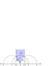
Figure 5.3: The region in light blue corresponds to the fundamental domain of $\Gamma_{0}[2]/T$: $\mathcal{F}\cup S(\mathcal{F})\cup ST(\mathcal{F})$.

Moreover by using the decomposition $\left(1+S+TS\right)\circ\Gamma_{0}[2]$ for the full modular group, one can reduce the integration domain to the half strip $\mathcal{S}=\{|\tau|>1,\ -1/2<\tau_{1}\leq 1/2,\ 0\leq\tau_{2}\}$.

$$\mathscr{V}-\frac{R}{2\sqrt{\alpha^{\prime}}}\sum_{p\in 2\mathbb{Z}+1}\int_{-1/2}^{1/2}d\tau_{1}\int_{0}^{\infty}\frac{d\tau_{2}}{\tau_{2}^{6}(\eta\bar{\eta})^{8}}\left(|V_{8}+S_{8}|^{2}e^{-\frac{\pi R^{2}p^{2}}{\alpha^{\prime}4\tau_{2}}}\right).$$ (5.98)

After this unfolding of the integration domain one then is able to perform the integral over $\tau$

$$\mathscr{V}=-\frac{R}{2\sqrt{\alpha^{\prime}}}\sum_{p\in 2\mathbb{Z}+1}\int_{0}^{\infty}\frac{d\tau_{2}}{\tau_{2}^{6}}e^{-\frac{\pi R^{2}p^{2}}{\alpha^{\prime}4\tau_{2}}}\int_{-1/2}^{1/2}d\tau_{1}\left|\frac{\theta_{2}^{2}}{\eta^{12}}\right|^{2}.$$ (5.99)

By expanding the modular functions in a $q$-power series expansion

$$\frac{\theta_{2}^{4}}{\eta^{12}}(\tau)=\sum_{N=0}^{\infty}d_{N}q^{N},$$ (5.100)

we have

$$\frac{|\theta_{2}^{4}|^{2}}{|\eta|^{24}}(\tau)=\sum_{N=0}^{\infty}\sum_{N^{\prime}=0}^{\infty}d_{N}d_{N^{\prime}}q^{N}\bar{q}^{N^{\prime}},$$ (5.101)

and therefore the $\tau_{1}$-integration gives

$$\int_{-\frac{1}{2}}^{\frac{1}{2}}d\tau_{1}\frac{|\theta_{2}^{4}|^{2}}{|\eta|^{24}}(\tau) = \sum_{N=0}^{\infty}\sum_{N^{\prime}=0}^{\infty}d_{N}d_{N^{\prime}}e^{-2\pi\tau_{2}(N+N^{\prime})}\int_{-\frac{1}{2}}^{\frac{1}{2}}d\tau_{1}e^{-2\pi i\tau_{1}(N-N^{\prime})}$$ (5.102)

$$= \sum_{N=0}^{\infty}\sum_{N^{\prime}=0}^{\infty}d_{N}d_{N^{\prime}}e^{-2\pi\tau_{2}(N+N^{\prime})}\delta_{N-N^{\prime}}=\sum_{N=0}^{\infty}d_{N}^{2}e^{-4\pi\tau_{2}N}.$$

The one-loop potential is therefore given by

$$\mathscr{V}=-\frac{R}{2\sqrt{\alpha^{\prime}}}\sum_{p\in 2\mathbb{Z}+1}\sum_{N=0}^{\infty}d_{N}^{2}\int_{0}^{\infty}\frac{d\tau_{2}}{\tau_{2}^{6}}e^{-\frac{\pi R^{2}p^{2}}{\alpha^{\prime}4\tau_{2}}-4\pi\tau_{2}N}$$ (5.103)

that can be divided into two contributions, one from the massless closed string states $N=0$ and the other from the massive states $N>0$

$$\mathscr{V}=-\frac{64R}{2\sqrt{\alpha^{\prime}}}\sum_{p\in 2\mathbb{Z}+1}\int_{0}^{\infty}\frac{d\tau_{2}}{\tau_{2}^{6}}e^{-\frac{\pi R^{2}p^{2}}{\alpha^{\prime}4\tau_{2}}}-\frac{R}{2\sqrt{\alpha^{\prime}}}\sum_{p\in 2\mathbb{Z}+1}\sum_{N=1}^{\infty}d_{N}^{2}\int_{0}^{\infty}\frac{d\tau_{2}}{\tau_{2}^{6}}e^{-\frac{\pi R^{2}p^{2}}{\alpha^{\prime}4\tau_{2}}-4\pi\tau_{2}N}.$$ (5.104)

The first integral can be calculated with the help of the formula

$$\int_{0}^{\infty}dxx^{n}e^{-\mu x}=n!/\mu^{n+1}$$ (5.105)

so that the contribution $\mathscr{V}_{0}$ from the massless states is given by [98]

$$\mathscr{V}_{0}=-\left(\frac{\sqrt{\alpha^{\prime}}}{R}\right)^{9}\frac{2^{15}\cdot 4!}{\pi^{5}}\sum_{p\in 2\mathbb{Z}+1}\frac{1}{p^{10}}=-\left(\frac{\sqrt{\alpha^{\prime}}}{R}\right)^{9}\frac{3\cdot 256\cdot 1023}{\pi^{5}}\zeta(10),$$ (5.106)

where we have computed the series in terms of the zeta-Riemann function

$$\sum_{p\in 2\mathbb{Z}+1}\frac{1}{p^{10}}=\frac{2^{10}-1}{2^{10}}\zeta(10)=\frac{1023}{1024}\zeta(10).$$ (5.107)

The contribution from the massive closed string excitations, the second integral in (5.104), is computed instead by the use of the following formula

$$\int_{0}^{\infty}dxx^{n-1}e^{-Ax-B/x}=2\left(\frac{B}{A}\right)^{n/2}K_{n}(2\sqrt{AB}),$$ (5.108)

so that

$$\mathscr{V}_{M}=-32\left(\frac{\sqrt{\alpha^{\prime}}}{R}\right)^{4}\sum_{p\in 2\mathbb{Z}+1}\sum_{N=1}^{\infty}d_{N}^{2}\frac{N^{5/2}}{p^{5}}K_{5}\left(\frac{R}{\sqrt{\alpha^{\prime}}}2\pi p\sqrt{N}\right).$$ (5.109)

For large argument the Bessel function has the following behaviour

$$K_{n}(x)\sim\frac{e^{-x}}{\sqrt{x}},$$ (5.110)

therefore for large radius $R$, the massive modes give exponentially suppressed contributions to the potential, and the leading order is given by the massless contributions, so that the potential goes to zero with a $-1/R^{9}$ behaviour, as shown in fig. 5.4

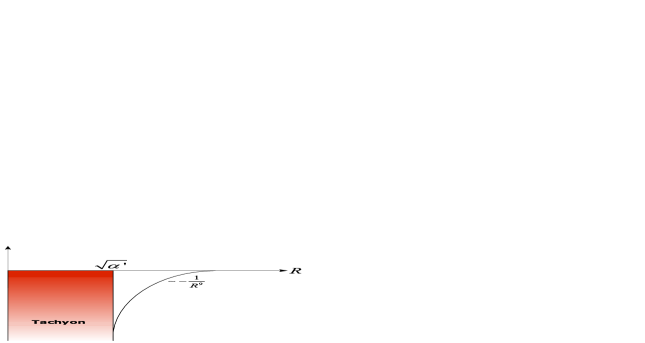
Figure 5.4: The one-loop potential in the compactification radius $R$ resulting from a momentum Scherk-Schwarz mechanism. In red the tachyonic region $R<\sqrt{\alpha^{\prime}}$ where the potential is divergent.

From the analysis of the spectrum, obtained by reading the modular invariant torus amplitude, we have seen the appearance of closed string tachyon in the region $R<\sqrt{\alpha^{\prime}}$, eq.(5.90). For these values of the radius the torus integral has an IR divergence $\tau_{2}\rightarrow\infty$, as follows from the general structure of this amplitude

$$\int_{0}^{\infty}\frac{d\tau_{2}}{\tau_{2}^{11/2}}\sum_{n}c_{N}e^{-\alpha^{\prime}M_{n}^{2}\tau_{2}},$$ (5.111)

that diverges in the presence of a tachyonic excitation.

Here we recover the same region of divergence for the potential, by considering that the number of closed string states for large $N$ grows as $d_{N}^{2}\sim\frac{e^{2\pi\sqrt{N}}}{N^{11/4}}$, while the behaviour of the Bessel functions for large $N$ is $K_{5}\sim\frac{1}{N^{1/4}}e^{-\frac{2\pi Rp}{\sqrt{\alpha^{\prime}}}\sqrt{N}}$. Therefore the sum over $N$ in the contribution (5.109) from the massive states to the potential converges only if $R/\sqrt{\alpha^{\prime}}\geq 1$.

5.5.4 Asymmetric Shifts and One-Loop potentials in various dimensions

A second possible Scherk-Schwarz mechanism consists in a breaking of the Fermi-Bose degeneracy by performing a projection on the closed string winding numbers $n$.

This second option if restricted to a pure closed string theory is connected to the mechanism on the momenta $m$, by a T-duality. Although in the presence of D-branes in the background the two options are rather distinct, giving rise to quite different and interesting effects, a subject discussed in the last chapter, here we want to focus only on the quantum effects induced by these mechanisms emerging from the computation of one-loop closed string potentials.

The winding shift mechanism can be obtained by the following asymmetric shift

$$X_{R} \rightarrow X_{R}-\pi/2R,$$

$$X_{L} \rightarrow X_{L}+\pi/2R,$$ (5.112)

usually called a $A_{3}$ shift which translates on the states

$$e^{-ip_{R}\pi R/2+ip_{L}\pi/2R}|m,n\rangle=e^{-i\left(\frac{m}{R}-\frac{nR}{\alpha^{\prime}}\right)\pi/2R+i\left(\frac{m}{R}+\frac{nR}{\alpha^{\prime}}\right)\pi/2R}|m,n\rangle=(-)^{n}|m,n\rangle.$$ (5.113)

Notice, as already anticipated, that after a T-duality along the circle coordinates

$$X_{R} \rightarrow -X_{R},$$

$$X_{L} \rightarrow X_{L},$$ (5.114)

we recover the $A_{1}$ momentum shift discussed in the previous section.

The one-loop potential for winding shift can thus be obtained from the momentum shift potential by the replacement $R\rightarrow\sqrt{\alpha^{\prime}}/R$, and its behaviour is displayed in fig. 5.5

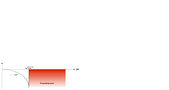
Figure 5.5: The one-loop potential in the compactification radius $R$ resulting from a winding Scherk-Schwarz mechanism. In red the tachyonic region $R>\sqrt{\alpha^{\prime}}$ where the potential is divergent.

A third interesting option is a mechanism involving momenta $m$ and winding $n$ quantum numbers at the same time, as the following selfdual asymmetric shift

$$X_{R} \rightarrow X_{R}+\pi R/2-\pi\alpha^{\prime}/2R,$$

$$X_{L} \rightarrow X_{L}+\pi R/2+\pi\alpha^{\prime}/2R.$$ (5.115)

which corresponds to $A_{1}\circ A_{3}$ and is called $A_{2}$ shift.

The level matching condition requires that one has to act simultaneously on pairs of coordinates.

5.5.5 Tachyonic regions in the moduli space for a $T^{2d}$ compactification

We want to study a general $A_{2}(-)^{F}$ asymmetric $T^{2d}$ compactification, and how the appearance of a tachyonic excitation in the spectrum depends on $d$ and the compactification moduli [5].

The modular invariant torus amplitude reads

$$\mathcal{T} = (|V_{8}|^{2}+|S_{8}|^{2})\frac{1+(-)^{(\vec{m}+\vec{n})\vec{\epsilon}}}{2}\Lambda_{\vec{m},\vec{n}}^{(2d)}+(V_{8}\bar{S}_{8}+\bar{V}_{8}S_{8})\frac{1-(-)^{(\vec{m}+\vec{n})\vec{\epsilon}}}{2}\Lambda_{\vec{m},\vec{n}}^{(2d)}$$

$$+ (|O_{8}|^{2}+|C_{8}|^{2})\frac{1+(-)^{d+(\vec{m}+\vec{n})\vec{\epsilon}}}{2}\Lambda_{\vec{m}+\vec{1}/2,\vec{n}+\vec{1}/2}^{(2d)}-(O_{8}\bar{C}_{8}+\bar{O}_{8}C_{8})\frac{1-(-)^{d+(\vec{m}+\vec{n})\vec{\epsilon}}}{2}\Lambda_{\vec{m}+\vec{1}/2,\vec{n}+\vec{1}/2}^{(2d)}.$$

The zero-mode lattice sum $\Lambda_{\vec{m},\vec{n}}^{(2d)}$, defined in (4.67), encodes the contribution to the vacuum energy from left and right moving momenta (4.65), which depend on the background moduli $G_{ij}$ and $B_{ij}$. $\vec{\epsilon}$ in eq. (LABEL:torus2d) is the $2d$ unitary vector, $\epsilon_{i}=1,\ i=1,\ldots,2d$.

Let us consider first the case of a diagonal $G_{ij}$ and vanishing $B_{ij}$, describing a torus which is the product of $2d$ circles with radii $R_{i}$, $i=1,\ldots 2d$. For this special case the generalised Scherk-Schwarz projection in (LABEL:torus2d) corresponds to the action of the asymmetric shift defined in (5.115) along the compact coordinates, since

$$e^{ip_{L,i}\left(\pi R^{i}/2+\pi\alpha^{\prime}/2R^{i}\right)+ip_{R,i}\left(\pi R^{i}/2-\pi\alpha^{\prime}/2R^{i}\right)}|\vec{m},\vec{n}\rangle=(-)^{(\vec{m}+\vec{n})\cdot\vec{\epsilon}}|\vec{m},\vec{n}\rangle.$$ (5.117)

One thus expects in this region of the moduli space the one-loop potential to enjoy the symmetry $R^{i}\rightarrow\alpha^{\prime}/R^{i}$.

Let us check whether there are relevant (tachyhonic) states in the twisted spectrum, described in the two last terms of (LABEL:torus2d). The NSNS scalars

$$e^{ip_{L,i}X^{i}_{L}+ip_{R,i}X^{i}_{R}}|0\rangle$$ (5.118)

have conformal weights $(h,h)=(\frac{\alpha^{\prime}}{2}p^{2}_{L},\frac{\alpha^{\prime}}{2}p^{2}_{R})$, with

$$p_{L,i}=\frac{m_{i}+1/2}{R^{i}}+(n_{i}+1/2)\frac{R^{i}}{\alpha^{\prime}},\qquad p_{R,i}=\frac{m_{i}+1/2}{R^{i}}-(n_{i}+1/2)\frac{R^{i}}{\alpha^{\prime}},$$ (5.119)

and $\vec{m}$ and $\vec{n}$ such that the level matching condition

$$p^{2}_{L}-p^{2}_{R}=4\left(\vec{m}+\frac{\vec{1}}{2}\right)\left(\vec{n}+\frac{\vec{1}}{2}\right)=0,$$ (5.120)

is satisfied.

The conformal weights thus satisfy the inequalty

$$h=\frac{\alpha^{\prime}}{2}p^{2}_{L}=\frac{\alpha^{\prime}}{2}p^{2}_{R}\geq d/2,$$ (5.121)

with the minimum reached for $R^{i}=\sqrt{\alpha^{\prime}}$.

It follows that the non-supersymmetric closed string spectrum obtained by the $A_{2}(-)^{F}$ mechanism for a factorizable $T^{2d}$ compactification is free of relevant modes if $2d\geq 4$, which means that the one-loop potential in this case is finite for all the values of the radii $R^{i}$. In section 5.5.7 we will consider the lowest dimensionality for the target torus where this property occurs by explicitly compute the one-loop potential and study its behaviour.

However, this appealing property of a tachyon-free spectrum for $2d\geq 4$ is restricted only for a factorisable $T^{2d}$ and disappears whenever one switches on off-diagonal metric componets and/or a $B_{ij}$ background.

In fact, to observe the presence of a tachyon region for the $T^{4}$ compactification it is enough to switch on a $B_{ij}=b\epsilon_{ij}$ along the first two directions of the torus. The zero modes in the presence of the NSNS modulus are then given by ( see eq. 4.65)

$$p_{L,i}=\frac{1}{R^{i}}(m_{i}+b\epsilon_{ij}n^{j})+n_{i}\frac{R^{i}}{\alpha^{\prime}}\qquad p_{R,i}=\frac{1}{R^{i}}(m_{i}+b\epsilon_{ij}n^{j})-n_{i}\frac{R^{i}}{\alpha^{\prime}},$$ (5.122)

for the two coordinates where the $b$ field is not zero, while

$$p_{L,i}=\frac{m_{i}}{R^{i}}+n_{i}\frac{R^{i}}{\alpha^{\prime}}\qquad p_{R,i}=\frac{m_{i}}{R^{i}}-n_{i}\frac{R^{i}}{\alpha^{\prime}},$$ (5.123)

for the other two coordinates.

The NSNS scalars (5.118) have therefore conformal weights given by

$$h = \frac{\alpha^{\prime}}{2}\bigg{[}\frac{1}{R^{2}_{1}}\left(m_{1}+\frac{1}{2}-b\left(n_{2}+\frac{1}{2}\right)\right)^{2}+\left(n_{1}+\frac{1}{2}\right)^{2}R^{2}_{1}$$ (5.124)

$$+ \frac{1}{R^{2}_{2}}\left(m_{2}+\frac{1}{2}+b\left(n_{1}+\frac{1}{2}\right)\right)^{2}+\left(n_{2}+\frac{1}{2}\right)^{2}R^{2}_{2}$$

$$+ \frac{1}{R^{2}_{3}}\left(m_{3}+\frac{1}{2}\right)^{2}+\left(n_{3}+\frac{1}{2}\right)^{2}R^{2}_{3}+\frac{1}{R^{2}_{4}}\left(m_{4}+\frac{1}{2}\right)^{2}+\left(n_{4}+\frac{1}{2}\right)^{2}R^{2}_{4}\bigg{]}.$$

For $b=1$ and $\vec{m}=\vec{n}=\vec{0}$ we have

$$h=\frac{\alpha^{\prime}}{8}\left(\frac{R^{2}_{1}+R^{2}_{2}+R^{2}_{3}+R^{2}_{4}}{(\alpha^{\prime})^{2}}+\frac{1}{R_{3}^{2}}+\frac{1}{R_{4}^{2}}\right)\geq\frac{1}{2},$$ (5.125)

thus showing the existence of the tachyonic region $1/2\leq h<1$ in the moduli space.

The reason behind the apparence of a tachyonic region for a nonvanishing $b$ is a consequence of the effect of a simultaneous shift along two or more directions on the target torus.

Recall that in the specific case of a $T^{2}$ compactification, the background data $G_{ij}$ and $B_{ij}$ can be organised to form two complex numbers encoding the shape and the volume of the $T^{2}$, the complex structure $U$ and the Kähler class $T$.

$$b=T_{1},\qquad\sqrt{detG}=T_{2},$$ (5.126)

and

$$G_{ij}=\frac{T_{2}}{U_{2}}\left(\begin{array}[]{cc}1&U_{1}\\ U_{1}&|U|^{2}\end{array}\right).$$ (5.129)

The action of a simultaneous shift on two internal coordinates changes the shape of the target $T^{2}$. In fact, it is not too difficult to show that after the identification induced by a $A_{1}$-shift a squared $T^{2}$ with modulus $U=iU_{2}=iR_{2}/R_{1}$ becomes a tilted two-torus with modulus $U^{\prime}=1/2+iR_{2}/2R_{1}$, as shown in figure 5.6.

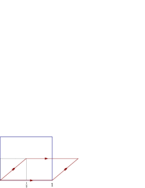
Figure 5.6: After the identification by an $A_{1}$-shift a squared $T^{2}$ with modulus $U=iU_{2}=iR_{2}/R_{1}$ becomes a tilted two-torus with modulus $U^{\prime}=1/2+iU/2$.

An $A_{3}$-shift produces an identical effect on the $T^{2}$ Kähler class, since a T-duality along one of the two coordinates interchanges $U$ with $T$, and at the same time turns an $A_{1}$-shift into an $A_{3}$-shift and vice-versa.

To summarise, if one takes a squared torus with a vanishing $b$, with Kähler class $T=iT_{2}=iR_{1}R_{2}$, and modes out by an $A_{3}$ shift, the quotient space will have a Kähler class given by $T^{\prime}=1/2+iT_{2}/2=1/2+iR_{1}R_{2}/2$. Therefore it becomes clear that by turning on a $b=1/2$ on the quotient space one is able to cancel the effect of the $A_{3}$-shift and vice-versa

Actually, in (5.125) we have observed that a $b=1$ background cancels the effects of the $A_{2}$-shift along two coordinates, thus producing a tachyonic region for small values of the corresponding radii. The fact that it occours for $b=1$ and not for $b=1/2$ is the consequence of our description of states for a tilted torus compactification in terms of (a projection of) states of a squared torus compactification. In fact, the quotient by $A_{2}=A_{1}\cdot A_{3}$ halves $T_{2}\rightarrow T_{2}/2$, the volume of the $T^{2}$. By working with the double of the $T$ modulus one expects to see the cancelation of the $A_{2}$ shift for $b=1$ and not $b=1/2$.

In order to see the same effects from a different point of view, let us recall the form of the potential For a $T^{2}$ case

$$\mathscr{V}\sim-{1\over 2}\left(1+S+TS\right)\circ\left(|V_{8}+S_{8}|^{2}\,\sum_{\vec{m},\vec{n}}(-)^{(\vec{m}+\vec{n})\cdot\vec{\epsilon}}\Lambda_{\vec{m},\vec{n}}(b,R_{1},R_{2})\right),$$ (5.130)

where in the above expression we omit the $\tau$ integration and the contributions to the potential from the transverse coordinates.

In the mass formula

$$M^{2}=\frac{(m_{1}-bn_{2})^{2}}{R_{1}^{2}}+\frac{(m_{2}+bn_{1})^{2}}{R_{2}^{2}}+n_{1}^{2}\frac{R_{1}^{2}}{(\alpha^{\prime})^{2}}+n_{1}^{2}\frac{R_{2}^{2}}{(\alpha^{\prime})^{2}},$$ (5.131)

we choose $b=1$, the potential can be rewritten as

$$\mathscr{V}=-{1\over 2}\left(1+S+TS\right)\circ\left(|V_{8}+S_{8}|^{2}\,\sum_{\vec{m}^{\prime}\vec{n}}(-)^{\vec{m}^{\prime}\cdot\vec{\epsilon}}\Lambda_{\vec{m}^{\prime},\vec{n}}(0,R_{1},R_{2})\right),$$ (5.132)

after the substitution in (5.130)

$$m_{1}-n_{2} = m_{1}^{\prime}$$

$$m_{1}+n_{2} = m_{2}^{\prime}.$$ (5.133)

Eq. (5.132) corresponds to the potential from a $A_{1}(-)^{F}$ breking mechanism, i. e. a simultaneous Scherk-Schwarz involving only Kaluza-Klein momenta. The effects of the $A_{3}$ winding shift have been cancelled by the background value $b=1$.

5.5.6 Computation of the one-loop potential from asymmetric Scherk-Schwarz $T^{2}$ compactification

We now turn to study the simplest case of a compactification on a $T^{2}$ and compute the one-loop potential generated by a $A_{2}(-)^{F}$ supersymmetry breaking mechanism [5]. In the next section we will compute the one-loop potential for a $T^{4}$ compactification, a quite interesting case, since as discussed in the previous section, for vanishing values of the compact NSNS moduli, the spectrum turns out to be tachyon-free, and the potential has a stable AdS minimum when the four $T^{4}$ radii are stabilised at the string length scale $\sqrt{\alpha^{\prime}}$.

The present $T^{2}$ case, although plagued by a tachyonic region in the compactification radii, is interesting because one is able to compute the potential in the presence of all the NSNS geometrical moduli [5].

The left and right moving momenta for a generic toroidal compactification are given by eq. (4.65), and in the $T^{2}$ case it is convenient to encode the background data $G_{ij}$ and $B_{ij}$ into two complex numbers $U$ and $T$, called the complex and Khäler structures for the two-torus, in terms of which $b=T_{1}$, $\sqrt{detG}=T_{2}$ and

$$G_{ij}=\frac{T_{2}}{U_{2}}\left(\begin{array}[]{cc}1&U_{1}\\ U_{1}&|U|^{2}\end{array}\right).$$ (5.136)

One can then check that the squares of the left and right momenta that appear in the torus amplitude can be written in terms of $U$ and $T$ as follows

$$p^{2}_{L}=p^{T}_{L}G^{-1}p_{L} = \frac{1}{T_{2}U_{2}}|Um_{1}-m_{2}-T(n_{1}+Un_{2})|^{2},$$

$$p^{2}_{R}=p^{T}_{R}G^{-1}p_{R} = \frac{1}{T_{2}U_{2}}|Um_{1}-m_{2}-\bar{T}(n_{1}+Un_{2})|^{2},$$ (5.137)

with the lattice sum given as usual by

$$\sum_{\vec{m},\vec{n}}\Lambda_{\vec{m},\vec{n}}=\sum_{\vec{m},\vec{n}}q^{\frac{\alpha^{\prime}}{4}p^{2}_{R}}\bar{q}^{\frac{\alpha^{\prime}}{4}p^{2}_{L}}.$$ (5.138)

We consider the action of the operator $V_{\vec{m},\vec{n}}$ on the two internal momenta $\vec{m}$ and winding numbers $\vec{n}$

$$V_{\vec{m},\vec{n}}|\vec{m},\vec{n}\rangle=(-)^{\vec{m}+\vec{n}}|\vec{m},\vec{n}\rangle.$$ (5.139)

The modular invariant torus amplitude therefore reads

$$\mathcal{T} = {\textstyle{1\over 2}}\sum_{\vec{m},\vec{n}}\,\Bigl{[}|V_{8}-S_{8}|^{2}\Lambda_{\vec{m},\vec{n}}+|V_{8}+S_{8}|^{2}\,(-)^{(\vec{m}+\vec{n})\cdot\vec{\epsilon}}\Lambda_{\vec{m},\vec{n}}$$

$$+ |O_{8}-C_{8}|^{2}\Lambda_{\vec{m}+{1\over 2},\vec{n}+{1\over 2}}-|O_{8}+C_{8}|^{2}\,(-)^{(\vec{m}+\vec{n})\cdot\vec{\epsilon}}\Lambda_{\vec{m}+{1\over 2},\vec{n}+{1\over 2}}\Bigr{]}$$

$$= {1\over 2}\sum_{\vec{m},\vec{n}}\,|V_{8}-S_{8}|^{2}\Lambda_{\vec{m},\vec{n}}+{1\over 2}\left(1+S+TS\right)\circ\left(|V_{8}+S_{8}|^{2}\,\sum_{\vec{m},\vec{n}}(-)^{(\vec{m}+\vec{n})\cdot\vec{\epsilon}}\Lambda_{\vec{m},\vec{n}}\right).$$

and generates the one-loop potential

$$\mathscr{V}=-\int_{\mathscr{F}}{d^{2}\tau\over\tau_{2}^{5}}{{\mathcal{T}}\over|\eta|^{16}}=-\int_{\tilde{\mathscr{F}}}{d^{2}\tau\over\tau_{2}^{5}}\left|{\theta_{2}^{4}\over\eta^{12}}\right|^{2}\sum_{\vec{m},\vec{n}}(-)^{(\vec{m}+\vec{n})\cdot\vec{\epsilon}}\Lambda_{\vec{m},\vec{n}},$$ (5.141)

where $\tilde{\mathscr{F}}=(1+S+ST)\mathscr{F}$, the region shown in figure 5.3, corresponding to a fundamental domain of $\Gamma_{0}[2]/T$. The integrand function in eq. (5.141) is invariant only under the congruence subgroup $\Gamma_{0}[2]\subset{\rm PSL}(2;\mathbb{Z})$, whose generic element has the form

$$\left(\begin{array}[]{cc}a&b\\ 2c&2d+1\end{array}\right),\qquad a(2d+1)-2cb=1.$$ (5.144)

After a Poisson resummation over the pair of Kaluza-Klein momenta $m_{1}$ and $m_{2}$ in the lattice sum, the potential can be rewritten in the following form [43]

$$\mathscr{V}=-T_{2}\int_{\tilde{\mathscr{F}}}{d^{2}\tau\over\tau_{2}^{6}}\left|{\theta_{2}^{4}\over\eta^{12}}\right|^{2}\,\sum_{\{M\}}e^{{i\pi\over 2}(1-T)\det(M)}\,\exp\left\{-{\pi T_{2}\over 4\tau_{2}U_{2}}\left|\left(\matrix{1&U\cr}\right)\,M\,\left(\matrix{\tau\cr 1\cr}\right)\right|^{2}\right\}$$ (5.145)

with $M$ an integral matrix of the form

$$M=\left(\matrix{2n_{1}&2\ell_{1}+1\cr 2n_{2}&2\ell_{2}+1\cr}\right)\,.$$

In order to unfold the integration domain from the region $\tilde{\mathscr{F}}$ into the half strip $\mathcal{S}$, where the computation of the $\tau$ integral becomes possible, one needs to decompose the space of integral matrices into orbits of the congruence subgroup $\Gamma_{0}[2]$. In this way, the sum over the set of generic matrices can be restricted to contributions from a single representative of each independent orbit and correspondingly the integration domain is enlarged from $\tilde{\mathscr{F}}$ to the image of this region under the action of $\Gamma_{0}[2]$.

In the case at hand one has to distinguish between two classes of orbits. Those generated by

$$M_{0}=\left(\matrix{0&2p+1\cr 0&2q+1\cr}\right)\,,\qquad p,q\in\mathbb{Z}$$

with vanishing determinant, and the non-degenerate orbits whose representatives can be cast into the form

$$M_{1}=\left(\matrix{2k&2p+1\cr 0&2q+1\cr}\right)\,,\qquad 2k>2p+1>0\,,\quad q\in\mathbb{Z}\,.$$

Actually, the matrices $M_{0}$ are invariant under the $T$-modular transformation, and thus generate orbits of $\Gamma_{0}[2]/T$. As a result, the integration domain unfolds in this case into the half-strip $\mathcal{S}=\Gamma_{0}[2](\tilde{\mathscr{F}})/T$, while the contribution of the non-degenerate matrices has to be integrated over two copies of the upper-half plane $\mathbb{C}_{+}=\Gamma_{0}[2](\tilde{\mathscr{F}})$.

After several pages of rather tricky computations we were able to obtain the expressions for the one-loop effective potential [5]

$$\mathscr{V}=\mathscr{V}_{0}+\mathscr{V}_{1}$$

The degenerate orbits yield

$$\mathscr{V}_{0} = -{1\over 2(4\pi^{2}\alpha^{\prime})^{4}T_{2}^{4}}\,\left[(2^{10}+1)E_{5}(U)-2^{5}E_{5}(U/2)-2^{5}E_{5}(2U)\right]$$ (5.146)

$$- {2^{8}\,T_{2}\over(2\pi)^{3}{\alpha^{\prime}}^{4}}\sum_{N=1}^{\infty}\sum_{p,q\in\mathbb{Z}}\,N^{5}\,d_{N}^{2}\,{K_{5}(y)\over y^{5}}$$

where the argument of the special Bessel function $K_{5}$ is $y=2\pi\sqrt{{NT_{2}\over U_{2}}|2p+1+U(2q+1)|^{2}}$, $d_{N}$ counts, as usual, the total degeneracy of string oscillators of mass $N$

$${V_{8}+S_{8}\over\eta^{8}}={\theta_{2}^{4}\over\eta^{12}}=\sum_{N=1}^{\infty}d_{N}\,q^{N}\,,$$

and $E_{5}(U)$ is the Eisenstein series

$$E_{2k}(U)={\Gamma(k)\over 2\pi^{k}}\,{\sum_{m,n}}^{\,\prime}{U_{2}^{k}\over|m+Un|^{2k}}\,,$$

where the primed sum does not include the point $(m,n)=(0,0)$.

Similarly the non-degenerate orbits contribute to the potential with

$$\mathscr{V}_{1}=-{(T_{2}U_{2})^{-4}\over(2\pi)^{25/2}\,{\alpha^{\prime}}^{4}}\sum_{\ell,q\in\mathbb{Z}}\sum_{N=0}^{\infty}\sum_{k=1}^{\infty}{d_{N}\,d_{|N+\ell k|}\over(2q+1)^{9}}\,e^{-i\pi(2q+1)\left[(T_{1}-1)k-(U_{1}-1)\ell\right]}\,x^{9/2}\,K_{9/2}(x)$$ (5.147)

where now the argument of the special Bessel function $K_{9/2}$ is

$$x=2\pi\sqrt{T_{2}U_{2}(2q+1)^{2}\left[N+{\textstyle{1\over 4}}\left({U_{2}\over T_{2}}\ell+{T_{2}\over U_{2}}k\right)^{2}\right]}\,.$$ (5.148)

5.5.7 Computation of the one-loop potential for asymmetric shift in a $T^{4}$ compactification

In this section we consider the computation for the one-loop potential generated by the asymmetric Scherk-Schwarz supersymmetry breaking mechanism $A_{2}(-)^{F}$ acting on a factorisable $T^{4}$. As shown in section 5.5.5, in this region of the moduli space, which corresponds to a diagonal constant metric background $G_{ij}$ and a vanishing $B_{ij}$, the closed string spectrum is free of any tachyonic excitation and, as we will show in the following, the potential has a unique negative minimum for $R^{i}=\sqrt{\alpha^{\prime}}$. This is a quite interesting result since it shows the existence of a stable AdS minimum, as the effect of moduli stabilisation induced by one-loop quantum effects. However, as already discussed in section 5.5.5, by turning on off-diagonal components of the background metric or the NSNS $B$ field one recovers tachyonic regions in the moduli space that spoil this result. A mechanism that may project out such moduli and the study of the tachyon condensation are presently under investigation.

The starting point is the expression for the quantum potential

$$\mathscr{V}=\int_{\mathscr{F}}{d^{2}\tau\over\tau_{2}^{2}}\,{1\over\tau_{2}^{4}\,|\eta|^{16}}\,\left(1+S+TS\right)\circ\left(\left|{\theta_{2}^{4}\over\eta^{4}}\right|^{2}\,\prod_{i=1}^{4}\,\tau_{2}^{2}\,\sum_{m_{i},n_{i}}\,(-)^{m_{i}}(-)^{n_{i}}\,\Lambda_{m_{i},n_{i}}\right).$$ (5.149)

In order to compute the $\tau$-integral we will follow a different path from the $T^{2}$ case, and use an ad hoc trick [107]. The reason is that in the $T^{4}$ case it is rather difficult, if not impossible, to find a decomposition of the set of matrices that one recovers after Poisson resummation of the four-dimensional lattice sum, in terms of orbits of the $\Gamma_{0}[2]$ congruence group, (see section 5.5.6 for a successful use of this technique in the computation of the potential in the $T^{2}$ case).

Therefore in the following we will describe a way-out for an apparent no-go that appears at one stage of the computation.

As usual, to evaluate $\mathscr{V}$ one needs to unfold the fundamental region

$$\mathscr{F}=\{z\in\mathbb{C}\,:\quad-{\textstyle{1\over 2}}<{\rm Re}(z)<{\textstyle{1\over 2}}\,,\quad|z|>1\},$$

into the half-strip

$$\mathscr{S}=\{z\in\mathbb{C}\,:\quad-{\textstyle{1\over 2}}<{\rm Re}(z)<{\textstyle{1\over 2}}\,,\quad 0<{\rm Im}(z)<\infty\}\,.$$ (5.150)

Although the integral on $\mathscr{S}$ extends till the dangerous region $\tau_{2}\to 0$, its convergence is ensured after a Poisson re-summation of the lattice contribution over the momenta

$$\sum_{m,n}(-)^{m}(-)^{n}\,\Lambda_{m,n}={R\over\sqrt{\tau_{2}\,\alpha^{\prime}}}\sum_{\mu,n}(-)^{n}\,e^{-{\pi R^{2}\over\alpha^{\prime}\tau_{2}}|n\tau+\mu+{1\over 2}|^{2}}\,,$$ (5.151)

or over the windings

$$\sum_{m,n}(-)^{m}(-)^{n}\,\Lambda_{m,n}=\sqrt{\alpha^{\prime}\over R^{2}\tau_{2}}\sum_{m,\nu}(-)^{m}\,e^{-{\pi\alpha^{\prime}\over R^{2}\tau_{2}}|m\tau+\nu+{1\over 2}|^{2}}\,.$$ (5.152)

These two expressions are suited to study the $R\to\infty$ and $R\to 0$ regions, respectively. Since the asymmetric shift we are using is invariant under T duality we expect identical behaviours in the two opposite regions.

Let us resum over the momenta $m$, and notice that eq. (5.151) can be conveniently rewritten (by pulling out a factor ${1\over 2}$ from the absolute value) so that only even $n$ and odd $\mu$ contribute to it. Thus, denoting by $p\in\mathbb{Z}$ the maximum integer contained in both $\mu$ and $n$, so that

$$\mu=(2d+1)\,p\,,\qquad n=2c\,p\,,\qquad{\rm with}\quad d\in\mathbb{Z},\ c\in\mathbb{N}\,,$$

one arrives at the expression

$$\sum_{m,n}(-)^{m+n}\,\Lambda_{m,n} = {R\over\sqrt{\alpha^{\prime}\tau_{2}}}\sum_{p\in 2\mathbb{Z}+1}\sum_{c\in\mathbb{N},d\in\mathbb{Z}}\,(-)^{c}\,e^{-{\pi R^{2}p^{2}\over 4\alpha^{\prime}\tau_{2}}|2c\tau+2d+1|^{2}}$$ (5.153)

$$= {R\over\sqrt{\alpha^{\prime}\tau_{2}}}\sum_{p\in 2\mathbb{Z}+1}\sum_{c\in\mathbb{N},d\in\mathbb{Z}}\,(-)^{c}\,e^{-{\pi R^{2}p^{2}\over 4\alpha^{\prime}}(M_{cd}\tau_{2})^{-1}}\,,$$

where we have introduce the matrix

$$M_{cd}=\left(\matrix{a&b\cr 2c&2d+1\cr}\right)\in{\rm PSL}(2,\mathbb{Z})\,,$$

whose projective action on the Teichmüller parameter is as usually given by

$$\tau\to M_{cd}\,\tau={a\tau+b\over 2c\tau+2d+1}\,.$$

Actually, the set of matrices $M_{cd}$ is a representation of the congruence subgroup $\Gamma_{0}[2]$ of the modular group. Recall that for a generic $n\in\mathbb{N}$, the congruence subgroup $\Gamma_{0}[n]$ is represented by matrices whose third entrance is a multiple of $n$ and the fourth one is co-prime to it.

After (5.153) is plugged into eq. (5.149), the resulting expression differs from the more conventional Scherk-Schwarz one computed in section 5.5.3 by an alternating sign $(-)^{c}$, whose origin can be traced to the stringy nature of the deformation we are now employing that simultaneously affects momenta and windings. Notice that this sign depends explicitly on $M_{cd}$, and thus its presence in the integrand could obstruct the unfolding of the fundamental domain. A careful analysis of the entire expression shows, however, that this sign disappears after the change of variable

$$\tau\to M_{cd}\,\tau$$ (5.154)

is performed. To prove this important result, we decompose $M_{cd}$ in terms of the generators $ST^{2}S$ and $T$ of $\Gamma_{0}[2]$:

$$M_{cd}=(ST^{2}S)^{k_{1}}\,T^{\ell_{1}}\,\ldots\,(ST^{2}S)^{k_{N}}\,T^{\ell_{N}}\,,$$ (5.155)

for some choice of positive or null integers $k_{i}$ and $\ell_{i}$, and with the standard representation

$$S=\left(\matrix{0&1\cr-1&0\cr}\right)\,,\qquad T=\left(\matrix{1&1\cr 0&1\cr}\right)\,,$$

for the ${\rm PSL}(2,\mathbb{Z})$ generators. A direct calculation shows that one-half of the entry $(M_{cd})_{21}$ equals the number of times the $ST^{2}S$ generator appears in the decomposition (5.155) plus an even integer number $2\mathcal{N}$

$$M_{cd}=\left(\matrix{a&b\cr 2c&2d+1\cr}\right)=(ST^{2}S)^{k_{1}}\,T^{\ell_{1}}\,\ldots\,(ST^{2}S)^{k_{N}}\,T^{\ell_{N}}=\left(\matrix{a&b\cr 2(k_{1}+\ldots+k_{N}+2\mathcal{N})&2d+1\cr}\right)\,.$$

The change of variable (5.154) then results into a series of $ST^{2}S$ and $T$ transformations on the integrand. While the latter leaves both $V_{8}+S_{8}$ and the lattice contributions invariant, the former fully compensates the alternating sign $(-)^{c}$. In fact, although under a single $ST^{2}S$ transformation $V_{8}+S_{8}$ is invariant, the three remaining lattice contributions

$$\left[\sqrt{\tau_{2}}\sum_{m,n}(-)^{m+n}\Lambda_{m,n}(\tau)\right]^{3}\stackrel{{\scriptstyle ST^{2}S}}{{\rightarrow}}-\left[\sqrt{\tau_{2}}\sum_{m,n}(-)^{m+n}\Lambda_{m,n}(\tau)\right]^{3}$$

get a minus sign, that for a generic $M_{cd}$ yields the required factor $(-)^{k_{1}+\ldots+k_{N}}=(-)^{c}$. Therefore, (5.154) maps (5.149) into

$$\mathscr{V} = {R\over\sqrt{\alpha^{\prime}}}\int_{\cup_{c,d}M_{c,d}(\mathscr{F})}\,{d^{2}\tau\over\tau_{2}^{9/2}\,|\eta|^{16}}$$ (5.156)

$$\times \left(1+S+TS\right)\circ\left[\left|{\theta_{2}^{4}\over\eta^{4}}\right|^{2}\prod_{j=2}^{4}\,\sum_{m_{j},n_{j}}(-)^{m_{j}+n_{j}}\Lambda_{m_{j},n_{j}}\sum_{p\in 2\mathbb{Z}+1}\,e^{-{\pi R^{2}p^{2}\over 2\alpha^{\prime}\tau_{2}}}\right]\,.$$

Since the integrand is invariant under $T$ modular transformations, $\tau_{2}^{\prime}=M_{cd}\,\tau_{2}$ does not depend on $a$ and $b$, and since

$$T^{m}M_{cd}=\left(\matrix{a+mc&b+md\cr 2c&2d+1\cr}\right)\,,$$

we can always shift the images $M_{cd}(\mathscr{F})$ inside the half-strip $\mathscr{S}$, so that the integration domain is now

$$\bigcup_{c,d}M_{cd}(\mathscr{F})=\Gamma_{0}[2](\mathscr{F})/T\subset\mathscr{S}\,.$$

At this point we use the residual modular transformations in (5.156) to unfold the fundamental domain into $\mathscr{S}$

$$(1+S+ST)\circ\Gamma_{0}[2](\mathscr{F})/T=\Gamma(\mathscr{F})/T=\mathscr{S}\,,$$

where we have made use of the important decomposition

$$(1+S+TS+\ldots+T^{N-1}S)\circ\Gamma_{0}[N]=\Gamma\,.$$

As a result, the potential reads

$$\mathscr{V}={2R\over\sqrt{\alpha^{\prime}}}\int_{0}^{\infty}{d\tau_{2}\over\tau_{2}^{9/2}}\int_{-1/2}^{1/2}d\tau_{1}\,\left|{\theta_{2}^{4}\over\eta^{12}}\right|^{2}\,\prod_{j=2}^{4}\,\sum_{m_{j},n_{j}}(-)^{m_{j}+n_{j}}\Lambda_{m_{j},n_{j}}\sum_{p\in 2\mathbb{N}+1}\,e^{-{\pi R^{2}p^{2}\over 2\alpha^{\prime}\tau_{2}}}\,.$$

Using the explicit expression for the lattice contributions

$$\prod_{j=2}^{4}\,\sum_{m_{j},n_{j}}(-)^{m_{j}+n_{j}}\Lambda_{m_{j},n_{j}}=\sum_{\vec{m},\vec{n}}(-)^{(\vec{m}+\vec{n})\cdot\vec{\epsilon}}\,e^{2\pi i\tau_{1}\vec{m}\cdot\vec{n}}\,e^{-\pi\alpha^{\prime}\tau_{2}\left({|\vec{m}|^{2}\over R^{2}}+|\vec{n}|^{2}{R^{2}\over\alpha^{\prime}{}^{2}}\right)}\,,$$

where now $\vec{m}$ and $\vec{n}$ are three-dimensional vectors, and the expansion

$${\vartheta_{2}^{4}\over\eta^{12}}=\sum_{N=0}^{\infty}\,d_{N}\,q^{N}\,,$$

the $\tau_{1}$ integration yields the familiar level-matching condition, so that we are left with

$$\mathscr{V}={2R\over\sqrt{\alpha^{\prime}}}\sum_{p\in 2\mathbb{N}+1}\,\sum_{\vec{m},\vec{n}}(-)^{(\vec{m}+\vec{n})\cdot\vec{\epsilon}}\,\sum_{N=0}^{\infty}\,d_{N}\,d_{N+\vec{m}\cdot\vec{n}}\,\,\Theta(N+\vec{m}\cdot\vec{n})\int_{0}^{\infty}{d\tau_{2}\over\tau_{2}^{9/2}}\,e^{-{\pi R^{2}p^{2}\over 4\alpha^{\prime}\tau_{2}}-\tau_{2}h},$$

where $\Theta(x)$ is the step function

$$\Theta(x)=\cases{1&for $x\geq 0$\cr 0&for $x<0$\cr}\,,$$

and we have defined

$$h=h(N,R,\vec{m},\vec{n})=\pi\left(4N+\alpha^{\prime}\left|{\vec{m}\over R}+{\vec{n}\,R\over\alpha^{\prime}}\right|^{2}\right)\,.$$

After the last change of variable $\tau_{2}=1/x$, the integral becomes of the form

$$\int_{0}^{\infty}dx\,x^{n-{1\over 2}}\,e^{-rx-{s\over x}}=(-)^{n}\sqrt{\pi}\,{\partial^{n}\over\partial r^{n}}\left({e^{-2\sqrt{rs}}\over\sqrt{r}}\right)\,,\qquad{\rm with}\ {\rm Re}(r),\ {\rm Re}(s)>0\,,$$

with $n=3$, $s=h$ and $r={1\over 4}\pi R^{2}p^{2}/\alpha^{\prime}$, and thus we arrive at the final expression

$$\eqalign{\mathscr{V}=&{2^{5}\,5!!\over\pi^{3}}\left({\sqrt{\alpha^{\prime}}\over R}\right)^{6}\,\sum_{\vec{m},\vec{n}}(-)^{(\vec{m}+\vec{n})\cdot\vec{\epsilon}}\,\sum_{N=0}^{\infty}\,d_{N}\,d_{N+\vec{m}\cdot\vec{n}}\,\,\Theta(N+\vec{m}\cdot\vec{n})\cr&\times\sum_{p\in 2\mathbb{N}+1}\left[{1\over p^{7}}+{f\over p^{6}}+{\textstyle{2\over 5}}{f^{2}\over p^{5}}+{\textstyle{1\over 15}}{f^{3}\over p^{4}}\right]\,e^{-pf}\cr}$$

with $f=R\sqrt{\pi h/\alpha^{\prime}}$. The contribution from the massless states, with $N=0$, $\vec{m}=\vec{n}=0$, can be exactly evaluated

$$\mathscr{V}_{0}={5!!\,2^{5}\,c_{0}^{2}\over\pi^{3}}\,\left({\sqrt{\alpha^{\prime}}\over R}\right)^{6}\sum_{p\in 2\mathbb{N}+1}{1\over p^{7}}={5!!\,2^{6}\,127\over\pi^{3}}\,\left({\sqrt{\alpha^{\prime}}\over R}\right)^{6}\,\zeta(7)\,,$$

and determines the large-radius behaviour of $\mathscr{V}$. For generic $R$, the remaining terms can be expressed in terms of poly-logarithms

$${\rm Li}_{n}(x)=\sum_{p=1}^{\infty}{x^{p}\over p^{n}}\,,$$

so that the full potential can be re-expressed as

$$\mathscr{V} = {5!!\,2^{6}\,127\over\pi^{3}}\,\left({\sqrt{\alpha^{\prime}}\over R}\right)^{6}\,\zeta(7)$$ (5.157)

$$+ {2^{4}\,5!!\over\pi^{3}}\,\left({\sqrt{\alpha^{\prime}}\over R}\right)^{6}\sum_{\{\vec{m},\vec{n}\}\not=\{0,0\}}(-)^{(\vec{m}+\vec{n})\cdot\vec{\epsilon}}\,\sum_{N}\,d_{N}\,d_{N+\vec{m}\cdot\vec{n}}\,\Theta(N+\vec{m}\cdot\vec{n})$$

$$\times \Biggl{[}{\rm Li}_{7}(e^{-f})+f\,{\rm Li}_{6}(e^{-f})+{\textstyle{2\over 5}}\,f^{2}\,{\rm Li}_{5}(e^{-f})$$

$$+ {\textstyle{1\over 15}}\,f^{3}\,{\rm Li}_{4}(e^{-f})-{\rm Li}_{7}(-e^{-\pi f})-f\,{\rm Li}_{6}(-e^{-f})$$

$$- {\textstyle{2\over 5}}\,f^{2}\,{\rm Li}_{5}(-e^{-f})-{\textstyle{1\over 15}}\,f^{3}\,{\rm Li}_{4}(-e^{-f})\Biggr{]}\,.$$

To determine the $R\to 0$ behaviour, one can notice that our starting expression is invariant under the T-duality $R\to\alpha^{\prime}/R$, and thus one would expect

$$\mathscr{V}\sim{5!!\,2^{6}\,127\over\pi^{3}}\,\left({R\over\sqrt{\alpha^{\prime}}}\right)^{6}\,\zeta(7)\,.$$

Although this result can be obtained from the final expression for the potential (5.157) after a careful summation of an infinite number of terms, it can be more easily derived if we started with a winding re-summation, as in (5.152).

Due to the absence of a tachyonic excitation in the moduli space of a factorisable $T^{4}$, the potential is a finite continuous negative function of the four radii $R^{i}/i=1,\ldots,4$.

Let us study its behaviour as a function of a single radius $R$. The constraints from self-duality on the behaviour of the potential $\mathscr{V}(\alpha^{\prime}/R)=\mathscr{V}(R)$ implies that if there was a maximum(minimum) $\tilde{R}\neq\sqrt{\alpha^{\prime}}$, then

$$\mathscr{V}^{\prime}\left(\frac{\alpha^{\prime}}{\tilde{R}}\right)=-\frac{\alpha^{\prime}}{\tilde{R}^{2}}\mathscr{V}^{\prime}(\tilde{R}),$$ (5.158)

the dual point $\alpha^{\prime}/\tilde{R}$ would be a maximum(minimum), a possibility incompatible with the self-duality of $\mathscr{V}$.

Therefore the only extremum can exist for the self dual radius $R=\sqrt{\alpha^{\prime}}$, which is indeed a minimum of the one variable function $\mathscr{V}(\cdot\ \ ,R)$, since the potential is a negative function with no divergences that vanishes for $R\rightarrow 0$ and $R\rightarrow\infty$ [107].

By following the same line of thought one therefore recognises that $\mathscr{V}$ is a negative function with a global minimum in $R_{i}=\sqrt{\alpha^{\prime}}$, as shown in figure 5.7.

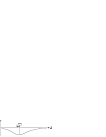
Figure 5.7: The one-loop potential is a continuous negative function with a global minimum for $R_{i}=\sqrt{\alpha^{\prime}}$.

————————————————————————————————————–

Chapter 6 Genus-One Amplitudes for intersecting Branes

In this chapter we will discuss some of the main features of toroidal compactifications with intersecting branes [108]. This quite interesting class of string backgrounds lead to four-dimensional chiral spectra, and eventually offer diverse mechanisms for breaking supersymmetry [109, 110, 111]. They have been object of intense investigation in orientifold constructions [120, 121, 122, 123, 124] and in its T-dual version as magnetic backgrounds [110, 112, 113]. The aim here is to introduce the main aspects that are relevant for the discussion of the effects of the Scherk-Schwarz mechanism on D-branes at angles [6], presented in the next chapter. We will focus on the construction of one-loop amplitudes, on computations of tadpole contributions from the transverse diagrams and on the analysis of the spectra of closed and open string excitations.

Since, as we shall explain, configurations of intersecting branes on one side and magnetised D-branes on the other are connected via T-duality, in the following we will switch from one picture to the other following our convenience.

6.1 World-Sheet Action and Boundary Conditions for Open Strings on Magnetic Backgrounds

Open strings couple in a natural way through their charged endpoints to a magnetic background $F_{ij}$ [114, 115]. The $U(1)$-invariant coupling for the bosonic part of the open string action in conformal gauge is

$$S=\frac{1}{4\pi\alpha^{\prime}}\int d\sigma d\tau\partial^{\alpha}X^{\mu}\partial_{\alpha}X_{\mu}-q_{L}\int d\tau A_{i}(X)\partial_{\tau}X^{i}(0,\tau)-q_{R}\int d\tau A_{i}(X)\partial_{\tau}X^{i}(\pi,\tau),$$ (6.1)

where $A_{i}$ is the vector potential $F_{ij}=\partial_{i}A_{j}-\partial_{j}A_{i}$.

In the simplest case of constant magnetic field along two directions $F_{ij}=F\epsilon_{ij}$ $i,j=1,2$, the open string boundary conditions for the $q_{L}$ charged left end-point are modified as follows

$$\partial_{\sigma}X^{1}(0,\tau)-2\pi\alpha^{\prime}q_{L}F\partial_{\tau}X^{2}(0,\tau) = 0,$$

$$\partial_{\tau}X^{1}(0,\tau)+2\pi\alpha^{\prime}q_{L}F\partial_{\sigma}X^{2}(0,\tau) = 0.$$ (6.2)

Similar conditions hold for the right endpoint, after the replacement $q_{L}\rightarrow-q_{R}$.

The constant $F_{ij}$ along two directions on a D-p brane thus mixes the boundary conditions for the two open-string coordinates that couple to the background.

By performing a T-duality, say along the 2-direction $X^{2}\rightarrow\tilde{X^{2}}$, one can achieve a more geometrical picture for the meaning of these boundaries conditions. T: $X^{2}\rightarrow\tilde{X^{2}}$ interchanges the two world-sheet coordinates for this direction ($\tilde{X}^{2}(\sigma,\tau)=X^{2}(\tau,\sigma))$ and thus $\partial_{\sigma}X^{2}\stackrel{{\scriptstyle T}}{{\leftrightarrow}}\partial_{\tau}\tilde{X}^{2}$ and $\partial_{\tau}X^{2}\stackrel{{\scriptstyle T}}{{\leftrightarrow}}\partial_{\sigma}\tilde{X}^{2}$, so that the boundary conditions in the T-dual picture read

$$\partial_{\sigma}\left(X^{1}(0,\tau)-2\pi\alpha^{\prime}q_{L}F\tilde{X}^{2}(0,\tau)\right) = 0$$

$$\partial_{\tau}\left(X^{1}(0,\tau)+2\pi\alpha^{\prime}q_{L}F\tilde{X}^{2}(0,\tau)\right) = 0.$$

From the conditions in (6.1) it follows that the left endpoint of the open string lives on a D-(p-1) brane, rotated by an angle $tg(\phi_{L})=-2\pi\alpha^{\prime}q_{L}F$. Similar conditions apply to the right open string endpoint which is constrained to live on a distinct D-(p-1) brane rotated by $tg(\phi_{R})=2\pi\alpha^{\prime}q_{R}F$, as far as $q_{L}\neq-q_{R}$. Therefore a neatly charged open string is effectively stretched between two D-(p-1) branes intersecting under the non trivial angle $\phi=|\phi_{L}|+|\phi_{R}|=tg^{-1}(2\pi\alpha^{\prime}q_{L}F)+tg^{-1}(2\pi\alpha^{\prime}q_{R}F)$. While if $q_{L}=-q_{R}$ the two angles coincide and thus both the endpoints live on a single rotated D-(p-1) brane, as shown in fig. 6.1 .

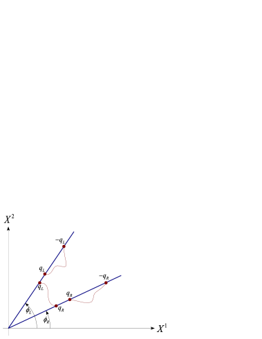
Figure 6.1: After a $T$-duality along one of the two coordinates of the two torus, magnetised D-branes become intersecting (D-1)-branes. The left endpoint of the open string lives on one of such branes, rotated by an angle $tg(\phi_{L})=-2\pi\alpha^{\prime}q_{L}F$, while the right endpoint lives on a brane rotated by $tg(\phi_{R})=2\pi\alpha^{\prime}q_{R}F$. Thus open strings with a net total charge stretch between two distinct branes, while dipole open string with $q_{L}=-q_{R}$ live on a single brane, rotated by $tg(\phi)=2\pi\alpha^{\prime}qF$.

In order to compute the spectrum of open strings on magnetised branes one needs to find the eighenfunctions of the wave operator satisfying the mixed conditions (6.2).

By using complex coordinates $X^{\pm}=\frac{1}{\sqrt{2}}\left(X^{1}\pm iX^{2}\right)$ one is able to disentangle the boundary conditions

$$\partial_{\sigma}X^{+}(0,\tau)-2i\pi\alpha^{\prime}q_{R}F\ \partial_{\tau}X^{+}(0,\tau) = 0,$$

$$\partial_{\tau}X^{+}(\pi,\tau)+2\pi\alpha^{\prime}q_{L}F\ \partial_{\sigma}X^{+}(\pi,\tau) = 0,$$ (6.4)

where $X^{-}=(X^{+})^{*}$.

The eighenfunctions of the world-sheet wave operator $\partial^{\alpha}\partial_{\alpha}$ satisfying (6.4) for a charged open string $(q_{L}+q_{R}\neq 0)$ are

$$\phi_{n}(\sigma,\tau)=\frac{1}{\sqrt{|n-\delta|}}e^{-i\tau(n-\delta)}\cos[(n-\delta)\sigma+\Phi_{L}],$$ (6.5)

$\delta=(\phi_{L}+\phi_{R})/\pi$ being the shift on the vibrational frequency depending on the angle $(\phi_{L}+\phi_{R})$ (in $\pi$ unites) between the two branes.

The solution for a charged classical vibrating string $q_{L}+q_{R}\neq 0$ of $(\partial^{2}_{\sigma}-\partial^{2}_{\tau})X^{+}=0$ is then a general combination of fundamental harmonics $\phi_{n}$

$$X^{+}=x^{+}+i\left(\sum_{n\geq 1}a_{n}\phi_{n}-\sum_{n\geq 0}b^{*}_{n}\phi_{-n}\right).$$ (6.6)

After canonical quantisation one finds the usual harmonic oscillator commutator relations between the operators $a_{n}$ and $b_{n}$, so that $a_{n}$ creates states whose masses are lowered by $-\delta$, while the states created by $b_{n}$ have masses shifted by $+\delta$.

Also the centre of mass operators $x^{+}$ and $x^{-}$ do not commute anymore

$$[x^{+},x^{-}]=\frac{\pi\alpha^{\prime}}{\phi_{L}+\phi_{R}}.$$ (6.7)

Since the Hamiltonian does not depend on these operators one can diagonalise at the same time the energy with say $x^{+}$, so that the spectrum is $x^{-}$ degenerate.

This is the stringy analogous of the the Landau degeneracy for a point charge in a uniform magnetic field.

Moreover, the absence of a momentum in the normal mode expansion (6.6) can be explained by the fact that in the $T$-dual picture the centre of mass of the open string is stuck at the brane intersection, with a quantum mechanical uncertainty (6.7), proportional to a string effective length.

For open dipole strings the frequencies are not shifted $\delta=(\phi_{L}+\phi_{R})/\pi=0$, but the zero modes in the coordinate expansion are modified as follows [115]

$$X^{+}=\frac{x^{+}+p_{-}(\tau-i\ tg(\Phi))(\sigma-\frac{\pi}{2})}{\sqrt{1+tg^{2}(\Phi)}}+\ldots,$$ (6.8)

the ellipsis referring to the contributions from the unshifted oscillators.

In the T-dual picture with intersecting branes on a compact space the scaling factor that appears in the zero mode in (6.8) takes simply into account the length of the rotated brane on the compact space, as we will discuss in the following.

Moving to the coupling of the world-sheet fermions to the magnetic background

$$S_{F}=\frac{i}{4\pi\alpha^{\prime}}\int d\sigma d\tau\bar{\psi}^{\mu}\gamma^{\alpha}\partial_{\alpha}\psi_{\mu}-\frac{iq_{L}}{4}\int d\tau\bar{\psi}^{\nu}(0)\gamma^{0}\psi_{\mu}(0)-\frac{iq_{R}}{4}\int d\tau\bar{\psi}^{\nu}(\pi)\gamma^{0}\psi_{\mu}(\pi),$$ (6.9)

the boundary conditions read

$$(\psi^{1}_{L}-Fq_{L}\psi^{2}_{R})\delta\psi^{1}_{L}-(\psi^{1}_{R}+Fq_{L}\psi^{2}_{L})\delta\psi^{1}_{R}$$

$$+(\psi^{2}_{L}+Fq_{L}\psi^{1}_{R})\delta\psi^{2}_{L}-(\psi^{2}_{R}-Fq_{L}\psi^{1}_{L})\delta\psi^{2}_{R}=0,$$ (6.10)

for the left charged endpoint and similarly for the right endpoint after the replacement $q_{L}\rightarrow-q_{R}$.

Notice how the magnetic background induces a mixing between $\psi^{1}$ and $\psi^{2}$ with respect to the usual boundary conditions on the type I world-sheet fermions

$$\psi^{\mu}_{L}\delta\psi^{\mu}_{L}-\psi^{\mu}_{R}\delta\psi^{\mu}_{R}=0.$$ (6.11)

In a complex basis $\psi^{\pm}=\frac{1}{\sqrt{2}}(\psi^{1}\pm i\psi^{2})$ one is able to resolve the mixing between the two coordinates

$$(1\mp iFq_{L})\psi^{\pm}_{L}(0) = (1\pm iFq_{L})\psi^{\pm}_{R}(0)$$

$$(1\pm iFq_{R})\psi^{\pm}_{L}(\pi) = (-)^{a}(1\mp iFq_{R})\psi^{+}_{R}(\pi),$$ (6.12)

where in the above equations $a=0$ for the R sector while $a=1$ for the NS one.

The eighenfunction of the two dimensional Dirac operator which solves the above boundary conditions for the R sector are

$$\psi^{R\pm}_{n}=\left(\begin{array}[]{c}\psi^{\pm}_{n,L}\\ \psi^{\pm}_{n,R}\end{array}\right)=\frac{1}{\sqrt{2}}\left(\begin{array}[]{c}e^{-[i(n\pm\delta)(\tau+\sigma)\pm\Phi_{L}]}\\ e^{-[i(n\pm\delta)(\tau-\sigma)\mp\Phi_{L}]}\end{array}\right),$$

while in the NS sector are

$$\psi^{NS\pm}_{n}=\left(\begin{array}[]{c}\psi^{\pm}_{n,L}\\ \psi^{\pm}_{n,R}\end{array}\right)=\frac{1}{\sqrt{2}}\left(\begin{array}[]{c}e^{-[i(n-\frac{1}{2}\pm\delta)(\tau+\sigma)\pm\Phi_{L}]}\\ e^{-[i(n-\frac{1}{2}\pm\delta)(\tau-\sigma)\mp\Phi_{L}]}\end{array}\right).$$

The generic solution of the equations of motion is thus given by an expansion in the normal modes eighenspinors listed above. After the canonical anticommutators are imposed on the oscillation modes, one can construct the zero mode Virasoro operator

$$L_{0}=-\sum_{\mathbb{Z}+a/2}(n-\frac{a}{2}+\delta):d_{-n}^{-}d_{n}^{+}:+\Delta(a),$$ (6.13)

with $a=0$ for the R sector while $a=\frac{1}{2}$ for the NS one.

An important quantity in order to recover the open string spectrum is the $\Delta(a)$ normal order constant that we will compute in the next section.

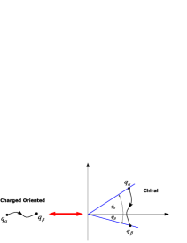
Figure 6.2:

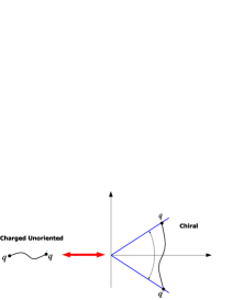
Figure 6.3:

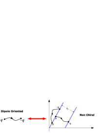
Figure 6.4:

6.1.1 Shifts on The Zero Point Energies

As shown in the previous section, both in the R and NS sectors the frequencies of the open string oscillators are shifted by the amount $\delta=\phi_{ab}/\pi$ due to the interaction with the magnetic background.

The zero point energies for the $SO(8)$ characters can be computed by regularising the divergent sums from normal ordering world-sheet modes.

For the two coordinates $X_{\pm}$ one can make the sum $\sum_{n=1}^{\infty}(n+\delta)$ to converge, by inserting a dumping factor $e^{-\epsilon(n+\delta)}$ and look at the finite $\epsilon$-independent part of the expansion

$$\sum_{n=1}^{\infty}(n+\delta)e^{-\epsilon(n+\delta)}=\frac{1}{\epsilon^{2}}-\frac{1}{12}-\frac{\delta}{2}-\frac{\delta^{2}}{2}+O(\epsilon).$$ (6.14)

Thus the vacuum shift due to $X_{\pm}$ is given by

$$\Delta_{X_{\pm}}=\frac{1}{2}\left(-\frac{2}{12}-\delta-\delta^{2}\right)=-\frac{2}{24}-\frac{\delta}{2}-\frac{\delta^{2}}{2}.$$ (6.15)

For the two world-sheet fermions in the Ramond sector, the contribution is opposite to that computed for the bosonic coordinates

$$\Delta_{\psi_{R\pm}}=+\frac{2}{24}+\frac{\delta}{2}+\frac{\delta^{2}}{2},$$ (6.16)

as one might expect by the integer-mode expansion and by world-sheet supersymmetry.

The NS contribution instead gives

$$\Delta_{\psi_{NS\pm}}=-\frac{2}{48}+\frac{\delta^{2}}{2}.$$ (6.17)

Taking into account both the shifts in the masses and in the zero point energies we can compute the characters for open strings living on the constant magnetic background

$$tr_{X_{\pm}}q^{L_{0}} = q^{-\left(\frac{2}{24}-\frac{\delta}{2}-\frac{\delta^{2}}{2}\right)}\cdot\frac{1}{\prod^{\infty}_{n=1}(1-q^{n-\delta})(1-q^{n+\delta-1})},$$

$$tr_{\psi_{R}\pm}\left(\mathcal{P}^{\pm}_{GSO}q^{L_{0}}\right) = 2q^{+\left(\frac{2}{24}+\frac{\delta}{2}+\frac{\delta^{2}}{2}\right)}\cdot\frac{\prod^{\infty}_{n=1}\left((1+q^{n-\delta})(1+q^{n+\delta-1})\pm(1-q^{n-\delta})(1-q^{n+\delta-1})\right)}{2},$$

$$tr_{\psi_{NS}\pm}\left(\mathcal{P}^{\pm}_{GSO}q^{L_{0}}\right) = q^{-\left(\frac{2}{48}-\frac{\delta^{2}}{2}\right)}\cdot\frac{\prod^{\infty}_{n=1}\left((1+q^{n-\frac{1}{2}-\delta})(1+q^{n-\frac{1}{2}+\delta})\pm(1+q^{n-\frac{1}{2}-\delta})(1+q^{n-\frac{1}{2}+\delta})\right)}{2}.$$

The different choices of GSO projections in eq. (LABEL:magchar) give the $SO(2)$ characters that encode the effects induced by the constant magnetic background on the spectrum

$$O_{2}(\delta) = tr_{\psi_{NS}\pm}\left(\mathcal{P}^{+}_{GSO}q^{L_{0}}\right),\qquad V_{2}(\delta)=tr_{\psi_{NS}\pm}\left(\mathcal{P}^{-}_{GSO}q^{L_{0}}\right),$$

$$C_{2}(\delta) = tr_{\psi_{R}\pm}\left(\mathcal{P}^{+}_{GSO}q^{L_{0}}\right),\qquad S_{2}(\delta)=tr_{\psi_{R}\pm}\left(\mathcal{P}^{-}_{GSO}q^{L_{0}}\right).$$

These characters can also be written in terms of Jacobi theta functions

$$O_{2}(\delta) = q^{\frac{\delta^{2}}{2}}\frac{\theta_{3}(\delta\tau|\tau)+\theta_{4}(\delta\tau|\tau)}{2\eta},\qquad V_{2}(\delta)=q^{\frac{\delta^{2}}{2}}\frac{\theta_{3}(\delta\tau|\tau)-\theta_{4}(\delta\tau|\tau)}{2\eta},$$

$$C_{2}(\delta) = q^{\frac{\delta^{2}}{2}}\frac{\theta_{2}(\delta\tau|\tau)-i\theta_{1}(\delta\tau|\tau)}{2\eta},\qquad S_{2}(\delta)=q^{\frac{\delta^{2}}{2}}\frac{\theta_{2}(\delta\tau|\tau)+i\theta_{1}(\delta\tau|\tau)}{2\eta},$$ (6.19)

while the contributions from the two bosonic coordinates coupled to the magnetic background is given by

$$\chi(\delta)=\frac{i\eta}{q^{\frac{\delta^{2}}{2}}\theta_{1}(\delta\tau|\tau)}.$$ (6.20)

6.2 A first Look at the Spectrum at Branes Intersections

In this section we want to give a first look at the spectrum of open strings living at the intersection of two D1-branes forming an angle $\phi_{ab}=\pi\delta$ ($|\delta|<1$), as in fig. (6.5).

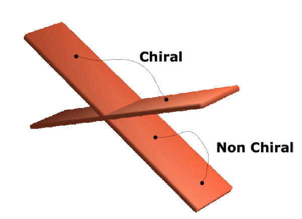
Figure 6.5: .

To this end, we decompose the ten-dimensional characters according to the breaking of the ten dimensional Lorentz group $SO(1,9)\rightarrow SO(1,7)\times SO(2)$

$$(V_{8}(\delta)-S_{8}(\delta))\chi(\delta)=\left(V_{6}(0)O_{2}(\delta)+O_{6}(0)V_{2}(\delta)-S_{6}(0)S_{2}(\delta)-C_{6}(0)C_{2}(\delta)\right)\chi(\delta),$$ (6.21)

where the internal characters are given in (6.19) and (6.20).

The essential features of the open-string spectra are that states with opposite internal helicity couple differently to the magnetic background. Their modes are shifted in opposite ways and, thus at the intersecting points only one chirality remains massless, while states of opposite chirality acquire a mass.

In particular, this is the case for compactifications to four dimensions, being one of the interesting feature of the open string spectra from intersecting branes configurations.

The spectrum at the brane intersection is encoded in the decompositions of the characters given in eq. (6.21).

The eight dimensional vector becomes massive, since $V_{6}(0)O_{2}(\delta)\chi(\delta)\sim 6q^{\delta/2}$, while $O_{6}(0)V_{2}(\delta)\chi(\delta)\sim q^{-\mid\delta\mid+\frac{\mid\delta\mid}{2}}$, the lowest scalar state is thus tachyonic.

Its presence signals the instability of the configuration of the two intersecting branes that break all the supersymmetries. In fact the two branes are each separately 1/2 BPS but for a generic intersection angle they preserve two different combinations of supercharges, thus breaking all the original type II supersymmetries.

In this situation there is not a cancellation between gravitational attraction and RR repulsion between the two branes and the system is not a true vacuum, where quantum fluctuations might be considered under control. Indeed tree-level exchanges of closed states will certainly drive the system to a new configuration, maybe through brane recombination where, after a tachyon condensation process [116], the system can reach a nearby true vacuum.

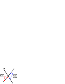
Figure 6.6: .

However, when the two branes intersects on a higher dimensional torus $T^{d}$, for $d\geq 4$, particular configurations of intersecting branes exist where some amount of the original supersymmetry is preserved and the scalar excitations return to be massless, being part of a matter supermultiplet.

The ten-dimensional character $S_{8}$ decomposes into the sum of two eight dimensional characters with opposite chirality ($S_{6}$), ($C_{6}$).

Due to the magnetic background, the states in one of the two eight-dimensional characters become all massive, while those in the other one remain massless. Which of the two internal helicity characters acquires a mass depends on the sign of the relative angle between the two D-branes. This can be clearly seen by the leading term expansions for the internal characters

$$C_{6}(0)S_{2}(\delta)\chi(\delta)\sim q^{-\frac{\delta}{2}+\frac{\mid\delta\mid}{2}}\qquad S_{6}(0)C_{2}(\delta)\chi(\delta)\sim q^{\frac{\delta}{2}+\frac{\mid\delta\mid}{2}}.$$ (6.22)

Therefore the character that contains massless states supplies half of the degree of freedom of an eight dimensional Weyl spinor. The remaining half is given by the mirror sector, open strings with left end right endpoints interchanged that experience an opposite shift $-\delta$ in their mode expansion. The presence of a mirror sector is due to the introduction of orientifold planes, as usual necessary in order to cancel the total RR charge and get an anomaly-free massless spectrum.

Not to break translational invariance in the extended dimensions, the D-branes transverse directions need to be compact. Since the D-branes are sources of RR fluxes on their transverse directions and the flux lines cannot escape at infinity on the compact space, the presence of an opposite charged object that can sink the Faraday lines of the D-branes is necessary to avoid a violation of the equations of motion, that are a version of Gauss low for charged extended objects.

Orientifold planes in turns require the presence of mirror D-branes, whose open-string excitations have left and right endpoints interchanged with respect to the original ones. Their normal modes are therefore subjected to an opposite shift.

It turns out that in the mirror sector there are the missing degrees of freedom to form a one chirality eight-dimenisonal Weyl spinor.

Therefore at the brane intersection we have the number of degrees of freedom of an eight-dimensional Weyl spinor, accompanied by (scalar) tachyonic excitations.

6.3 Magnetised Branes Topological Invariants and Intersecting Branes Wrapping Numbers

In order to take into account all the open string sectors excitations of the magnetised branes wrapping a torus, one still need a generalisation of the Dirac quantisation condition between electric and magnetic charges. In the T-dual picture this condition translates into a statement on the geometry of the rotated-branes configurations.

Let us consider a constant magnetic field $F$ on a two torus $T^{2}$, whose coordinates on the two canonical cycles are $x\sim x+L_{1}$ and $y\sim y+L_{2}$. One can write the $U(1)$ potential locally as $A=(0,\frac{1}{2}Fx)$, but globally, in order to respect the periodicity along the two cycles, two different coordinate patches are needed.

As an example, one can take the following two regions as in fig. 6.7, $0\leq x<a$ with $A_{I}=(0,\frac{1}{2}Fx)$, and $a\leq x<L_{1}$ with $A_{II}=(0,\frac{1}{2}F(x-L_{1}))$.

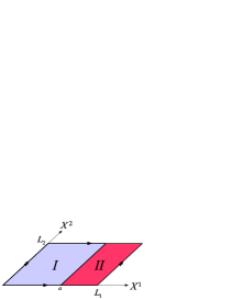
Figure 6.7:

The magnetic field on the torus is therefore a non trivial $U(1)$ gauge bundle ($F\neq 0$ in cohomology), and as a result a non vanishing magnetic field corresponds to the presence of magnetic charges, (see (2.124) and the related discussion).

The first Chern number associated to the non trivial bundle is a non vanishing integer

$$\frac{1}{4\pi^{2}}\int_{T^{2}}F=m.$$ (6.23)

For a constant magnetic field on a square $T^{2}$ the above condition gives

$$\frac{1}{4\pi^{2}}FL_{1}L_{2}=m.$$ (6.24)

If one considers a magnetised brane wrapping $n$ times the $T^{2}$ the firs Chern number needs to be modified to

$$\frac{n}{4\pi^{2}}\int_{T^{2}}F=m,$$ (6.25)

since due to the wrapping number $n$, the brane volume is $n$ times the $T^{2}$ volume.

A T-duality along the $y$ direction $L_{2}\rightarrow\alpha^{\prime}/L_{2}$ transforms the magnetised D-p brane into a D-(p-1)brane rotated by an angle $tg\phi=2\pi\alpha^{\prime}F$, and the relation (6.25) into

$$tg\phi=\frac{m}{n}\frac{L_{2}}{L_{1}},$$ (6.26)

which shows that the integer $m$ corresponds to the number of times the brane wraps around the vertical cycle, while $n$ corresponds the the horizontal wrapping number [113].

6.4 One-Loop Amplitudes for Intersecting Branes Wrapping a Two Torus

We consider the configuration of intersecting branes wrapping a two-torus $T^{2}$ shown in fig. 6.8.

An O8 plane wraps one of the two homology cycles, while a stack $N_{\alpha}$ and its orientifold image $\bar{N}_{\alpha}$ form an angle $\phi_{\alpha}$ (respectively $-\phi_{\alpha}$) with the $O8$-plane.

The presence of the O8 plane, necessary to cancel the total RR charge, induces a $\Omega I$ symmetry on both the closed and open string spectrum, $I$ being a reflection along $X^{2}$, the orthogonal direction to the O-plane and $\Omega$ the world-sheet parity.

The $I$ reflection needs to act in a crystallographic way on the target two torus, it is not then difficult to see that this is the case only when the real part $U_{1}$ of the $T^{2}$ complex structure is vanishing or equals to $1/2$.

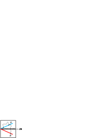
Figure 6.8: A portion of a stack of $N$ branes is represented in blue, while in red is represented its image under the mirror orientifold plane (horizontal wavy line).

Therefore the off-diagonals entries of the metric in the canonical homology basis, given by $U_{1}$ in eq.(5.129), in the presence of the O8-plane become discrete moduli with the possible values $U_{1}=0,1/2$. This is the T-dual manifestation of what we have already encountered for the $B_{ij}$ field in the presence of O7 planes as discussed in sec. 4.6. In fact, after a T-duality along one of the two internal coordinates, the dimensions of the D-branes and O-planes are increased or lowered, depending whether the duality is along directions orthogonal or parallel to these objects. The $T^{2}$ complex structure $U$ and the Khäler class $T$ get also interchanged and, in particular, $b$ plays the role here played by $U_{1}$. At the moment we consider the case $U_{1}=0$, corresponding to a square $T^{2}$, we will consider in the next chapter also the case of a $U_{1}=1/2$ tilted target torus, which however presents only few slightly differences.

The closed string spectrum for the background we are considering is encoded in the one-loop amplitudes $\frac{1}{2}\mathcal{T}+\mathcal{K}$

$$\mathcal{T} = (V_{8}-S_{8})(\bar{V_{8}}-\bar{C_{8}})\Lambda_{\vec{m}\vec{n}},$$

$$\mathcal{K} = \frac{1}{2}(V_{8}-S_{8})P_{\vec{m}}W_{\vec{n}}.$$ (6.27)

A change of proper time in the second of eqs. (6.27) gives the transverse Klein bottle amplitude $\tilde{\mathcal{K}}$, proportional to the square of the tension and the charge of the $O8$ plane

$$\tilde{\mathcal{K}}=\left(2^{2}\ \sqrt{\frac{L_{1}}{L_{2}}}\right)^{2}(V_{8}-S_{8})W_{\vec{2n}}P_{\vec{2m}}.$$ (6.28)

Turning to the open string amplitudes, the brane excitations are encoded in $\mathcal{A}$ and $\mathcal{M}$.

The Annulus is given by

$$\mathcal{A} =N_{\alpha}\bar{N}_{\alpha}(V_{8}-S_{8})(0)P_{m}(L_{||})W_{n}(L_{\perp})$$ (6.29)

$$+ \left(\frac{N_{\alpha}^{2}}{2}(V_{8}-S_{8})\left(2\Phi_{\alpha}\tau/\pi\right)+\frac{\bar{N}_{\alpha}^{2}}{2}(V_{8}-S_{8})\left(2\Phi_{\alpha}\tau/\pi\right)\right)\frac{2k_{\alpha}\omega_{\alpha}\cdot i\eta}{\theta_{1}\left(2\Phi_{\alpha}\tau/\pi\mid\tau\right)},$$

where the first line gives the contribution from dipole string that live on rotated branes, whose Kaluza-Klein momenta are scaled by the effective length of the brane $L_{||}$, and winding are possible between parallel wrappings of the branes, $L_{\perp}$ being the minimal distance between two consecutive D-brane wrapping , (see fig. 6.9).

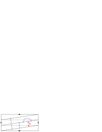
Figure 6.9: Open strings living on a rotated brane wrapping the $T^{2}$. The Kaluza-Klein momenta are proportional to $1/L_{||}$, where $L_{||}$ is the length of the brane, while the windings are multiple of $L_{\perp}$, the minimal distance between two consecutive wrappings of the brane on the $T^{2}$.

In the second line of (6.29) is displayed the contribution from the unoriented charged open strings and their image under the mirror O8 plane. In this sector open strings stretch between branes and their orientifold images.

The multiplicity factor $2\kappa_{\alpha}\omega_{\alpha}$ is the intersection number $I_{\alpha\bar{\alpha}}$ , that corresponds to the number of intersections between the brane and its image. Due to the possibility of multiple intersections of two lines on a compact space, replicas of chiral matter sectors emerge naturally from intersecting branes configurations.

In the Möbius only the unoriented states in the last two terms of (6.29) can flow

$$\mathcal{M}=-\left(\frac{N_{\alpha}}{2}(\hat{V}_{8}-\hat{S}_{8})\left(2\Phi_{\alpha}\tau/\pi\right)+\frac{\bar{N}_{\alpha}}{2}(\hat{V}_{8}-\hat{S}_{8})\left(2\Phi_{\alpha}\tau/\pi\right)\right)\frac{2k_{\alpha}\cdot i\hat{\eta}}{\hat{\theta}_{1}\left(2\Phi_{\alpha}\tau/\pi\mid\tau\right)}.$$ (6.35)

Notice the multiplicity factor $2k_{\alpha}$, corresponding to the number of intersection points between the brane and its image that belong also to the pair of O-8 planes, the two fixed circles $y=0$ and $y=L_{2}/2$ under the involution $I$, (see fig. 6.10).

The gauge sector is given by the massless excitations of the oriented dipole strings in the annulus amplitude, the first term in (6.29). After a dimensional reduction of the original SO(8) characters we have

$$\mathcal{A}^{Or}_{0}=N_{\alpha}\bar{N}_{\alpha}(V_{6}O_{2}(0)+O_{6}V_{2}(0)-S_{6}C_{2}(0)-C_{6}S_{2}(0)),$$ (6.36)

where the multiplicity $N_{\alpha}\bar{N}_{\alpha}$ in front of $V_{8}$ corresponds to the dimension of the adjoint representation of the unitary group $U(N_{\alpha})$.

The reason why the gauge group is unitary follows from the fact that the vectors and the gauginos correspond to oriented dipole string excitations that cannot flow in the Möbius. Only in the limit of uncharged open strings, corresponding to a vanishing angle between the stacks of branes and the O-plane, these states become unoriented and one recovers the previously discussed configurations of D-branes on top of O-planes, with $SO(N)$ or $USp(2M)$ gauge groups.

From eq. (6.36) one can read the physical degrees of freedom of an eight-dimensional gauge boson vector, contained in $V_{6}O_{2}(0)$, two massless scalars from $O_{6}V_{2}(0)$ and two opposite chirality gauginos from $S_{6}C_{2}(0)$ and $C_{6}S_{2}(0)$. Altogether, these massless excitations correspond to a $\mathcal{N}=1$ $d=8$ super Yang Mills $U(N_{\alpha})$ vector multiplet.

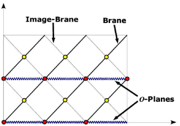
Figure 6.10: Multiple intersections between a brane and its image with respect an orientifold plane. If the brane has integer wrapping numbers $(\omega,\kappa)$ and its image $(\omega,-\kappa)$, the total number of intersections is given by $2\omega\kappa$. $2\kappa$ of such points (in red) belong also to the pair of O-planes, while the remaining $2(\omega-1)\kappa$ intersection points (in yellow) fall outside of the O-planes.

The non-supersymmetric matter lives at the intersection points between branes and image branes, and they come in a number of families which equals the intersection number. The matter states are given by fermionic massless states and tachyonic excitations. In the present case of a single stack $N_{\alpha}$ and its orientifold image $\bar{N}_{\alpha}$, the open string stretching between those objects have equal charge at their endpoints and thus are unoriented. These states are given by the last two terms in the Annulus (6.29) and are the only contributions to the Möbius amplitude (6.35)

$$\mathcal{A}^{Un}_{0}+\mathcal{M}_{0}=$$

$$\left[\left(\frac{N_{\alpha}^{2}}{2}-\frac{N_{\alpha}}{2}\right)\frac{2\omega_{\alpha}k_{\alpha}+2k_{\alpha}}{2}+\left(\frac{N_{\alpha}^{2}}{2}+\frac{N_{\alpha}}{2}\right)\frac{2\omega_{\alpha}k_{\alpha}-2k_{\alpha}}{2}\right]\left(O_{6}V_{2}(2\phi_{\alpha})-C_{6}S_{2}(2\phi_{\alpha})\right)$$

$$+ \left[\left(\frac{\bar{N}_{\alpha}^{2}}{2}-\frac{\bar{N}_{\alpha}}{2}\right)\frac{2\omega_{\alpha}k_{\alpha}+2k_{\alpha}}{2}+\left(\frac{\bar{N}_{\alpha}^{2}}{2}+\frac{\bar{N}_{\alpha}}{2}\right)\frac{2\omega_{\alpha}k_{\alpha}-2k_{\alpha}}{2}\right]\left(O_{6}V_{2}(-2\phi_{\alpha})-S_{6}C_{2}(-2\phi_{\alpha})\right).$$

From the above amplitudes one can read $2\omega_{\alpha}k_{\alpha}$ families of chiral spinors and (tachyonic) scalars, each for every intersection between the brane and its orientifold image.

$A_{\alpha}=(2\omega_{\alpha}k_{\alpha}+2k_{\alpha})/2$ of these families carry an antisymmetric representation of the gauge group $U(N_{\alpha})$, (see fig. 6.10 ).

Whenever a stack $N_{\alpha}$ wraps more than one time the horizontal one-cycle ($\omega_{\alpha}>1$), a number given by $S_{\alpha}=(2\omega_{\alpha}k_{\alpha}-2k_{\alpha})/2$ of intersection points of the total $2\omega_{\alpha}k_{\alpha}$ fall outside the orientifold planes and $S_{\alpha}$ families carry a symmetric representation of the $U(N_{\alpha})$ gauge group.

In a more general situation, where more than one rotated stack are present, the open strings stretching between two different stacks $N_{\alpha}$ and $N_{\beta}$ have different charge at their endpoints and therefore are oriented. These states cannot flow in the Möbius, thus come in bifundamental representations of the gauge group $U(N_{\alpha})\times U(N_{\beta})$.

The presence of tachyonic excitations at the intersection points signals the instability of the configuration that breaks all the supersymmetries.

To compute the fate of the final configuration is in general quite problematic in string theory due to the dificulties connected to the issues of background redefinition in a first quantised formulation. Nonetheless, various old and new suggestions have been given to these problems [55, 56, 117]. At the end of the day tachyonic excitations might be very welcome, since they could trigger gauge symmetry breaking through a process of tachyon condensation which also induces brane recombination processes.

6.5 Tadpole cancellation conditions

In order to compute the various tadpole contributions one needs to extract the coefficients in front of the closed string massless states flowing in the cylinder, Klein bottle and Möbius strip tree-level diagrams.

The characters in the presence of the magnetic background have been written in terms of Jacobi theta function in (6.19), therefore to go to the transverse channel one can use the well known behaviour of the theta functions under an S modular transformation

$$\theta\left[{}^{\alpha}_{\beta}\right]\left(\frac{\zeta}{\tau}|-\frac{1}{\tau}\right)=(-i\tau)^{\frac{1}{2}}e^{2\pi\alpha\beta}e^{i\pi\frac{\zeta^{2}}{\tau}}\theta\left[{}^{-\beta}_{\alpha}\right](\zeta|\tau).$$ (6.37)

From the one loop Annulus amplitude (6.29), and with the help of the previous relation, one can compute the transverse Annulus amplitude

$$\tilde{\mathcal{A}} = 2^{-5}\left(\frac{L_{||}}{L_{\perp}}N_{\alpha}\bar{N}_{\alpha}(V_{8}-S_{8})W_{n}(L_{\perp})P_{m}(L_{||})\right)$$ (6.38)

$$+ 2^{-4}\left(\frac{N_{\alpha}^{2}}{2}(V_{8}-S_{8})(2\phi_{\alpha}/\pi|l)+\frac{\bar{N}_{\alpha}^{2}}{2}(V_{8}-S_{8})(-2\phi_{\alpha}/\pi|l)\right)\frac{2k_{\alpha}\omega_{\alpha}\eta}{\theta_{1}(2\phi_{\alpha}/\pi|l)}.$$

From the expressions for the theta functions one can obtain the leading terms in the expansions of the closed string characters

$$O_{2}(\phi/\pi|l) \sim 1\qquad V_{2}(\phi/\pi|l)\sim\cos(\phi)$$

$$C_{2}(\phi/\pi|l) \sim e^{-i\frac{\phi}{2}}\qquad S_{2}(\phi/\pi|l)\sim e^{i\frac{\phi}{2}},$$ (6.39)

and

$$\theta_{1}(\phi/\pi|l)\sim 2sin(\phi).$$ (6.40)

These leading terms in (6.39) and (6.40) are the ingredients that one needs in order to extract the tadpole contributions from the various diagrams.

Since closed-string modes are not shifted by the magnetic field, the effects of the $U(1)$ background enter only in modifying the reflection coefficients in the transverse amplitudes. In particular for this reason one does not need to care about zero point energy shifts in the closed string characters, since they cancel each-other as in the standard (unmagnetised) case.

The Annulus amplitude contribution to the NSNS tadpole is given by the coefficient in front of the NSNS massless states, contained in the character $V_{6}$ in (6.38)

$$V_{8}(2\phi_{\alpha}/\pi|l)=V_{6}(0|l)O_{2}(2\phi_{\alpha}/\pi|l)+O_{6}(0|l)V_{2}(2\phi_{\alpha}/\pi|l).$$ (6.41)

It corresponds to $\mathcal{B}^{2}$, the square of the one point function for the emission of the dilaton $\phi$ or $g_{\mu}^{\mu}$ from a disk.  By using the (6.39) and (6.40) one then obtains

$$\mathcal{B}^{2}=2^{-5}\left[\frac{L_{||}}{L_{\perp}}N_{\alpha}\bar{N}_{\alpha}+\left(\frac{N_{\alpha}^{2}}{2}+\frac{\bar{N}_{\alpha}^{2}}{2}\right)\frac{k_{\alpha}\omega_{\alpha}}{sin\phi_{\alpha}\cos\phi_{\phi_{\alpha}}}\right].$$ (6.42)

As expected, the above expression can be written as e perfect square by using the relation between the lengths $L_{||}$ and $L_{\perp}$ and the angle $\phi_{\alpha}$.

$$\mathcal{B}^{2}=\left(2^{-3}\sqrt{\frac{L_{||}}{L_{\perp}}}(N_{\alpha}+\bar{N}_{\alpha})\right)^{2}.$$ (6.43)

The transverse Möbius amplitude is given by

$$\tilde{\mathcal{M}}=-\left(\frac{N_{\alpha}}{2}(\hat{V}_{8}-\hat{S}_{8})(\phi_{\alpha}/\pi|l)+\frac{\bar{N}_{\alpha}}{2}(\hat{V}_{8}-\hat{S}_{8})(-\phi_{\alpha}/\pi|l)\right)\frac{2k_{\alpha}\hat{\eta}}{\hat{\theta}_{1}(2\phi_{\alpha}/\pi|l)},$$ (6.44)

where to lighten the notation in the above expression, we did not explicitly write the real part of the Möbius proper time .

The contribution from this diagram to the NSNS tadpole is therefore

$$\tilde{\mathcal{M}}=-2(N_{\alpha}+\bar{N}_{\alpha})\frac{L_{||}}{L_{2}}$$ (6.45)

that is consistently equal to $-2\sqrt{\mathcal{B}^{2}\cdot\mathcal{C}^{2}}$, twice the square-root of the product between the amplitude $\mathcal{B}$ for the emission of massless states from an O-plane $\mathcal{C}$ and those from a D-brane (6.42).

The total NSNS tadpole contributions from the transverse diagrams reads

$$\tilde{\mathcal{K}}_{0}+\tilde{\mathcal{A}}_{0}+\tilde{\mathcal{M}}_{0} = \mathcal{C}^{2}+\mathcal{B}^{2}-2\mathcal{C}\mathcal{B}=\left(\mathcal{B}-\mathcal{C}\right)^{2}$$

$$= \left(2^{-3}\sqrt{\frac{L_{||}}{L_{\perp}}}(N_{\alpha}+\bar{N}_{\alpha})-2^{2}\sqrt{\frac{L_{1}}{L_{2}}}\right)^{2}.$$

NSNS tadpole cancellation condition therefore asks for

$$\sqrt{\frac{L_{||}}{L_{\perp}}}(N_{\alpha}+\bar{N}_{\alpha})=2^{5}\sqrt{\frac{L_{1}}{L_{2}}},$$ (6.46)

that, with the help of the relations between the effective length of the brane and the angle eq. (6.46), can be rewritten as

$$\omega_{\alpha}(N_{\alpha}+\bar{N}_{\alpha})\sqrt{1+tg(\phi_{a})^{2}}=2^{5}.$$ (6.47)

In the present case of a $T^{2}$ compactification there is not a way to cancel the NSNS tadpole (6.47) for a non vanishing angle $\phi_{\alpha}\neq 0$, and thus the configuration breaks all the supersymmetries. However, this is not the case starting for an higher dimensional $T^{d}$ compactifications for $d\geq 4$, where both BPS and not BPS configurations of intersecting branes do exist that cancel the NSNS tadpole.

After a T-duality along the vertical coordinate of the two torus, the l.h.s. of eq. (6.47), corresponds to the Dirac Born Infeld action [118, 114] for a stack $N_{\alpha}$ of magnetised D9-branes wrapping $\omega_{\alpha}$ times the two torus

$$\omega_{\alpha}(N_{\alpha}+\bar{N}_{\alpha})\sqrt{det(\,\raisebox{1.4pt}{{\hbox{{\rm\scriptsize]}} \raisebox{-1.99997pt}{\kern-8.00003pt\hbox{1}}}}\,+\mathcal{F})}=2\times 2^{4}.$$ (6.48)

This relation of course corresponds again to a condition for the cancellation between the tension of the stack of magnetised branes and the tension of the O9 planes, equal to $16$ for each of the two planes, $tg(\phi_{a})=2\pi\alpha^{\prime}\mathcal{F}$, $\mathcal{F}$ being the value of the constant magnetic field on the two-cycle

$$\mathcal{F}=2\pi\alpha^{\prime}\left(\begin{array}[]{cc}0&F\\ -F&0\end{array}\right).$$

Turning to the RR tadpole, one needs to take into account the contributions from the decomposition of the RR ten dimensional characters in $\tilde{\mathcal{A}}$ and $\tilde{\mathcal{M}}$

$$S_{8}(2\phi_{a}/\pi|l)=S_{6}(0|l)C_{2}(2\phi_{a}/\pi|l)+S_{6}(0|l)C_{2}(2\phi_{a}/\pi|l).$$ (6.49)

By using the $q$-expansions in (6.39) and (6.40), it is clear that different internal helicities

will introduce different phases in their couplings to the magnetic background.

The massless state from $S_{6}$ in $\tilde{\mathcal{A}}$ gives the following contribution

$$\mathcal{B}^{2}_{S_{6}}=2^{-6}\frac{L_{||}}{L_{\perp}}\left(N_{\alpha}e^{-i\phi_{\alpha}}+\bar{N}_{\alpha}e^{i\phi_{\alpha}}\right)^{2},$$ (6.50)

while the contribution from $C_{6}$ is

$$\mathcal{B}^{2}_{C_{6}}=2^{-6}\frac{L_{||}}{L_{\perp}}\left(N_{\alpha}e^{i\phi_{\alpha}}+\bar{N}_{\alpha}e^{-i\phi_{\alpha}}\right)^{2}$$ (6.51)

Both the contributions can be expressed by a single formula

$$\mathcal{B}^{2}_{RR}=2^{-6}\frac{L_{||}}{L_{\perp}}\left(N_{\alpha}e^{2i\phi_{\alpha}\lambda}+\bar{N}_{\alpha}e^{-2i\phi_{\alpha}\lambda}\right)^{2}$$ (6.52)

where $\lambda=\pm\frac{1}{2}$ is the helicity of the internal character (in the open string sense), that couples in different ways to the magnetic background. This formula generalises nicely to higher-dimensional (factorised) torus compactifications as we will see in the next chapter.

Taking also into account the contributions from the Klein bottle and the Möbius amplitudes, the RR tadpole cancellation condition reads

$$\sqrt{\frac{L_{||}}{L_{\perp}}}\left(N_{\alpha}e^{2i\phi_{\alpha}\lambda}+\bar{N}_{\alpha}e^{-2i\phi_{\alpha}\lambda}\right)=2^{5}\sqrt{\frac{L_{1}}{L_{2}}}.$$ (6.53)

The real part of the above equation gives

$$\omega_{\alpha}\left(N_{\alpha}+\bar{N}_{\alpha}\right)=2^{5},$$ (6.54)

while the imaginary part just asks for an equal number of branes and image branes

$$N_{\alpha}-\bar{N}_{\alpha}=0.$$ (6.55)

After having imposed this last condition eq. (6.54) asks for a cancellation between the RR charge of the stack of branes and the RR of orientifold plane

$$\omega_{\alpha}N_{\alpha}=16.$$ (6.56)

It is worth to notice that an horizontal wrapping $\omega_{\alpha}>1$ for the D8 stack increases its effective charge by $\omega_{\alpha}$ times its original value. This has a simple explanation after a T-duality along the vertical coordinate of the two torus, where the D8 branes gets mapped into $\omega_{\alpha}$ copies of D9 branes or, equivalently, to a D9 wrapping $\omega_{\alpha}$-times the two torus.

————————————————————————————————————–

Chapter 7 Scherk-Schwarz Breaking and Intersecting Branes

In this chapter we analyse the effects of the Scherk-Schwarz mechanism on configurations of intersecting branes [6]. After a discussion on the conditions under which a D-brane wrapping a torus feels the breaking or remains supersymmetric, we will show how the Scherk-Schwarz mechanism can be successfully employed to give a tree-level mass to non-chiral fermionic excitations.

This offers a solution for a longstanding problem of intersecting branes vacua since non-chiral massless fermions, ubiquitous in open string spectra of intersecting branes, are certainly not present in the standard model.

Finally, we will describe the effects of the Scherk-Schwarz mechanism on $D-7$ intersecting branes wrapping a $T^{4}$.

7.1 Scherk-Schwarz and M-theory breaking

In the following we shall review the main features of type IIB orientifolds with supersymmetry broken via momentum or winding deformations. Actually, to emphasise the geometry of these orientifolds, we focus on the more conventional momentum-deformed closed-string spectrum and study the $\Omega$ and $\Omega I$ orientifolds, where $\Omega$ is the world-sheet parity and $I$ is an inversion of the compact coordinate. The latter orientifold better described within type IIA is the T-dual description of type IIB with winding shifts.

The deformed nine-dimensional spectrum of the closed IIA and IIB oriented strings is encoded in the one-loop partition function

$$\mathcal{T} = {\textstyle{1\over 2}}\biggl{[}|V_{8}-S_{8}|^{2}\,\Lambda_{m,n}+|V_{8}+S_{8}|^{2}\,(-1)^{m}\,\Lambda_{m,n}$$ (7.1)

$$+ |O_{8}-C_{8}|^{2}\,\Lambda_{m,n+{1\over 2}}+|O_{8}+C_{8}|^{2}\,(-1)^{m}\,\Lambda_{m,n+{1\over 2}}\biggr{]}$$

where $\Lambda_{m,n}$ is a $(1,1)$-dimensional Narain lattice. Indeed, all the fermions have acquired a mass proportional to the inverse radius, and a twisted tachyon is present if $R<2\sqrt{\alpha^{\prime}}$.

The Klein bottle amplitudes associated to the two orientifolds $\Omega$ and $\Omega^{\prime}=\Omega I$ can be straightforwardly determined from 7.1 and read

$$\mathcal{K}={\textstyle{1\over 2}}\,(V_{8}-S_{8})\,P_{2m}\,,$$

and

$$\mathcal{K}\,\,^{\prime}={\textstyle{1\over 2}}\,(V_{8}-S_{8})\,W_{n}+{\textstyle{1\over 2}}\,(O_{8}-C_{8})\,W_{n+{1\over 2}}\,.$$

The former amplitude clearly spells out the presence of O9 planes while the latter involves conjugate pairs of O8 and $\overline{{\rm O}8}$ planes sitting at the two edges of the segment $S^{1}/I$.

More interesting is the open-string spectrum associated to these orientifolds. In the first case, it consists of open strings stretched between D9 branes. In particular, these branes wrap the compact direction and thus their excitations are affected by the Scherk-Schwarz deformation. Indeed, the corresponding annulus and Möbius-strip amplitudes

$$\mathcal{A}={\textstyle{1\over 2}}\,N^{2}\,\left(V_{8}\,P_{2m}-S_{8}\,P_{2m+1}\right)\,,$$

and

$$\mathcal{M}=-{\textstyle{1\over 2}}\,N\,\left(\hat{V}_{8}\,P_{2m}-\hat{S}_{8}\,P_{2m+1}\right)\,,$$

clearly reveal that the fermions are now massive and supersymmetry is spontaneously broken. In the second case, the D8 branes are transverse to the compact direction along which the Scherk-Schwarz deformation takes place, and thus the open-string spectrum is unaffected. However, the brane configuration has to respect the symmetries we are gauging, and therefore the pairs of image (anti-)branes have to be displaced at points diametrically opposite. In equations

$$\mathcal{A}\,\,^{\prime}=\left[{\textstyle{1\over 2}}\left(N^{2}+M^{2}\right)\,(V_{8}-S_{8})+M\,N\,(O_{8}-C_{8})\right]\left(W_{n}+W_{n+{1\over 2}}\right)\,,$$

and

$$\mathcal{M}\,\,^{\prime}=-{\textstyle{1\over 2}}\,(N+M)\,\hat{V}_{8}\,\left(W_{n}+W_{n+{1\over 2}}\right)+{\textstyle{1\over 2}}\,(N-M)\,\hat{S}_{8}\,\left(W_{n}-W_{n+{1\over 2}}\right)\,.$$

As expected the fermions are still massless (at tree level), while supersymmetry is broken only by the simultaneous presence of branes and anti-branes.

In conclusion, we can summarise our results as follows [93]: if the Scherk-Schwarz deformation connects points on the brane then supersymmetry is broken in the open-string sector, otherwise image branes have to be properly added in order to respect the gauged symmetry and the fermions stay massless.

7.2 Wilson lines on magnetised branes

In this section we review some known facts about magnetised (or intersecting) branes [120, 121, 122, 123, 124] and comment on the role of Wilson lines and/or brane displacements. This will give us the opportunity to present our notation and introduce some simple deformations that however will play an important role in the forthcoming sections.

7.2.1 Preliminaries on intersecting branes: notation and conventions

Let us focus our attention on the simple case of eight-dimensional reductions with D8 branes extending along one generic direction of the $T^{2}$. Lower-dimensional reductions are quite simple to study, and will be discussed in the following sections. For simplicity, we take the torus to be rectangular with horizontal and vertical sides of length $R_{1}$ and $R_{2}$, respectively. Each set of parallel branes is then identified by the pair of integers $(q,k)$ that correspond to the number of times the branes wrap the horizontal and vertical sides of the $T^{2}$, the two canonical one-cycles. In turn, these numbers determine the oriented angle $\phi$ between the horizontal axis of the torus and the brane itself via the relation

$$\tan\phi={kR_{2}\over qR_{1}}\,,$$ (7.2)

and it is positive (negative) if starting from the horizontal axis we move counter-clock-wise (clock-wise) towards the brane. By simple trigonometry arguments, we can then determine the effective length of the brane

$$L_{\|}=\sqrt{(qR_{1})^{2}+(kR_{2})^{2}}\,,$$

and the distance between consecutive wrappings on the $T^{2}$

$$L_{\perp}={R_{1}R_{2}\over L_{\|}}\,.$$

Using the quantisation condition (7.2), $L_{\|}$ and $L_{\perp}$ can be conveniently written as

$$L_{\|}={qR_{1}\over\cos\phi}={kR_{2}\over\sin\phi}\,,\qquad\quad L_{\perp}={R_{2}\over q}\cos\phi={R_{1}\over k}\sin\phi\,.$$

Given these two quantities it is then easy to determine the zero-mode spectrum of open strings stretched on this rotated brane [110, 120, 121, 122, 123, 124]

$$M^{2}_{\rm z.m.}=\left({m\over L_{\|}}\right)^{2}+{1\over\alpha^{\prime}{}^{2}}\left(nL_{\perp}\right)^{2}\,.$$

It simply consists of Kaluza-Klein states along the compact direction of the brane and of winding states between two portions of the brane in the elementary cell of the $T^{2}$, as indicated in figure 7.1.

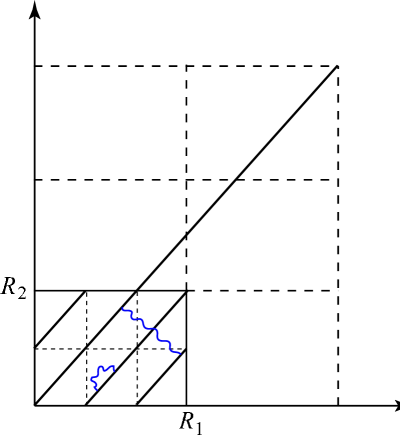
Figure 7.1: Zero-mode spectrum on a rotated brane with wrapping numbers $(2,3)$.

If orientifold planes and/or other branes are present, one has to consider new sectors corresponding to open-strings stretched between two different branes. These new sectors are particularly appealing since they typically support chiral matter at the intersection loci, while the masses of the string excitations now depend on the relative angle $\phi_{\alpha}-\phi_{\beta}$, and the precise dependence changes in the NS and R sectors.

As usual, it is convenient to summarise the complete spectrum of string excitations in the annulus, and eventually Möbius-strip, partition function. To this end let us consider the simple case of an $\Omega\mathscr{R}$ orientifold, with $\Omega$ the standard world-sheet parity and $\mathscr{R}:\ z\to\bar{z}$ an anti-conformal involution acting on the complex coordinate $z\equiv y_{1}+iy_{2}$ of the $T^{2}$. This operation, a symmetry of the IIA string, introduces two pairs of horizontal O8 planes, passing through the points $y_{2}=0$ and $y_{2}={1\over 2}R_{2}$. Introducing a stuck of $N_{\alpha}$ coincident D8 branes with wrapping numbers $(q_{\alpha},k_{\alpha})$ breaks in general the orientifold symmetry, unless a suitable stack of $N_{\alpha}$ image branes with wrapping numbers $(q_{\alpha},-k_{\alpha})$ is also added [120, 121, 122, 123, 124]. The annulus amplitude then consists of different sectors corresponding to strings stretched between a pair of (image-)branes and to strings stretched between a brane and its image:

$$\mathcal{A} = N_{\alpha}\bar{N}_{\alpha}\,(V_{8}-S_{8})[{\textstyle{0\atop 0}}]\,P_{m}(L_{\|\alpha})W_{n}(L_{\perp\alpha})$$ (7.3)

$$+ {\textstyle{1\over 2}}\left(N^{2}_{\alpha}\,(V_{8}-S_{8})[{\textstyle{\alpha\bar{\alpha}\atop 0}}]+\bar{N}^{2}_{\alpha}\,(V_{8}-S_{8})[{\textstyle{\bar{\alpha}\alpha\atop 0}}]\right)\,{2q_{\alpha}k_{\alpha}\over\Upsilon_{1}[{\textstyle{\alpha\bar{\alpha}\atop 0}}]}$$

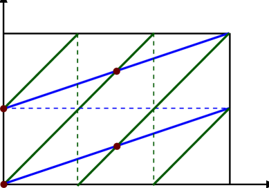
Figure 7.2: Two branes with wrapping numbers (2,1) and (3,2) intersecting four times on a $T^{2}$.

Here

$$P_{m}(L_{\|\alpha})=\eta^{-1}\,\sum_{m}q^{{\alpha^{\prime}\over 2}(m/L_{\|\alpha})^{2}}\quad{\rm and}\qquad W_{n}(L_{\perp\alpha})=\eta^{-1}\sum_{n}q^{{1\over 2\alpha^{\prime}}(nL_{\perp\alpha})^{2}}$$

denote the momentum and winding lattice sums, while we have endowed the $SO(8)$ characters with additional labels, reflecting the mass-shift of the string oscillators induced by the non-trivial intersection angle. In particular, for this $T^{2}$ reduction

$$(V_{8}-S_{8})[{\textstyle{\alpha\beta\atop\gamma\delta}}]=V_{6}\,O_{2}(\zeta)+O_{6}\,V_{2}(\zeta)-S_{6}\,S_{2}(\zeta)-C_{6}\,C_{2}(\zeta)\,,$$

with

$$\zeta={1\over\pi}\left[(\phi_{\alpha}-\phi_{\beta}){i\tau_{2}\over 2}+\phi_{\gamma}-\phi_{\delta}\right]\,,$$

$\tau_{2}$ being the proper time of the annulus and of the Möbius-strip, and we use a barred index to define the angle $\phi_{\bar{\alpha}}=-\phi_{\alpha}$ of the image brane, whose wrapping numbers are $(q_{\bar{\alpha}},k_{\bar{\alpha}})=(q_{\alpha},-k_{\alpha})$. The $SO(2)$ characters are defined by

$$O_{2}(\zeta) = {e^{2i\pi\zeta}\over 2\eta}\,\left[\theta_{3}(\zeta|\tau)+\theta_{4}(\zeta|\tau)\right],\qquad V_{2}(\zeta)={e^{2i\pi\zeta}\over 2\eta}\,\left[\theta_{3}(\zeta|\tau)-\theta_{4}(\zeta|\tau)\right]\,,$$

$$\qquad S_{2}(\zeta) = {e^{2i\pi\zeta}\over 2\eta}\,\left[\theta_{2}(\zeta|\tau)+i\theta_{1}(\zeta|\tau)\right]\,,\qquad C_{2}(\zeta)={e^{2i\pi\zeta}\over 2\eta}\,\left[\theta_{2}(\zeta|\tau)-i\theta_{1}(\zeta|\tau)\right]\,,$$

with the argument of the theta functions now depending on the relative angle, and $\tau$ the Teichmüller parameter of the double covering torus, i.e. $\tau=i\tau_{2}/2$ for the annulus amplitude and $\tau=(1+i\tau_{2})/2$ for the Möbius-strip amplitude. Finally,

$$\Upsilon_{1}[{\textstyle{\alpha\beta\atop\gamma\delta}}]={e^{2i\pi\zeta}\,\theta_{1}(\zeta|\tau)\over i\eta}\,,$$

encodes the contribution of the rotated world-sheet bosonic coordinates. Notice the multiplicative factor $2q_{\alpha}k_{\alpha}$ in the unoriented sector. It has a simple geometrical interpretation in terms of the number of times a brane and its image intersect on the $T^{2}$. More generally, two branes with wrapping numbers $(q_{\alpha},k_{\alpha})$ and $(q_{\beta},k_{\beta})$ intersect a number of times given by (see fig. 2)

$$I_{\alpha\beta}=q_{\beta}k_{\alpha}-q_{\alpha}k_{\beta}\,,$$

its sign determining the chirality of massless fermions living at the intersection points [120, 121, 122, 123, 124].

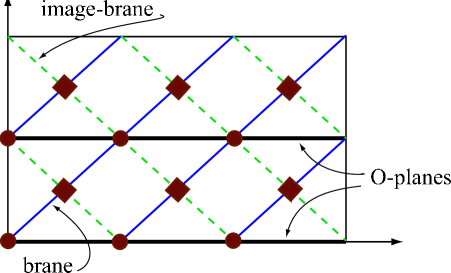
Figure 7.3: A brane (solid line) and its image (dashed line). The intersections denoted with a dot lie on the orientifold planes while those denoted with a diamond do not, and thus do not contribute to the Möbius amplitude.

To conclude this brief review on intersecting branes, the Möbius-strip amplitude

$$\mathcal{M}=-{\textstyle{1\over 2}}\left(N_{\alpha}\,(\hat{V}_{8}-\hat{S}_{8})[{\textstyle{\alpha\bar{\alpha}\atop 0}}]+\bar{N}_{\alpha}\,(\hat{V}_{8}-\hat{S}_{8})[{\textstyle{\bar{\alpha}\alpha\atop 0}}]\right)\,{K_{\alpha}\over\hat{\Upsilon}_{1}[{\textstyle{\alpha\bar{\alpha}\atop 0}}]}$$

receives contributions only from those $K_{\alpha}=2k_{\alpha}$ intersections that live on the orientifold planes (see fig. 7.3). As a result, the massless spectrum will in general contain both symmetric and antisymmetric representations of the unitary $U(N_{\alpha})$ gauge group

7.2.2 Wilson lines and brane displacements

As in the more conventional case of space-filling or point-like branes, one has the option of deforming the previous spectrum by introducing suitable Wilson lines [75] or by displacing the branes in the space transverse to their world volume [69]. This simply amounts to the deformed zero-mode mass spectrum

$$M^{2}_{\rm z.m.}(a,c)=\left({m\over L_{\|}}+a\right)^{2}+{1\over\alpha^{\prime}{}^{2}}(wL_{\perp}+c)^{2}\,.$$

It is then clear that for arbitrary values of $a$ and $c$ the open-string excitations are massive, while massless states emerge if

$$a={\mu\over L_{\|}}\,,\qquad c=\nu L_{\perp}\,,$$

for $\mu$ and $\nu$ integers. The latter condition simply reflects a symmetry under a rigid translation of the brane by an integer multiple of the distance between two consecutive wrappings.

The corresponding modifications of the annulus partition function are then quite natural. Considering for simplicity the case of an orthogonal displacement $c=\delta L_{\perp}$ of $M_{\alpha}$ branes, that still have the same wrapping numbers, one has

$$\mathcal{A} = (V_{8}-S_{8})[{\textstyle{0\atop 0}}]\,P_{m}(L_{\|})[(N_{\alpha}\bar{N}_{\alpha}+M_{\alpha}\bar{M}_{\alpha})W_{n}(L_{\perp})$$ (7.4)

$$+ N_{\alpha}\bar{M}_{\alpha}W_{n-\delta}(L_{\perp})+\bar{N}_{\alpha}M_{\alpha}W_{n+\delta}(L_{\perp})]$$

$$+ {\textstyle{1\over 2}}\bigg{[}\left(N_{\alpha}^{2}+M_{\alpha}^{2}+2N_{\alpha}M_{\alpha}\right)(V_{8}-S_{8})[{\textstyle{\alpha\bar{\alpha}\atop 0}}]$$

$$+ \left(\bar{N}_{\alpha}^{2}+\bar{M}_{\alpha}^{2}+2\bar{N}_{\alpha}\bar{M}_{\alpha}\right)(V_{8}-S_{8})[{\textstyle{\bar{\alpha}\alpha\atop 0}}]\bigg{]}\,{2q_{\alpha}k_{\alpha}\over\Upsilon_{1}[{\textstyle{\alpha\bar{\alpha}\atop 0}}]}$$

with an obvious deformation of the Möbius-strip amplitude. It is then clear that for arbitrary $\delta$ the original gauge group $U(N_{\alpha}+M_{\alpha})$ is broken to $U(N_{\alpha})\times U(M_{\alpha})$ while the (anti-)symmetric representations decompose into the sum of (anti-)symmetric representations of each group factor plus additional bi-fundamentals. As expected, for $\delta$ integer new massless vectors emerge from strings stretched between overlapping wrappings of the $N_{\alpha}$ and $M_{\alpha}$ branes and the gauge symmetmery is consequently enhanced to the original $U(N_{\alpha}+M_{\alpha})$.

7.2.3 Branes vs antibranes: an intriguing $\pi\!$uzzle

The formalism of intersecting branes here reviewed may hide some ambiguities. It is well known in fact that anti-branes (with positive tension and negative R-R charge) are nothing but regular branes (with positive tension and positive R-R charge) that have undergone a $\pi$ rotation, as shown in fig. 7.4. On a compact space, if a brane has wrapping numbers $(q,k)$ and angle $\phi$ its conjugate partner has opposite wrapping numbers $(-q,-k)$ and an angle $\phi+\pi$. Despite branes and anti-branes satisfy the same quantisation condition 7.2 and induce similar mass shifts in the spectrum of string excitations, their relative $\pi$ angle plays a crucial role in selecting the correct GSO projection.

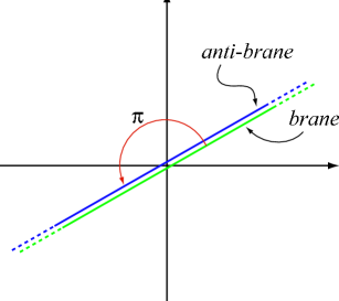
Figure 7.4: A brane and its anti-brane differing by a $\pi$ rotation.

Let us consider in fact the spectrum of open strings stretched between two branes with angles $\phi_{\alpha}$ and $\phi_{\beta}$. As already observed, it is encoded in the partition function

$${(V_{8}-S_{8})[{\textstyle{\alpha\beta\atop 0}}]\over\Upsilon_{1}[{\textstyle{\alpha\beta\atop 0}}]}\sim{V_{6}O_{2}(\zeta)+O_{6}V_{2}(\zeta)-S_{6}S_{2}(\zeta)-C_{6}C_{2}(\zeta)\over\theta_{1}(\zeta|\tau)\,q^{{1\over\pi}(\phi_{\alpha}-\phi_{\beta})}}\,,$$

with $\zeta=(\phi_{\alpha}-\phi_{\beta})\tau/\pi$, where we have omitted irrelevant numerical factors. After rotating the $\alpha$ brane, say, by an angle $\pi$ and converting it to an anti-brane, the partition function obviously reads

$${(V_{8}-S_{8})[{\textstyle{\alpha^{\prime}\beta\atop 0}}]\over\Upsilon_{1}[{\textstyle{\alpha^{\prime}\beta\atop 0}}]}\sim{V_{6}O_{2}(\zeta_{\pi})+O_{6}V_{2}(\zeta_{\pi})-S_{6}S_{2}(\zeta_{\pi})-C_{6}C_{2}(\zeta_{\pi})\over\theta_{1}(\zeta_{\pi}|\tau)\,q^{{1\over\pi}(\phi_{\alpha}-\phi_{\beta})+1}}\,,$$ (7.5)

with now $\zeta_{\pi}=(\phi_{\alpha}-\phi_{\beta}+\pi)\tau/\pi$. From the very definition of theta functions

$$\theta[{\textstyle{a\atop b}}](z|\tau)=\sum_{n}q^{{1\over 2}(n+a)^{2}}\,e^{2i\pi(n+a)(z+b)}\,,$$

one can then deduce the periodicity properties

$$\theta_{3}(\zeta_{\pi}|\tau) = +q^{-{\phi\over\pi}-{1\over 2}}\,\theta_{3}(\zeta|\tau),\qquad\theta_{2}(\zeta_{\pi}|\tau)=+q^{-{\phi\over\pi}-{1\over 2}}\,\theta_{2}(\zeta|\tau)$$

$$\theta_{4}(\zeta_{\pi}|\tau) = -q^{-{\phi\over\pi}-{1\over 2}}\,\theta_{4}(\zeta|\tau)\,,\qquad\theta_{1}(\zeta_{\pi}|\tau)=-q^{-{\phi\over\pi}-{1\over 2}}\,\theta_{1}(\zeta|\tau)\,,$$ (7.6)

that, in turn, induce a non-trivial reshuffling of the SO(2) characters

$$\eqalign{O_{2}(\zeta_{\pi})=&V_{2}(\zeta)\,q^{-{\phi\over\pi}+{1\over 2}}\,,\cr V_{2}(\zeta_{\pi})=&O_{2}(\zeta)\,q^{-{\phi\over\pi}+{1\over 2}}\,,\cr}\qquad\eqalign{S_{2}(\zeta_{\pi})=&C_{2}(\zeta)\,q^{-{\phi\over\pi}+{1\over 2}}\,,\cr C_{2}(\zeta_{\pi})=&S_{2}(\zeta)\,q^{-{\phi\over\pi}+{1\over 2}}\,.\cr}$$

As a result, the GSO projection in (7.5) changes to

$${(V_{8}-S_{8})[{\textstyle{\alpha^{\prime}\beta\atop 0}}]\over\Upsilon_{1}[{\textstyle{\alpha^{\prime}\beta\atop 0}}]}\sim{V_{6}V_{2}(\zeta)+O_{6}O_{2}(\zeta)-S_{6}C_{2}(\zeta)-C_{6}S_{2}(\zeta)\over\theta_{1}(\zeta|\tau)\,q^{{1\over\pi}(\phi_{\alpha}-\phi_{\beta})}}\,,$$

that indeed pertains to open strings stretched between pairs of branes and anti-branes [116].

It is evident, that the formalism introduced in sub-sections 7.2.1 and 7.2.2 is well tailored to study any kind of brane if care is used in dealing with apparently innocuous $\pi$ angles. To avoid ambiguities, in this paper we adopt the convention to use the term brane when $q$ is positive, and anti-brane when $q$ is negative. This is clearly suggested by their contribution to the R-R tadpoles. Then according to the sign of their vertical wrapping number $k$, they can induce positive or negative charges for lower-degree gauge potentials, and consequently transmute into lower-dimensional branes (for $k>0$) or anti-branes (for $k<0$).

7.3 Freely acting orbifolds, Scherk-Schwarz deformations and intersecting branes

We can now turn to the study of the effects freely acting shifts have on rotated and intersecting branes. For simplicity we shall focus to the case of a $\mathbb{Z}_{2}$ shift, although similar considerations can be straightforwardly extended to the more general case. On a given $T^{2}$ one has in principle to distinguish among the three cases of shifts acting along the horizontal axis only, along the vertical axis only or along both the horizontal and vertical axis. It turns out that it is enough to consider one case, since the others can be unambiguously determined. To this end, let us consider the shift

$$\delta:\quad\left\{\eqalign{y_{1}&\to y_{1}+{\textstyle{1\over 2}}R_{1}\,,\cr y_{2}&\to y_{2}\,,\cr}\right.$$

where $(y_{1},y_{2})$ are the natural coordinates on a rectangular torus with sides of length $R_{1}$ and $R_{2}$. With respect to the natural reference frame adapted to the brane this $\mathbb{Z}_{2}$ shift decomposes as

$$\delta:\quad\left\{\eqalign{\bar{y}_{1}&\to\bar{y}_{1}+{\textstyle{1\over 2}}R_{1}\cos\phi\,,\cr\bar{y}_{2}&\to\bar{y}_{2}-{\textstyle{1\over 2}}R_{1}\sin\phi\,,\cr}\right.$$

with $\bar{y}_{1}$ and $\bar{y}_{2}$ labelling the directions longitudinal and transverse to the brane, respectively. This shift maps in general points on the branes to points in the bulk unless ($\mu\in\mathbb{Z}$)

$$y_{2}+\mu R_{2}=\tan\phi\left(y_{1}+{\textstyle{1\over 2}}R_{1}\right)\quad\Rightarrow\quad\mu R_{2}={kR_{2}\over 2q}\quad\Rightarrow\quad k\in 2\mathbb{Z}\,,$$

that is to say that the shifted point still belongs to the line identified by the brane, modulo ${\rm SL}(2,\mathbb{Z})$ identifications of the lattice.

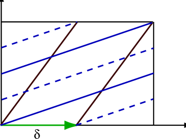
Figure 7.5: The two classes of branes in the presence of a freely acting horizontal shift $\delta$. The dashed brane is the image under $\delta$.

It is then evident that we can identify two equivalence classes of branes, as indicated in figure 7.5: those with odd $k$ and those with even $k$. In the former case the shift is not a symmetry unless we introduce image branes with the same angle but separated by a distance $-{\textstyle{1\over 2}}R_{1}\sin\phi$. In the latter case the shifted points still belong to the brane and thus the given configuration is already symmetric under the action of $\delta$. Similarly, for shifts along the vertical axis (or along the diagonal of the torus) only for branes with $q$ even (or with $k$ and $q$ both odd) the image points still belong to the brane world volume. This is somewhat reminiscent of what happens when we act with freely acting shifts along the world-volume of the brane and or along directions transverse to it.

Given these observations, it is straightforward to write down the associated vacuum amplitudes. Since in this toy model we are modding out by $\Omega\mathscr{R}$, our parent theory is the type IIA superstring compactified on a $T^{2}$

$$\mathcal{T}=(V_{8}-S_{8})(\bar{V}_{8}-\bar{C}_{8})\,\left[\Lambda_{2m_{1},n_{1}}(R_{1})\Lambda_{m_{2},n_{2}}(R_{2})+\Lambda_{2m_{1},n_{1}+{1\over 2}}(R_{1})\Lambda_{m_{2},n_{2}}(R_{2})\right]\,,$$

where each $\Lambda(R)$ denotes the Narain lattice for a circle of radius $R$ and momenta and windings specified. The associated direct-channel Klein-bottle amplitude reads

$$\mathcal{K}={\textstyle{1\over 2}}(V_{8}-S_{8})\,P_{2m_{1}}(R_{1})W_{n_{2}}(R_{2})\,.$$

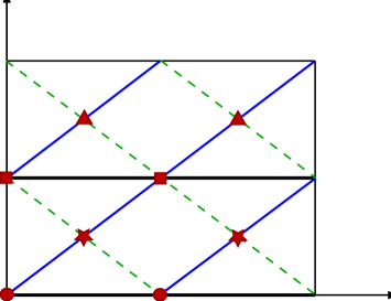
Figure 7.6: A (1,1) brane and its images under $\Omega\mathscr{R}$ and $\delta$. The intersections marked with alike symbols are identified under $\delta$.

Moving to the open-string sector, for $k_{\alpha}$ odd, the direct-channel annulus and Möbius-strip amplitudes now read

$$\eqalign{\mathcal{A}=&N_{\alpha}\bar{N}_{\alpha}\,(V_{8}-S_{8})[{\textstyle{0\atop 0}}]P_{m}\left[W_{n}+W_{n+{1\over 2}}\right]\cr&+{\textstyle{1\over 2}}\,\left[N^{2}_{\alpha}\,(V_{8}-S_{8})[{\textstyle{\alpha\bar{\alpha}\atop 0}}]+\bar{N}^{2}_{\alpha}\,(V_{8}-S_{8})[{\textstyle{\bar{\alpha}\alpha\atop 0}}]\right]\,{2I_{\alpha\bar{\alpha}}\over\Upsilon_{1}[{\textstyle{\alpha\bar{\alpha}\atop 0}}]}\,,\cr}$$

and

$$\mathcal{M}=-{\textstyle{1\over 2}}\left[N_{\alpha}\,(\hat{V}_{8}-\hat{S}_{8})[{\textstyle{\alpha\bar{\alpha}\atop 0}}]+\bar{N}_{\alpha}\,(\hat{V}_{8}-\hat{S}_{8})[{\textstyle{\bar{\alpha}\alpha\atop 0}}]\right]{K_{\alpha}\over\hat{\Upsilon}_{1}[{\textstyle{\alpha\bar{\alpha}\atop 0}}]}\,.$$

Notice the important difference with the standard case: the annulus amplitude unambiguously reflects the presence of image branes under the action of the horizontal shift both by the presence of dipole strings with shifted windings, and by the doubling of the number of families for unoriented strings due to the doubling of local intersections. As for the Möbius-strip amplitude, instead, it is not modified since the effective number of intersections sitting on the O-planes is not affected. This counting of effective intersections is clearly depicted in figure 7.6 in the case of (1,1) branes, where points marked with the same symbol are identified under $\delta$.

Moving to the case of branes with even $k_{\alpha}$, one is not required any longer to introduce brane images, these branes being invariant under $\delta$, and the annulus and Möbius-strip amplitudes read

$$\eqalign{\mathcal{A}=&N_{\alpha}\bar{N}_{\alpha}\,(V_{8}-S_{8})[{\textstyle{0\atop 0}}]P_{2m}W_{n}\cr+&{\textstyle{1\over 2}}\left[N^{2}_{\alpha}\,(V_{8}-S_{8})[{\textstyle{\alpha\bar{\alpha}\atop 0}}]+\bar{N}^{2}_{\alpha}\,(V_{8}-S_{8})[{\textstyle{\bar{\alpha}\alpha\atop 0}}]\right]\,{I_{\alpha\bar{\alpha}}\over 2\Upsilon_{1}[{\textstyle{\alpha\bar{\alpha}\atop 0}}]}\,,\cr}$$

and

$$\mathcal{M}=-{\textstyle{1\over 2}}\left[N_{\alpha}\,(\hat{V}_{8}-\hat{S}_{8})[{\textstyle{\alpha\bar{\alpha}\atop 0}}]+\bar{N}_{\alpha}\,(\hat{V}_{8}-\hat{S}_{8})[{\textstyle{\bar{\alpha}\alpha\atop 0}}]\right]{K_{\alpha}\over 2\hat{\Upsilon}_{1}[{\textstyle{\alpha\bar{\alpha}\atop 0}}]}\,.$$

In contrast to the previous case, the multiplicities in the annulus and Möbius-strip amplitudes have now been halved, since $\delta$ identifies pairs of intersection points, as depicted in figure 7.7.

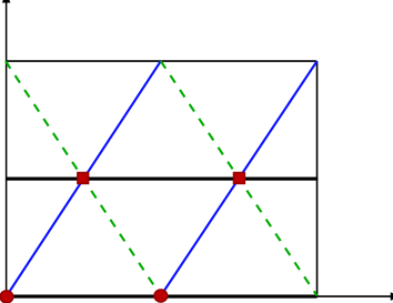
Figure 7.7: A (1,1) brane and its images under $\Omega\mathscr{R}$ and $\delta$. The intersections marked with alike symbols are identified under $\delta$.

We can now straightforwardly generalise the open-string amplitudes to the case of a more interesting $T^{6}=T^{2}\times T^{2}\times T^{2}$ compactification with the shift acting along the horizontal axis $y_{1}$ of the first $T^{2}$. For simplicity we shall focus our attention to the case of factorisable D6 branes or, in the T-dual language, to commuting magnetic backgrounds, although more general choices turned out to be very promising in stabilising closed-string moduli [127],[128]. In this simple case, D6 branes on a $T^{2}\times T^{2}\times T^{2}$ are then identified by their angles $\phi^{\Lambda}_{\alpha}$ ($\Lambda=1,2,3$ labelling the three two-tori) and wrapping numbers $(q_{\alpha}^{\Lambda}\,,\,k^{\Lambda}_{\alpha})$ related, as usual, by

$$\tan\phi^{\Lambda}_{\alpha}={k^{\Lambda}_{\alpha}\,R^{\Lambda}_{2}\over q^{\Lambda}_{\alpha}\,R^{\Lambda}_{1}}\,,$$

where $R^{\Lambda}_{1}$ and $R^{\Lambda}_{2}$ denote the sizes of the horizontal and vertical sides of the $\Lambda$-th $T^{2}$, respectively. We then split the generic index $\alpha$ into the pair $a$ and $i$ labelling respectively $n_{\rm o}$ different stacks of $N_{a}$ branes ($a=1,\ldots,n_{\rm o}$) with $k^{1}_{a}$ odd and $n_{\rm e}$ different stacks of $N_{i}$ branes ($i=1,\ldots,n_{\rm e}$) with $k^{1}_{i}$ even. The annulus amplitude is then

$$\mathcal{A} = \sum_{a=1}^{n_{\rm o}}N_{a}\bar{N}_{a}\,(V_{8}-S_{8})[{\textstyle{0\atop 0}}]\,P_{m}^{1}\left[W_{n}^{1}+W_{n+{1\over 2}}^{1}\right]P_{m}^{2}W_{n}^{2}P_{m}^{3}W_{n}^{3}$$ (7.7)

$$+ \sum_{i=1}^{n_{\rm e}}N_{i}\bar{N}_{i}\,(V_{8}-S_{8})[{\textstyle{0\atop 0}}]\,P_{2m}^{1}W_{n}^{1}P_{m}^{2}W_{n}^{2}P_{m}^{3}W_{n}^{3}$$

$$+ {\textstyle{1\over 2}}\sum_{a=1}^{n_{\rm o}}\left(N_{a}^{2}(V_{8}-S_{8})[{\textstyle{a\bar{a}\atop 0}}]+\bar{N}_{a}^{2}(V_{8}-S_{8})[{\textstyle{\bar{a}a\atop 0}}]\right)\,{2I_{a\bar{a}}\over\Upsilon_{1}[{\textstyle{a\bar{a}\atop 0}}]}$$

$$+ {\textstyle{1\over 2}}\sum_{i=1}^{n_{\rm e}}\left(N_{i}^{2}(V_{8}-S_{8})[{\textstyle{i\bar{\imath}\atop 0}}]+\bar{N}_{i}^{2}(V_{8}-S_{8})[{\textstyle{\bar{\imath}i\atop 0}}]\right)\,{I_{i\bar{\imath}}\over 2\,\Upsilon_{1}[{\textstyle{i\bar{\imath}\atop 0}}]}$$

$$+ \sum_{{a,b=1\atop b<a}}^{n_{\rm o}}\left(N_{a}\bar{N}_{b}(V_{8}-S_{8})[{\textstyle{ab\atop 0}}]+\bar{N}_{a}N_{b}(V_{8}-S_{8})[{\textstyle{\bar{a}\bar{b}\atop 0}}]\right)\,{2\,I_{ab}\over\Upsilon_{1}[{\textstyle{ab\atop 0}}]}$$

$$+ \sum_{{a,b=1\atop b<a}}^{n_{\rm o}}\left(N_{a}N_{b}(V_{8}-S_{8})[{\textstyle{a\bar{b}\atop 0}}]+\bar{N}_{a}\bar{N}_{b}(V_{8}-S_{8})[{\textstyle{\bar{a}b\atop 0}}]\right)\,{2\,I_{a\bar{b}}\over\Upsilon_{1}[{\textstyle{a\bar{b}\atop 0}}]}$$

$$+ \sum_{{i,j=1\atop j<i}}^{n_{\rm e}}\left(N_{i}\bar{N}_{j}(V_{8}-S_{8})[{\textstyle{ij\atop 0}}]+\bar{N}_{i}N_{j}(V_{8}-S_{8})[{\textstyle{\bar{\imath}\bar{\jmath}\atop 0}}]\right)\,{I_{ij}\over 2\,\Upsilon_{1}[{\textstyle{ij\atop 0}}]}$$

$$+ \sum_{{i,j=1\atop j<i}}^{n_{\rm e}}\left(N_{i}N_{j}(V_{8}-S_{8})[{\textstyle{i\bar{\jmath}\atop 0}}]+\bar{N}_{i}\bar{N}_{j}(V_{8}-S_{8})[{\textstyle{\bar{\imath}j\atop 0}}]\right)\,{I_{i\bar{\jmath}}\over 2\,\Upsilon_{1}[{\textstyle{i\bar{\jmath}\atop 0}}]}$$

$$+ \sum_{a=1}^{n_{\rm o}}\sum_{i=1}^{n_{\rm e}}\left(N_{a}\bar{N}_{i}\,(V_{8}-S_{8})[{\textstyle{ai\atop 0}}]+\bar{N}_{a}N_{i}\,(V_{8}-S_{8})[{\textstyle{\bar{a}\bar{\imath}\atop 0}}]\right)\,{I_{ai}\over\Upsilon_{1}[{\textstyle{ai\atop 0}}]}$$

$$+ \sum_{a=1}^{n_{\rm o}}\sum_{i=1}^{n_{\rm e}}\left(N_{a}N_{i}\,(V_{8}-S_{8})[{\textstyle{a\bar{\imath}\atop 0}}]+\bar{N}_{a}\bar{N}_{i}\,(V_{8}-S_{8})[{\textstyle{\bar{a}i\atop 0}}]\right)\,{I_{a\bar{\imath}}\over\Upsilon_{1}[{\textstyle{a\bar{\imath}\atop 0}}]}$$

To lighten the notation, we omit here and in following similar expressions the “effective radius” dependence of the various momentum and winding lattice contributions. In particular, $P_{m}^{\Lambda}$ ($W_{n}^{\Lambda}$) is a short-hand notation for $P_{m}(L_{\alpha\|}^{\Lambda})$ ($W_{n}(L_{\alpha\perp}^{\Lambda})$), where $L_{\alpha\|}^{\Lambda}$ ($L_{\alpha\perp}^{\Lambda}$) is the total length (the transverse distance among the consecutive wrappings) of the $\alpha$-th stack of branes in the $\Lambda$-th torus. The Möbius-strip amplitude instead is a simple combination of the previous ones and reads

$$\eqalign{\mathcal{M}=&-{\textstyle{1\over 2}}\sum_{a=1}^{n_{\rm o}}\left(N_{a}\,(\hat{V}_{8}-\hat{S}_{8})[{\textstyle{a\bar{a}\atop 0}}]+\bar{N}_{a}\,(\hat{V}_{8}-\hat{S}_{8})[{\textstyle{\bar{a}a\atop 0}}]\right){K_{a}\over\hat{\Upsilon}_{1}[{\textstyle{a\bar{a}\atop 0}}]}\cr&-{\textstyle{1\over 2}}\sum_{i=1}^{n_{\rm e}}\left(N_{i}\,(\hat{V}_{8}-\hat{S}_{8})[{\textstyle{i\bar{\imath}\atop 0}}]+\bar{N}_{i}\,(\hat{V}_{8}-\hat{S}_{8})[{\textstyle{\bar{\imath}i\atop 0}}]\right){K_{i}\over 2\,\hat{\Upsilon}_{1}[{\textstyle{i\bar{\imath}\atop 0}}]}\,.\cr}$$

Here we have adapted our notation to the case of multiple $T^{2}$’s. As already stated we append an index $\Lambda$ to angles and wrapping numbers relative to the $\Lambda$-th torus, while now

$$I_{\alpha\beta}=\prod_{\Lambda=1}^{3}\,\left(q_{\beta}^{\Lambda}\,k_{\alpha}^{\Lambda}-q_{\alpha}^{\Lambda}\,k_{\beta}^{\Lambda}\right)$$

and

$$K_{\alpha}=\prod_{\Lambda=1,2,3}\,2\,k^{\Lambda}_{\alpha}$$

count the total number of intersections in the $T^{6}$, and those sitting on the O6 planes. Moreover, the contribution of the world-sheet bosons is

$$\Upsilon_{1}\,[{\textstyle{\alpha\beta\atop\gamma\delta}}]=\prod_{\Lambda=1,2,3}\,{\theta_{1}(\zeta^{\Lambda}|\tau)\over i\eta(\tau)}\,e^{2i\pi\zeta^{\Lambda}}\,,$$

with

$$\zeta^{\Lambda}={1\over\pi}\left[\left(\phi^{\Lambda}_{\alpha}-\phi^{\Lambda}_{\beta}\right)\tau+\left(\phi_{\gamma}^{\Lambda}-\phi_{\delta}^{\Lambda}\right)\right]\,.$$

The contribution of the world-sheet fermions is more involved and requires an $SO(8)\to SO(2)\times SO(2)\times SO(2)\times SO(2)$ breaking of the original characters. This is a consequence of the fact that, in the T-dual language of magnetised backgrounds, fields with different helicities couple differently to the magnetic fields. More explicitly

$$\eqalign{V_{8}\,[{\textstyle{\alpha\beta\atop\gamma\delta}}]=V_{2}&\,\left[O_{2}(\zeta^{1})\,O_{2}(\zeta^{2})\,O_{2}(\zeta^{3})+O_{2}(\zeta^{1})\,V_{2}(\zeta^{2})\,V_{2}(\zeta^{3})\right.\cr&\left.+V_{2}(\zeta^{1})\,V_{2}(\zeta^{2})\,O_{2}(\zeta^{3})+V_{2}(\zeta^{1})\,O_{2}(\zeta^{2})\,V_{2}(\zeta^{3})\right]\cr+O_{2}&\,\left[V_{2}(\zeta^{1})\,O_{2}(\zeta^{2})\,O_{2}(\zeta^{3})+V_{2}(\zeta^{1})\,V_{2}(\zeta^{2})\,V_{2}(\zeta^{3})\right.\cr&\left.+O_{2}(\zeta^{1})\,V_{2}(\zeta^{2})\,O_{2}(\zeta^{3})+O_{2}(\zeta^{1})\,O_{2}(\zeta^{2})\,V_{2}(\zeta^{3})\right]\,,\cr S_{8}\,[{\textstyle{\alpha\beta\atop\gamma\delta}}]=S_{2}&\,\left[S_{2}(\zeta^{1})\,S_{2}(\zeta^{2})\,S_{2}(\zeta^{3})+S_{2}(\zeta^{1})\,C_{2}(\zeta^{2})\,C_{2}(\zeta^{3})\right.\cr&\left.+C_{2}(\zeta^{1})\,S_{2}(\zeta^{2})\,C_{2}(\zeta^{3})+C_{2}(\zeta^{1})\,C_{2}(\zeta^{2})\,S_{2}(\zeta^{3})\right]\cr+C_{2}&\,\left[C_{2}(\zeta^{1})\,S_{2}(\zeta^{2})\,S_{2}(\zeta^{3})+C_{2}(\zeta^{1})\,C_{2}(\zeta^{2})\,C_{2}(\zeta^{3})\right.\cr&\left.+S_{2}(\zeta^{1})\,S_{2}(\zeta^{2})\,C_{2}(\zeta^{3})+S_{2}(\zeta^{1})\,C_{2}(\zeta^{2})S_{2}(\zeta^{3})\right]\,.\cr}$$

As usual, the massless spectrum can be extracted expanding $\mathcal{A}$ and $\mathcal{M}$. Aside from the full $\mathscr{N}=4$ super-Yang-Mills multiplet in the adjoint representation of the Chan-Paton gauge group, one typically gets tachyonic excitations and (non-)chiral fermions in various representations. The spectrum of chiral fermions can be easily computed and is encoded in table 1, where, as usual, $A_{\alpha}$ and $S_{\alpha}$ denote respectively the anti-symmetric and symmetric representations of the $\alpha$-th factor in the gauge group. As for non-chiral fermions, these emerge whenever branes are parallel in a given $T^{2}$. Their multiplicity is then given by the number of times the corresponding branes intersect in the remaining tori. For instance, if the branes of type $\alpha$ and $\beta$ are parallel in the first $T^{2}$, then one finds

$$I^{\rm non\ chiral}_{\alpha\beta}=\prod_{\Sigma=2,3}\left(q_{\beta}^{\Sigma}\,k^{\Sigma}_{\alpha}-q_{\alpha}^{\Sigma}\,k^{\Sigma}_{\beta}\right)$$

non-chiral fermions in the representation $(N_{\alpha},\bar{N}_{\beta})$.

Rep.	multiplicity
$A_{a}$	$\quad\quad{1\over 2}(2\,I_{a\bar{a}}\pm K_{a})$
$S_{a}$	$\quad\quad{1\over 2}(2\,I_{a\bar{a}}\mp K_{a})$
$A_{i}$	$\quad\quad{1\over 4}(I_{i\bar{\imath}}\pm K_{i})$
$S_{i}$	$\quad\quad{1\over 4}(I_{i\bar{\imath}}\mp K_{i})$
$(N_{a},N_{b})$	$\quad\quad 2\,I_{a\bar{b}}$
$(N_{a},\bar{N}_{b})$	$\quad\quad 2\,I_{ab}$
$(N_{i},N_{j})$	$\quad\quad{1\over 2}\,I_{i\bar{\jmath}}$
$(N_{i},\bar{N}_{j})$	$\quad\quad{1\over 2}\,I_{ij}$
$(N_{a},N_{i})$	$\quad\quad I_{a\bar{\imath}}$
$(N_{a},\bar{N}_{i})$	$\quad\quad I_{ai}$

Table 7.1: Spectrum of four-dimensional chiral fermions. The sign of $I_{\alpha\bar{\beta}}$ determines the chirality of the four-dimensional spinors, while the two signs in the multiplicity of (anti-)symmetric representations refer to branes ($q>0$) or to anti-branes ($q<0$), respectively.

Turning to the transverse channel, the massless tadpoles can be extracted as usual from the leading terms in $\tilde{\mathcal{K}}$, $\tilde{\mathcal{A}}$ and $\tilde{\mathcal{M}}$. Introducing the combinations

$${\bf R}=\prod_{\Lambda=1}^{3}\,\sqrt{R_{1}^{\Lambda}\over R_{2}^{\Lambda}}\,,\qquad{\bf L}_{\alpha}=\prod_{\Lambda=1}^{3}\,\sqrt{L^{\Lambda}_{\|\,\alpha}\over L^{\Lambda}_{\perp\,\alpha}}\,,$$ (7.8)

the NS-NS dilaton tadpole reads

$$2\,\sum_{a=1}^{n_{\rm o}}\,{\bf L}_{a}\,\left(N_{a}+\bar{N}_{a}\right)+\sum_{i=1}^{n_{\rm e}}\,{\bf L}_{i}\,\left(N_{i}+\bar{N}_{i}\right)=2^{5}\,{\bf R}\,.$$ (7.9)

Notice that, after a T-duality along the vertical axis, the left-hand-side is nothing but the Dirac-Born-Infeld Action

$${\bf L_{\alpha}}=\prod_{\Lambda=1,2,3}\,\sqrt{R_{1}R_{2}\,{\rm det}\,\left[q^{\Lambda}_{\alpha}\,\left({\bf 1}+F^{\Lambda}_{\alpha}\right)\right]}\,,$$

with $F^{\Lambda}$ a two-by-two antisymmetric matrix, whose only independent entry is the magnetic field background $H^{\Lambda}$. The eight different R-R tadpoles can be straightforwardly obtained from (7.9) after a multiplication of the Chan-Paton multiplicities by a phase depending on the scalar product of the rotation angles $\phi^{\Lambda}_{\alpha}$ and the helicities $\eta^{\Lambda}=\pm{1\over 2}$ of the internal spinors. With our convention such that $S_{2}$ has helicity $+{1\over 2}$ and $C_{2}$ has helicity $-{1\over 2}$, they read

$$2\,\sum_{a=1}^{n_{\rm o}}\,{\bf L}_{a}\,\left(N_{a}\,e^{2i\phi_{a}\cdot\eta}+\bar{N}_{a}\,e^{-2i\phi_{a}\cdot\eta}\right)+\sum_{i=1}^{n_{\rm e}}\,{\bf L}_{i}\,\left(N_{i}\,e^{2i\phi_{i}\cdot\eta}+\bar{N}_{i}\,e^{-2i\phi_{i}\cdot\eta}\right)=2^{5}\,{\bf R}\,,$$ (7.10)

with the internal product $\phi_{\alpha}\cdot\eta=\sum_{\Lambda=1}^{3}\,\phi_{\alpha}^{\Lambda}\,\eta^{\Lambda}$. This single R-R tadpole actually encodes couplings to different forms as dictated by the (T-dualised) Action

$$S\sim\int\,\sum_{p}\,C_{p+1}\,e^{iF}\sim\int\,C_{10}+i\,C_{8}\wedge F-{\textstyle{1\over 2}}\,C_{6}\wedge F\wedge F-{\textstyle{1\over 6}}\,i\,C_{4}\wedge F\wedge F\wedge F\,.$$

Each factor, in turn, receives contributions from several terms according to which internal $T^{2}$ the magnetic field points to. For instance, the real part of the tadpole (7.10) yields the conditions

$$\eqalign{\left[\sum_{a=1}^{n_{o}}\,2\,q^{1}_{a}\,q^{2}_{a}\,q^{3}_{a}\,N_{a}+\sum_{i=1}^{n_{e}}\,q^{1}_{i}\,q^{2}_{i}\,q^{3}_{i}\,N_{i}\right]\sqrt{R^{1}_{1}\,R^{2}_{1}\,R^{3}_{1}\over R_{2}^{1}\,R_{2}^{2}\,R_{2}^{3}}=&16\,\sqrt{R^{1}_{1}\,R^{2}_{1}\,R^{3}_{1}\over R_{2}^{1}\,R_{2}^{2}\,R_{2}^{3}}\,,\cr\left[\sum_{a=1}^{n_{o}}\,2\,q^{1}_{a}\,k^{2}_{a}\,k^{3}_{a}\,N_{a}+\sum_{i=1}^{n_{e}}\,q^{1}_{i}\,k^{2}_{i}\,k^{3}_{i}\,N_{i}\right]\sqrt{R^{1}_{1}\,R^{2}_{2}\,R^{3}_{2}\over R_{2}^{1}\,R_{1}^{2}\,R_{1}^{3}}=&0\,,\cr\left[\sum_{a=1}^{n_{o}}\,2\,k^{1}_{a}\,q^{2}_{a}\,k^{3}_{a}\,N_{a}+\sum_{i=1}^{n_{e}}\,k^{1}_{i}\,q^{2}_{i}\,k^{3}_{i}\,N_{i}\right]\sqrt{R^{1}_{2}\,R^{2}_{1}\,R^{3}_{2}\over R_{1}^{1}\,R_{2}^{2}\,R_{1}^{3}}=&0\,,\cr\left[\sum_{a=1}^{n_{o}}\,2\,k^{1}_{a}\,k^{2}_{a}\,q^{3}_{a}\,N_{a}+\sum_{i=1}^{n_{e}}\,k^{1}_{i}\,k^{2}_{i}\,q^{3}_{i}\,N_{i}\right]\sqrt{R^{1}_{2}\,R^{2}_{2}\,R^{3}_{1}\over R_{1}^{1}\,R_{1}^{2}\,R_{2}^{3}}=&0\,.\cr}$$

After the vertical axis of the three $T^{2}$’s are properly T dualised, one can then read the couplings with the ten-form potential $C_{10}$ and with the three six-form potentials $C^{\Lambda}_{6}$, whose six indices point to the four non-compact space-time directions and to the two compact coordinates of the $\Lambda$-th torus. The imaginary part of the tadpole (7.10) is proportional to $N_{\alpha}-\bar{N}_{\alpha}$ and thus vanishes identically. This is fully consistent with the fact that the $C_{8}$ and $C_{4}$ forms are projected out by the orientifold involution and thus do not belong to the physical spectrum.

7.3.1 Breaking supersymmetry in the dipole-string sector

After we have learned how shifts act on rotated branes, we can now proceed to the study of the combined effect of $\delta$ and $(-1)^{F}$. As is well known the (freely-acting) orbifold generated by $\delta\,(-1)^{F}$ is a convenient string description of Sherck-Schwarz deformations that in general are responsible for giving masses to fermions, and thus for breaking supersymmetry. Following the lines of section 7.3 we expect that the space-time fermion index has a non trivial effect only when the shift $\delta$ moves points along the brane, that is only when $k_{i}$ is an even number. In this case the annulus amplitude reads

$$\mathcal{A} = N_{i}\bar{N}_{i}\,\big{(}V_{8}[{\textstyle{0\atop 0}}]\,P_{2m}-S_{8}[{\textstyle{0\atop 0}}]\,P_{2m+1}\big{)}\,W_{n}$$ (7.11)

$$+ {\textstyle{1\over 2}}\left(N^{2}_{i}\,(V_{8}-S_{8})[{\textstyle{i\bar{\imath}\atop 0}}]+\bar{N}^{2}_{i}(V_{8}-S_{8})[{\textstyle{\bar{\imath}i\atop 0}}]\right)\,{I_{i\bar{\imath}}\over 2\,\Upsilon_{1}[{\textstyle{i\bar{\imath}\atop 0}}]}$$

As is spelled out by this direct-channel amplitude, the adjoint fermions have now got a mass

$$m_{1/2}\sim L_{\|}^{-1}={\cos\phi_{i}\over q_{i}R_{1}}={\sqrt{1+\alpha^{\prime}{}^{2}H_{i}^{2}}\over q_{i}R_{1}}={1\over q_{i}^{2}\,R_{1}^{2}}\sqrt{q_{i}^{2}\,R_{1}^{2}+\alpha^{\prime}{}^{2}{k_{i}^{2}\over R_{2}^{2}}}\,,$$

of the order of the TeV, and, consequently, supersymmetry is broken in the neutral dipole-string sector. In the transverse channel

$$\eqalign{\tilde{\mathcal{A}}=&\,2^{-6}\,{L_{\|i}\over L_{\perp i}}\,N_{i}\bar{N}_{i}\,\left[(V_{8}-S_{8})[{\textstyle{0\atop 0}}]\,\tilde{W}_{n}+(O_{8}-C_{8})[{\textstyle{0\atop 0}}]\,\tilde{W}_{n+{1\over 2}}\right]\,\tilde{P}_{m}\cr&+2^{-5}\,\left[N^{2}_{i}\,(V_{8}-S_{8})[{\textstyle{0\atop i\bar{\imath}}}]+\bar{N}^{2}_{i}\,(V_{8}-S_{8})[{\textstyle{0\atop\bar{\imath}i}}]\right]\,{I_{i\bar{\imath}}\over 2\,\Upsilon_{1}[{\textstyle{0\atop i\bar{\imath}}}]}\,,\cr}$$

the twisted closed-string R-R states are massive, and the only massless tadpoles one is to worry about are those for the untwisted R-R fields in $S_{8}$.

The generalisation to higher-dimensional tori is also straightforward. The only modification is in the dipole sector of the $N_{i}$ branes that now would read

$$\sum_{i=1}^{n_{\rm e}}M_{i}\bar{M}_{i}\,\left(V_{8}\,[{\textstyle{0\atop 0}}]\,P_{2m}^{1}\,-S_{8}\,[{\textstyle{0\atop 0}}]\,P_{2m+1}^{1}\right)W_{n}^{1}P_{m}^{2}W_{n}^{2}P_{m}^{3}W_{n}^{3}\,.$$ (7.12)

It reflects itself in the transverse-channel contribution

$$2^{-6}\,\sum_{i=1}^{n_{\rm e}}\,({\bf L}^{\Lambda}_{i})^{2}\,N_{i}\bar{N}_{i}\,\Bigl{[}(V_{8}-S_{8})[{\textstyle{0\atop 0}}]\,\tilde{W}_{n}^{1}+(O_{8}-C_{8})[{\textstyle{0\atop 0}}]\,\tilde{W}_{n+{1\over 2}}^{1}\Bigr{]}\,\tilde{P}_{m}^{1}\tilde{W}_{n}^{2}\tilde{P}_{m}^{2}\tilde{W}_{n}^{3}\tilde{P}_{m}^{3}\,,$$

and thus, also in this case, the massless NS-NS and R-R tadpoles (7.9) and (7.10) are not affected.

7.3.2 Lifting non-adjoint non-chiral fermions

As we have remarked in previous subsections, non-chiral fermions arise not only in the dipole-string sector, where open strings in the adjoint representation end on the same stuck of branes. In fact, it may well happen that although branes intersect at non-trivial angles in some tori, they are actually parallel in one $T^{2}$. This is typically reflected by a vanishing intersection number $I_{\alpha\beta}=0$ for the given pair of $\alpha$-type and $\beta$-type branes, and in turn by an undetermined ${0\over 0}$ expression in the annulus amplitude. For concreteness, let us suppose that the $\alpha$ and $\beta$ branes are parallel in the $\Sigma$-th torus. By definition, this implies that their angles are the same $\phi^{\Sigma}_{\alpha}=\phi^{\Sigma}_{\beta}$ and thus also the corresponding wrapping numbers coincide

$$q^{\Sigma}_{\alpha}\equiv q^{\Sigma}_{\beta}\,,\qquad k^{\Sigma}_{\alpha}\equiv k^{\Sigma}_{\beta}\,.$$

The internal $SO(2)$ characters corresponding to the first $T^{2}$ have then vanishing argument, and can be combined with the space-time $SO(2)$ little group to reconstruct a full $SO(4)$ symmetry, whose spinor representation is vector-like from the four-dimensional viewpoint. As a result, in the $N_{\alpha}\bar{N}_{\beta}$ sector of the annulus amplitude

$$\eqalign{\mathcal{A}=&\left(N_{\alpha}\bar{N}_{\beta}\,(V_{8}-S_{8})[{\textstyle{\alpha\beta\atop 0}}]+\bar{N}_{\alpha}N_{\beta}\,(V_{8}-S_{8})[{\textstyle{\bar{\alpha}\bar{\beta}\atop 0}}]\right){I_{\alpha\beta}\over\Upsilon_{1}[{\textstyle{\alpha\beta\atop 0}}]}\cr=&\left(N_{\alpha}\bar{N}_{\beta}\,(V_{8}-S_{8})[{\textstyle{\alpha\beta\atop 0}}]+\bar{N}_{\alpha}N_{\beta}\,(V_{8}-S_{8})[{\textstyle{\bar{\alpha}\bar{\beta}\atop 0}}]\right)\prod_{\Lambda=1}^{3}\,{(k^{\Lambda}_{\alpha}q^{\Lambda}_{\beta}-k^{\Lambda}_{\beta}q^{\Lambda}_{\alpha})\,i\eta\,e^{2i(\phi^{\Lambda}_{\alpha}-\phi^{\Lambda}_{\beta})\tau}\over\theta_{1}({1\over\pi}(\phi^{\Lambda}_{\alpha}-\phi^{\Lambda}_{\beta})\tau|\tau)}\cr}$$

the contribution from the $\Sigma$-th torus is clearly ill defined since both $k^{\Sigma}_{\alpha}q^{\Sigma}_{\beta}-k^{\Sigma}_{\beta}q^{\Sigma}_{\alpha}$ and $\theta_{1}(0|\tau)$ vanish. Actually, one has to be very careful in cases like this, since if on the one hand it is true that parallel branes do not have any longer the tower of Landau levels, it is evident on the other hand that open strings stretched between such branes have now non-trivial zero modes, and thus their contribution has to be taken into account. In practice, this amounts to the substitution

$${(k^{\Sigma}_{\alpha}q^{\Sigma}_{\beta}-k^{\Sigma}_{\beta}q^{\Sigma}_{\alpha})\,i\eta\over\theta_{1}(0|\tau)}\to P_{m}(L^{\Sigma}_{\|\,\alpha})\,W_{n}(L^{\Sigma}_{\perp\,\alpha})\,.$$

It is then clear that, acting with the $\delta(-1)^{F}$ deformation on the $\Sigma$-th torus, non-chiral fermions can acquire a tree-level mass $m_{1/2}\sim 1/L_{\|\,\alpha}^{\Sigma}$ if their vertical wrapping number $k_{\alpha}^{\Sigma}$ is an even integer. In this case, the corresponding sector in the annulus amplitude would read

$$N_{\alpha}\bar{N}_{\beta}\,\left(V_{8}[{\textstyle{\alpha\beta\atop 0}}]P_{2m}(L^{\Sigma}_{\|\,\alpha})-S_{8}[{\textstyle{\alpha\beta\atop 0}}]P_{2m+1}(L^{\Sigma}_{\|\,\alpha})\right)\,W_{n}(L^{\Sigma}_{\perp\,\alpha})\,{I^{\rm non\ chiral}_{\alpha\beta}\over\tilde{\Upsilon}_{1}[{\textstyle{\alpha\beta\atop 0}}]}\,,$$

where clearly the $\Sigma$-th torus does not contribute to $I^{\rm non\ chiral}_{\alpha\beta}$ and $\tilde{\Upsilon}_{1}$.

7.3.3 Comments on Scherk-Schwarz and orbifold basis

In the previous sub-section we have studied the effect of the combined action of the space-time fermion index and momentum shift along a compact coordinates and we have identified it with the Scherk-Schwarz mechanism. While correct in spirit, this definition does not correspond, however, to the common use of the term in Field Theory, since the canonical Scherk-Schwarz deformation for a circle would lead to periodic bosons and anti-periodic fermions, a choice manifestly compatible with any low-energy effective field theory, where fermions only enter via their bi-linears. On the other hand, from eq. (7.1), rewritten more explicitly as

$$\eqalign{\mathcal{T}=&\left(|V_{8}|^{2}+|S_{8}|^{2}\right)\,\Lambda_{2m,n}(R)-\left(S_{8}\bar{V}_{8}+V_{8}\bar{S}_{8}\right)\,\Lambda_{2m+1,n}(R)\cr&+\left(|O_{8}|^{2}+|C_{8}|^{2}\right)\,\Lambda_{2m,n+{1\over 2}}(R)-\left(O_{8}\bar{C}_{8}-C_{8}\bar{O}_{8}\right)\,\Lambda_{2m+1,n+{1\over 2}}(R)\,,\cr}$$

it is clear that bosons and fermions have even and odd momenta in the orbifold. It is however simple to relate the two settings: the conventional Scherk-Schwarz basis of Field Theory can be recovered letting $R^{\rm SS}\equiv\rho={1\over 2}R$, so that

$$\eqalign{\mathcal{T}=&\left(|V_{8}|^{2}+|S_{8}|^{2}\right)\,\Lambda_{m,2n}(\rho)-\left(S_{8}\bar{V}_{8}+V_{8}\bar{S}_{8}\right)\,\Lambda_{m+{1\over 2},2n}(\rho)\cr&+\left(|O_{8}|^{2}+|C_{8}|^{2}\right)\,\Lambda_{m,2n+1}(\rho)-\left(O_{8}\bar{C}_{8}-C_{8}\bar{O}_{8}\right)\,\Lambda_{m+{1\over 2},2n+1}(\rho)\,,\cr}$$

where bosons and fermions have indeed the correct quantum numbers.

Similar considerations apply also to the orientifolds, and in particular to the D-brane sector. From eq. (7.11) one deduces that bosons and fermions have even and odd momenta along the brane world-volume. Therefore, to recover the standard Field Theory Kaluza-Klein spectrum, the effective length of the brane has to be halved $L_{\|}^{\rm SS}\equiv\lambda_{\|}={1\over 2}L_{\|}$, similarly to the closed-string case. This has important consequences on the massless spectrum of open strings, induced by the unchanged quantisation condition (7.2). As a result of the halving of the fundamental cell, the wrapping numbers of the various stacks of branes change accordingly. In particular

$$(q_{a}\,,\,k_{a}) \to (\omega_{a}\,,\,\kappa_{a})=(2q_{a}\,,\,k_{a})\,,$$

$$(q_{i}\,,\,k_{i}) \to (\omega_{i}\,,\,\kappa_{i})=(q_{i}\,,\,{\textstyle{1\over 2}}k_{i})\,,$$ (7.13)

and this identification makes it clear that the model in (7.7) and in (7.12) corresponds to a conventional Scherk-Schwarz (and M-theory) deformation of a configuration of branes with wrapping numbers $(\omega_{\alpha}\,,\,\kappa_{\alpha})$ as in (7.3.3). Therefore, non-chiral fermions from branes with even horizontal wrapping number $\omega_{a}$ stay massless, while those from branes with odd horizontal wrapping number $\omega_{i}$ get a tree-level mass proportional to $1/2\lambda_{\|}$. Similar considerations can be straightforwardly generalised to the case of vertical or oblique shifts. This redefinition of the wrapping numbers also takes care of the additional factors of two and one-half in the multiplicities of the chiral sectors, so that the annulus

$$\eqalign{\mathcal{A}=&\sum_{a=1}^{m_{\rm e}}\,N_{a}\bar{N}_{a}\,(V_{8}-S_{8})[{\textstyle{0\atop 0}}]\,\prod_{\Lambda=1}^{3}\,P^{\Lambda}_{m}\,W^{\Lambda}_{n}\cr&+\sum_{i=1}^{m_{\rm o}}\,N_{i}\bar{N}_{i}\,\left(V_{8}[{\textstyle{0\atop 0}}]\,P^{1}_{m}-S_{8}[{\textstyle{0\atop 0}}]\,P^{1}_{m+{1\over 2}}\right)\,W^{1}_{n}\,\prod_{\Sigma=2,3}\,P^{\Sigma}_{m}\,W^{\Sigma}_{n}\cr&+{\textstyle{1\over 2}}\,\sum_{\alpha=1}^{m_{\rm e}+m_{\rm o}}\left(N_{\alpha}^{2}\,(V_{8}-S_{8})[{\textstyle{\alpha\bar{\alpha}\atop 0}}]+\bar{N}_{\alpha}^{2}\,(V_{8}-S_{8})[{\textstyle{\bar{\alpha}\alpha\atop 0}}]\right)\,{I_{\alpha\bar{\alpha}}\over\Upsilon_{1}[{\alpha\bar{\alpha}\atop 0}]}\cr&+\sum_{{\alpha,\beta=1\atop\beta<\alpha}}^{m_{\rm e}+m_{\rm o}}\left(N_{\alpha}\bar{N}_{\beta}(V_{8}-S_{8})[{\textstyle{\alpha\beta\atop 0}}]+\bar{N}_{\alpha}N_{\beta}(V_{8}-S_{8})[{\textstyle{\bar{\alpha}\bar{\beta}\atop 0}}]\right)\,{I_{\alpha\beta}\over\Upsilon_{1}[{\textstyle{\alpha\beta\atop 0}}]}\cr&+\sum_{{\alpha,\beta=1\atop\beta<\alpha}}^{m_{\rm e}+m_{\rm o}}\left(N_{\alpha}N_{\beta}(V_{8}-S_{8})[{\textstyle{\alpha\bar{\beta}\atop 0}}]+\bar{N}_{\alpha}\bar{N}_{\beta}(V_{8}-S_{8})[{\textstyle{\bar{\alpha}\beta\atop 0}}]\right)\,{I_{\alpha\bar{\beta}}\over\Upsilon_{1}[{\textstyle{\alpha\bar{\beta}\atop 0}}]}\cr}$$

and Möbius-strip

$$\mathcal{M}=-{\textstyle{1\over 2}}\sum_{\alpha=1}^{m_{\rm e}+m_{\rm o}}\left(N_{\alpha}\,(\hat{V}_{8}-\hat{S}_{8})[{\textstyle{\alpha\bar{\alpha}\atop 0}}]+\bar{N}_{\alpha}\,(\hat{V}_{8}-\hat{S}_{8})[{\textstyle{\bar{\alpha}\alpha\atop 0}}]\right)\,{K_{\alpha}\over\hat{\Upsilon}_{1}[{\alpha\bar{\alpha}\atop 0}]}$$

amplitudes clearly define a freely acting deformation of the spectrum of conventional branes with wrapping numbers $(\omega_{\alpha},\kappa_{\alpha})$. In these equations for $\mathcal{A}$ and $\mathcal{M}$ the intersection numbers $I_{\alpha\beta}$ and $K_{\alpha}$ are clearly expressed in terms of $\omega_{\alpha}$ and $\kappa_{\alpha}$, and $m_{\rm e}\equiv n_{\rm o}$ ($m_{\rm o}\equiv n_{\rm e}$) counts the number of different stacks with $\omega_{a}$ even ($\omega_{i}$ odd). Moreover, additional non-chiral fermions arising from parallel branes in a particular $T^{2}$, can also be given a mass through a similar deformation. For instance, in the case of a pair of $\check{\imath}$ and $\check{\jmath}$ branes parallel in the first $T^{2}$ and with $\omega^{1}_{\check{\imath}}\equiv\omega^{1}_{\check{\jmath}}$ odd one finds the contribution

$$\left[\left(N_{\check{\imath}}\bar{N}_{\check{\jmath}}V_{8}[{\textstyle{\check{\imath}\check{\jmath}\atop 0}}]+\bar{N}_{\check{\imath}}N_{\check{\jmath}}V_{8}[{\textstyle{\bar{\check{\imath}}\bar{\check{\jmath}}\atop 0}}]\right)P^{1}_{m}-\left(N_{\check{\imath}}\bar{N}_{\check{\jmath}}S_{8}[{\textstyle{\check{\imath}\check{\jmath}\atop 0}}]+\bar{N}_{\check{\imath}}N_{\check{\jmath}}S_{8}[{\textstyle{\bar{\check{\imath}}\bar{\check{\jmath}}\atop 0}}]\right)P^{1}_{m+{1\over 2}}\right]W^{1}_{n}\,{I^{\rm non\ chiral}_{\check{\imath}\check{\jmath}}\over\tilde{\Upsilon}_{1}[{\textstyle{\check{\imath}\check{\jmath}\atop 0}}]}$$ (7.14)

where as in the previous sub-section both $I^{\rm non\ chiral}_{\check{\imath}\check{\jmath}}$ and $\tilde{\Upsilon}_{1}[{\textstyle{\check{\imath}\check{\jmath}\atop 0}}]$ do not include terms from the first torus, and the argument of the internal $SO(2)$ characters associated to it is automatically vanishing since $\phi^{1}_{\check{\imath}}-\phi^{1}_{\check{\jmath}}=0$.

What happens if two pairs of branes are now parallel but in different $T^{2}$’s? One clearly has to deform the theory along both tori simultaneously. For definiteness, let us consider the case where $\check{\imath}$ and $\check{\jmath}$ branes are parallel in the first $T^{2}$ and $\hat{\imath}$ and $\hat{\jmath}$ branes are parallel in the second $T^{2}$. Therefore, a deformation along the first torus of the type (7.14) will give mass to the non-chiral fermions in the representation $(N_{\check{\imath}}\,,\,\bar{N}_{\check{\jmath}})$ proportional to $1/\lambda^{1}_{\|\,\check{\imath}}$, while a similar deformation along the second torus will give a tree-level mass to the non-chiral fermions in the representation $(N_{\hat{\imath}}\,,\,\bar{N}_{\hat{\jmath}})$ proportional to $1/\lambda^{2}_{\|\,\hat{\imath}}$. What about the gauginos in the adjoint representation? Here the situation is slightly more involved since we have now to split the set of branes in four categories depending on their horizontal wrapping numbers along the first and second $T^{2}$. If we label with $\alpha_{1}$ the branes with both $\omega^{1}$ and $\omega^{2}$ even, with $\alpha_{2}$ the branes with $\omega^{1}$ even and $\omega^{2}$ odd, with $\alpha_{3}$ the branes with $\omega_{1}$ odd and $\omega_{2}$ even, and finally with $\alpha_{4}$ those with both $\omega_{1}$ and $\omega_{2}$ odd the neutral dipole sector in the annulus amplitude reads

$$\eqalign{\mathcal{A}_{\rm dipole}=&\sum_{\alpha_{1}}N_{\alpha_{1}}\bar{N}_{\alpha_{1}}\,(V_{8}-S_{8})[{\textstyle{0\atop 0}}]\,\prod_{\Lambda=1}^{3}P^{\Lambda}_{m}W^{\Lambda}_{n}\cr&+\sum_{\alpha_{2}}N_{\alpha_{2}}\bar{N}_{\alpha_{2}}\,\left(V_{8}[{\textstyle{0\atop 0}}]\,P^{2}_{m}-S_{8}[{\textstyle{0\atop 0}}]\,P^{2}_{m+{1\over 2}}\right)\,W^{2}_{n}\,\prod_{\Sigma=1,3}P^{\Sigma}_{m}W^{\Sigma}_{n}\cr&+\sum_{\alpha_{3}}N_{\alpha_{3}}\bar{N}_{\alpha_{3}}\,\left(V_{8}[{\textstyle{0\atop 0}}]\,P^{1}_{m}-S_{8}[{\textstyle{0\atop 0}}]\,P^{1}_{m+{1\over 2}}\right)\,W^{1}_{n}\,\prod_{\Sigma=1,2}P^{\Sigma}_{m}W^{\Sigma}_{n}\cr&+\sum_{\alpha_{3}}N_{\alpha_{3}}\bar{N}_{\alpha_{3}}\,\left[V_{8}[{\textstyle{0\atop 0}}]\,\left(P^{1}_{m}\,P^{2}_{m}+P^{1}_{m+{1\over 2}}\,P^{2}_{m+{1\over 2}}\right)\right.\cr&\left.-S_{8}[{\textstyle{0\atop 0}}]\,\left(P^{1}_{m}\,P^{2}_{m+{1\over 2}}+P^{1}_{m+{1\over 2}}\,P^{2}_{m}\right)\right]W^{1}_{n}W^{2}_{n}\,P^{3}_{m}W^{3}_{m}\cr}$$

and clearly the $\alpha_{1}$ gauginos stay massless, the $\alpha_{2}$ gauginos get a mass proportional to $1/\lambda^{2}_{\|\,\alpha_{2}}$, the $\alpha_{3}$ gauginos get a mass proportional to $1/\lambda^{1}_{\|\,\alpha_{3}}$, while the $\alpha_{4}$ gauginos get a mass proportional to $\sqrt{1/(\lambda^{1}_{\|\,\alpha_{4}})^{2}+1/(\lambda^{2}_{\|\,\alpha_{4}})^{2}}$. The generalisation to the case of deformations acting along the three $T^{2}$’s is then straightforward.

7.3.4 An alternative Field Theory description

To support and clarify of our results we can study a simple Field Theory problem where the Scherk-Schwarz deformation acts as usual along $y_{1}$ but now the various fields depend on the coordinate $y=\sqrt{(\omega\,y_{1})^{2}+(\kappa\,y_{2})^{2}}$. To this end, we analyse the Kaluza-Klein spectrum of such fields subject to boundary conditions twisted by the operator $(-1)^{F}$. They correspond to excitations of neutral (parallel) strings, the only sector that admits zero modes and thus the only sector that can be affected by the deformation. As in the previous sub-section, the pair of integers $(\omega,\kappa)$ on the $T^{2}$ define the line on which the fields live.

On a rectangular $T^{2}$, the eigenfunctions of the two-dimensional Laplace and Dirac operators are simple plane waves

$$\Phi_{p_{1},p_{2}}(y_{1},y_{2})\sim e^{2i\pi(p_{1}y_{1}+p_{2}y_{2})}\,,$$ (7.15)

with the momenta determined by the periodicity conditions. As a result, a twist by $(-1)^{F}$ along the horizontal axis yields

$$p_{1}=\left(m_{1}+{\textstyle{1\over 2}}\,\Delta_{\rm F}\right){1\over R_{1}}\quad{\rm and}\qquad p_{2}={m_{2}\over R_{2}}\,,$$

with $\Delta_{\rm F}=0$ for space-time bosons, $\Delta_{\rm F}=1$ for space-time fermions, and $m_{1}$ and $m_{2}$ both integers. We can now determine the eigenfunctions of fields living on the straight line with

$$\tan\phi={\kappa R_{2}\over\omega R_{1}}\,.$$ (7.16)

These can be obtained by (7.15) by restricting the generic points $(y_{1},y_{2})$ to lie on the straight line (7.16). The corresponding Kaluza-Klein spectrum

$$M^{2}=\left({\cos\phi\over\omega\,R_{1}}\right)^{2}\left[\left(m_{1}+{\textstyle{1\over 2}}\,\Delta_{\rm F}\right)\,\omega+m_{2}\kappa\right]^{2}$$

clearly shows that the twist $(-1)^{F}$ has a non-trivial effect on space-time fermions only if $\omega$ is an odd integer.

Similar analysis can be performed in the case of twists along the vertical and diagonal directions, the only other choices compatible with the orientifold projection $\Omega\mathscr{R}$. In these cases, the would-be gauginos in the dipole-string sector are lifted in mass only if $\kappa$ is odd for vertical twist, or both $\omega$ and $\kappa$ are odd for a diagonal twist.

7.3.5 A deformed Standard-Model-like configuration

As a simple application of Scherk-Schwarz deformations to models of some phenomenological relevance we can consider the intersecting-brane configuration of [129]. The Standard Model spectrum is there reproduced by four stacks of branes with gauge group

$$G_{\rm CP}=U(3)_{a}\times U(2)_{b}\times U(1)_{c}\times U(1)_{d}\,.$$

The additional Abelian factor is required in order to accommodate the right-handed leptons, that indeed emerge from open strings stretched between the $U(1)_{c}$ and the $U(1)_{d}$ branes. The four $U(1)$’s are related to four global symmetries of the Standard Model: $Q_{a}$ is three times the barion number, $Q_{d}$ is minus the lepton number, $Q_{c}$ is twice the third component of the right-handed weak isospin, and finally $Q_{b}$ is a Peccei-Quinn symmetry. This lead the authors of [129] to identify the anomaly-free combination

$$Q_{Y}={\textstyle{1\over 6}}\,Q_{a}-{\textstyle{1\over 2}}\,Q_{c}+{\textstyle{1\over 2}}\,Q_{d}$$

with the familiar hyper-charge. In order to reproduce the desired chiral spectrum the intersection numbers of the four stacks should be

$$\eqalign{I_{ab}&=1\,,\cr I_{ac}&=-3\,,\cr I_{bd}&=0\,,\cr I_{cd}&=-3\,,\cr}\qquad\quad\eqalign{I_{a\bar{b}}&=2\,,\cr I_{a\bar{c}}&=-3\,,\cr I_{b\bar{d}}&=-3\,,\cr I_{c\bar{d}}&=3\,.\cr}$$

It is not difficult to show that such intersection numbers can be obtained from branes with wrappings in the following table.

$N_{\alpha}$	$(\omega^{1}_{\alpha}\,,\,\kappa^{1}_{\alpha})$	$(\omega^{2}_{\alpha}\,,\,\kappa^{2}_{\alpha})$	$(\omega^{3}_{\alpha}\,,\,\kappa^{3}_{\alpha})$
3	$({1\over\beta^{1}},0)$	$(\omega^{2}_{a},\epsilon\beta^{2})$	$({1\over\rho},{1\over 2})$
2	$(\omega^{1}_{b},-\epsilon\beta^{1})$	$({1\over\beta^{2}},0)$	$(1,{3\over 2}\rho)$
1	$(\omega^{1}_{c},3\rho\epsilon\beta^{1})$	$({1\over\beta^{2}},0)$	$(0,1)$
1	$({1\over\beta^{1}},0)$	$(\omega_{d}^{2},-\beta^{2}\epsilon\rho)$	$(1,{3\over 2}\rho)$

Table 7.2: D6-brane wrapping numbers giving rise to a SM-like spectrum, from [129].

With respect to ref. [129], here we have followed our convention to use $\omega_{\alpha}$ and $\kappa_{\alpha}$ to denote the horizontal and vertical wrapping numbers, thus replacing the pairs $(n_{\alpha}\,,\,m_{\alpha})$. Otherwise, $\epsilon=\pm 1$, $\beta_{i}=1,{1\over 2}$ denotes (one minus) the real component of the complex structure that for $\Omega\mathscr{R}(-1)^{F_{\rm L}}$ orientifolds is discrete [132] and takes the values zero or ${1\over 2}$, while $\rho=1,{1\over 3}$ is a parameter. The remaining $\omega$’s are not fully independent since their values enter in the assignment of the hyper-charge quantum numbers, and thus have to satisfy the constraint

$$\omega^{1}_{c}={\beta^{2}\over 2\beta^{1}}\left(\omega_{a}^{2}+3\,\rho\,\omega_{d}^{2}\right)\,,$$

with $\omega^{1}_{b}$ undetermined.

The choice

$$\rho=\beta^{1}=\beta^{2}=-\epsilon=1\,,\quad\omega^{2}_{a}=2\,,\quad\omega_{b}^{1}=\omega_{c}^{1}=1\,,\quad\omega_{d}^{2}=0\,,$$

amounts to taking all the $\omega^{1}_{\alpha}$ to be odd (actually all equal to one), and thus a Scherk-Schwarz deformation along the horizontal side of the first $T^{2}$ is enough to make all the would-be gaugino massive. Similarly, the non-chiral fermions in the $b\,d$ sector can be given a mass by deforming the third torus, where indeed the $b$ and $d$ branes are parallel. Moreover, non-chiral fermions in the $a\,\bar{a}$ and $d\,\bar{d}$ sectors are also massive since the branes are parallel in the first torus, while those in the $b\,\bar{b}$ and $c\,\bar{c}$ sectors, originating from branes parallel in the second $T^{2}$, can get a mass if the Scherk-Schwarz deformation acts also along the second torus. As a result, all massless non-chiral fermions can be properly lifted.

We should stress here that the wrapping numbers we have chosen, alike those suggested by the authors in [129], do not satisfy the tadpole condition

$${3\omega^{2}_{a}\over\rho\beta^{1}}+{2\omega^{1}_{b}\over\beta^{2}}+{\omega^{2}_{d}\over\beta^{1}}=16\,.$$

In principle, this failure can be overcome introducing extra hidden D6 branes with no intersection with the Standard-Model ones [129]. In this case, the above equation would be replaced by the more general one

$${3\omega^{2}_{a}\over\rho\beta^{1}}+{2\omega^{1}_{b}\over\beta^{2}}+{\omega^{2}_{d}\over\beta^{1}}+N_{h}\omega^{1}_{h}\omega^{2}_{h}\omega^{3}_{h}=16\,.$$

7.3.6 Deforming a three generations Pati-Salam model

As a second example, let us examine the model presented in [133]. It is a four-dimensional, three generation, left-right symmetric standard model with gauge group

$$G_{\rm CP}=U(3)_{a}\times U(2)_{b}\times U(2)_{c}\times U(1)_{d}\,.$$

It can be obtained engineering four stacks of D6 branes with intersection numbers as in table 7.3. To get the correct spectrum reported for completeness in table 7.4.

In this example where all $\omega$’s are odd, regardless of the choice of (horizontal) Scherk-Schwarz coordinate, all adjoint fermions are lifted in mass. As for the remaining non-chiral fermions, they can be made massive deforming also the second torus.

$N_{\alpha}$	$(\omega^{1}_{\alpha}\,,\,\kappa^{1}_{\alpha})$	$(\omega^{2}_{\alpha}\,,\,\kappa^{2}_{\alpha})$	$(\omega^{3}_{\alpha}\,,\,\kappa^{3}_{\alpha})$
3	$(1,0)$	$(1,0)$	$(3,1)$
2	$(1,1)$	$(1,1)$	$(1,0)$
2	$(1,1)$	$(1,-2)$	$(1,0)$
1	$(1,0)$	$(1,-2)$	$(3,1)$

Table 7.3: D6-brane wrapping numbers for a left-right symmetric model, from [133].

${\rm SU}(3)\times{\rm SU}(2)_{\rm L}\times{\rm SU}(2)_{\rm R}\times U(1)^{4}$	generations
$\qquad\quad(3,2,1)_{(1,1,0,0)}$	2
$\qquad\quad(3,2,1)_{(1,-1,0,0)}$	1
$\qquad\quad(3^{*},1,2)_{(-1,0,1,0)}$	2
$\qquad\quad(3^{*},1,2)_{(-1,0,-1,0)}$	1
$\qquad\quad(1,2,1)_{(0,-1,0,1)}$	3
$\qquad\quad(1,1,2)_{(0,-1,0,-1)}$	3

Table 7.4: Left-right symmetric chiral massless spectrum, from [133].

7.3.7 Scherk-Schwarz deformations on a tilted torus

It is not difficult to generalise our previous results to the case of a tilted torus. As shown in [132], compatibility with the $\Omega\mathscr{R}$ projection imposes constraints on the real part of the complex structure, whose quantum deformation does not belong any more to the physical spectrum, but nevertheless can be given a non-trivial constant background value. Describing magnetised or rotated branes in this tilted torus (see fig. 7.8) is quite straightforward, though some modifications are needed [134],[133]. Firstly, if we define $(\omega,\kappa)$ as the number of times a brane wraps the two canonical cycles of the $T^{2}$, the quantisation condition on the angle reads

$$\tan\phi={(\kappa+{1\over 2}\omega)R_{2}\over\omega R_{1}}={\kappa R_{2}\over\omega R_{1}}+{R_{2}\over 2\,R_{1}}\,,$$ (7.17)

with the additional contribution deriving from the fixed real part of the complex structure. Moreover, the shear parameter enters both in the zero-mode sector, through a proper redefinition of the effective length of the brane

$$L_{\|}=\sqrt{\left(\omega R_{1}\right)^{2}+\left[\left(\kappa+{\textstyle{1\over 2}}\omega\right)R_{2}\right]^{2}}\,,$$

and in the frequencies of the string excitations that are shifted by the angle $\phi$ defined in (7.17). As usual, for any brane with angle $\phi$ and wrapping numbers $(\omega_{\alpha},\kappa_{\alpha})$ one has also to introduce image branes under the action of the orientifold operator $\Omega\mathscr{R}$. They still have opposite angle $-\phi$, but now the wrapping numbers are $(\omega_{\alpha},-\kappa_{\alpha}-\omega_{\alpha})$, as a result of the tilting of the torus. Actually, all these changes are more easily taken into account after we label branes with wrapping numbers in a Cartesian basis. In this respect, all the modifications can be summarised by noting that the wrapping numbers $(\omega_{\alpha},\kappa_{\alpha})$ for the case of a rectangular torus have to be replaced by $(\omega_{\alpha},\kappa_{\alpha}+{1\over 2}\omega_{\alpha})$ for the case of a tilted torus [133].

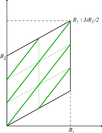
Figure 7.8: A (3,2) brane wrapping a tilted torus.

With these modifications in mind, we can then straightforwardly generalise our previous results for a Scherk-Schwarz deformation acting along the horizontal axis to the case of a tilted torus: once more, it is the parity of $\omega_{\alpha}$ to discriminate between a trivial or non-trivial action on the neutral non-chiral fermions.

7.4 Six-dimensional orbifold models

As a second application, we consider the non-supersymmetric type IIB string compactified on the $(T^{2}\times T^{2})/\mathbb{Z}_{2}$ with the Scherk-Schwarz deformation acting along the horizontal axis of the first $T^{2}$.

7.4.1 Preludio: the closed-string sector

In the Scherk-Schwarz basis, the torus partition function reads [93]

$$\mathcal{T} = {\textstyle{1\over 2}}\Biggl{[}\left(|V_{8}|^{2}+|S_{8}|^{2}\right)\,\Lambda_{2n_{1}}^{(4,4)}-\left(S_{8}\bar{V}_{8}+V_{8}\bar{S}_{8}\right)\,\Lambda^{(4,4)}_{m_{1}+{1\over 2},2n_{1}}+\left(|O_{8}|^{2}+|C_{8}|^{2}\right)\,\Lambda^{(4,4)}_{2n_{1}+1}$$ (7.18)

$$- \left(C_{8}\bar{O}_{8}+O_{8}\bar{C}_{8}\right)\,\Lambda^{(4,4)}_{m_{1}+{1\over 2},2n_{1}+1}+\left(|V_{4}O_{4}-O_{4}V_{4}|^{2}+|C_{4}C_{4}-S_{4}S_{4}|^{2}\right)\,\left|{2\eta\over\theta_{2}}\right|^{4}\Biggr{]}$$

$$+ {\textstyle{16\over 4}}\,\left[\left(|Q_{s}+Q_{c}|^{2}+|Q_{s}^{\prime}+Q_{c}^{\prime}|^{2}\right)\,\left|{\eta\over\theta_{4}}\right|^{4}+\left(|Q_{s}-Q_{c}|^{2}+|Q_{s}^{\prime}-Q_{c}^{\prime}|^{2}\right)\,\left|{\eta\over\theta_{3}}\right|^{4}\right]\,,$$

where $\Lambda^{(4,4)}$ is the four-dimensional Narain lattice with momenta $m_{1}\,,\ldots\,,m_{4}$ and windings $n_{1}\,,\ldots\,,n_{4}$. Moreover, $\Lambda_{2n_{1}}^{(4,4)}$ indicates that the winding number $n_{1}$ is now an even integer, and similarly for the other terms. The $Q$’s are defined as usual by

$$\eqalign{Q_{o}=&\,V_{4}O_{4}-C_{4}C_{4}\,,\cr Q_{v}=&\,O_{4}V_{4}-S_{4}S_{4}\,,\cr Q_{s}=&\,O_{4}C_{4}-S_{4}O_{4}\,,\cr Q_{c}=&\,V_{4}S_{4}-C_{4}V_{4}\,,\cr}\qquad\eqalign{Q_{o}^{\prime}=&\,V_{4}O_{4}-S_{4}S_{4}\,,\cr Q_{v}^{\prime}=&\,O_{4}V_{4}-C_{4}C_{4}\,,\cr Q_{s}^{\prime}=&\,O_{4}S_{4}-C_{4}O_{4}\,,\cr Q_{c}^{\prime}=&\,V_{4}C_{4}-S_{4}V_{4}\,,\cr}$$

where we have introduced additional $Q$’s that will play a role in the following. The Klein bottle amplitude obtained by the $\Omega\mathscr{R}(-1)^{F_{\rm L}}$ projection reads [93]

$$\eqalign{\mathcal{K}=&{\textstyle{1\over 4}}(V_{8}-S_{8})\left(P_{m}^{1}W_{n}^{2}P_{m}^{3}W_{n}^{4}+W_{2n}^{1}P_{m}^{2}W_{n}^{3}P_{m}^{4}\right)+{\textstyle{1\over 4}}(O_{8}-C_{8})\,W_{2n+1}^{1}P_{m}^{2}W_{n}^{3}P_{m}^{4}\cr&+4\left(Q_{s}+Q_{c}+Q_{s}^{\prime}+Q_{c}^{\prime}\right)\,\left({\eta\over\theta_{4}}\right)^{2}\,.\cr}$$

After an $S$-modular transformation to the transverse channel, and adapting to our six-dimensional example the definition in (7.8) , the massless contributions to the NS-NS and R-R tadpoles

$$\tilde{\mathcal{K}}_{0}\sim 8\,V_{4}O_{4}\,\left({\bf R}+{1\over{\bf R}}\right)^{2}+8\,O_{4}V_{4}\,\left({\bf R}-{1\over{\bf R}}\right)^{2}-8\,(C_{4}C_{4}+S_{4}S_{4})\,{\bf R}^{2}$$

clearly suggest that the O7-planes stretched along the vertical axis of the two $T^{2}$’s come in conjugate pairs and thus do not induce any R-R charge for the corresponding eight-form potential. The configuration of O7-planes stretched along the horizontal axis has instead a non-trivial charge that has to be compensated by suitable brane configurations [93]. Since we are altering the nature of some orientifold planes, we cannot expect that the new open-string spectrum might be obtained from the undeformed one by giving masses to the fermions in the adjoint of the $U(N_{i})$ gauge group factors. In fact, this configuration would not solve any longer the untwisted R-R tadpole conditions, and thus new vacuum configurations have to be found.

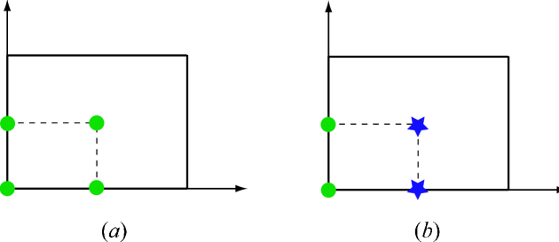
Figure 7.9: Fixed points for a $\mathbb{Z}_{2}$ orbifold without $(a)$ and with $(b)$ Scherk-Schwarz deformation.

Before we proceed with the construction of the open-string sector, let us pause for a moment and try to extract some useful information about the geometry of this Scherk-Schwarz-deformed $T^{4}/\mathbb{Z}_{2}$. To this end it is convenient to stare at the twisted sector in (7.18). The appearance of new characters $Q_{s,c}^{\prime}$ and the modified multiplicity clearly spells out that the original sixteen fixed points of the geometrical $\mathbb{Z}_{2}$ orbifold model are now split into two sets of eight, with different GSO projections in the corresponding twisted sector. Moreover, one can also read from the terms $Q_{s}-Q_{c}$ and $Q_{s}^{\prime}-Q_{c}^{\prime}$ that the fixed points act differently on the internal quantum numbers. Indeed, if we call $\xi_{\mu}$ and $x_{\mu}$ ($\mu=1,\ldots,8$) the fixed points in the two sets, the eight $\xi_{\mu}$ project the spectrum with respect the geometrical $\mathbb{Z}_{2}$ while the eight $x_{\mu}$ involve also the action of the Scherk-Schwarz deformation $(-1)^{F}$, for an overall $g\,(-1)^{F}$ projection, $g$ being the $\mathbb{Z}_{2}$ generator. This is clear both from the kind of boundary conditions we are imposing and from the structure of the modular-invariant partition function, where the projection in $Q_{s}^{\prime}-Q_{c}^{\prime}$ involves and additional $(-1)^{F}$ with respect to that in $Q_{s}-Q_{c}$. We can actually say more about the geometrical distribution of these fixed points. In our factorised $T^{4}=T^{2}\times T^{2}$ example, in fact, we have chosen to impose Scherk-Schwarz boundary conditions along the horizontal axis of the first torus. As a result, the structure of the fixed points in the second torus cannot be affected. In the first torus, instead, we have the configuration depicted in figure 9, since, as previously reminded, we are deforming the theory by changing the boundary conditions along the horizontal axis. Therefore, we can conclude that our $T^{4}$ is of the form $T^{2}_{(b)}\times T^{2}_{(a)}$, where $T^{2}_{(a)}$ and $T^{2}_{(b)}$ denote the undeformed and the deformed torus as in figure 7.9. The two sets of fixed points are then

$$\vec{\xi} = \bigg{\{}(0,0,0,0),(0,0,{\textstyle{1\over 2}},0),(0,0,0,{\textstyle{1\over 2}}),(0,0,{\textstyle{1\over 2}},{\textstyle{1\over 2}}),$$

$$(0,{\textstyle{1\over 2}},0,0),(0,{\textstyle{1\over 2}},{\textstyle{1\over 2}},0),(0,{\textstyle{1\over 2}},0,{\textstyle{1\over 2}}),(0,{\textstyle{1\over 2}},{\textstyle{1\over 2}},{\textstyle{1\over 2}})\bigg{\}}\,,$$

$$\vec{x} = \bigg{\{}({\textstyle{1\over 2}},0,0,0),({\textstyle{1\over 2}},0,{\textstyle{1\over 2}},0),({\textstyle{1\over 2}},0,0,{\textstyle{1\over 2}}),({\textstyle{1\over 2}},0,{\textstyle{1\over 2}},{\textstyle{1\over 2}}),$$ (7.19)

$$({\textstyle{1\over 2}},{\textstyle{1\over 2}},0,0),({\textstyle{1\over 2}},{\textstyle{1\over 2}},{\textstyle{1\over 2}},0),({\textstyle{1\over 2}},{\textstyle{1\over 2}},0,{\textstyle{1\over 2}}),({\textstyle{1\over 2}},{\textstyle{1\over 2}},{\textstyle{1\over 2}},{\textstyle{1\over 2}})\bigg{\}}\,.$$

7.4.2 Intermezzo: the geometry of orthogonal branes

We can now proceed to include the D-branes, and to better appreciate the construction of the open-string sector we first review the model presented in [93], with the obvious replacement of D9 and D5 with two sets of orthogonal D7 branes. To reproduce their geometry we distribute the branes as in figure 7.10, that, after two T-dualities along the vertical axis of the two $T^{2}$’s correspond indeed to space-filling D9 branes together with a set of D5 branes sitting at the fixed point $\xi_{1}=(0,0,0,0)$ and a set of D5 anti-branes sitting at the fixed point $x_{1}=({1\over 2},0,0,0)$.

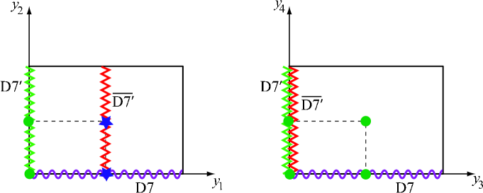
Figure 7.10: The geometry of D-branes. A wavy line represents D7 branes while zig-zag lines represents ${\rm D}7^{\prime}$ and $\overline{{\rm D}7^{\prime}}$.

The direct-channel annulus in [93] is then

$$\eqalign{\mathcal{A}=&{\textstyle{1\over 4}}\Biggl{\{}N_{7}^{2}\left(V_{8}\,P^{1}_{m}-S_{8}\,P^{1}_{m+{1\over 2}}\right)W^{2}_{n}P^{3}_{m}W^{4}_{n}+\left(N_{7^{\prime}}^{2}+N_{\overline{7^{\prime}}}^{2}\right)(Q_{o}+Q_{v})\,W_{n}^{1}P_{m}^{2}W_{n}^{3}P_{m}^{4}\cr&+2N_{7^{\prime}}N_{\overline{7^{\prime}}}\,(O_{8}-C_{8})W^{1}_{n+{1\over 2}}P^{2}_{m}W^{3}_{n}P^{4}_{m}+R^{2}_{7}\,(V_{4}O_{4}-O_{4}V_{4})\left({2\eta\over\theta_{2}}\right)^{2}\cr&+\left[R_{7^{\prime}}^{2}(Q_{o}-Q_{v})+R_{\overline{7^{\prime}}}^{2}(Q_{o}^{\prime}-Q_{v}^{\prime})\right]\left({2\eta\over\theta_{2}}\right)^{2}\cr&+2\left[N_{7}N_{7^{\prime}}\,(Q_{s}+Q_{c})+N_{7}N_{\overline{7^{\prime}}}(Q_{s}^{\prime}+Q_{c}^{\prime})\right]\left({\eta\over\theta_{4}}\right)^{2}\cr&+2\left[R_{7}R_{7^{\prime}}(Q_{s}-Q_{c})+R_{7}R_{\overline{7^{\prime}}}(Q_{s}^{\prime}-Q_{c}^{\prime})\right]\left({\eta\over\theta_{3}}\right)^{2}\Biggr{\}}\,.\cr}$$

Any single term in this expression has a clear rational. The terms in the first line simply correspond to open strings living on a given D-brane, with the important difference that D7 branes stretching along the horizontal $y_{1}$ axis now have a deformed non-supersymmetric spectrum. The second line is also quite standard: the first term encodes the spectrum of a brane-anti-brane system with the two ${\rm D}7^{\prime}$ and $\overline{D7^{\prime}}$ branes separated along $y_{1}$, while the second contribution pertains to the orbifold projection on the horizontal D7 branes. Also the fourth line is quite standard: it corresponds to open strings with mixed Neumann-Dirichlet boundary conditions along the four-compact directions. The second term has different GSO projections since the strings stretch between a brane and an anti-brane. More subtle are the third and fifth lines. They both enforce the orbifold projection on open-strings, but in a different way. In fact, while the first term in the third line clearly corresponds to the conventional geometrical $\mathbb{Z}_{2}$ projection, the second term involves and additional minus sign in the Ramond sector, and indeed corresponds to the action of the element $g(-1)^{F}$. This is consistent with, and in fact dictated by, the fact that ${\rm D}7^{\prime}$ branes sit on top of conventional $g$-fixed points, while the $\overline{{\rm D}7^{\prime}}$ branes pass through points fixed under the action of $g(-1)^{F}$. Clearly, similar considerations also apply to the terms in the fifth line that describe the symmetrisation of $7\,7^{\prime}$ and $7\,\overline{7^{\prime}}$ states that indeed live at the fixed points $\xi_{1}$ and $x_{1}$. As usual, the different orbifold projections in the direct channel translate into exchanges of closed-string twisted states in the transverse channel, whose massless tadpoles clearly spell out the distribution of branes among the fixed points

$$\tilde{\mathcal{A}}_{\rm tw}\sim 2^{-5}\,\left\{\left[\left(R_{7}-R_{7^{\prime}}\right)^{2}+R^{2}_{7}+3\,R^{2}_{7^{\prime}}\right]\,Q_{s}+\left[\left(R_{7}-R_{\overline{7^{\prime}}}\right)^{2}+R^{2}_{7}+3\,R^{2}_{\overline{7^{\prime}}}\right]\,Q_{s}^{\prime}\right\}\,,$$

compatible with the geometry in figure 7.10.

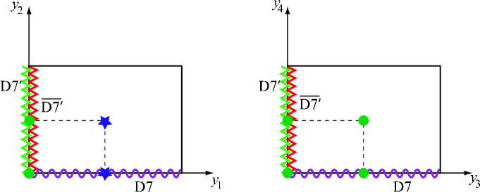
Figure 7.11: The geometry of D-branes. A wavy line represents D7 branes while zig-zag lines represents ${\rm D}7^{\prime}$ and $\overline{{\rm D}7^{\prime}}$.

What about if we distribute branes differently? Let us consider for instance the configuration in figure 7.11. Now all the branes pass through the conventional $g$-fixed points, and thus we do not expect in the amplitude terms like $Q_{o}^{\prime}-Q_{v}^{\prime}$. Indeed, the new annulus amplitude

$$\eqalign{\mathcal{A}=&{\textstyle{1\over 4}}\Biggl{\{}N_{7}^{2}\,\left(V_{8}\,P^{1}_{m}-S_{8}\,P^{1}_{m+{1\over 2}}\right)W^{2}_{n}P^{3}_{m}W^{4}_{n}+\left(N_{7^{\prime}}^{2}+N_{\overline{7^{\prime}}}^{2}\right)(Q_{o}+Q_{v})\,W^{1}_{n}P^{2}_{m}W^{3}_{n}P^{4}_{m}\cr&+2N_{7^{\prime}}N_{\overline{7^{\prime}}}\,(O_{8}-C_{8})\,W^{1}_{n}P^{2}_{m}W^{3}_{n}P^{4}_{m}+R_{7}^{2}\,(V_{4}O_{4}-O_{4}V_{4})\left({2\eta\over\theta_{2}}\right)^{2}\cr&+\left[\left(R_{7^{\prime}}^{2}+R_{\overline{7^{\prime}}}^{2}\right)(Q_{o}-Q_{v})+2R_{7^{\prime}}R_{\overline{7^{\prime}}}\,(O_{4}O_{4}-V_{4}V_{4}-S_{4}C_{4}+C_{4}S_{4})\right]\left({2\eta\over\theta_{2}}\right)^{2}\cr&+2\left[N_{7}N_{7^{\prime}}\,(Q_{s}+Q_{c})+N_{7}N_{\overline{7^{\prime}}}\,(Q_{s}^{\prime}+Q_{c}^{\prime})\right]\left({\eta\over\theta_{4}}\right)^{2}\cr&+2\left[R_{7}R_{7^{\prime}}\,(Q_{s}-Q_{c})+R_{7}R_{\overline{7^{\prime}}}\,(-O_{4}S_{4}+V_{4}C_{4}-C_{4}O_{4}+S_{4}V_{4})\right]\left({\eta\over\theta_{3}}\right)^{2}\cr}$$

only involves the geometrical $\mathbb{Z}_{2}$ projector, and yields twisted tadpoles in the transverse channel

$$\eqalign{\tilde{\mathcal{A}}_{\rm tw}\sim&2^{-5}\left\{2R^{2}_{7}\,Q_{s}^{\prime}+\left[\left(R_{7}-R_{7^{\prime}}+R_{\overline{7^{\prime}}}\right)^{2}+R^{2}_{7}+3(R_{7^{\prime}}-R_{\overline{7^{\prime}}})^{2}\right]\,O_{4}C_{4}\right.\cr&-\left.\left[\left(R_{7}-R_{7^{\prime}}-R_{\overline{7^{\prime}}}\right)^{2}+R^{2}_{7}+3(R_{7^{\prime}}+R_{\overline{7^{\prime}}})^{2}\right]\,S_{4}O_{4}\right\}\cr}$$

that clearly display the distribution in figure 7.11.

Similarly, one could opt for a different distribution of branes along the compact $T^{4}$, that would consequently imply different projections according to the nature of the fixed points crossed by the branes. This would then reflect in twisted tadpoles compatible with the chosen geometry.

7.4.3 Crescendo: rotating the branes

We can now generalise the previous construction to the case of rotated branes, where some care is needed to identify the exact location of brane intersections. In the simple case where all branes cross the origin of the two tori, it was shown in [133] that any brane always passes through four fixed points of the $T^{4}/\mathbb{Z}_{2}$. Moreover, we can easily identify the four points from the wrapping numbers $(\omega_{\alpha}^{\Lambda},\kappa_{\alpha}^{\Lambda})$, since for a single $T^{2}$ branes fall into three different equivalence classes: $\omega_{\alpha}$ even and $\kappa_{\alpha}$ odd, $\omega_{\alpha}$ odd and $\kappa_{\alpha}$ even, $\omega_{\alpha}$ and $\kappa_{\alpha}$ both odd and co-prime. Focussing our attention to the first $T^{2}$, the only one that actually matters to identify the correct projection, one has then the cases reported in figure 7.12.

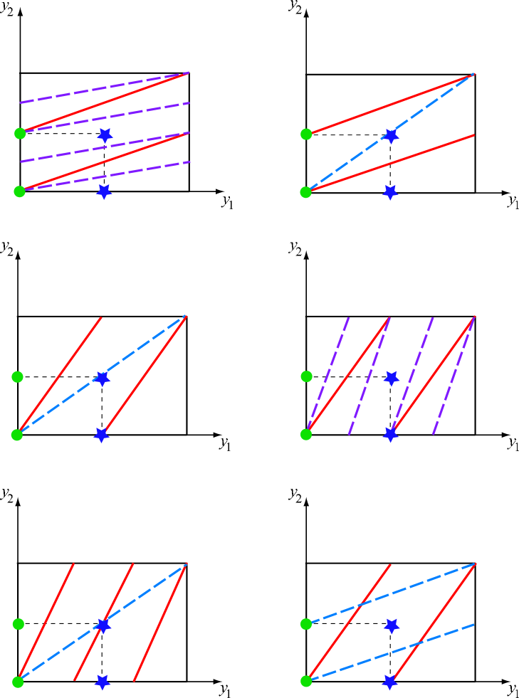
Figure 7.12: Branes with various wrapping numbers on a $(b)$ torus.

The annulus amplitude associated to the closed-string sector in sub-section 7.4.1 is then

$$\eqalign{\mathcal{A}_{\alpha\alpha}=&{\textstyle{1\over 2}}\sum_{a=1}^{m_{\rm e}}N_{a}\bar{N}_{a}\,(Q_{o}+Q_{v})[{\textstyle{0\atop 0}}]\,P_{m}^{1}W_{n}^{1}P_{m}^{2}W_{n}^{2}+{\textstyle{1\over 2}}\sum_{a=1}^{m_{\rm e}}N_{a}\bar{N}_{a}\,(Q_{o}-Q_{v})[{\textstyle{0\atop 0}}]\,{4\over\Upsilon_{2}[{\textstyle{0\atop 0}}]}\cr&+{\textstyle{1\over 2}}\sum_{i=1}^{m_{\rm o}}N_{i}\bar{N}_{i}\,\left(V_{8}[{\textstyle{0\atop 0}}]\,P_{m}^{1}-S_{8}[{\textstyle{0\atop 0}}]\,P_{m+{1\over 2}}^{1}\right)W_{n}^{1}P_{m}^{2}W_{n}^{2}\cr&+{\textstyle{1\over 2}}\sum_{i=1}^{m_{\rm o}}N_{i}\bar{N}_{i}\,(V_{4}O_{4}-O_{4}V_{4})[{\textstyle{0\atop 0}}]\,{4\over\Upsilon_{2}[{\textstyle{0\atop 0}}]}\,,\cr}$$

$$\eqalign{\mathcal{A}_{\alpha\bar{\alpha}}+\mathcal{A}_{\bar{\alpha}\alpha}=&{\textstyle{1\over 4}}\sum_{\alpha=1}^{m_{\rm o}+m_{\rm e}}\left(N_{\alpha}^{2}(Q_{o}+Q_{v})[{\textstyle{\alpha\bar{\alpha}\atop 0}}]+\bar{N}_{\alpha}^{2}(Q_{o}+Q_{v})[{\textstyle{\bar{\alpha}\alpha\atop 0}}]\right)\,{I_{\alpha\bar{\alpha}}\over\Upsilon_{1}[{\textstyle{\alpha\bar{\alpha}\atop 0}}]}\cr&-{\textstyle{1\over 4}}\sum_{a=1}^{m_{\rm e}}\left(N_{a}^{2}(Q_{o}-Q_{v})[{\textstyle{a\bar{a}\atop 0}}]+\bar{N}_{a}^{2}(Q_{o}-Q_{v})[{\textstyle{\bar{a}a\atop 0}}]\right)\,{4\over\Upsilon_{2}[{\textstyle{a\bar{a}\atop 0}}]}\cr&-{\textstyle{1\over 4}}\sum_{i=1}^{m_{\rm o}}\left(N_{i}^{2}(Q_{o}-Q_{v})[{\textstyle{i\bar{\imath}\atop 0}}]+\bar{N}_{i}^{2}(Q_{o}-Q_{v})[{\textstyle{\bar{\imath}i\atop 0}}]\right)\,{2\over\Upsilon_{2}[{\textstyle{i\bar{\imath}\atop 0}}]}\cr&-{\textstyle{1\over 4}}\sum_{i=1}^{m_{\rm o}}\left(N_{i}^{2}(Q_{o}^{\prime}-Q_{v}^{\prime})[{\textstyle{i\bar{\imath}\atop 0}}]+\bar{N}_{i}^{2}(Q_{o}^{\prime}-Q_{v}^{\prime})[{\textstyle{\bar{\imath}i\atop 0}}]\right)\,{2\over\Upsilon_{2}[{\textstyle{i\bar{\imath}\atop 0}}]}\,,\cr}$$

$$\eqalign{\mathcal{A}_{\alpha\beta}+\mathcal{A}_{\bar{\alpha}\bar{\beta}}=&{\textstyle{1\over 2}}\sum_{{\alpha,\beta=1\atop\beta<\alpha}}^{m_{\rm o}+m_{\rm e}}\left(N_{\alpha}\bar{N}_{\beta}(Q_{o}+Q_{v})[{\textstyle{\alpha\beta\atop 0}}]+\bar{N}_{\alpha}N_{\beta}(Q_{o}+Q_{v})[{\textstyle{\bar{\alpha}\bar{\beta}\atop 0}}]\right)\,{I_{\alpha\beta}\over\Upsilon_{1}[{\textstyle{\alpha\beta\atop 0}}]}\cr&+{\textstyle{1\over 2}}\sum_{{a,b=1\atop b<a}}^{m_{\rm e}}\left(N_{a}\bar{N}_{b}(Q_{o}-Q_{v})[{\textstyle{ab\atop 0}}]+\bar{N}_{a}N_{b}(Q_{o}-Q_{v})[{\textstyle{\bar{a}\bar{b}\atop 0}}]\right)\,{2I_{ab}^{\prime}\over\Upsilon_{2}[{\textstyle{ab\atop 0}}]}\cr&+{\textstyle{1\over 2}}\sum_{a=1}^{m_{\rm e}}\sum_{i=1}^{m_{\rm o}}\left(N_{a}\bar{N}_{i}(Q_{o}-Q_{v})[{\textstyle{ai\atop 0}}]+\bar{N}_{a}N_{i}(Q_{o}-Q_{v})[{\textstyle{\bar{a}\bar{\imath}\atop 0}}]\right)\,{I_{ai}^{\prime}\over\Upsilon_{2}[{\textstyle{ai\atop 0}}]}\cr&+{\textstyle{1\over 2}}\sum_{{i,j=1\atop j<i}}^{m_{\rm o}}\left(N_{i}\bar{N}_{j}(Q_{o}-Q_{v})[{\textstyle{ij\atop 0}}]+\bar{N}_{i}N_{j}(Q_{o}-Q_{v})[{\textstyle{\bar{\imath}\bar{\jmath}\atop 0}}]\right)\,{I_{ij}^{\prime}\over\Upsilon_{2}[{\textstyle{ij\atop 0}}]}\cr&+{\textstyle{1\over 2}}\sum_{{i,j=1\atop j<i}}^{m_{\rm o}}\left(N_{i}\bar{N}_{j}(Q_{o}^{\prime}-Q_{v}^{\prime})[{\textstyle{ij\atop 0}}]+\bar{N}_{i}N_{j}(Q_{o}^{\prime}-Q_{v}^{\prime})[{\textstyle{\bar{\imath}\bar{\jmath}\atop 0}}]\right)\,{I_{ij}^{\prime\prime}\over\Upsilon_{2}[{\textstyle{ij\atop 0}}]}\,,\cr}$$

and, finally,

$$\eqalign{\mathcal{A}_{\alpha\bar{\beta}}+\mathcal{A}_{\bar{\alpha}\beta}=&{\textstyle{1\over 2}}\sum_{{\alpha,\beta=1\atop\beta<\alpha}}^{m_{\rm o}+m_{\rm e}}\left(N_{\alpha}N_{\beta}(Q_{o}+Q_{v})[{\textstyle{\alpha\bar{\beta}\atop 0}}]+\bar{N}_{\alpha}\bar{N}_{\beta}(Q_{o}+Q_{v})[{\textstyle{\bar{\alpha}\beta\atop 0}}]\right)\,{I_{\alpha\bar{\beta}}\over\Upsilon_{1}[{\textstyle{\alpha\bar{\beta}\atop 0}}]}\cr&-{\textstyle{1\over 2}}\sum_{{a,b=1\atop b<a}}^{m_{\rm e}}\left(N_{a}N_{b}(Q_{o}-Q_{v})[{\textstyle{a\bar{b}\atop 0}}]+\bar{N}_{a}\bar{N}_{b}(Q_{o}-Q_{v})[{\textstyle{\bar{a}b\atop 0}}]\right)\,{2I_{a\bar{b}}^{\prime}\over\Upsilon_{2}[{\textstyle{a\bar{b}\atop 0}}]}\cr&-{\textstyle{1\over 2}}\sum_{a=1}^{m_{\rm e}}\sum_{i=1}^{m_{\rm o}}\left(N_{a}N_{i}(Q_{o}-Q_{v})[{\textstyle{a\bar{\imath}\atop 0}}]+\bar{N}_{a}\bar{N}_{i}(Q_{o}-Q_{v})[{\textstyle{\bar{a}i\atop 0}}]\right)\,{I_{a\bar{\imath}}^{\prime}\over\Upsilon_{2}[{\textstyle{a\bar{\imath}\atop 0}}]}\cr&-{\textstyle{1\over 2}}\sum_{{i,j=1\atop j<i}}^{m_{\rm o}}\left(N_{i}N_{j}(Q_{o}-Q_{v})[{\textstyle{i\bar{\jmath}\atop 0}}]+\bar{N}_{i}\bar{N}_{j}(Q_{o}-Q_{v})[{\textstyle{\bar{\imath}j\atop 0}}]\right)\,{I_{i\bar{\jmath}}^{\prime}\over\Upsilon_{2}[{\textstyle{i\bar{\jmath}\atop 0}}]}\cr&-{\textstyle{1\over 2}}\sum_{{i,j=1\atop j<i}}^{m_{\rm o}}\left(N_{i}N_{j}(Q_{o}^{\prime}-Q_{v}^{\prime})[{\textstyle{i\bar{\jmath}\atop 0}}]+\bar{N}_{i}\bar{N}_{j}(Q_{o}^{\prime}-Q_{v}^{\prime})[{\textstyle{\bar{\imath}j\atop 0}}]\right)\,{I_{i\bar{\jmath}}^{\prime\prime}\over\Upsilon_{2}[{\textstyle{i\bar{\jmath}\atop 0}}]}\,.\cr}$$

Here we have used the obvious notation for the $Q[{\alpha\beta\atop\gamma\delta}]$ where the internal $SO(4)$ characters are decomposed in terms of $SO(2)\times SO(2)$ ones, and

$$\Upsilon_{2}[{\textstyle{\alpha\beta\atop\gamma\delta}}]=\prod_{\Lambda=1,2}\,{\theta_{2}(\zeta^{\Lambda}|\tau)\over\eta(\tau)}\,e^{2i\pi\zeta^{\Lambda}}\,,$$

accounts for the $\mathbb{Z}_{2}$ orbifold generator acting on the world-sheet bosons. Finally, $I_{\alpha\beta}$ denotes as usual the number of intersections of branes with wrapping numbers $(\omega_{\alpha}^{\Lambda}\,,\,\kappa_{\alpha}^{\Lambda})$ and $(\omega_{\beta}^{\Lambda}\,,\,\kappa_{\beta}^{\Lambda})$, while

$$I^{\prime}_{\alpha\beta}=1+\Pi(\omega_{\alpha}^{2}-\omega_{\beta}^{2})\,\Pi(\kappa_{\alpha}^{2}-\kappa_{\beta}^{2})$$

and

$$I^{\prime\prime}_{\alpha\beta}=\Pi(\omega_{\alpha}^{1}+1)\Pi(\omega_{\beta}^{1}+1)\,\Pi(\kappa_{\alpha}^{1}-\kappa_{\beta}^{1})\,I^{\prime}_{\alpha\beta}$$

count the number of intersections that actually coincide with the $x_{p}$ and $\xi_{p}$ fixed points in (7.4.1), with

$$\Pi(\mu)={\textstyle{1\over 2}}\sum_{\epsilon=0,1}e^{i\pi\epsilon\mu}\,,\qquad\mu\in\mathbb{Z}\,,$$

a $\mathbb{Z}_{2}$ projector.

Finally, the Möbius-strip amplitude

$$\mathcal{M} = -{\textstyle{1\over 4}}\sum_{\alpha=1}^{m_{\rm o}+m_{\rm e}}\,\big{[}\left(N_{\alpha}\,(\hat{Q}_{o}+\hat{Q}_{v})[{\textstyle{\alpha\bar{\alpha}\atop 0}}]+\bar{N}_{\alpha}\,(\hat{Q}_{o}+\hat{Q}_{v})[{\textstyle{\bar{\alpha}\alpha\atop 0}}]\right)\,{K_{\alpha}\over\hat{\Upsilon}_{1}[{\textstyle{\alpha\bar{\alpha}\atop 0}}]}$$ (7.20)

$$- \left(N_{\alpha}\,(\hat{V}_{4}\hat{O}_{4}-\hat{O}_{4}\hat{V}_{4})[{\textstyle{\alpha\bar{\alpha}\atop 0}}]+\bar{N}_{\alpha}\,(\hat{V}_{4}\hat{O}_{4}-\hat{O}_{4}\hat{V}_{4})[{\textstyle{\bar{\alpha}\alpha\atop 0}}]\right)\,{J_{\alpha}\over\hat{\Upsilon}_{2}[{\textstyle{\alpha\bar{\alpha}\atop 0}}]}\big{]}$$

takes now into account also the (anti-)symmetrisation of states that live at intersections sitting on the vertical O7 planes, whose number is given by

$$J_{\alpha}=\prod_{\Lambda=1,2}\,2\,\omega_{\alpha}^{\Lambda}\,.$$

Notice that the second line in $\mathcal{M}$ does not involve fermions. This has a simple explanation in terms of the relative R-R charges of vertical O-planes and branes whose intersections lie on them. We already commented that the absence in $\tilde{\mathcal{K}}_{0}$ of R-R tadpoles proportional to ${\bf R}^{-1}$ clearly spells out that the O7 planes passing through the points $(0,0)$ and $({1\over 2}R_{1},0)$ and extending along the vertical direction are conjugates pairs. This implies that their R-R charges are equal and opposite. On the other hand the branes have positive R-R charge, and thus fermions localised at the intersections sitting on the O7 plane are (say) symmetrised while those sitting on the O7 anti-planes (equal in number) are anti-symmetrised. As a result, their net contributions to $\mathcal{M}$ is zero, consistently with the expression (7.20).

After $S$ and $P$ modular transformations to the tree-level channel the low-lying untwisted states in $\tilde{\mathcal{K}}$, $\tilde{\mathcal{A}}$ and $\tilde{\mathcal{M}}$ yield the familiar conditions

$$\sum_{\alpha=1}^{m_{\rm e}+m_{\rm o}}\,{\bf L}_{\alpha}\,\left(N_{\alpha}+\bar{N}_{\alpha}\right)=32\left({\bf R}+{1\over{\bf R}}\right)$$

for the NS-NS dilaton tadpole, and

$$\sum_{\alpha=1}^{m_{\rm e}+m_{\rm o}}\,{\bf L}_{\alpha}\,\left(N_{\alpha}\,e^{2i\phi_{\alpha}\cdot\eta}+\bar{N}_{\alpha}\,e^{-2i\phi_{\alpha}\cdot\eta}\right)=32\,{\bf R}$$

for the R-R tadpole with, as usual, $\eta^{\Lambda}$ the chirality of the internal spinors. In both expressions ${\bf L}_{\alpha}$ and ${\bf R}$ are defined as in (7.8) , with $\Lambda=1,2$ running now over the two $T^{2}$’s.

Much more interesting are the twisted tadpoles since, as repeatedly stated in the previous sub-sections, they clearly display the geometry of the brane configuration. After an $S$ modular transformation one then gets the massless tadpoles

$$C_{4}O_{4}\,:\quad\sum_{i=1}^{m_{\rm o}}\,\left(N_{i}-\bar{N}_{i}\right)\,P(z_{p}\in D_{i})=0\,,\qquad\forall\,z_{p}\in\{x\}\,,$$ (7.21)

and

$$S_{4}O_{4}\,:\quad\sum_{a=1}^{m_{\rm e}}\,(N_{a}-\bar{N}_{a})\,P(z_{q}\in D_{a})+\sum_{i=1}^{m_{\rm o}}\,(N_{i}-\bar{N}_{i})\,P(z_{q}\in D_{i})=0\,,\qquad\forall\,z_{q}\in\{\xi\}$$ (7.22)

where $D_{\alpha}$ denotes the straight line drawn by the $\alpha$-th brane with wrapping numbers $(\omega^{\Lambda}_{\alpha},\kappa^{\Lambda}_{\alpha})$, and

$$P(w_{\ell}\in D_{\alpha})=\cases{1&if $w_{\ell}\in D_{\alpha}$\cr 0&if $w_{\ell}\not\in D_{\alpha}$\cr}$$

equals one or vanishes depending on whether the point $w_{\ell}$ belongs to the line $D_{\alpha}$ or does not. In the simple case where all branes pass through the origin, the $P(w_{\ell}\in D_{\alpha})$ are collected in tables (7.5) and (7.6).

$z_{p}$	$P(z_{p}\in D_{i})$
$x_{1}$	$\Pi(\kappa^{1}_{i})\,\Pi(\omega^{1}_{i}+1)$
$x_{2}$	$\Pi(\kappa^{1}_{i})\,\Pi(\omega^{1}_{i}+1)\,\Pi(\kappa^{2}_{i})\,\Pi(\omega^{2}_{i}+1)$
$x_{3}$	$\Pi(\kappa^{1}_{i})\,\Pi(\omega^{1}_{i}+1)\,\Pi(\kappa^{2}_{i}+1)\,\Pi(\omega^{2}_{i})$
$x_{4}$	$\Pi(\kappa^{1}_{i})\,\Pi(\omega^{1}_{i}+1)\,\Pi(\kappa^{2}_{i}+1)\,\Pi(\omega^{2}_{i}+1)$
$x_{5}$	$\Pi(\kappa^{1}_{i}+1)\,\Pi(\omega^{1}_{i}+1)$
$x_{6}$	$\Pi(\kappa^{1}_{i}+1)\,\Pi(\omega^{1}_{i}+1)\,\Pi(\kappa^{2}_{i})\,\Pi(\omega^{2}_{i}+1)$
$x_{7}$	$\Pi(\kappa^{1}_{i}+1)\,\Pi(\omega^{1}_{i}+1)\,\Pi(\kappa^{2}_{i}+1)\,\Pi(\omega^{2}_{i})$
$x_{8}$	$\Pi(\kappa^{1}_{i}+1)\,\Pi(\omega^{1}_{i}+1)\,\Pi(\kappa^{2}_{i}+1)\,\Pi(\omega^{2}_{i}+1)$

Table 7.5: Condition for the $\alpha$-th brane to pass through the fixed point $x_{p}$.

Turning to the twisted NS-NS tadpoles, they can be easily deduced from (7.21) and (7.22) and from their analogy with the untwisted R-R tadpoles. Denoting as usual by $\eta^{\Lambda}=\pm{1\over 2}$ the chirality of the internal $SO(2)$ spinors, one finds

$$\eqalign{O_{4}S_{4}\,:&\sum_{i=1}^{m_{\rm o}}\,\left(N_{i}\,e^{2i\phi_{i}\cdot\eta}-\bar{N}_{i}\,e^{2i\phi_{i}\cdot\eta}\right)\,P(z_{p}\in D_{i})\cr\sim&\sum_{i=1}^{m_{\rm o}}\,N_{i}\,\sin(2\phi_{i}\cdot\eta)\,P(z_{p}\in D_{i})\,,\qquad\forall\,z_{p}\in\{x\}\cr}$$

and, similarly

$$O_{4}C_{4}\,:\quad\sum_{a=1}^{m_{\rm e}}\,N_{a}\,\sin(2\phi_{a}\cdot\eta)\,P(z_{q}\in D_{a})+\sum_{i=1}^{m_{\rm o}}\,N_{i}\,\sin(2\phi_{i}\cdot\eta)\,P(z_{q}\in D_{i})\,,\quad\forall\,z_{q}\in\{\xi\}\,.$$

As expected, in non-supersymmetric models these tadpoles cannot be imposed to vanish, and yield additional contributions to the low-energy effective action [112].

Also in this case, additional non-chiral fermions originating from branes that are parallel in the second $T^{2}$ can be made massive if a Scherk-Schwarz deformation is acting also in this torus. In this case, however, one is consequently reshuffling the fixed points in the two sets $\xi$ and $x$ and thus some care is needed in determining the correct spectrum of the brane intersections.

$z_{q}$	$P(z_{q}\in D_{i})$
$\xi_{1}$	1
$\xi_{2}$	$\Pi(\kappa^{2}_{\alpha})\,\Pi(\omega^{2}_{\alpha}+1)$
$\xi_{3}$	$\Pi(\kappa^{2}_{\alpha}+1)\,\Pi(\omega^{2}_{\alpha})$
$\xi_{4}$	$\Pi(\kappa^{2}_{\alpha}+1)\,\Pi(\omega^{2}_{\alpha}+1)$
$\xi_{5}$	$\Pi(\kappa^{1}_{a}+1)\,\Pi(\omega^{1}_{a})$
$\xi_{6}$	$\Pi(\kappa^{1}_{a}+1)\,\Pi(\omega^{1}_{a})\,\Pi(\kappa^{2}_{a})\,\Pi(\omega^{2}_{a}+1)$
$\xi_{7}$	$\Pi(\kappa^{1}_{a}+1)\,\Pi(\omega^{1}_{a})\,\Pi(\kappa^{2}_{a}+1)\,\Pi(\omega^{2}_{a})$
$\xi_{8}$	$\Pi(\kappa^{1}_{a}+1)\,\Pi(\omega^{1}_{a})\,\Pi(\kappa^{2}_{a}+1)\,\Pi(\omega^{2}_{a}+1)$

Table 7.6: Condition for the $\alpha$-th brane to pass through the fixed point $\xi_{q}$.

7.4.4 Finale: an interesting example

To conclude with this deformed $T^{4}/\mathbb{Z}_{2}$ compactification let us present a simple solution to tadpole conditions. We consider three sets of $N_{\alpha}$ coincident branes with wrapping numbers

$$(\omega^{\Lambda}_{1},\kappa^{\Lambda}_{1})=\left(\matrix{(1,0)\cr(1,1)\cr}\right)\,,\quad(\omega^{\Lambda}_{2},\kappa^{\Lambda}_{2})=\left(\matrix{(2,1)\cr(0,1)\cr}\right)\,,\quad(\omega^{\Lambda}_{3},\kappa^{\Lambda}_{3})=\left(\matrix{(1,2)\cr(1,-1)\cr}\right)\,,$$ (7.23)

as depicted in figure 13. These numbers, together with the choice $N_{1}=10$, $N_{2}=12$ and $N_{3}=6$ clearly satisfy the R-R tadpole conditions.

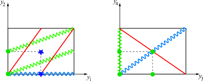
Figure 7.13: A simple example with three sets of branes.

At the level of toroidal compactification (i.e. before we mod out by the orbifold action and before we deform the spectrum à la Scherk-Schwarz) the chiral spectrum comprises left-handed fermions in the representation $2\,(10,12,1)+5\,(1,12,6)+4\,(1,66,1)$ together with right-handed fermions in the representation $4\,(10,1,6)+3\,(1,12,6)+8\,(1,1,15)+2\,(1,66,1)+2\,(1,78,1)$, and is clearly free of any irreducible gravitational and gauge anomaly. Before we project and deform the spectrum, let us comment about one subtlety that one meets in deriving this chiral spectrum. In particular, from table 7.7 one would naively deduce that the $2\,\bar{2}$ sector is non-chiral since the corresponding intersection number is zero. However, since $K_{2}=4\not=0$, there is a non-vanishing $N_{2}$-contribution in the Möbius strip amplitude that apparently is not matched by the annulus. This is evidently not the case and the correct interpretation is as follows: despite the $N_{2}$ branes and their images are parallel in the second $T^{2}$ they intersect non-trivially in the first torus. Moreover, the non-chirality of the annulus suggests that left-handed fermions live at four intersections, and similarly do the right-handed ones, while the “chirality” of the Möbius clearly states that only the left-handed fermions lie on top of the orientifold planes. As a result, one gets four copies of left-handed spinors in the antisymmetric representation of $U(12)$ together with two copies of right-handed spinors in the symmetric plus antisymmetric representations.

$\alpha\beta$		$I_{\alpha\beta}$		$I^{\prime}_{\alpha\beta}$		$I^{\prime\prime}_{\alpha\beta}$
$12$		$1$		$1$		$0$
$13$		$-4$		$2$		$2$
$23$		$-3$		$1$		$0$
$1\bar{2}$		$1$		$1$		$0$
$1\bar{3}$		$0$		$2$		$2$
$2\bar{3}$		$5$		$1$		$0$
$1\bar{1}$		$0$		$2$		$0$
$2\bar{2}$		$0$		$2$		$0$
$3\bar{3}$		$-8$		$2$		$2$

Table 7.7: Intersection numbers for the three sets of branes.

We can now turn on the Scherk-Schwarz deformation and simultaneously project the spectrum by the geometrical $\mathbb{Z}_{2}$. From (7.23) one can deduce that fermions in the dipole sector of the $N_{1}$ and $N_{3}$ branes will get a mass proportional to the compactification radius, while the neutral sector of the $N_{2}$ branes stays supersymmetric. Moreover, the branes intersect at different fixed points, and in particular some intersections of the $N_{1}$ and $N_{3}$ branes coincide with fixed points in both sets $\{\xi_{q}\}$ and $\{x_{p}\}$. Using the explicit value of the intersection numbers in table 7.7, together with the general expressions in the previous sub-section one gets the following chiral massless spectrum: right-handed fermions in the adjoint representation of the $U(12)$ gauge group and in the representations $2\,(10,1,6)+2\,(1,12,6)+4\,(1,1,15)+(1,66,1)+(1,78,1)$, together with left-handed fermions in the representations $(10,12,1)+3\,(1,12,6)+3\,(1,66,1)+(1,78,1)$. As usual, the cancellation of R-R tadpoles guarantees that the spectrum is free of irreducible gravitational and gauge anomalies, while the Green-Schwarz mechanism takes care of the reducible anomaly [135],[136]

$${\mathscr{I}}_{8}={\textstyle{1\over 4}}\left({\rm tr}\,F_{2}^{2}-2{\rm tr}\,F_{3}^{2}\right)\left({\rm tr}\,F_{1}^{2}+{\rm tr}\,F_{3}^{2}-{\textstyle{1\over 2}}{\rm tr}\,R^{2}\right)\,.$$

Acknowledgments

I want to thank Carlo Angelantonj for accepting to be the external adviser of my PhD thesis and for the big effort of time and energy that he has dedicated to me in the last two years. It has been a quite instructive and nice experience both from the scientific and personal point of view. I like to thank him also for careful reading, corrections, suggestions and comments on this manuscript.

I would like to thank my internal adviser Daniela Zanon for an en-joyful collaboration and for supporting my initiative of spending more than two-years of my PhD abroad.

I have been a guest at the Humboldt University of Berlin and at the LMU of Munich and I had a great time there, thanks to the interaction and shearing with the people. So my thanks goes to Dieter Lüst for the very kind hospitality for both the two periods.

There are several persons that I’d like to mention and I will do it in a random order.

I sheared my office with Fernando Izaurieta and Eduardo Rodrigues, I thank both of them for being always in a such a nice mood, for interesting exchanges of ideas and hours of critical and constructive discussions. Especially Fernando has shown his talent in providing the wonderful images that enrich this Thesis.

Thanks to Murad Alim for shearing the office in the latest times and for nice discussions at the blackboard.

I want to thank Dan Oprisa for several lunches we had together, where we had quite often interesting discussions and open-mind exchange of opinions.

Thanks to Fernando Marchesano for shearing with me some of his time, for sincere exchanges of ideas and useful advises.

Thanks to Giuseppe Policastro for listening to my observations about vacuum quantum (in)stability and for his enlighten comments and discussions and for shearing some free-time.

Thanks to Prasanta Tripathy for nice discussions and sharing the department also in holidays time.

Thanks also to Branislav Jurco for the quite nice exchange of music CD and for being a quite nice office-neighbour.

Thanks also to Gabriel Cardoso for his kindness and some useful discussion.

Thanks to Daniel Krefl and Enrico Pajer for the nice time that we had during Christmas holidays in Munich where I had a very good time also due to their company.

I cannot forget Paolo Pierobon for interesting discussions on the women psychology and for his unforgettable bufala that I had the unexpected privilege to eat around midnight in his office.

Thanks to Florian Koch for interesting critical discussions about possible formulations of quantum gravity.

Now I turn to my group in Milan, as before without following a personal criterion of importance.

Thanks to Matteo Boni for all his computer help of these years and for having shared a lot of common experiences, since the beginning of our tesi di laurea.

I like to mention also my colleague Stefano Morisi for his always nice attitude and shearing of ideas.

Thanks to Sergio Cacciatori, Marco Caldarelli, Alessio Celi, Dietmar Klemm, Luca Martucci and Pedro Silva for various discussions, precious advises and to be always pleased to share their knowledge.

From conferences and visiting periods I like to thank Augusto Sagnotti for nice discussions and advises, Liguori Jego and Cristina Timirgaziu for great time during the HEP in Crete. Thanks to Cristina also for very nice discussions during the String Phenomenology conference in Munich.

Thanks to Elisa Trevigne, Gianfranco Pradisi and Pascal Anastasopoulos for interactions during String Phenomenology in Munich.

Thanks to Tristan Maillard for careful explanations at the blackboard about the contents of one of his papers.

Thanks to Nikos Irges for nice collaboration and wonderful time at Capitan Nikolaos at Falasarna.

Since there is a good chance that in the hurry I forgot somebody, I will reserve myself the opportunity to improve these acknowledgements and, of course, the rest of this thesis with a future version. As usual, I will be very happy to receive e-mail with comments and observations and to have new opportunities of exchanging ideas.

Bibliography

- [1] D. J. Gross and V. Periwal, “String Perturbation Theory Diverges,” Phys. Rev. Lett. 60, 2105 (1988).
- [2] B. Zwiebach, “Curvature Squared Terms And String Theories,” Phys. Lett. B 156 (1985) 315.
- [3] B. Zumino, “Gravity Theories In More Than Four-Dimensions,” Phys. Rept. 137 (1986) 109.
- [4] C. Angelantonj and M. Cardella, “Vanishing perturbative vacuum energy in non-supersymmetric orientifolds,” Phys. Lett. B 595, 505 (2004) [arXiv:hep-th/0403107].
- [5] C. Angelantonj, M. Cardella and N. Irges, “ A Note on The Quantum Potential from Scherk-Schwarz Supersymmetry breaking,” In preparation.
- [6] C. Angelantonj, M. Cardella and N. Irges, “Scherk-Schwarz breaking and intersecting branes,” Nucl. Phys. B 725, 115 (2005) [arXiv:hep-th/0503179].
- [7] L. Brink, P. Di Vecchia and P. S. Howe, “A Locally Supersymmetric And Reparametrization Invariant Action For The Spinning String,” Phys. Lett. B 65, 471 (1976).
- [8] S. Deser and B. Zumino, “A Complete Action For The Spinning String,” Phys. Lett. B 65, 369 (1976).
- [9] A. M. Polyakov, “Quantum Geometry Of Bosonic Strings,” Phys. Lett. B 103, 207 (1981).
- [10] D. Friedan, “Nonlinear Models In Two Epsilon Dimensions,” Phys. Rev. Lett. 45 (1980) 1057.
- [11] D. J. Gross and E. Witten, “Superstring Modifications Of Einstein’s Equations,” Nucl. Phys. B 277 (1986) 1.
- [12] M. T. Grisaru, A. E. M. van de Ven and D. Zanon, “Four Loop Beta Function For The N=1 And N=2 Supersymmetric Nonlinear Sigma Phys. Lett. B 173 (1986) 423.
- [13] M. T. Grisaru, A. E. M. van de Ven and D. Zanon, “Four Loop Divergences For The N=1 Supersymmetric Nonlinear Sigma Model In Nucl. Phys. B 277 (1986) 409.
- [14] M. B. Green, J. H. Schwarz and E. Witten, “Superstring Theory. Vol. 1: Introduction,” Cambridge, Uk: Univ. Pr. ( 1987)
- [15] M. B. Green, J. H. Schwarz and E. Witten, “Superstring Theory. Vol. 2: Loop Amplitudes, Anomalies And Phenomenology,” Cambridge, Uk: Univ. Pr. ( 1987)
- [16] D. Lüst and S. Theisen, “Lectures On String Theory,” Lect. Notes Phys. 346 (1989) 1.
- [17] M. Kaku, “Strings, conformal fields, and M-theory,” New York, USA: Springer (1991)
- [18] E. Kiritsis, “Introduction to superstring theory,” arXiv:hep-th/9709062. Leuven Univ. Pr. (1998).
- [19] J. Polchinski, “String theory. Vol. 1: An introduction to the bosonic string,” Cambridge, UK: Univ. Pr. (1998)
- [20] J. Polchinski, “String theory. Vol. 2: Superstring theory and beyond,” Cambridge, UK: Univ. Pr. (1998)
- [21] M. Kaku, “Introduction to superstrings and M-theory,” New York, USA: Springer (1999)
- [22] C. V. Johnson, “D-branes.” Cambridge, USA: Univ. Pr. (2003)
- [23] B. Zwiebach, “A first course in string theory,” Cambridge, UK: Univ. Pr. (2004)
- [24] E. Witten, “Dynamical Breaking Of Supersymmetry,” Nucl. Phys. B 188 (1981) 513.
- [25] E. Witten, “New Issues In Manifolds Of SU(3) Holonomy,” Nucl. Phys. B 268 (1986) 79.
- [26] D. Nemeschansky and A. Sen, “Conformal Invariance Of Supersymmetric Sigma Models On Calabi-Yau Phys. Lett. B 178 (1986) 365.
- [27] E. J. Martinec, “Nonrenormalization Theorems And Fermionic String Finiteness,” Phys. Lett. B 171 (1986) 189.
- [28] D. Friedan, E. J. Martinec and S. H. Shenker, “Conformal Invariance, Supersymmetry And String Theory,” Nucl. Phys. B 271 (1986) 93.
- [29] F. Gliozzi, J. Scherk and D. I. Olive, “Supersymmetry, Supergravity Theories And The Dual Spinor Model,” Nucl. Phys. B 122, 253 (1977).
- [30] D. Gepner, “Lectures On N=2 String Theory,” PUPT-1121 Lectures at Spring School on Superstrings, Trieste, Italy, Apr 3-14, 1989
- [31] A. Sen, “(2, 0) Supersymmetry And Space-Time Supersymmetry In The Heterotic String Theory,” Nucl. Phys. B 278 (1986) 289.
- [32] T. Banks, L. J. Dixon, D. Friedan and E. J. Martinec, “Phenomenology And Conformal Field Theory Or Can String Theory Predict The Weak Mixing Angle?,” Nucl. Phys. B 299 (1988) 613.
- [33] A. M. Polyakov, “Quantum Geometry Of Fermionic Strings,” Phys. Lett. B 103, 211 (1981).
- [34] P. Ramond, “Dual Theory For Free Fermions,” Phys. Rev. D 3 (1971) 2415.
- [35] A. Neveu and J. H. Schwarz, “Factorizable Dual Model Of Pions,” Nucl. Phys. B 31 (1971) 86.
- [36] J. Polchinski, “Dirichlet-Branes and Ramond-Ramond Charges,” Phys. Rev. Lett. 75, 4724 (1995) [arXiv:hep-th/9510017].
- [37] L. J. Dixon, J. A. Harvey, C. Vafa and E. Witten, “Strings On Orbifolds,” Nucl. Phys. B 261, 678 (1985).
- [38] L. J. Dixon, J. A. Harvey, C. Vafa and E. Witten, “Strings On Orbifolds. 2,” Nucl. Phys. B 274, 285 (1986).
- [39] C. Vafa, “Modular Invariance And Discrete Torsion On Orbifolds,” Nucl. Phys. B 273, 592 (1986).
- [40] E. Witten, “Global Anomalies In String Theory,” Print-85-0620 (PRINCETON) To appear in Proc. of Argonne Symp. on Geometry, Anomalies and Topology, Argonne, IL, Mar 28-30, 1985
- [41] I. Antoniadis, C. Bachas, C. Kounnas and P. Windey, “Supersymmetry Among Free Fermions And Superstrings,” Phys. Lett. B 171, 51 (1986).
- [42] W. Lerche, B. E. W. Nilsson, A. N. Schellekens and N. P. Warner, “Anomaly Cancelling Terms From The Elliptic Genus,” Nucl. Phys. B 299 (1988) 91.
- [43] L. J. Dixon, V. Kaplunovsky and J. Louis, “Moduli Dependence Of String Loop Corrections To Gauge Coupling Constants,” Nucl. Phys. B 355, 649 (1991).
- [44] E. P. Verlinde, “Fusion Rules And Modular Transformations In 2-D Conformal Field Theory,” Nucl. Phys. B 300, 360 (1988).
- [45] F. Englert, H. Nicolai and A. Schellekens, “Superstrings From Twentysix-Dimensions,” Nucl. Phys. B 274, 315 (1986).
- [46] L. J. Dixon and J. A. Harvey, “String Theories In Ten-Dimensions Without Space-Time Supersymmetry,” Nucl. Phys. B 274 (1986) 93.
- [47] N. Seiberg and E. Witten, “Spin Structures In String Theory,” Nucl. Phys. B 276 (1986) 272.
- [48] M. Bianchi and A. Sagnotti, “On The Systematics Of Open String Theories,” Phys. Lett. B 247, 517 (1990).
- [49] See, for instance: E.T. Whittaker and G.N. Watson, A course of modern analysis (Cambridge Univ. Press, Cambridge, 1927); Higher Transcendental Functions, 3 vols, A. Erde’lyi ed. (McGraw-Hill, New York, 1953); J.D. Fay, Theta functions on Riemann surfaces, Lecture notes in Mathematics 352 (Springer-Verlag, 1973); D. Mumford, Tata lectures on theta (Birkhauser, 1983).
- [50] A. Sagnotti, “Open strings and their symmetry groups”, Cargese Summer Institute on Non-Perturbative Methods in Field Theory, Cargese, France, 1987 [arXiv:hep-th/0208020];
- [51] J. E. Paton and H. M. Chan, “Generalized Veneziano Model With Isospin,” Nucl. Phys. B 10, 516 (1969).
- [52] N. Marcus and A. Sagnotti, “Tree Level Constraints On Gauge Groups For Type I Superstrings,” Phys. Lett. B 119, 97 (1982).
- [53] N. Marcus and A. Sagnotti, “Group Theory From ’Quarks’ At The Ends Of Strings,” Phys. Lett. B 188, 58 (1987).
- [54] M. B. Green and J. H. Schwarz, “Infinity Cancellations In SO(32) Superstring Theory,” Phys. Lett. B 151 (1985) 21. M. R. Douglas and B. Grinstein, “Dilaton Tadpole For The Open Bosonic String,” Phys. Lett. B 183 (1987) 52 [Erratum-ibid. 187B (1987) 442]. S. Weinberg, “Cancellation Of One Loop Divergences In SO(8192) String Theory,” Phys. Lett. B 187 (1987) 278.
- [55] W. Fischler and L. Susskind, “Dilaton Tadpoles, String Condensates And Scale Invariance,” Phys. Lett. B 171 (1986) 383.
- [56] W. Fischler and L. Susskind, “Dilaton Tadpoles, String Condensates And Scale Invariance. 2,” Phys. Lett. B 173 (1986) 262.
- [57] G. Pradisi, A. Sagnotti and Y. S. Stanev, “Completeness Conditions for Boundary Operators in 2D Conformal Field Phys. Lett. B 381 (1996) 97 [arXiv:hep-th/9603097].
- [58] G. Pradisi, A. Sagnotti and Y. S. Stanev, “The Open descendants of nondiagonal SU(2) WZW models,” Phys. Lett. B 356 (1995) 230 [arXiv:hep-th/9506014].
- [59] G. Pradisi, A. Sagnotti and Y. S. Stanev, “Planar duality in SU(2) WZW models,” Phys. Lett. B 354 (1995) 279 [arXiv:hep-th/9503207].
- [60] C. Angelantonj and A. Sagnotti, “Open strings,” Phys. Rept. 371, 1 (2002) [Erratum-ibid. 376, 339 (2003)] [arXiv:hep-th/0204089].
- [61] E. Dudas, “Theory and phenomenology of type I strings and M-theory,” Class. Quant. Grav. 17, R41 (2000) [arXiv:hep-ph/0006190].
- [62] A. Dabholkar, “Lectures on orientifolds and duality,” arXiv:hep-th/9804208.
- [63] S. Sugimoto, “Anomaly cancellations in type I D9-D9-bar system and the USp(32) string Prog. Theor. Phys. 102, 685 (1999) [arXiv:hep-th/9905159].
- [64] K. S. Narain, “New heterotic string theories in un-compactified dimensions ”, Phys. Lett. B169 (1986) 41; K. S. Narain, M. H. Sarmadi and E. Witten, “A note on toroidal compactification of heterotic string theory”, Nucl. Phys. B279 (1987) 369.
- [65] E. Cremmer and J. Scherk, “Dual models in four-dimensions with internal symmetries”, Nucl. Phys. B103 (1976) 399, “Spontaneous compactification of extra space dimensions”, Nucl. Phys. B118 (1977) 61. For a review see, for instance: A. Giveon, M. Porrati and E. Rabinovici, “Target space duality in string theory”, Phys. Rept. 244 (1994) 77 [arXiv:hep-th/9401139].
- [66] J. Dai, R. G. Leigh and J. Polchinski, “New connections between string theories”, Mod. Phys. Lett. A4 (1989) 2073; R. G. Leigh, “Dirac-Born-Infeld Action from Dirichlet sigma model”, Mod. Phys. Lett. A4 (1989) 2767.
- [67] P. Hořava, “Background duality of open string models”, Phys. Lett. B231 (1989) 251.
- [68] M. B. Green, “Pointlike states for type 2b superstrings”, Phys. Lett. B329 (1994) 435 [arXiv:hep-th/9403040].
- [69] J. Polchinski, S. Chaudhuri and C. V. Johnson, “Notes on D-branes”, arXiv:hep-th/9602052; J. Polchinski, “TASI lectures on D-branes”, arXiv:hep-th/9611050; A. Dabholkar, “Lectures on orientifolds and duality”, arXiv:hep-th/9804208; C. P. Bachas, “Lectures on D-branes”, arXiv:hep-th/9806199; C. V. Johnson, “D-brane primer”, arXiv:hep-th/0007170.
- [70] T. Apostol “Modular functions and Dirichlet series in number theory”, 2nd Edition 1990, GTM 41, Springer-Verlag
- [71] K. H. O’Brien and C. I. Tan, “Modular Invariance Of Thermopartition Function And Global Phase Structure Of Heterotic String,” Phys. Rev. D 36, 1184 (1987).
- [72] P. Mayr and S. Stieberger, “Threshold corrections to gauge couplings in orbifold compactifications,” Nucl. Phys. B 407, 725 (1993) [arXiv:hep-th/9303017].
- [73] M. Borunda, M. Serone and M. Trapletti, “On the quantum stability of type IIB orbifolds and orientifolds with Nucl. Phys. B 653, 85 (2003) [arXiv:hep-th/0210075].
- [74] M. Trapletti, “On the unfolding of the fundamental region in integrals of modular JHEP 0302, 012 (2003) [arXiv:hep-th/0211281].
- [75] M. Bianchi, G. Pradisi and A. Sagnotti, “Toroidal compactification and symmetry breaking in open string theories,” Nucl. Phys. B 376, 365 (1992).
- [76] A. Sen and S. Sethi, “The mirror transform of type I vacua in six dimensions”, Nucl. Phys. B499 (1997) 45 [arXiv:hep-th/9703157].
- [77] M. Bianchi, “A note on toroidal compactifications of the type I superstring and other superstring vacuum configurations with 16 supercharges”, Nucl. Phys. B528 (1998) 73 [arXiv:hep-th/9711201].
- [78] E. Witten, “Toroidal compactification without vector structure”, JHEP 9802 (1998) 006 [arXiv:hep-th/9712028].
- [79] A. Dabholkar and J. Park, “Strings on orientifolds”, Nucl. Phys. B477 (1996) 701 [arXiv:hep-th/9604178];
- [80] A. Sen, “F-theory and Orientifolds,” Nucl. Phys. B 475 (1996) 562 [arXiv:hep-th/9605150].
- [81] M. Bianchi and A. Sagnotti, “Twist Symmetry And Open String Wilson Lines,” Nucl. Phys. B 361, 519 (1991).
- [82] E. Dudas and J. Mourad, “Brane solutions in strings with broken supersymmetry and dilaton tadpoles,” Phys. Lett. B 486, 172 (2000) [arXiv:hep-th/0004165].
- [83] I. Antoniadis, E. Dudas and A. Sagnotti, “Brane supersymmetry breaking”, Phys. Lett. B464 (1999) 38 (1999) [arXiv:hep-th/9908023];
- [84] G. Aldazabal and A. M. Uranga, “Tachyon-free non-supersymmetric type IIB orientifolds via brane-antibrane systems”, JHEP 9910 (1999) 024 [arXiv:hep-th/9908072]; C. Angelantonj, I. Antoniadis, G. D’Appollonio, E. Dudas and A. Sagnotti, “Type I vacua with brane supersymmetry breaking”, Nucl. Phys. B572 (2000) 36 [arXiv:hep-th/9911081].
- [85] G. Pradisi and A. Sagnotti, “Open String Orbifolds”, Phys. Lett. B216 (1989) 59.
- [86] A. Sagnotti, “Open Strings And Their Symmetry Groups”, Cargese Summer Institute on Non-Perturbative Methods in Field Theory, Cargese, France, 1987 [arXiv:hep-th/0208020].
- [87] E. Dudas and J. Mourad, “Consistent gravitino couplings in non-supersymmetric strings”, Phys. Lett. B514 (2001) 173 [arXiv:hep-th/0012071]; G. Pradisi and F. Riccioni, “Geometric couplings and brane supersymmetry breaking”, Nucl. Phys. B615 (2001) 33 [arXiv:hep-th/0107090].
- [88] C. Angelantonj and I. Antoniadis, “Suppressing the cosmological constant in non-supersymmetric type I strings”, Nucl. Phys. B676 (2004) 129 [arXiv:hep-th/0307254].
- [89] A. N. Schellekens and Y. S. Stanev, “Trace formulas for annuli”, JHEP 0112 (2001) 012 [arXiv:hep-th/0108035].
- [90] C. Angelantonj and M. Cardella, “Unpublished,”
- [91] J. Scherk and J. H. Schwarz, “How To Get Masses From Extra Dimensions”, Nucl. Phys. B153 (1979) 61, “Spontaneous Breaking Of Supersymmetry Through Dimensional Reduction”, Phys. Lett. B82 (1979) 60.
- [92] R. Rohm, “Spontaneous supersymmetry breaking in supersymmetric string theories”, Nucl. Phys. B237 (1984) 553; S. Ferrara, C. Kounnas and M. Porrati, “General dimensional reduction of ten-dimensional supergravity and superstring”, Phys. Lett. B181 (1986) 263, “Superstring solutions with spontaneously broken four-dimensional supersymmetry”, Nucl. Phys. B304 (1988) 500, “ superstrings with spontaneously broken symmetries”, Phys. Lett. B206 (1988) 25; C. Kounnas and M. Porrati, “Spontaneous supersymmetry breaking in string theory”, Nucl. Phys. B310 (1988) 355; S. Ferrara, C. Kounnas, M. Porrati and F. Zwirner, “Superstrings with spontaneously broken supersymmetry and their effective theories”, Nucl. Phys. B318 (1989) 75; C. Kounnas and B. Rostand, “Coordinate dependent compactifications and discrete symmetries”, Nucl. Phys. B341 (1990) 641; I. Antoniadis and C. Kounnas, “Superstring phase transition at high temperature”, Phys. Lett. B261 (1991) 369; E. Kiritsis and C. Kounnas, “Perturbative and non-perturbative partial supersymmetry breaking: ”, Nucl. Phys. B503 (1997) 117 [arXiv:hep-th/9703059].
- [93] I. Antoniadis, E. Dudas and A. Sagnotti, “Supersymmetry breaking, open strings and M-theory”, Nucl. Phys. B544 (1999) 469 [arXiv:hep-th/9807011].
- [94] I. Antoniadis, G. D’Appollonio, E. Dudas and A. Sagnotti, “Partial breaking of supersymmetry, open strings and M-theory”, Nucl. Phys. B553 (1999) 133 [arXiv:hep-th/9812118].
- [95] R. Blumenhagen and L. Görlich, “Orientifolds of non-supersymmetric, asymmetric orbifolds”, Nucl. Phys. B551 (1999) 601 [arXiv:hep-th/9812158]; C. Angelantonj, I. Antoniadis and K. Förger, “Non-supersymmetric type I strings with zero vacuum energy”, Nucl. Phys. B555 (1999) 116 [arXiv:hep-th/9904092]; S. Kachru, J. Kumar and E. Silverstein, “Vacuum energy cancellation in a non-supersymmetric string,” Phys. Rev. D 59 (1999) 106004 [arXiv:hep-th/9807076]. J. A. Harvey, Phys. Rev. D 59 (1999) 026002 [arXiv:hep-th/9807213].
- [96] I. Antoniadis, G. D’Appollonio, E. Dudas and A. Sagnotti, “Open descendants of freely-acting orbifolds”, Nucl. Phys. B565 (2000) 123 [arXiv:hep-th/9907184]; A. L. Cotrone, “A orientifold with spontaneously broken supersymmetry”, Mod. Phys. Lett. A14 (1999) 2487 [arXiv:hep-th/9909116]; C. A. Scrucca and M. Serone, “A novel class of string models with Scherk-Schwarz supersymmetry breaking,” JHEP 0110 (2001) 017 [arXiv:hep-th/0107159]; C. A. Scrucca, M. Serone and M. Trapletti, “Open string models with Scherk-Schwarz SUSY breaking and localized anomalies,” arXiv:hep-th/0203190.
- [97] J. D. Blum and K. R. Dienes, “Strong/weak coupling duality relations for non-supersymmetric string theories”, Nucl. Phys. B516 (1998) 83 [arXiv:hep-th/9707160].
- [98] H. Itoyama and T. R. Taylor, “Supersymmetry Restoration In The Compactified O(16) X O(16)-Prime Heterotic String Theory,” Phys. Lett. B 186 (1987) 129.
- [99] D. M. Ghilencea, H. P. Nilles and S. Stieberger, “Divergences in Kaluza-Klein models and their string regularization,” New J. Phys. 4 (2002) 15 [arXiv:hep-th/0108183].
- [100] M. Headrick, S. Minwalla and T. Takayanagi, “Closed string tachyon condensation: An overview,” Class. Quant. Grav. 21 (2004) S1539 [arXiv:hep-th/0405064].
- [101] E. S. Fradkin and A. A. Tseytlin, “Effective Action Approach To Superstring Theory,” Phys. Lett. B 160 (1985) 69.
- [102] E. S. Fradkin and A. A. Tseytlin, “Quantum String Theory Effective Action,” Nucl. Phys. B 261 (1985) 1.
- [103] A. A. Tseytlin, “Sigma model approach to string theory effective actions with tachyons,” J. Math. Phys. 42 (2001) 2854 [arXiv:hep-th/0011033].
- [104] J. A. Harvey, D. Kutasov and E. J. Martinec, “On the relevance of tachyons,” arXiv:hep-th/0003101.
- [105] C. Vafa, “Mirror symmetry and closed string tachyon condensation,” arXiv:hep-th/0111051.
- [106] M. Dine, E. Gorbatov, I. R. Klebanov and M. Krasnitz, “Closed string tachyons and their implications for non-supersymmetric JHEP 0407 (2004) 034 [arXiv:hep-th/0303076].
- [107] M. Cardella “Unpublished,”
- [108] M. Berkooz, M. R. Douglas and R. G. Leigh, “Branes intersecting at angles”, Nucl. Phys. B480 (1996) 265 [arXiv:hep-th/9606139].
- [109] E. Witten, “Some Properties Of O(32) Superstrings”, Phys. Lett. B149 (1984) 351.
- [110] C. Bachas, “A Way to break supersymmetry”, arXiv:hep-th/9503030.
- [111] M. Bianchi and Y. S. Stanev, “Open strings on the Neveu-Schwarz pentabrane”, Nucl. Phys. B523 (1998) 193 [arXiv:hep-th/9711069].
- [112] C. Angelantonj, I. Antoniadis, E. Dudas and A. Sagnotti, “Type-I strings on magnetised orbifolds and brane transmutation”, Phys. Lett. B489 (2000) 223 [arXiv:hep-th/0007090].
- [113] R. Blumenhagen, L. Görlich, B. Körs and D. Lüst, “Noncommutative compactifications of type I strings on tori with magnetic background flux”, JHEP 0010 (2000) 006 [arXiv:hep-th/0007024].
- [114] E. S. Fradkin and A. A. Tseytlin, “Nonlinear Electrodynamics From Quantized Strings”, Phys. Lett. B163 (1985) 123.
- [115] A. Abouelsaood, C. G. . Callan, C. R. Nappi and S. A. Yost, “Open Strings In Background Gauge Fields”, Nucl. Phys. B280 (1987) 599.
- [116] For a review of the recent progress on this issue see, for instance: A. Sen, “Tachyon dynamics in open string theory,” Int. J. Mod. Phys. A 20 (2005) 5513 [arXiv:hep-th/0410103]. S. L. Shatashvili, “On field theory of open strings, tachyon condensation and closed strings”, arXiv:hep-th/0105076; L. Rastelli, A. Sen and B. Zwiebach, “Vacuum string field theory”, arXiv:hep-th/0106010. A. Sen, “Stable non-BPS states in string theory”, JHEP 9806 (1998) 007 [arXiv:hep-th/9803194], “Stable non-BPS bound states of BPS D-branes”, 9808 (1998) 010 [arXiv:hep-th/9805019], “Tachyon condensation on the brane antibrane system”, 9808 (1998) 012 [arXiv:hep-th/9805170], O. Bergman and M. R. Gaberdiel, “Stable non-BPS D-particles”, Phys. Lett. B441 (1998) 133 [arXiv:hep-th/9806155]; A. Sen, “SO(32) spinors of type I and other solitons on brane-antibrane pairs”, JHEP 9809 (1998) 023 [arXiv:hep-th/9808141], “Type I D-particle and its interactions”, JHEP 9810 (1998) 021 [arXiv:hep-th/9809111], “BPS D-branes on non-supersymmetric cycles”, JHEP 9812 (1998) 021 [arXiv:hep-th/9812031]. A. Lerda and R. Russo, “Stable non-BPS states in string theory: a pedagogical review,” Int. J. Mod. Phys. A15 (2000) 771 [arXiv:hep-th/9905006].
- [117] E. Dudas, G. Pradisi, M. Nicolosi and A. Sagnotti, “On tadpoles and vacuum redefinitions in string theory,” Nucl. Phys. B 708, 3 (2005) [arXiv:hep-th/0410101].
- [118] M. Born and L. Infeld, “Foundations of the new field theory”, Proc. Roy. Soc. Lond. A144 (1934) 425; P. A. Dirac, “An extensible model of the electron”, Proc. Roy. Soc. Lond. A268 (1962) 57.
- [119] E. Dudas and C. Timirgaziu, “Internal magnetic fields and supersymmetry in orientifolds”, arXiv:hep-th/0502085.
- [120] R. Blumenhagen, L. Görlich and B. Körs, “Supersymmetric orientifolds in 6D with D-branes at angles”, Nucl. Phys. B569 (2000) 209 [arXiv:hep-th/9908130].
- [121] R. Blumenhagen, L. Görlich and B. Körs, “Supersymmetric 4D orientifolds of type IIA with D6-branes at angles”, JHEP 0001 (2000) 040 [arXiv:hep-th/9912204].
- [122] G. Aldazabal, S. Franco, L. E. Ibáñez, R. Rabadan and A. M. Uranga, “ chiral string compactifications from intersecting branes”, J. Math. Phys. 42 (2001) 3103 [arXiv:hep-th/0011073], “Intersecting brane worlds”, JHEP 0102 (2001) 047 [arXiv:hep-ph/0011132].
- [123] R. Blumenhagen, V. Braun, B. Körs and D. Lüst, “Orientifolds of K3 and Calabi-Yau manifolds with intersecting D-branes”, JHEP 0207 (2002) 026 [arXiv:hep-th/0206038].
- [124] A. M. Uranga, “Local models for intersecting brane worlds”, JHEP 0212 (2002) 058 [arXiv:hep-th/0208014].
- [125] M. Cvetič, P. Langacker, T.-j. Li, and T. Liu, “D6-brane splitting on type IIA orientifolds”, arXiv:hep-th/0407178.
- [126] M. Larosa and G. Pradisi, “Magnetized four-dimensional orientifolds”, Nucl. Phys. B667 (2003) 261 [arXiv:hep-th/0305224].
- [127] I. Antoniadis and T. Maillard, “Moduli stabilization from magnetic fluxes in type I string theory”, arXiv:hep-th/0412008.
- [128] M. Bianchi and E. Trevigne, “The open story of the magnetic fluxes”, arXiv:hep-th/0502147.
- [129] L. E. Ibáñez, F. Marchesano and R. Rabadan, “Getting just the standard model at intersecting branes”, JHEP 0111 (2001) 002 [arXiv:hep-th/0105155].
- [130] Z. Kakushadze, G. Shiu and S. H. H. Tye, “Type IIB orientifolds with NS-NS antisymmetric tensor backgrounds,” Phys. Rev. D 58 (1998) 086001 [arXiv:hep-th/9803141].
- [131] C. Angelantonj, “Comments on open-string orbifolds with a non-vanishing B(ab),” Nucl. Phys. B 566 (2000) 126 [arXiv:hep-th/9908064].
- [132] C. Angelantonj and R. Blumenhagen, “Discrete deformations in type I vacua”, Phys. Lett. B473 (2000) 86 [arXiv:hep-th/9911190].
- [133] R. Blumenhagen, B. Körs and D. Lüst, “Type I strings with - and -flux”, JHEP 0102 (2001) 030 [arXiv:hep-th/0012156].
- [134] C. Angelantonj and A. Sagnotti, “Type-I vacua and brane transmutation”, arXiv:hep-th/0010279.
- [135] M. B. Green and J. H. Schwarz, “Anomaly Cancellation In Supersymmetric Gauge Theory And Superstring Theory”, Phys. Lett. B149 (1984) 117.
- [136] A. Sagnotti, “A Note on the Green-Schwarz mechanism in open string theories”, Phys. Lett. B294 (1992) 196 [arXiv:hep-th/9210127].