FTPI-MINN-06/02, UMN-TH-2427/06

ITEP-TH-01/06

January 16, 2006

Non-Abelian Strings and Axions

A. Gorsky ^a,b, M. Shifman^b and A. Yung^a,b,c

^aInstitute of Theoretical and Experimental Physics, Moscow 117259, Russia
^bWilliam I. Fine Theoretical Physics Institute, University of Minnesota, Minneapolis, MN 55455, USA
^cPetersburg Nuclear Physics Institute, Gatchina, St. Petersburg 188300, Russia

Abstract

We address two distinct but related issues: (i) the impact of (two-dimensional) axions in a two-dimensional theory known to model confinement, the $CP(N-1)$ model; (ii) bulk axions in four-dimensional Yang–Mills theory supporting non-Abelian strings. In the first case $n,\,\,\bar{n}$ kinks play the role of “quarks.” They are known to be confined. We show that introduction of axions leads to deconfinement (at very large distances). This is akin to the phenomenon of wall liberation in four-dimensional Yang–Mills theory. In the second case we demonstrate that the bulk axion does not liberate confined (anti)monopoles, in contradistinction with the two-dimensional model. A novel physical effect which we observe is the axion radiation caused by monopole-antimonopole pairs attached to the non-Abelian strings.

1 Introduction

In this paper we address two distinct but related issues: (i) the impact of (two-dimensional) axions in a two-dimensional theory that is known to model confinement; (ii) axions in four-dimensional Yang–Mills theory supporting non-Abelian strings which could play a role as cosmic strings. In the first case we show that axions lead to deconfinement (at very large distances). In the second case an interesting physical effect which we observe is the axion radiation caused by monopole-antimonopole pairs attached to the non-Abelian strings.

As well known, two-dimensional $CP(N-1)$ model is an excellent theoretical laboratory for modeling, in a simplified environment, a variety of crucial phenomena typical of non-Abelian gauge theories in four dimensions, such as confinement or chiral symmetry breaking [1, 2]. Recently, two-dimensional $CP(N-1)$ model was shown to emerge [3] as a moduli theory on the world-sheet of non-Abelian flux tubes presenting solitons in certain four-dimensional Yang–Mills theories at weak coupling [4, 5, 6, 7]. This explains, in part, a close parallel existing between non-Abelian gauge theories in four dimensions and two-dimensional $CP(N-1)$ models.

In this paper we will study an aspect of this parallel which so far escaped attention. Namely, we incorporate axions. Of course, everybody knows that axions solve the strong $CP$ problem. This issue is not the focus of our investigation, however. Our task is to study a less familiar phenomenon.

Let us start with pure Yang–Mills theory with the gauge group SU$(N)$ (in what follows $N$ is supposed to be large, unless stated to the contrary). As was shown by Witten [8], in this theory there are $\sim N$ quasi-stable vacua — let us call them quasivacua — entangled in the $\theta$ evolution. For each given $\theta$ one of states from this family is the true vacuum. The energy densities of other quasivacua lie higher than that of the true vacuum by $O(N^{0})$. At the same time, the energy densities themselves, as well as the barriers separating quasivacua, scale as $O(N^{2})$. The decay rate of the quasivacua is exponentially suppressed at large $N$, see [9].

Correspondingly, one can expect occurrence of domain walls interpolating between the above vacua. Because the latter are not exactly degenerate, strictly speaking, an isolated wall does not exist; rather, one must consider a wall-antiwall configuration (Fig. 1). However, while the wall tension grows with $N$, the force between them is $N$ independent. Since this force is also independent of the distance between the walls, one can speak of the wall-antiwall linear confinement, albeit, this is a very weak $1/N$-suppressed confinement.

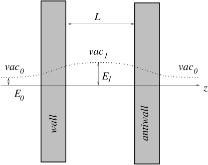
Figure 1: The wall-antiwall configuration in pure Yang–Mills theory at large $N$. The notation is as follows: $vac_{0}$ stands for the lowest-energy state, while $vac_{1}$ is the adjacent quasivacuum. The corresponding energy densities are $E_{0}$ and $E_{1}$, respectively. The wall-antiwall pair experiences linear confinement with the energy of the wall-antiwall pair configuration growing as $(E_{1}-E_{0})L$.

Now, this picture drastically changes once the axion field is added. In Ref. [10] (see also [11]) it was shown that the domain walls of pure Yang–Mills theory develop an axion component, axion tails with thickness $\sim m_{a}^{-1}$ where $m_{a}$ is the axion mass.

What is most important, the presence of the axion tails equalizes the vacuum energies on both sides of the wall. This is due to the fact that one can view the axion field on the wall as an interpolation between $\theta=0$ and $\theta=2\pi$. As $\theta_{\rm eff}$ adiabatically changes, the vacua “breathe” and effectively interchange their energies in the course of interpolation. $E_{1}$ becomes equal to $E_{0}$.

This means that the walls become absolutely stable, even at finite and not necessarily large $N$. Each wall can be considered in isolation. If we still consider the wall-antiwall configuration with separation $\gg m_{a}^{-1}$, as in Fig. 1, there is no force between the wall and antiwall. In other words, the wall confinement is gone at distances $\gg m_{a}^{-1}$.

In the $CP(N-1)$ model the role of walls is assumed by kinks. It was noted long ago [1] that at large $N$ the $CP(N-1)$ model is solvable within the framework of $1/N$ expansion, and this solution exhibits the following features: (i) a kink mass term of order $\Lambda$ develops which does not scale with $N$ (here $\Lambda$ is a dynamical scale parameter); (ii) isolated kinks do not exist in the physical spectrum; the physical spectrum is saturated by kink-antikink bound states; (iii) there is a linear potential acting between kinks and antikinks; the slope of this potential is small at large $N$ since it scales as $\Lambda^{2}/N$.

A close analogy with the domain wall confinement in four dimensions is evident. The root of this analogy is similarity of the vacuum structure. Much in the same way as in pure Yang–Mills theory in four dimension, the two-dimensional $CP(N-1)$ model has $\sim N$ quasivacua which become stable and degenerate at $N=\infty$. These vacua are all entangled in the $\theta$ evolution.

Below we will show that this analogy extends even further. Namely, if the axion field is introduced in the $CP(N-1)$ model, the kink-antikink confinement is eliminated. The force between them vanishes for separations $\gg m_{a}^{-1}$. The exact solvability of the $CP(N-1)$ model allows us to describe this phenomenon in fully quantitative terms using the framework developed in [1].

In the second part of this paper we return to the four-dimensional bulk theory supporting non-Abelian strings. In [3] it was shown that the $\theta$ term of this theory penetrates in the $CP(N-1)$ model on the world-sheet of the non-Abelian string. Recently non-Abelian strings were suggested as candidates for cosmic strings [13]. Then it is natural to promote the bulk $\theta$ term to a four-dimensional axion field and discuss its impact on the non-Abelian strings. In particular, we will be mostly interested in the fate of the kink-antikink pairs in the presence of the four-dimensional axion. In fact, the kinks can be identified with confined monopoles residing on the non-Abelian flux tubes [14, 6]. It turns out that the four-dimensional axion, unlike its two-dimensional counterpart, does not affect confinement of the monopole-antimonopole pairs on the cosmic string. The main effect due to four-dimensional axions is that excitation of these pairs results in the axion radiation. We will briefly comment on the emission of the “cosmic” axions off the non-Abelian strings.

The paper is organized as follows. In Sect. 2 we consider two-dimensional axion in the two-dimensional $CP(N-1)$ model and show that the axion-induced deconfinement of kinks takes place. Section 3 is devoted to four-dimensional axion interaction with non-Abelian flux tubes. Orientational moduli of such strings are described by the $CP(N-1)$ model on the string world-sheet. After a brief outline of the basic bulk model (Sect. 3.1) we introduce a bulk axion and argue that the four-dimensional axion does not liberate monopole-antimonopole pairs attached to the string and confined inside “mesons” (Sect. 3.2). Section 3.3 treats the axion radiation in the bulk in the context of non-Abelian cosmic strings.

2 Axion induced deconfinement of kinks in two dimensions

For our purposes the most convenient formulation of the $CP(N-1)$ model is in terms of the $n$ fields. Then the $CP(N-1)$ model can be written as

$${\cal L}=\frac{2}{g^{2}}\,\left[\left(\partial_{\alpha}+iA_{\alpha}\right)n^{*}_{\ell}\left(\partial_{\alpha}-iA_{\alpha}\right)n^{\ell}-\lambda\left(n^{*}_{\ell}n^{\ell}-1\right)\right]\,,$$ (1)

where $n^{\ell}$ is an $N$-component complex filed, $\ell=1,2,...,N$, subject to the constraint

$$n_{\ell}^{*}\,n^{\ell}=1\,.$$ (2)

This constraint is implemented by the Lagrange multiplier $\lambda$ in Eq. (1). The field $A_{\alpha}$ in this Lagrangian is also auxiliary, it enters with no derivatives and can be eliminated by virtue of the equations of motion,

$$A_{\alpha}=-\frac{i}{2}\,n^{*}_{\ell}\stackrel{{\scriptstyle\leftrightarrow}}{{\partial_{\alpha}}}n^{\ell}\,.$$ (3)

Substituting Eq. (3) in the Lagrangian, we rewrite it in the form

$${\cal L}=\frac{2}{g^{2}}\,\left[\partial_{\alpha}n^{*}_{\ell}\,\partial_{\alpha}n^{\ell}+(n_{\ell}^{*}\partial_{\alpha}n^{\ell})^{2}-\lambda\left(n^{*}_{\ell}n^{\ell}-1\right)\right]\,.$$ (4)

Now, $g^{2}$ is the coupling constant. The factor of $2$ in the definition of the coupling constant (see Eq. (1)) is introduced to match the standard definition of the coupling constant in the O(3) sigma model. The coupling constant $g^{2}$ is asymptotically free, and defines a dynamical scale of the theory $\Lambda$ through

$$\Lambda^{2}=M_{\rm uv}^{2}\exp\left(-\frac{8\pi}{Ng^{2}_{0}}\right)\,,$$ (5)

where $M_{\rm uv}$ is the ultraviolet cut-off and $g^{2}_{0}$ is the bare coupling.

At first, let us forget for a while about the axion terms and outline the solution of the “axionless” $CP(N-1)$ model at large $N$ [1]. To the leading order it is determined by one loop and can be summarized as follows: the constraint (2) is dynamically eliminated so that all $N$ fields $n^{\ell}$ become independent degrees of freedom with the mass term $\Lambda$. The photon field $A_{\mu}$ acquires a kinetic term

$${\cal L}_{\gamma\,\,\rm kin}=-\frac{1}{4e^{2}}F_{\mu\nu}^{2}\,,\qquad e^{2}=\frac{12\pi\Lambda^{2}}{N}\,,$$ (6)

and also becomes “dynamical.” We use quotation marks here because in two dimensions the kinetic term (6) does not propagate any physical degrees of freedom; its effect reduces to an instantaneous Coulomb interaction. This is best seen in the $A_{1}=0$ gauge. In this gauge the above kinetic term takes the form

$$(\partial_{z}A_{0})^{2}$$ (7)

while the interaction is

$$A_{\alpha}J^{\alpha}=A_{0}J^{0}\,,\qquad J^{\alpha}=n^{*}_{\ell}\stackrel{{\scriptstyle\leftrightarrow}}{{\partial_{\alpha}}}n^{\ell}\,.$$ (8)

Since $A_{0}$ enters in the Lagrangian without time derivative, it can be eliminated by virtue of the equation of motion leading to the instantaneous Coulomb interaction

$$J_{0}\,\partial_{z}^{-2}\,J_{0}\,.$$ (9)

In two dimensions the Coulomb interaction is proportional to

$$\frac{\Lambda^{2}}{N}\,|z|\,.$$ (10)

We get linear confinement acting between the $n,\,\,\bar{n}$ “quarks.”

The axion part of the Lagrangian can be written as follows:

$${\cal L}_{a}=f_{a}^{2}\,(\partial_{\mu}a)^{2}+\frac{a}{2\pi}\,\varepsilon_{\alpha\gamma}\partial^{\alpha}A^{\gamma}\,,$$ (11)

where $A^{\gamma}$ is defined in Eq. (3), and $f_{a}$ is the axion constant. In two dimensions it is dimensionless. As usual, the axion mass will be proportional to $\Lambda/f_{a}$. We will consistently assume that $f_{a}\gg 1$.

Upon field rescaling bringing kinetic terms to canonical normalization one obtains

$$-\frac{1}{4}F^{2}_{\mu\nu}+\frac{e}{2\pi f_{a}}\,a\,\varepsilon_{\alpha\gamma}\partial^{\alpha}A^{\gamma}+(\partial_{\mu}a)^{2}+e\,A_{\alpha}J^{\alpha}\,.$$ (12)

The axion field represents a single degree of freedom. The role of the “photon” is that upon diagonalization we get a massive spin-zero particle, with mass of order $f_{a}^{-1}\Lambda N^{-1/2}$.

Since the exchanged quanta are massive the long distance force responsible for confinement disappears, giving place to deconfinement at distances $\gg m_{a}^{-1}$.

Figure 2: The photon-axion mixing. Wavy lines denote photons, solid thin lines axions. Closed circles stand for the photon axion coupling $e/(2\pi f_{a})$ where $e$ is defined in Eq. (6). The photon are coupled to to the currents (thick solid lines) with the coupling constant $e$.

Taking account of the photon-axion mixing amounts to summing the infinite series of graphs depicted in Fig. 2. Using Eqs. (9) and (12) it is not difficult to get for this sum

$$e^{2}J^{0}J^{0}\left\{\frac{1}{p^{2}}+\frac{1}{p^{2}}\left(\frac{e}{2\pi f_{a}}\right)^{2}\,\frac{1}{p_{\mu}^{2}}+...\right\}=\frac{e^{2}J^{0}J^{0}}{p^{2}}\,\,\frac{p_{\mu}^{2}}{p_{\mu}^{2}-\left(\frac{e}{2\pi f_{a}}\right)^{2}}\,.$$ (13)

where $p$ is the spatial component of the momentum transfer $p_{\mu}$. Using the current conservation one can rewrite

$$J^{0}J^{0}\,p_{\mu}^{2}=-p^{2}\,J_{\alpha}J^{\alpha}\,,$$ (14)

which leads to the following final result for the sum of the graphs depicted in Fig. 2:

$$-e^{2}J_{\alpha}J^{\alpha}\,\,\frac{1}{p_{\mu}^{2}-\left(\frac{e}{2\pi f_{a}}\right)^{2}}\,.$$ (15)

This expression is Lorentz invariant; it describes propagation of a quantum of mass $e/(2\pi f_{a})$. At distances larger than $2\pi f_{a}/e$ the force acting between $n$ and $\bar{n}$ is exponentially screened. If instead of the emitter of “photons” we consider an emitter of axions and sum up the series of diagrams similar to that in Fig. 2 we arrive at the same pole as in Eq. (15). Of course, this is fully consistent with the fact that the photon-axion system in the problem at hand presents only one physical degree of freedom.

Note that the situation is very similar to the supersymmetric $CP(N-1)$ model whose physical spectrum consists of the kinks in the fundamental representation that are not confined [1]. The reason for the kink liberation in this case is as follows. The supersymmetric model involves massless fermions which interact with the photon field as $\bar{\psi}\gamma_{\mu}A_{\mu}\psi$. The massless fermions can be bosonized into the massless $\phi$ scalar with the interaction term $\epsilon^{\mu\nu}A_{\mu}\partial_{\nu}\phi$, which is the same as the photon-axion interaction in Eq. (12).

The axion-induced liberation of kinks at distances $\gg m_{a}^{-1}$ we have just demonstrated is the two-dimensional counterpart of domain-wall deconfinement in four-dimensions [10, 11]. The parallel becomes even more pronounced in the (string-inspired) formalism which ascends to [15] (in connection with walls it was developed in [10] and recently discussed in [16] in another context). In this formalism one introduces an (auxiliary) antisymmetric three-form gauge field $C_{\alpha\beta\gamma}$, while the four-dimensional axion is replaced by an antisymmetric two-form field $B_{\mu\nu}$ (the Kalb–Ramond field). In four dimensions the gauge three-form field has no propagating degrees of freedom while the Kalb–Ramond field $B_{\mu\nu}$ presents a single degree of freedom. The domain walls are the sources for $C_{\alpha\beta\gamma}$, much in the same way as the kinks are the sources for $A_{0}$ in two dimensions. The field strength four-form built from $C_{\alpha\beta\gamma}$ is constant (cf. $F_{01}$ in two dimensions). The $CB$ mixing produces one massive physical degree of freedom, four-dimensional massive axion. Simultaneously, the domain-wall confinement is eliminated at distances $\gg m_{a}^{-1}$. In full analogy with two-dimensional $CP(N-1)$, supersymmetrization of Yang–Mills theory leads to wall deconfinement without axion’s help.

Can one understand this phenomenon in the language we used in Sect. 1 for description of the wall confinement/deconfinement? The answer is yes, the underlying physics is basically the same. In the “axionless” $CP(N-1)$ model there are $\sim N$ quasivacua split in energy, the splitting being of order of $\Lambda^{2}/N$ (labeled by an integer $k$). Only the lower minimum is the true vacuum while all others are metastable exited states. [In the large $N$ limit the decay rate is exponentially small, $\sim\exp(-N)$.] At large $N$, the $k$ dependence of the energy density on the quasivacua, as well as the $\theta$ dependence, is well-known

$${E}_{k}(\theta)\sim\,N\,\Lambda^{2}\left\{1+{\rm const}\,\left(\frac{2\pi k+\theta}{N}\right)^{2}\right\}\,.$$ (16)

At $\theta=0$ the genuine vacuum corresponds to $k=0$, while the first excitation to $k=-1$. At $\theta=\pi$ these two vacua are degenerate, at $\theta=2\pi$ their roles interchange.

The energy split ensures kink confinement: kinks do not exist as asymptotic states — instead, they form kink-antikink mesons. The regions to the left of the kink and to the right of the antikink are the domains of the true vacuum (at $\theta=0$ it corresponds to $k=0$.) The region between the kink and antikink is an insertion of the adjacent quasivacuum with $k=-1$.

When we introduce the axion, the vacuum angle $\theta$ is replaced by a dynamical field, $a(t,z)$. In the regions to the left of the kink and to the right of the antikink $\langle a\rangle=0$. If the region between the kink and antikink is large enough, $L\gg m_{a}^{-1}$, the axion field in this region adjusts itself in such a way as to minimize energy,

$$\langle a\rangle=0\longrightarrow\langle a\rangle=2\pi\,.$$

This axion tail equalizes the energy densities to the left and to the right of the kink (as well as to the left and to the right of the antikink) liberating $n$ and $\bar{n}$ from confinement.

3 Four-dimensional axion and non-Abelian
strings

In Sect. 2 we showed that introducing two-dimensional axion in (nonsupersymmetric) $CP(N-1)$ liberates kinks. Now, let us address another aspect. Let us introduce a four-dimensional axion in the bulk theory which supports non-Abelian strings and confined monopoles seen as kinks in the world-sheet theory (also $CP(N-1)$). Then we study the impact of this four-dimensional axion on dynamics of strings/confined monopoles.

3.1 The bulk model with non-Abelian strings

First, let us briefly outline the model. Following [3] we consider a nonsupersymmetric model which is in fact a bosonic truncation of ${\cal N}=2$ model. It supports non-Abelian strings. The key requirement is the existence of color-flavor locking which provides topological stability to the stringy solutions of first-order equations analogous to BPS equations of the supersymmetric “parent.” The action has the form [3] (in the Euclidean notation)

$$S = \int{\rm d}^{4}x\left\{\frac{1}{4g_{2}^{2}}\left(F^{a}_{\mu\nu}\right)^{2}+\frac{1}{4g_{1}^{2}}\left(F_{\mu\nu}\right)^{2}\right.$$ (17)

$$+ {\rm Tr}\,(\nabla_{\mu}\Phi)^{\dagger}\,(\nabla^{\mu}\Phi)+\frac{g^{2}_{2}}{2}\left[{\rm Tr}\,\left(\Phi^{\dagger}T^{a}\Phi\right)\right]^{2}+\frac{g^{2}_{1}}{8}\left[{\rm Tr}\,\left(\Phi^{\dagger}\Phi\right)-N\xi\right]^{2}$$

$$+ \left.\frac{i\,\theta}{32\,\pi^{2}}\,F_{\mu\nu}^{a}\tilde{F}^{a\,\mu\nu}\right\}\,,$$

where $T^{a}$ stands for the generator of the gauge SU($N$),

$$\nabla_{\mu}\,\Phi\equiv\left(\partial_{\mu}-\frac{i}{\sqrt{2N}}\;A_{\mu}-iA^{a}_{\mu}\,T^{a}\right)\Phi\,,$$ (18)

and $\theta$ is the vacuum angle, to be promoted to the axion field,

$$\theta\to\theta+a\to a(x)\,.$$ (19)

The last term forces $\Phi$ to develop a vacuum expectation value (VEV) while the last but one term forces the VEV to be diagonal,

$$\Phi_{\rm vac}=\sqrt{\xi}\,{\rm diag}\,\{1,1,...,1\}\,.$$ (20)

This VEV results in the spontaneous breaking of both gauge and flavor SU($N$)’s. A diagonal global SU($N$) survives, however, namely

$${\rm U}(N)_{\rm gauge}\times{\rm SU}(N)_{\rm flavor}\to{\rm SU}(N)_{\rm diag}\,.$$ (21)

Thus, color-flavor locking takes place in the vacuum.

One can combine the $Z_{N}$ center of SU($N$) with the elements $\exp(2\pi ik/N)\in$U(1) to get a topologically stable string solution [4, 5] possessing both windings, in SU($N$) and U(1) since

$$\pi_{1}\left({\rm SU}(N)\times{\rm U}(1)/Z_{N}\right)\neq 0\,.$$ (22)

Their tension is $1/N$-th of that of the ANO string hence the ANO string can be considered as a bound state of $N$ elementary strings. These elementary strings are $Z_{N}$ strings.

The most important feature of $Z_{N}$ strings in the model (17) is that they acquire orientational zero modes associated with rotation of their color flux inside the non-Abelian subgroup SU($N$) of the gauge group [4, 5, 6, 7]. This makes these strings genuinely non-Abelian. This means that the effective low-energy theory on the string world-sheet includes both the standard Nambu-Goto action associated with translational moduli and a sigma model which describes internal dynamics of the orientational moduli.

As was mentioned above, the emerging world-sheet action can be identified as the $CP(N-1)$ sigma model [4, 5, 6, 7] which (in the Euclidean notation) is given by the action

$$S^{(1+1)}=\int dt\,dz\,\left\{2\beta\,\left[(\partial^{k}\,n^{*}\partial_{k}\,n)+(n^{*}\partial_{k}\,n)^{2}\right]-\frac{\theta+a}{2\pi}\,\,\varepsilon^{nk}\,\partial_{n}\,n^{*}\partial_{k}\,n\right\}\,,$$ (23)

where $\theta$ coincides with the four-dimensional $\theta$ while

$$\beta=\frac{2\pi}{g^{2}_{2}}.$$ (24)

The bulk theory is fully Higgsed, hence, the monopoles are in the confinement phase. In fact, as it was shown in [14, 6, 3], they manifest themselves as junctions of distinct elementary non-Abelian strings. In the string world-sheet theory (23) they are seen as kinks $n$ and $\bar{n}$ interpolating between the true vacuum and the adjacent quasivacuum of the $CP(N-1)$ model (each quasivacuum in the $CP(N-1)$ model corresponds to a particular elementary string).

From the four-dimensional point of view this means that, besides four-dimensional confinement, the monopoles are confined also in the two-dimensional sense: if a monopole is attached to a string, with necessity there is an antimonopole attached to the same string, and they form a meson-like configuration on the string [17, 3], see Fig. 3.

Figure 3: Monopole-antimonopole meson attached to the string. The filled circle denotes the monopole while the empty circle antimonopole. The thick line between the monopole and antimonopole denotes the region of an exited string with $k=-1$.

3.2 Monopole-antimonopole “mesons” vs. axion clouds

In this section we address the question what happens with the monopole-antimonopole meson on the non-Abelian string in the presence of the four-dimensional axion. A priori one might suspect that the four-dimensional axion induces deconfinement of monopoles localized on the non-Abelian string, much in the same way as the two-dimensional axion. Below we show that this does not happen.

The classical action of the four dimensional bulk axion field is

$$L_{a}=\int d^{4}x\left[f_{a}^{2}(\partial a)^{2}+\frac{ia}{32\pi^{2}}F^{a}_{\mu\nu}\tilde{F}^{a}_{\mu\nu}\right]\,,$$ (25)

where in the case at hand $f_{a}$ has dimension of mass. The axion has a small mass generated by four-dimensional bulk instantons

$$m_{a}^{2}\sim\frac{\Lambda^{4}_{4}}{f_{a}^{2}}\,\left(\frac{\Lambda_{4}}{\sqrt{\xi}}\right)^{b-4},$$ (26)

where $b$ is the first coefficient of the $\beta$ function in the theory (17). As usual, it is assumed that $f_{a}\gg\Lambda_{4}$.

The impact of the bulk axion on non-Abelian string is two-fold. First, the axion gets coupled to the translational moduli of the string. Assuming that the string collective coordinates adiabatically depend on the world-sheet coordinates we get for this coupling

$${\cal L}_{a}^{(1)}\sim\xi\int d^{4}x\,a(x)\,\varepsilon^{ij}\,\varepsilon_{\alpha\beta}\,\partial_{i}x^{\alpha}\,\partial_{j}x^{\beta}\,\,\delta^{(2)}(x-x_{\rm string}(t,z)),$$ (27)

where the indices $i,j=0,3$ run over the string world sheet coordinates while the indices $\alpha,\beta=1,2$ are orthogonal to the string world-sheet. One could rewrite this expression in the covariant form trading the axion field for the Kalb-Ramon two-index field $B_{\mu\nu}(x)$. However, for our purposes this is not necessary. The coupling (27) is not specific for non-Abelian strings, it is generated in the case of the Abelian (or $Z_{N}$) strings as well.

Now, let us discuss compact orientational moduli. It is easy to see that no mixed $n$-$x$ terms appear in the axion Lagrangian (at least, in the the quadratic order in derivatives). The bulk axion generates a quadratic in $n$ coupling, as is clearly seen from Eq. (23). The impact of this term in the axion Lagrangian can be summarized as follows:

$${\cal L}_{a}^{(2)}\sim\int d^{4}x\,a(x)\,\varepsilon^{nk}\,\,\partial_{n}\,n^{*}\partial_{k}\,n\,\,\delta^{(2)}(x-x_{\rm string}(t,z)),$$ (28)

Consider the monopole-antimonopole pair attached to the string, as in Fig. 3, where the axion is switched off. For $k=0$ the string is in the state with the lowest energy. The monopole-antimonopole meson on the string corresponds to the region of the excited $k=-1$ string between the monopole and antimonopole while to the left of the monopole and to the right of the antimonopole $k=0$. The energy of this meson is of order of $(\Lambda^{2}/N)\,L,$ where $L$ is the distance between the monopole and antimonopole along the string.

Now, let us switch on the four-dimensional axion field. What could happen (but, in fact, does not happen) is that the axion field could develop a non-vanishing expectation value $a=2\pi$ on the string between the monopole and antimonopole positions, equalizing the string energies and thus screening the confinement force. This is exactly what happened for the two-dimensional axion studied in Sect. 2.

To see whether or not a similar effect occurs with four-dimensional axion we have to examine a field configuration in which $\langle a\rangle=0$ everywhere in the bulk except a region adjacent to the monopole-antimonopole separation interval, as depicted in Fig. 4. We have to check the energy balance assuming there is an axion cloud such that on the string inside the monopole-antimonopole separation interval $\langle a\rangle=2\pi$, which would let (anti)monopoles attached to the string move freely along the string, with no confinement along the string.

It is not difficult to estimate the energy of the axion cloud. Transverse size of the cloud (in two directions perpendicular to the string) must be of order of $m_{a}^{-1}$. The longitudinal dimension is $L$, see Fig. 4. Assume that $L\gg m_{a}^{-1}$. Then we get

$$E_{\rm cloud}\sim f_{a}^{2}\,L,$$ (29)

to be compared to the energy $(\Lambda^{2}/N)\,L$ of the monopole-antimonopole meson.

Figure 4: The monopole-antimonopole meson together with the axion cloud. The region of the string between the monopole and antimonopole is not exited because although this region has $k=-1$ the value of the axion field is non-zero inside the axion cloud, $a=2\pi$.

Since $f_{a}$ is supposed to be very large compared to $\Lambda$ we see that the energy of the axion cloud (29) is much larger than the energy of monopole-antimonopole meson. Developing a compensating axion cloud is energetically disfavored. Therefore we conclude that there is no monopole deconfinement driven by four-dimensional axion.

Another way to arrive at the same conclusion involves consideration of the propagator of the four-dimensional axion between two points on the string world-sheet, along the lines of Ref. [18]. Analysis we performed in the momentum space shows that there is no macroscopic region with the two-dimensional behavior on this propagator.

3.3 Cosmic non-Abelian string and axion emission

Recently it was suggested [13] to consider non-Abelian strings as cosmic string candidates. Therefore it is worth discussing possible signatures of such non-Abelian strings. Obviously, they can be excited in collisions. Both, translational and orientational modes can be excited. In the latter case one can think of production of energetic monopole-antimonopole pairs attached to the string and bound in mesons by the confining potential along the string, as described in Sect. 3.2. In Ref. [13] it was suggested that isolated monopoles (kinks) can be created on cosmic strings nonperturbatively. It is obvious that in our non-supersymmetric case only pair creation is allowed. Let us return to Fig. 3. On the part of the string between the monopole and antimonopole (the kink and antikink) the state of the string is described by the quasivacuum with $k=-1$. In this state 

$$\langle\varepsilon^{nk}\,\,\partial_{n}\,n^{*}\partial_{k}\,n\rangle\sim\Lambda^{2}/N\,.$$ (30)

The topological charge density is localized in the domain of the excited part of the string, and is approximately constant in this domain. Therefore, as is clear from Eq. (28), this interval, whose length $L$ oscillates in accordance with the monopole-antimonopole motion, will serve as a source term in the equation for the axion field. Assume that the energy of the kink-antikink pair $E\gg\Lambda$ so that they can be treated quasiclassically. The distance $L$ between the kink and antikink will oscillate between $-L_{0}$ and $L_{0}$ where $L_{0}\sim E/\Lambda^{2}$ with the frequency $\omega\sim\Lambda^{2}/E$,

$$L(t)=L_{0}\,e^{i\omega t}\,.$$ (31)

Therefore, for a distant observer the monopole-antimonopole meson is seen as a point-like source with the interaction term

$${\Lambda^{2}}\,\int d^{4}x\,a(x)\,L(t)\,\delta^{3}(r-r_{0}),$$ (32)

where $r_{0}$ is a position of the meson on the string. The intensity of the axion radiation from this point-like source can be estimated as

$$I_{a}\sim\omega^{2}\,\frac{\Lambda^{4}L^{2}_{0}}{f_{a}^{2}}\,\frac{1}{r^{2}}\sim\omega^{2}\,\frac{E^{2}}{f_{a}^{2}}\,\frac{1}{r^{2}}\,,$$ (33)

where $r$ is the distance to the observer.

Of course the string produces axion radiation also due to coupling with translational modes, Eq. (27). This radiation is seen as coming from a linear source, and can be estimated (per unit length) as

$$I_{a}\sim\frac{\xi^{1/2}}{f_{a}^{2}}\,\frac{E^{2}}{\ell^{2}}\,\frac{1}{\rho}\,.$$ (34)

Here $\rho$ is the distance from the string to the observer in the plane orthogonal to the string, $E$ is the total excitation energy and $\ell$ is the length of the excited part of the string. This radiation is not specific for non-Abelian strings. Abelian ($Z_{N}$) strings produce this radiation as well.

Thus we see that the non-Abelian string is seen by a distant observer as a linear source of the axion radiation (34), with additional point-like sources of the axion radiation (33) located on the linear source at the positions of the monopole-antimonopole mesons.

The rate of the axion radiation depends of $f_{a}$. The oscillating kink-antikink pair will shake off energy until annihilation. The time duration of the monopole-antimonopole meson de-excitation can be estimated as $T\sim E^{2}f_{a}^{2}$.

4 Conclusion

The existence of the axion is almost unavoidable in the framework of string theory. In this paper we discussed how axions affect dynamics of strongly interacting objects. The first part of the paper is devoted to a toy two-dimensional model, nonsupersymmetric $CP(N-1)$, in which axions produce a dramatic effect: they liberate kinks (confined in the absence of axion) at distances $\gg m_{a}^{-1}$. Thus, we observed a novel phenomenon of axion-induced deconfinement of kinks.

This phenomenon is akin to the domain wall liberation by axions in four-dimensional (nonsupersymmetric) Yang–Mills theory [10, 11].

Proceeding to four dimensions, we introduced a bulk axion in the “benchmark” nonsupersymmetric model [3] supporting non-Abelian strings. Unlike its two-dimensional counterpart, the four-dimensional axion does not lead to monopole deconfinement.

Considering non-Abelian strings in the context of cosmic strings we discussed axion emission due to excitations of such strings. The excitations which produce axion radiation are of two types: (i) excitations of the translational modes (the shape of the string), and (ii) production of energetic pairs of confined (anti)monopoles. The latter is specific to the non-Abelian strings. We estimated the intensity of the axion radiation off the string and the time duration of the de-excitation process.

References

- [1] E. Witten, Nucl. Phys. B 149, 285 (1979).
- [2] V. A. Novikov, M. A. Shifman, A. I. Vainshtein and V. I. Zakharov, Phys. Rept. 116, 103 (1984).
- [3] A. Gorsky, M. Shifman and A. Yung, Phys. Rev. D 71, 045010 (2005) [hep-th/0412082].
- [4] A. Hanany and D. Tong, JHEP 0307, 037 (2003) [hep-th/0306150].
- [5] R. Auzzi, S. Bolognesi, J. Evslin, K. Konishi and A. Yung, Nucl. Phys. B 673, 187 (2003) [hep-th/0307287].
- [6] M. Shifman and A. Yung, Phys. Rev. D 70, 045004 (2004) [hep-th/0403149].
- [7] A. Hanany and D. Tong, JHEP 0404, 066 (2004) [hep-th/0403158].
- [8] E. Witten, Phys. Rev. Lett. 81, 2862 (1998) [hep-th/9807109].
- [9] M. Shifman, Phys. Rev. D 59, 021501 (1999) [hep-th/9809184].
- [10] G. Gabadadze and M. A. Shifman, Phys. Rev. D 62, 114003 (2000) [hep-ph/0007345].
- [11] G. Gabadadze and M. Shifman, Int. J. Mod. Phys. A 17, 3689 (2002) [hep-ph/0206123].
- [12] H. B. Thacker, D-branes and topological charge in QCD, hep-lat/0509057; S. Ahmad, J. T. Lenaghan and H. B. Thacker, Phys. Rev. D 72, 114511 (2005) [hep-lat/0509066].
- [13] K. Hashimoto and D. Tong, JCAP 0509, 004 (2005) [hep-th/0506022].
- [14] D. Tong, Phys. Rev. D 69, 065003 (2004) [hep-th/0307302].
- [15] R. Kallosh, A. D. Linde, D. A. Linde and L. Susskind, Phys. Rev. D 52, 912 (1995) [hep-th/9502069].
- [16] G. Dvali, Three-Form Gauging of Axion Symmetries and Gravity, hep-th/0507215.
- [17] V. Markov, A. Marshakov and A. Yung, Nucl. Phys. B 709, 267 (2005) [hep-th/0408235].
- [18] G. R. Dvali, G. Gabadadze and M. Porrati, Phys. Lett. B 485, 208 (2000) [hep-th/0005016].