hep-th/0601126

Graviton Emission in the Bulk from a
Higher-Dimensional Schwarzschild Black Hole

S. Creek¹, O. Efthimiou², P. Kanti¹ and K. Tamvakis²

¹ Department of Mathematical Sciences, University of Durham,
Science Site, South Road, Durham DH1 3LE, United Kingdom

² Division of Theoretical Physics, Department of Physics,
University of Ioannina, Ioannina GR-45110, Greece

Abstract

We consider the evaporation of $(4+n)$-dimensional non-rotating black holes into gravitons. We calculate the energy emission rate for gravitons in the bulk obtaining analytical solutions of the master equation satisfied by all three types (S,V,T) of gravitational perturbations. Our results, valid in the low-energy regime, show a vector radiation dominance for every value of $n$, while the relative magnitude of the energy emission rate of the subdominant scalar and tensor radiation depends on $n$. The low-energy emission rate in the bulk for gravitons is well below that for a scalar field, due to the absence of the dominant $\ell=0,1$ modes from the gravitational spectrum. Higher partial waves though may modify this behaviour at higher energies. The calculated low-energy emission rate, for all types of degrees of freedom decreases with $n$, although the full energy emission rate, integrated over all frequencies, is expected to increase with $n$, as in the previously studied case of a bulk scalar field.

1 Introduction

The quest for unification of fundamental interactions with gravity has led to the idea of extra spatial dimensions. String Theory, or some form of it, considered at present as a promising consistent theoretical framework for such a unification at the quantum level, requires extra spatial dimensions. In this higher-dimensional context, which has received a lot of attention in the last few years [1, 2], gravity propagates in $D=4+n$ dimensions (Bulk), while all Standard Model degrees of freedom are assumed to be confined on a four-dimensional $D$-Brane. In theories with large extra dimensions [1] the traditional Planck scale $M_{Pl}\sim 10^{18}$ GeV is only an effective scale, related to the fundamental higher-dimensional gravity scale $M_{*}$ through the relation $M_{Pl}^{2}\sim M_{*}^{n+2}R^{n}$, where $R\sim(V_{n})^{1/n}$ is the effective size of the $n$ extra spatial dimensions. If $R\gg\ell_{Pl}\approx 10^{-33}\,cm$, the scale $M_{*}$ can be substantially lower than $M_{Pl}$. If $M_{*}$ is sufficiently low, trans-planckian particle collisions could be feasible in accelerators or other environments. The product of such collisions would be objects that probe the extra dimensions. Black holes are among the possible products of trans-planckian collisions [3]. Black holes with a horizon size $r_{H}$ smaller than the size of extra dimensions $R$ will be higher-dimensional objects centered at the brane and extending in the bulk. A classical treatment would require that the mass of the black hole $M_{BH}$ would have to be larger than the fundamental gravity scale $M_{*}$. Such black holes can be created in ground based colliders, although their appearance in cosmic rays is possible as well (for references, see the reviews [4, 5]). A black hole created in such trans-planckian collisions is expected to undergo a short “balding” phase in which it will shed its additional quantum numbers, apart from charge, angular momentum and mass. Then, after a more familiar Kerr-like phase, in which it will lose its angular momentum, a Schwarzschild phase follows during which the black hole will gradually lose its mass through the emission of Hawking radiation both in the bulk and in the brane, consisting of elementary particles of a very distinct thermal spectrum. This black hole radiation has been the subject of both analytical and numerical studies. This includes lower spin degrees of freedom [7, 8, 9, 10, 11, 12] as well as graviton emission in the bulk [13]. The study of graviton emission in the bulk corresponds to the study of perturbations in a gravitational background. The formalism for the treatment of gravitational perturbations of a higher-dimensional non-rotating black hole has been developed in [14]. In the present article we consider the evaporation of $(4+n)$-dimensional non-rotating black holes into gravitons and calculate the energy emission rate for gravitons in the bulk obtaining analytical solutions of the master equation satisfied by gravitational perturbations. Our results, valid in the low-energy regime, are complementary to existing studies in the intermediate energy regime [13]. These results show a vector radiation dominance for every value of $n$, while the relative magnitude of the energy emission rate of the subdominant scalar and tensor radiation depends on $n$. The low-energy emission rate in the bulk for gravitons is well below that for a scalar field, due to the absence of the dominant $\ell=0,1$ modes from the gravitational spectrum, although higher partial waves are likely to modify this behaviour at higher energies. The calculated low-energy emission rate, for all types of degrees of freedom decreases with $n$, although the full energy emission rate, integrated over all frequencies, is expected to increase with $n$, as in the previously studied case of a bulk scalar field.

2 Theoretical Framework

According to the Large Extra Dimensions scenario [1], our universe is made up of the usual 3+1 non-compact dimensions plus $n$ additional, compact, spacelike ones. The gravitational background around a spherically-symmetric, neutral black hole formed in such a $(4+n)$-dimensional, flat spacetime is described by the following line-element [15]

$$ds^{2}=-f(r)\,dt^{2}+\frac{dr^{2}}{f(r)}+r^{2}d\Omega_{2+n}^{2},$$ (1)

with the metric function $f(r)$ given by

$$f(r)=1-\left(\frac{r_{H}}{r}\right)^{n+1}\,,$$ (2)

and $d\Omega_{2+n}^{2}$ denoting the area of the ($2+n$)-dimensional unit sphere. The above black hole is characterized by a non-vanishing temperature given by

$$T_{H}=\frac{n+1}{4\pi r_{H}}\,,$$ (3)

and therefore emits Hawking radiation [6] with an energy emission rate that resembles the one for a black body. The strong gravitational field surrounding the black hole modifies the spectrum through the modification of the corresponding absorption probability $|{\cal A}|^{2}$, that now depends on the energy $\omega$ and spin $s$ of the emitted particle as well as on the number of extra dimensions $n$ (see, for example, [4]). The absorption probability can be found by solving the equation of motion of a particular field propagating in the vicinity of the black hole and by using classical scattering theory. As mentioned in the Introduction, in this work, we focus on the decay of a $(4+n)$-dimensional, Schwarzschild black hole through the emission of gravitons in the bulk.

Following [14], a graviton in $D$ dimensions can be decomposed into a symmetric traceless tensor, a vector and a scalar part. These are further expanded in terms of the spin-weighted spherical harmonics on the $S^{n+2}$ unit sphere. The radial parts of all three types of gravitational perturbations are found to satisfy a Schrodinger-like equation of the form [14]

$$f\frac{d}{dr}\left(f\,\frac{d\Phi}{dr}\right)+(\omega^{2}-V)\,\Phi=0\,.$$ (4)

The potential $V$ has a different form for each type of perturbation, namely

$$V_{T,V}=\frac{f(r)}{r^{2}}\,\left[l(l+n+1)+\frac{n(n+2)}{4}-\frac{k(n+2)^{2}}{4}\left(\frac{r_{H}}{r}\right)^{n+1}\right]\,,$$ (5)

for tensor- and vector-like perturbations, with $k=-1$ and $k=3$ respectively, and

$$V_{S}=\frac{f(r)}{r^{2}}\,\frac{qx^{3}+px^{2}+wx+z}{4\left[2m+(n+2)(n+3)x\right]^{2}}\,,$$ (6)

for scalar gravitational perturbations, with

$$m\equiv l(l+n+1)-n-2\,,\qquad x\equiv\left(\frac{r_{H}}{r}\right)^{n+1}=1-f\,,$$ (7)

and

$$q \equiv (n+2)^{4}(n+3)^{2}\,,\qquad z\,\,\,\equiv\,\,\,16m^{3}+4m^{2}(n+2)(n+4)\,,$$

$$p \equiv (n+2)(n+3)\left[4m\,(2n^{2}+5n+6)+n(n+2)(n+3)(n-2)\right],$$ (8)

$$w \equiv -12m\,(n+2)\,\left[m(n-2)+n(n+2)(n+3)\right].$$

3 Solving the Field Equations

In this section, we proceed to solve analytically the above equation for all three types of gravitational perturbations in the vicinity of a $(4+n)$-dimensional neutral, spherically-symmetric black-hole. For this purpose, we will use a well-known approximate method and solve first the aforementioned equation at the two asymptotic radial regimes: close to the black hole horizon ($r\simeq r_{H}$), and far away from it ($r\gg r_{H}$). The two solutions will then be stretched and matched in an intermediate zone to create a smooth analytical solution extending over the whole radial regime.

3.1 The Near-Horizon Regime

Here, we focus on the derivation of the solution for all types of gravitational perturbations in the asymptotic regime close to the black hole horizon. Due to the similar form of their potential, tensor and vector perturbations will be treated together, while the scalar perturbations will be dealt with separately.

A. Tensor and Vector Perturbations

We start by making the change of variable $r\rightarrow f(r)$, in terms of which the field equation for tensor and vector perturbations can be written in the form

$$f\,(1-f)\,\frac{d^{2}\Phi}{df^{2}}+\left[1-\frac{(2n+3)}{(n+1)}\,f\right]\frac{d\Phi}{df}+$$ (9)

$$\hskip 85.35826pt\biggl{[}\,\frac{(\omega r_{H})^{2}}{(n+1)^{2}f(1-f)}-\frac{A}{(1-f)}+\frac{k(n+2)^{2}}{4(n+1)^{2}}\,\biggr{]}\Phi=0\,.$$

In the above, $k=-1$ for tensor perturbations and $k=3$ for vector ones, and we have also defined for convenience the quantity

$$A\equiv\frac{l(l+n+1)}{(n+1)^{2}}+\frac{n(n+2)}{4(n+1)^{2}}\,.$$ (10)

If we now make the following field redefinition: $\Phi(f)=f^{\alpha}(1-f)^{\beta}F(f)$, the above equation takes the form of a hypergeometric equation

$$f\,(1-f)\,\frac{d^{2}F}{df^{2}}+[c-(1+a+b)\,f]\,\frac{dF}{df}-ab\,F=0\,,$$ (11)

under the identifications

$$a=\alpha+\beta+\frac{(n+2)}{2(n+1)}+G\,,\qquad b=\alpha+\beta+\frac{(n+2)}{2(n+1)}-G\,,\qquad c=1+2\alpha\,,$$ (12)

where $G$ an arbitrary constant. Demanding further that the coefficient of $F(f)$ in our equation be indeed $-ab$ yields three more additional constraints that determine the remaining unknown constants, $\alpha$, $\beta$ and $G$. Their corresponding values are found to be

$$G^{(T,\,V)}=\frac{(1+k)(n+2)}{4(n+1)}\,,\qquad\alpha_{\pm}=\pm\frac{i\omega r_{H}}{n+1}\,,$$ (13)

and

$$\beta=\frac{1}{2(n+1)}\,\left\{-1\pm\sqrt{(2l+n+1)^{2}-4\omega^{2}r_{H}^{2}}\right\}\,.$$ (14)

The indices of the hypergeometric equation $(a,b,c)$ are now fully determined, which allows us to write the general solution of the hypergeometric equation, and thus the solution in the near-horizon regime, as

$$\Phi_{NH}(f)=A_{1}f^{\alpha}\,(1-f)^{\beta}\,F(a,b,c;f)$$

$$\hskip 56.9055pt+\,A_{2}\,f^{-\alpha}\,(1-f)^{\beta}\,F(a-c+1,b-c+1,2-c;f)\,,$$ (15)

where $A_{1,2}$ are arbitrary integration constants. There is, however, a boundary condition that this general solution must satisfy: no outgoing waves must be found right outside the black-hole horizon, as nothing can escape from within this area. To ensure this, we expand our solution in the limit $r\rightarrow r_{H}$, or equivalently $f\rightarrow 0$, in which case we find

$$\Phi_{NH}(f)\simeq A_{1}\,f^{\alpha}+A_{2}\,f^{-\alpha}=A_{1}\,e^{-i\omega y}+A_{2}\,e^{i\omega y}\,,$$ (16)

where, in the last part of the above equation, we have used the ‘tortoise-like’ coordinate

$$\frac{dy}{dr}=\frac{r_{H}^{n+2}}{f(r)\,r^{n+2}}\,.$$ (17)

The asymptotic solution is therefore written in terms of incoming and outgoing plane waves, as expected, since very close to the horizon the potential $V$ for all types of gravitational perturbations vanishes. Nevertheless, the aforementioned boundary condition forces us to discard the outgoing wave by setting $A_{2}=0$, that brings the near-horizon solution to its final form

$$\Phi_{NH}(f)=A_{1}f^{\alpha}\,(1-f)^{\beta}\,F(a,b,c;f)\,.$$ (18)

The only task remaining is to fix the arbitrary signs appearing in the expressions of both $\alpha$ and $\beta$. As we may see from Eq. (16), the interchange $\alpha_{+}\leftrightarrow\alpha_{-}$ would simply interchange the integration coefficients $A_{1}\leftrightarrow A_{2}$, therefore the sign of $\alpha$ can be chosen at random; here, we have chosen $\alpha=\alpha_{-}$. On the other hand, the sign in $\beta$ can be fixed by the convergence condition of the hypergeometric function, i.e. ${\bf Re}\,(c-a-b)=-\frac{1}{n+1}-2\beta>0$, that clearly demands that we choose $\beta=\beta_{-}$.

B. Scalar Perturbations

By employing the same change of variable, the field equation for scalar gravitational perturbations can be brought to the form

$$f\,(1-f)\,\frac{d^{2}\Phi}{df^{2}}+\left[1-\frac{(2n+3)}{(n+1)}\,f\right]\frac{d\Phi}{df}+$$ (19)

$$\hskip 85.35826pt\biggl{[}\,\frac{(\omega r_{H})^{2}}{(n+1)^{2}f(1-f)}-\frac{z}{16(n+1)^{2}m^{2}(1-f)}-C\,\biggr{]}\Phi=0\,,$$

where we have defined the quantity

$$C\equiv\frac{q(1-f)^{2}+\tilde{p}(1-f)+\tilde{w}}{4(n+1)^{2}[2m+(n+2)(n+3)(1-f)]^{2}}\,,$$ (20)

with

$$\tilde{p}=p-\frac{z(n+2)^{2}(n+3)^{2}}{4m^{2}}\,,\qquad\tilde{w}=w-\frac{z(n+2)(n+3)}{m}\,.$$ (21)

In this form, Eq. (19) has poles at $f=0$ and $f=1$ (or, at $r=r_{H}$ and $r=\infty$, respectively) while the quantity $C$ takes on a constant value in both limits.

We then follow a similar method as before, and bring again Eq. (19) to the form of a hypergeometric equation, with the indices $(a,b,c)$ given by Eqs. (12), and the powers $(\alpha,\beta)$ by Eqs. (13)-(14). The only difference arises in the value of the arbitrary constant $G$ that, in the case of scalar perturbations, takes the value

$$G^{(S)}=\frac{1}{2(n+1)}\,\sqrt{(n+2)^{2}-\frac{q+\tilde{p}+\tilde{w}}{[2m+(n+2)(n+3)]^{2}}}\,.$$ (22)

By applying the same boundary condition of no-outgoing waves near the horizon, the general solution for scalar perturbations in the near-horizon regime is given again by Eq. (18), with $\beta=\beta_{-}$ and $\alpha=\alpha_{-}$, as before.

3.2 The Far-Field Regime

We now turn to the far-field regime. In the limit $r\gg r_{H}$, $f\rightarrow 1$, and the field equation for all types of gravitational perturbations – tensor, vector and scalar – takes the simplified form

$$\frac{d^{2}\Phi}{dr^{2}}+\left(\omega^{2}-\frac{(n+1)^{2}A}{r^{2}}\right)\Phi=0\,,$$ (23)

where $A$ was defined in Eq. (10). By further setting $\Phi=\sqrt{r}\,R$, the new radial function $R$ is found to satisfy a Bessel differential equation

$$\frac{d^{2}R}{dz^{2}}+\frac{1}{z}\,\frac{dR}{dz}+\left(1-\frac{\nu^{2}}{z^{2}}\right)R=0\,,$$ (24)

with $z=\omega r$ and $\nu=l+(n+1)/2$. Therefore, the general solution of Eq. (23), standing for the analytical solution in the far-field regime, can be written as

$$\Phi_{FF}(r)=B_{1}\sqrt{r}\,J_{l+(n+1)/2}\,(\omega r)+B_{2}\sqrt{r}\,Y_{l+(n+1)/2}\,(\omega r)\,,$$ (25)

where $J_{\nu}$ and $Y_{\nu}$ are the Bessel functions of the first and second kind, respectively, and $B_{1,2}$ arbitrary integration constants.

3.3 Constructing the complete solution

Having derived the two asymptotic analytical solutions near the black-hole horizon and infinity, we may now proceed to construct a solution valid at the whole radial regime by smoothly connecting the two solutions at an intermediate point. To this end, we need to stretch the near-horizon solution (18) towards large values of $r$, and the far-field solution (25) towards small values of $r$.

Before, however, being able to do the former, we need to rewrite the near-horizon solution in an alternative form where the argument of the hypergeometric function has been shifted from $f$ to $1-f$. To this end, we use the standard formula [16]

$$F(a,b,c;f) = \frac{\Gamma(c)\,\Gamma(c-a-b)}{\Gamma(c-a)\,\Gamma(c-b)}\,F(a,b,a+b-c+1;1-f)$$

$$+ (1-f)^{c-a-b}\,\frac{\Gamma(c)\,\Gamma(a+b-c)}{\Gamma(a)\,\Gamma(b)}\,F(c-a,c-b,c-a-b+1;1-f)$$

in Eq. (18), and subsequently take the limit $r\gg r_{H}$, or $f\rightarrow 1$. We then find

$$\Phi_{NH}(r)\simeq A_{1}\,\left(\frac{r_{H}}{r}\right)^{\beta\,(n+1)}\,\frac{\Gamma(c)\,\Gamma(c-a-b)}{\Gamma(c-a)\,\Gamma(c-b)}+A_{1}\,\left(\frac{r_{H}}{r}\right)^{-1-\beta\,(n+1)}\,\frac{\Gamma(c)\,\Gamma(a+b-c)}{\Gamma(a)\,\Gamma(b)}\,.$$ (27)

We now turn to the FF solution, which we expand in the opposite limit of $r\rightarrow 0$. By using standard formulae for the Bessel functions [16], we then obtain

$$\Phi_{FF}(r)\simeq B_{1}\left(\frac{\omega}{2}\right)^{l+\frac{n+1}{2}}\,\frac{r^{l+\frac{n}{2}+1}}{\Gamma\left(l+\frac{n+3}{2}\right)}-\frac{B_{2}}{\pi}\left(\frac{2}{\omega}\right)^{l+\frac{n+1}{2}}\,\frac{\Gamma\left(l+\frac{n+1}{2}\right)}{r^{l+\frac{n}{2}}}\,.$$ (28)

Although we have brought both asymptotic solutions in a power-like form, the powers are not the same. One way to simplify the matching procedure is to take the low-energy limit $\omega r_{H}\ll 1$ in the expression of $\beta$, Eq. (14). At first-order approximation, the $\omega r_{H}$-term may be ignored, in which case the powers in Eqs. (27) and (28) become identical. A smooth matching is then achieved, and a complete solution is constructed, if the following relations between the near-horizon and far-field integration constants hold

$$\frac{B_{1}}{A_{1}}=\left(\frac{2}{\omega r_{H}}\right)^{l+\frac{n+1}{2}}\,\frac{\Gamma\left(l+\frac{n+3}{2}\right)\,\Gamma(c)\,\Gamma(c-a-b)}{\Gamma(c-a)\,\Gamma(c-b)\,\sqrt{r_{H}}}\,,$$ (29)

$$\frac{B_{2}}{A_{1}}=-\pi\left(\frac{\omega r_{H}}{2}\right)^{l+\frac{n+1}{2}}\,\frac{\Gamma(c)\,\Gamma(a+b-c)}{\Gamma\left(l+\frac{n+1}{2}\right)\,\Gamma(a)\,\Gamma(b)\,\sqrt{r_{H}}}\,.$$ (30)

The above completes the derivation, in an analytical way, of the solution for all types of gravitational perturbations in a $(4+n)$-dimensional Schwarzschild black hole background in the low-energy regime. We now proceed to the calculation of the corresponding absorption coefficient.

4 The Absorption Coefficient

The far-field solution (25) can also be expanded in the limit $r\rightarrow\infty$, where the effective potential for all types of gravitational perturbations again vanishes due to the asymptotically flat behaviour of the metric. In this asymptotic regime, we therefore expect the general solution to be described again by incoming and outgoing plane waves. Indeed, in the limit $r\rightarrow\infty$, we obtain

$$\Phi_{FF}(r)\simeq\frac{1}{\sqrt{2\pi\omega}}\,\left\{(B_{1}-iB_{2})\,e^{i\left(\omega r-\frac{\pi}{2}\,\nu-\frac{\pi}{4}\right)}+(B_{1}+iB_{2})\,e^{-i\left(\omega r-\frac{\pi}{2}\,\nu-\frac{\pi}{4}\right)}\right\}+...\,,$$ (31)

where as before $\nu=l+(n+1)/2$. From the above expression, we can easily define the reflection coefficient ${\cal R}_{l}$ as the ratio of the amplitude of the outgoing wave over the one of the incoming wave. Then, the absorption probability follows from the relation

$$|{\cal A}_{l}|^{2}=1-|{\cal R}_{l}|^{2}=1-\left|\frac{B-i}{B+i}\right|^{2}\,,$$ (32)

where $B$ is defined as

$$B\equiv\frac{B_{1}}{B_{2}}=-\left(\frac{2}{\omega r_{H}}\right)^{2l+n+1}\,\frac{\Gamma\left(l+\frac{n+3}{2}\right)\,\Gamma\left(l+\frac{n+1}{2}\right)\,\Gamma(a)\,\Gamma(b)\,\Gamma(c-a-b)\,}{\pi\,\Gamma(c-a)\,\Gamma(c-b)\,\Gamma(a+b-c)}\,.$$ (33)

The above two equations comprise our main analytical result for the absorption coefficient associated with the propagation of gravitons in the higher-dimensional black hole background given in Eq. (1). Individual solutions for scalar, vector and tensor type of perturbations may easily follow upon substituting the corresponding values for the hypergeometric indices $(a,b,c)$ found in the previous section.

4.1 Simplified analytical result

The expression (33) can be simplified, and a compact analytical result for the absorption coefficient may thus be derived, if we further expand it in the low-energy limit $\omega r_{H}\ll 1$. For convenience, we re-write the hypergeometric indices as

$$a=\alpha+\beta+G_{1}\,,\qquad b=\alpha+\beta+G_{2}\,,\qquad c=1+2\alpha\,,$$ (34)

where

$$G_{1}\equiv\frac{n+2}{2(n+1)}+G\,,\qquad G_{2}\equiv\frac{n+2}{2(n+1)}-G\,.$$ (35)

As $G$ takes a different value for scalar, vector and tensor type of gravitational perturbations, $G_{1,2}$ will also depend on the type of perturbation studied. We also write Eq. (32) in the form

$$|{\cal A}_{l}|^{2}=\frac{2i(B^{*}-B)}{BB^{*}+i(B^{*}-B)+1}\,,$$ (36)

and note that, in the low-energy limit, $BB^{*}\gg i(B^{*}-B)\gg 1$. Therefore, by keeping only the dominant term in the denominator, we arrive at

$$|{\cal A}_{l}|^{2}=K(\omega r_{H},\beta)\,\left[Z(\alpha,\beta)-Z^{*}(\alpha,\beta)\right]\,,$$ (37)

where

$$K(\omega r_{H},\beta)\equiv-\left(\frac{\omega r_{H}}{2}\right)^{2l+n+1}\,\frac{2i\pi\,\left(l+\frac{n+1}{2}\right)}{\Gamma\left(l+\frac{n+3}{2}\right)^{2}}\,\frac{\Gamma(-1+2\beta+G_{1}+G_{2})}{\Gamma(1-2\beta-G_{1}-G_{2})}$$ (38)

and

$$Z(\alpha,\beta)\equiv\frac{\Gamma(1+\alpha-\beta-G_{1})\,\Gamma(1+\alpha-\beta-G_{2})}{\Gamma(\alpha+\beta+G_{1})\,\Gamma(\alpha+\beta+G_{2})}\,.$$ (39)

Let us focus first on the expression for $K(\omega r_{H},\beta$). By using the following identity satisfied by the Gamma functions [16]

$$\Gamma(x)\,\Gamma(1-x)=-x\,\Gamma(-x)\,\Gamma(x)=\frac{\pi}{\sin(\pi x)}\,,$$ (40)

keeping the dominant term $\beta^{(0)}$ in the expansion of $\beta$ (Eq. 14) in the limit $\omega r_{H}\ll 1$, i.e.

$$\beta^{(0)}\equiv-\frac{(2l+n+2)}{2(n+1)}\,,$$ (41)

and using (35), we find

$$K(\omega r_{H},\beta)=\left(\frac{\omega r_{H}}{2}\right)^{2l+n+1}\,\frac{i\pi^{2}\,(n+1)}{\Gamma\left(l+\frac{n+3}{2}\right)^{2}\,\Gamma\left(1+\frac{2l}{n+1}\right)^{2}\,\sin\left[\pi(2\beta^{(0)}+G_{1}+G_{2})\right]}\,.$$ (42)

The only complex quantity appearing in the expression of $Z(\alpha,\beta)$ is $\alpha$, which is purely imaginary, therefore $Z^{*}(\alpha,\beta)=Z(-\alpha,\beta)$. By using again Eq. (40), we may write

$$Z-Z^{*}=\frac{\pi^{2}}{|\Gamma(\alpha+\beta+G_{1})|^{2}\,|\Gamma(\alpha+\beta+G_{2})|^{2}}\,$$

$$\times\,\,\frac{\sin\left[\pi(\alpha+\beta+G_{1})\right]\,\sin\left[\pi(\alpha+\beta+G_{2})\right]-\sin\left[\pi(\alpha-\beta-G_{1})\right]\,\sin\left[\pi(\alpha-\beta-G_{2})\right]}{|\sin\left[\pi(\alpha+\beta+G_{1})\right]|^{2}\,\,|\sin\left[\pi(\alpha+\beta+G_{2})\right]|^{2}}\,.$$

Expanding again in the limit $\omega r_{H}\ll 1$, or equivalently $\alpha\rightarrow 0$, we obtain

$$Z-Z^{*}=\frac{2\alpha}{\pi}\,\sin\bigl{[}\pi(2\beta^{(0)}+G_{1}+G_{2})\bigr{]}\,\Gamma(1-\beta^{(0)}-G_{1})^{2}\,\Gamma(1-\beta^{(0)}-G_{2})^{2}\,.$$ (44)

By putting Eqs. (42) and (44) together, we finally obtain the following expression for the absorption probability in the asymptotic low-energy regime

$$|{\cal A}_{l}|^{2}=4\pi\left(\frac{\omega r_{H}}{2}\right)^{2l+n+2}\,\frac{\Gamma\left(1+\frac{l}{n+1}-G\right)^{2}\,\Gamma\left(1+\frac{l}{n+1}+G\right)^{2}}{\Gamma\left(l+\frac{n+3}{2}\right)^{2}\,\Gamma\left(1+\frac{2l}{n+1}\right)^{2}}\,.$$ (45)

In the above, we have used again the zero-order approximation (41) for $\beta$, and the definitions (35) to recover the dependence on the parameter $G$. According to Eq. (13), the value of the latter parameter is zero for tensor gravitational perturbations and $\frac{n+2}{n+1}$ for vector ones, while for scalar gravitational perturbations its value is given in Eq. (22). In the case of tensor perturbations, it can be shown that the above result reduces to the one for the absorption probability for a scalar field propagating in the bulk [7]. This result should have been anticipated by looking at the equation satisfied by the tensor-like gravitational perturbations in the bulk: starting from Eq. (4) and setting $\Phi^{(T)}(r)=\sqrt{r^{n+2}}\,\Phi(r)$, the new radial function $\Phi(r)$ is found to satisfy the equation

$$\frac{f(r)}{r^{n+2}}\,\frac{d\,}{dr}\left[f(r)\,r^{n+2}\,\frac{d\Phi}{dr}\right]+\left[\omega^{2}-\frac{f(r)}{r^{2}}\,l(l+n+1)\right]\Phi(r)=0\,,$$ (46)

that describes indeed the propagation of a scalar field in the black-hole background of Eq. (1) [7].

$\begin{array}[]{ccccc}\hline\cr\hline\cr{\rule[-11.38109pt]{0.0pt}{28.45274pt}\hskip 11.38092pt{\bf n}}&\hskip 17.07182pt{\bf l}&\hskip 36.98866pt{\bf|{\cal A}_{l}^{(T)}|^{2}}&\hskip 36.98866pt{\bf|{\cal A}_{l}^{(V)}|^{2}}&\hskip 36.98866pt{\bf|{\cal A}_{l}^{(S)}|^{2}}\\ \hline\cr{\rule[-5.69054pt]{0.0pt}{19.91692pt}n=2}&l=2&1.7\cdot 10^{-4}\,(\omega r_{H})^{8}&7.4\cdot 10^{-3}\,(\omega r_{H})^{8}&2.7\cdot 10^{-3}\,(\omega r_{H})^{8}\\ {\rule[-5.69054pt]{0.0pt}{19.91692pt}}&l=3&1.1\cdot 10^{-6}\,(\omega r_{H})^{10}&1.6\cdot 10^{-5}\,(\omega r_{H})^{10}&1.8\cdot 10^{-5}\,(\omega r_{H})^{10}\\ {\rule[-5.69054pt]{0.0pt}{19.91692pt}}&l=4&4.6\cdot 10^{-9}\,(\omega r_{H})^{12}&3.7\cdot 10^{-8}\,(\omega r_{H})^{12}&5.5\cdot 10^{-8}\,(\omega r_{H})^{12}\\ \hline\cr{\rule[-5.69054pt]{0.0pt}{19.91692pt}n=4}&l=2&3.2\cdot 10^{-6}\,(\omega r_{H})^{10}&2.2\cdot 10^{-4}\,(\omega r_{H})^{10}&3.4\cdot 10^{-5}\,(\omega r_{H})^{10}\\ {\rule[-5.69054pt]{0.0pt}{19.91692pt}}&l=3&1.9\cdot 10^{-8}\,(\omega r_{H})^{12}&4.2\cdot 10^{-7}\,(\omega r_{H})^{12}&3.1\cdot 10^{-7}\,(\omega r_{H})^{12}\\ {\rule[-5.69054pt]{0.0pt}{19.91692pt}}&l=4&8.1\cdot 10^{-11}\,(\omega r_{H})^{14}&\,9.5\cdot 10^{-10}\,(\omega r_{H})^{14}&\,1.3\cdot 10^{-9}\,(\omega r_{H})^{14}\\ \hline\cr{\rule[-5.69054pt]{0.0pt}{19.91692pt}n=6}&l=2&3.1\cdot 10^{-8}\,(\omega r_{H})^{12}&3.2\cdot 10^{-6}\,(\omega r_{H})^{12}&2.2\cdot 10^{-7}\,(\omega r_{H})^{12}\\ {\rule[-5.69054pt]{0.0pt}{19.91692pt}}&l=3&1.5\cdot 10^{-10}\,(\omega r_{H})^{14}&4.7\cdot 10^{-9}\,(\omega r_{H})^{14}&1.9\cdot 10^{-9}\,(\omega r_{H})^{14}\\ {\rule[-5.69054pt]{0.0pt}{19.91692pt}}&l=4&5.4\cdot 10^{-13}\,(\omega r_{H})^{16}&\,8.9\cdot 10^{-12}\,(\omega r_{H})^{16}&8.4\cdot 10^{-12}\,(\omega r_{H})^{16}\\ \hline\cr\hline\cr\end{array}$

Table 1: Dependence of the absorption probability for tensor, vector and scalar gravitational perturbations in the bulk on $n$ and $l$, in the asymptotic regime $\omega r_{H}\rightarrow 0$.

From Eq. (45), one may see that the absorption probability depends on both the angular momentum number $l$ and number of extra dimensions $n$, through the arguments of the Gamma functions as well as the power of $\omega r_{H}$. As either $l$ or $n$ increases, the latter increases too, which, for $\omega r_{H}\ll 1$, causes a suppression in the value of $|{\cal A}_{l}|^{2}$. As the behaviour of the remaining factor is not equally clear, in Table 1 we display the explicit value of $|{\cal A}_{l}|^{2}$ for all three types of gravitational perturbations, as these follow from the simplified expression (45), for the indicative values $n=2,4,6$ and $l=2,3,4$. From these entries, one may easily conclude that, as either $l$ or $n$ increases, the value of the absorption probability for all types of gravitational perturbations in the asymptotic low-energy regime is significantly suppressed.

As a final comment, let us note here that, for the same values of $l$ and $n$, $|{\cal A}_{l}|^{2}$ assumes a different value for different types of gravitational perturbations. From the entries of Table 1, we may easily see that the tensor perturbations are by orders of magnitude suppressed compared to the vector and scalar perturbations, while the relative magnitude of the latter two is strongly dependent on the particular values of $l$ and $n$. As the tensor perturbations have the same absorption probability as the bulk scalar fields, it would be interesting to see whether gravitons dominate over scalar fields during the emission of Hawking radiation in the bulk.

4.2 Complete analytical result

In deriving our main result for the absorption probability for gravitational perturbations in the bulk, Eqs. (32)-(33), the use of the low-energy assumption was made only once – during the matching of the two asymptotic solutions in the intermediate zone. Nevertheless, that was enough to restrict the validity of our solution to values of the $\omega r_{H}$ parameter well below unity. The simplified analytical result (45) was, on the other hand, the result of a series of expansions in the arguments of the Gamma functions appearing in Eq. (33), and, as a result, its validity is significantly more restricted. In Table 2, we display the values of the absorption coefficient derived by using our two analytical expressions, Eqs. (32)-(33) and (45), as $\omega r_{H}$ ranges from 0.001 to 0.5. We may easily see that, for very low values of $\omega r_{H}$, the agreement between the two values is remarkable; however, as soon as $\omega r_{H}$ reaches the value 0.5, the deviation between the two values appearing in the last row of Table 2 reaches the magnitude of 15%.

$\begin{array}[]{ccc}\hline\cr\hline\cr{\rule[-8.53581pt]{0.0pt}{22.76219pt}\hskip 14.22636pt\omega r_{H}}&\hskip 5.69046pt|{\cal A}_{l}^{(T)}|^{2}\,\,(\rm simplified\,\,expression)&\hskip 5.69046pt|{\cal A}_{l}^{(T)}|^{2}\,\,(\rm exact\,\,expression)\\ \hline\cr{\rule[-5.69054pt]{0.0pt}{17.07164pt}0.001}&1.6997\times 10^{-28}&1.6997\times 10^{-28}\\ {\rule[-5.69054pt]{0.0pt}{17.07164pt}0.01}&1.6997\times 10^{-20}&1.6999\times 10^{-20}\\ {\rule[-5.69054pt]{0.0pt}{17.07164pt}0.1}&1.6697\times 10^{-12}&1.7112\times 10^{-12}\\ {\rule[-5.69054pt]{0.0pt}{17.07164pt}0.3}&1.1152\times 10^{-8}&1.1839\times 10^{-8}\\ {\rule[-5.69054pt]{0.0pt}{17.07164pt}0.5}&6.6396\times 10^{-7}&7.8001\times 10^{-7}\\ \hline\cr\hline\cr\end{array}$

Table 2: Deviation between the values of the absorption probability given by the simplified and complete analytical expression, for tensor gravitational perturbations, for $n=2$, $l=2$ and different values of $\omega r_{H}<1$.

In this section, we return to our main analytical result for the absorption probability of gravitons in the bulk, Eqs. (32)-(33). As it was shown in the case of emission on the brane [4, 9], the analytical, non-simplified, expression for $|{\cal A}_{l}|^{2}$ is in excellent agreement with the exact numerical result in the low-energy regime and in a good – both quantitative and qualitative – agreement in the intermediate-energy regime. In the high-energy regime, the validity of our expression naturally breaks down. There, we expect the greybody factor (absorption cross-section) to be given in terms of the absorptive area of the black hole: this result has been computed in [9, 4], and holds for all types of perturbations independently of their spin.

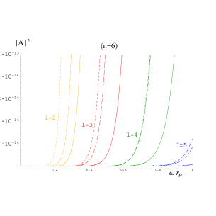
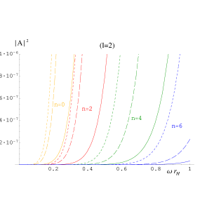
Figure 1: Absorption probability $|{\cal A}_{l}|^{2}$ for tensor (solid lines), vector (short-dashed lines) and scalar (long-dashed lines) gravitational perturbations in the bulk for: (a) $n=6$, and $l=2,3,4,5$, and (b) $l=2$, and $n=0,2,4,6$.

In Figs. 1(a) and (b), we depict the absorption probability for all types of gravitational perturbations, as a function of the dimensionless energy parameter $\omega r_{H}$, and for different values of the angular momentum number $l$ and number of extra dimensions $n$, respectively. As expected, for all types of perturbations and values of $l$ and $n$, the absorption coefficient vanishes when the energy of the propagating particle goes to zero, while it increases with $\omega r_{H}$. This is in agreement with the classical scattering theory: the larger its energy, the more likely it is for a particle to overcome the gravitational field of the black hole and escape to infinity. Figure 1(a) reveals that, as $l$ increases, the absorption probability for all types of gravitational perturbations is suppressed, in accordance with the behaviour noticed in the entries of Table 1; although the results depicted correspond to the case $n=6$, this behaviour was found to hold for all values of $n$. For fixed $l$, on the other hand, as we may see from Fig. 1(b), $|{\cal A}_{l}|^{2}$ is found to exhibit a significant suppression also with $n$, for all types of gravitational perturbations, in agreement again with the behaviour noticed in the entries of Table 1. This behaviour is observed for the lowest two partial modes with $l=2$ and $l=3$; for higher values of $l$, $|{\cal A}_{l}|^{2}$ shows a temporary enhancement, as $n$ increases from 0 to 2, that nevertheless changes again to a rapid suppression as $n$ increases further.

As it was noticed by studying the asymptotic low-energy regime, the absorption probability for tensor gravitational perturbations is significantly suppressed, compared to the other two types, also in the extended low- and intermediate-energy regime. On the other hand, the vector and scalar perturbations may dominate one over the other for different values of $l$: as it can be seen from our figures, the vector-like gravitational perturbations predominantly dominate for low values of $l$, while the scalar-like perturbations usually take over for large values of $l$. As the higher partial waves are significantly suppressed, we are led to conclude that the vector-type perturbations will be the dominant gravitational degree of freedom to be emitted in the bulk by a Schwarzschild-like higher-dimensional black hole. However, different types of perturbations are characterized by a different multiplicity of states for the same value of $l$, and the latter must be taken into account before such conclusions can be safely drawn.

5 Energy Emission Rate

We finally turn to the energy emission rate by the higher-dimensional Schwarzschild black hole for gravitons in the bulk. Let us first address the issue of the multiplicities of states that correspond to the same angular momentum number $l$. For tensor, vector, and scalar type of perturbations these are given by the expressions [17]

$$N_{l}^{(T)}=\frac{n(n+3)(l+n+2)(l-1)(2l+n+1)(l+n-1)!}{2(l+1)!\,(n+1)!}\,,$$ (47)

$$N_{l}^{(V)}=\frac{l(l+n+1)(2l+n+1)(l+n-1)!}{(l+1)!\,n!}\,,$$ (48)

$$N_{l}^{(S)}=\frac{(2l+n+1)(l+n)!}{l!\,(n+1)!}\,,$$ (49)

respectively. As it is evident, the multiplicities depend also on the dimensionality of spacetime. In Table 3, we display the multiplicities of states for tensor, vector and scalar perturbations, for some indicative values of $l$ and $n$. We immediately observe the proliferation of states as either one of these two parameters increases, especially the one with the number of extra dimensions. It thus becomes clear that the value of the absorption probability alone will not be the only decisive factor that will determine the contribution of each type of gravitational perturbation to the total emission rate of the black hole.

$\begin{array}[]{cccc}\hline\cr\hline\cr{\rule[-5.69054pt]{0.0pt}{22.76219pt}}&\hskip 36.98866ptN_{l}^{(T)}&\hskip 36.98866ptN_{l}^{(V)}&\hskip 36.98866ptN_{l}^{(S)}\\ {\rule[-8.53581pt]{0.0pt}{22.76219pt}}&n=1\,\,\,\,\,\,\,n=6&n=1\,\,\,\,\,\,\,n=6&\hskip 5.69046ptn=1\,\,\,\,\,\,\,n=6\\ \hline\cr{\rule[-5.69054pt]{0.0pt}{19.91692pt}l=2}&10\,\,\qquad 495&16\qquad 231&9\,\qquad\,44\\ {\rule[-5.69054pt]{0.0pt}{19.91692pt}l=3}&24\qquad 2574&30\qquad 910&16\qquad 156\\ {\rule[-5.69054pt]{0.0pt}{19.91692pt}l=4}&42\qquad 8748&\,48\,\,\,\quad\,2772&25\qquad 450\\ {\rule[-5.69054pt]{0.0pt}{19.91692pt}l=5}&\,64\,\quad\,\,\,23868&\,70\,\,\,\quad\,7140&\,36\,\,\quad\,\,\,1122\\ \hline\cr\hline\cr\end{array}$

Table 3: Multiplicities of states corresponding to the same angular momentum number $l$ for tensor, vector and scalar perturbations, for $n=1$ and $n=6$.

With the multiplicities of states and values of the absorption probability for each type of perturbation at our disposal, we can now calculate the corresponding energy emission rate at the low-energy regime. The contribution of each type of gravitational perturbation to the total graviton energy emission rate is given by the expression[4]

$$\frac{d^{2}E^{(P)}}{dt\,d\omega}=\frac{1}{2\pi}\,\sum_{l}\,N_{l}^{(P)}|{\cal A}_{l}^{(P)}|^{2}\,\frac{\omega}{\exp(\omega/T_{H})-1}\,,$$ (50)

where the superscript $P=(T,V,S)$ denotes the type of perturbation, and the black hole temperature is given in Eq. (3). Summing over the three contributions, we may obtain the total amount of energy emitted per unit time and unit frequency by the black hole in the form of gravitons in the bulk. As this result would be more useful in the context of an exact numerical analysis (to which we hope to return soon), here we will concentrate on the relative emission rates for the different types of gravitational perturbations and their relative magnitude to the one for bulk scalar fields.

A simple numerical analysis, by combining Eq. (50) with the entries of Tables 1 and 3, reveals that, in the asymptotic low-energy regime, the vector-like perturbations are indeed the dominant type of gravitational degree of freedom emitted in the bulk by the black hole. For example, for $n=2$ and $l=2$, vector perturbations amount to 85% of the total gravitational degrees of freedom emitted, compared to 13% for scalar and 2% for tensor degrees. As $n$ increases further, so does the dominance of the vector-like perturbations that, for $n=6$ and $l=2$, reaches the magnitude of 97%. This dominance is never over-turned but it may be significantly decreased, at the level of higher partial waves: for instance, for $n=6$ and $l=4$, the vector, scalar and tensor perturbations correspond to 74%, 12% and 14%, respectively, of the total number of gravitational degrees of freedom emitted. In fact, due to their large multiplicity of states, the tensor perturbations dominate over the scalar ones, for most large values of $n$ and/or $l$.

Figure 2: Energy emission rates for tensor (thin solid lines), vector (short-dashed lines) and scalar (long-dashed lines) gravitational perturbations, and scalar fields (thick solid lines) in the bulk, for (a) $n=1$, and (b) $n=6$.

The above results valid at the lowest part of the radiation spectrum may change for higher values of the energy parameter. Therefore, in Figs. 2(a) and (b), we plot the energy emission rates for different types of gravitational perturbations, for $n=1$ and $n=6$, respectively, as these follow by using our complete analytical expression (32)-(33) for the absorption probability. For comparison, we also display the energy emission rate for scalar fields in the bulk. In the sum over $l$ in Eq. (50) we have included all modes up to $l=12$, although at the very low-energy part of the spectrum, the contribution of all modes with $l\geq 4$ is at least four orders of magnitude smaller than the one of the $l=2$ for every value of $n$. Having included a large enough number of modes in the sum, allows for deviations from this behaviour as the energy increases.

The results depicted in Fig. 2 are in fact in excellent agreement with the conclusions derived by using the simplified expression for $|{\cal A}_{l}|^{2}$. The vector-type perturbations are indeed the dominant gravitational degrees of freedom to be emitted by the black hole in the bulk for every value of $n$. What depends on the number of extra dimensions is the relative magnitude of the energy emission rate of scalar and tensor perturbations: whereas for low $n$, the tensor perturbations are subdominant to the scalar ones over the entire low-energy regime, for high $n$, they clearly dominate over the latter ones. Despite the above, the energy emission rates for all types of gravitational perturbations in the bulk, even when combined, remain well below the one for scalar fields in the low-energy regime. This is due to the fact that the emission rate for scalar fields receives a significant enhancement, in this particular energy regime, from the dominant $l=0$ and $l=1$ modes, that are absent from the spectrum of gravitational perturbations. As the energy parameter increases though, we expect the higher partial waves to gradually come into dominance and possibly help gravitons to dominate over the bulk scalar fields.

By comparing finally the vertical axes of the two plots in Fig. 2, we conclude that the low-energy emission rate for all types of degrees of freedom in the bulk decreases as the number of extra dimensions increases. Although both the temperature of the black hole and multiplicity of states undergo a significant enhancement as $n$ increases, the equally significant suppression of the absorption probability, depicted in Fig. 1(b), prevails, leading to the suppression of the number of degrees of freedom emitted by the black hole. This low-energy suppression for bulk scalar fields was first seen in [7, 9] but the exact numerical analysis performed in the latter work showed that, for higher values of the energy parameter, the spectrum is enhanced with the number of extra dimensions. This is caused by the milder suppression of the absorption probability with $n$ at higher frequencies, but also by the shift of the emission curve towards higher energies, in accordance with Wien’s law – the latter leads to the emission of more higher frequency particles and less low-energy ones as $n$ increases [9]. Due to the similarities observed in the behaviour of gravitational and scalar fields in the bulk, we expect the same enhancement to take place also for gravitons at higher energy regimes.

6 Conclusions

A higher-dimensional black hole created in the context of a brane-world theory will decay through the emission of Hawking radiation both in the bulk and on the brane. The type of particles emitted along each “channel” are determined by the assumptions of the particular model, with only gravitons and possibly scalars propagating in the bulk within the framework of the Large Extra Dimensions scenario. Although the emission of scalars has been studied in detail, until recently gravitons have received little attention.

In this work, we have addressed this gap in the literature by investigating the emission of tensor, vector and scalar gravitational modes in the bulk from a ($4+n$)-dimensional Schwarzschild black hole. Working in the low energy regime, we analytically solved the corresponding field equations and computed the absorption probability in each case. Both a complete analytic expression and its asymptotic low-energy simplification were studied in detail, and their dependence on the angular momentum number $l$ and number of extra dimensions $n$ was examined. Although numerically different as the energy increases, these two expressions have identical qualitative behaviours, that reveal an increase in the value of the absorption probability with increasing energy and suppression as the number of partial wave $l$ and extra dimensions $n$ increase.

The complete analytical expression for the absorption probability was then used to derive the contribution of each gravitational degree of freedom to the total graviton emission rate of the black hole in the bulk. Accounting for the rapid proliferation of state multiplicities with $l$ or $n$, a sum over the first twelve partial waves was performed to obtain the total low-energy emission rate for each gravitational degree of freedom. Our results show that vector perturbations are the dominant mode emitted in the bulk for all values of $n$. The relative emission rates of the subdominant scalar and tensor modes depend on $n$, with scalars foremost at small $n$ and tensors more prevalent at high $n$. The absence of the $l=0,1$ partial waves, dominant in the low-energy regime, from all gravitational spectra causes even the total gravitational emission rate to be subdominant to that of scalar fields in the bulk. Finally, as previously found for bulk scalar fields, the energy emission rates for all types of gravitational perturbations are suppressed with the number of extra dimensions in the entire low-energy regime.

In this work we have focused on the low-energy part of the Hawking radiation spectrum as it permitted analytical calculation and derivation of closed form expressions for the absorption probability for gravitons. Although the radiation emitted in the bulk is not directly observable, it determines the energy left for emission on our brane. In this context, our results, in addition to their theoretical interest, would be of particular use to experiments developed to detect the low-energy spectrum of radiation emitted from a higher-dimensional black hole. As the exact form of the complete gravitational spectrum is still pending, we hope to return in the near future with results from a numerical analysis that could only provide the answer to this question.

Note added in proof. While this work was at its last stages, two relevant papers appeared in the literature, [18] and [19]. In particular, the latter work [19], that studies the graviton emission rate in the bulk, overlaps with ours with respect to the analytical results for the cases of tensor and vector gravitational perturbations, which are in agreement with ours.

Acknowledgments. S.C and O.E. acknowledge PPARC and I.K.Y. fellowships, respectively. The work of P.K. is funded by the UK PPARC Research Grant PPA/A/S/ 2002/00350. This research was co-funded by the European Union in the framework of the Program $\Pi Y\Theta A\Gamma OPA\Sigma-II$ of the “Operational Program for Education and Initial Vocational Training” ($E\Pi EAEK$) of the 3rd Community Support Framework of the Hellenic Ministry of Education, funded by $25\%$ from national sources and by $75\%$ from the European Social Fund (ESF).

References

- [1] N. Arkani-Hamed, S. Dimopoulos and G. R. Dvali, Phys. Lett. B 429, 263 (1998) [hep-ph/9803315]; Phys. Rev. D 59, 086004 (1999) [hep-ph/9807344]; I. Antoniadis, N. Arkani-Hamed, S. Dimopoulos and G. R. Dvali, Phys. Lett. B 436, 257 (1998) [hep-ph/9804398].
- [2] L. Randall and R. Sundrum, Phys. Rev. Lett. (1999) 3370; Phys. Rev. Lett. (1999) 4690.
- [3] T. Banks and W. Fischler, hep-th/9906038; D. M. Eardley and S. B. Giddings, Phys. Rev. D66, 044011 (2002) [gr-qc/0201034]; H. Yoshino and Y. Nambu, Phys. Rev. D66, 065004 (2002) [gr-qc/0204060]; Phys. Rev. D67, 024009 (2003) [gr-qc/0209003]; E. Kohlprath and G. Veneziano, JHEP 0206, 057 (2002) [gr-qc/0203093]; V. Cardoso, O. J. C. Dias and J. P. S. Lemos, Phys. Rev. D 67, 064026 (2003)[hep-th/0212168]; E. Berti, M. Cavaglia and L. Gualtieri, Phys. Rev. D69, 124011 (2004) [hep-th/ 0309203]; V. S. Rychkov, Phys. Rev. D 70, 044003 (2004) [hep-ph/0401116]; S. B. Giddings and V. S. Rychkov, Phys. Rev. D 70, 104026 (2004) [hep-th/0409131]; O. I. Vasilenko, hep-th/0305067; H. Yoshino and V. S. Rychkov, Phys. Rev. D 71 (2005) 104028 [hep-th/0503171].
- [4] P. Kanti, Int. J. Mod. Phys. A 19, 4899 (2004) [hep-ph/0402168].
- [5] M. Cavaglia, Int. J. Mod. Phys. A18, 1843 (2003) [hep-ph/0210296]; G. Landsberg, Eur. Phys. J. C33, S927 (2004) [hep-ex/0310034]; K. Cheung, hep-ph/0409028; S. Hossenfelder, hep-ph/0412265; C.M. Harris, hep-ph/0502005; A. S. Majumdar and N. Mukherjee, astro-ph/0503473.
- [6] S. W. Hawking, Commun. Math. Phys. 43, 199 (1975).
- [7] P. Kanti and J. March-Russell, Phys. Rev. D 66, 024023 (2002) [hep-ph/0203223].
- [8] V. P. Frolov and D. Stojkovic, Phys. Rev. D 66, 084002 (2002) [hep-th/0206046]; Phys. Rev. D 67, 084004 (2003) [gr-qc/0211055].
- [9] C. M. Harris and P. Kanti, JHEP 0310, 014 (2003) [hep-ph/0309054].
- [10] P. Kanti, J. Grain and A. Barrau, Phys. Rev. D 71 (2005) 104002 [hep-th/0501148].
- [11] A. Barrau, J. Grain and S. O. Alexeyev, Phys. Lett. B 584, 114 (2004); J. Grain, A. Barrau and P. Kanti, hep-th/0509128.
- [12] E. l. Jung, S. H. Kim and D. K. Park, Phys. Lett. B 586 (2004) 390 [hep-th/0311036]; JHEP 0409 (2004) 005 [hep-th/0406117]; Phys. Lett. B 602 (2004) 105 [hep-th/0409145]; Phys. Lett. B 614 (2005) 78 [hep-th/0503027]; E. Jung and D. K. Park, Nucl. Phys. B 717 (2005) 272 [hep-th/0502002]; hep-th/0506204.
- [13] A. S. Cornell, W. Naylor and M. Sasaki, hep-th/0510009.
- [14] H. Kodama and A. Ishibashi, Prog. Theor. Phys. 110, 701 (2003) [hep-th/0305147].
- [15] F.R. Tangherlini, Nuovo Cimento 27, 636 (1963); R. C. Myers and M. J. Perry, Annals Phys. 172, 304 (1986).
- [16] M. Abramowitz and I. Stegun, Handbook of Mathematical Functions (Academic, New York, 1996).
- [17] M. A. Rubin and C. R. Ordonez, J. Math. Phys. 25, 2888 (1984); J. Math. Phys. 26, 65 (1985).
- [18] D. K. Park, hep-th/0512021.
- [19] V. Cardoso, M. Cavaglia and L. Gualtieri, hep-th/0512002; hep-th/0512116.