General Coordinate Transformations as the Origins of Dark Energy

Abstract

In this note we demonstrate that the algebra associated with coordinate transformations might contain the origins of a scalar field that can behave as an inflaton and/or a source for dark energy. We will call this particular scalar field the diffeomorphism scalar field. In one dimension, the algebra of coordinate transformations is the Virasoro algebra while the algebra of gauge transformations is the Kac-Moody algebra. An interesting representation of these algebras corresponds to certain field theories that have meaning in any dimension. In particular the so called Kac-Moody sector corresponds to Yang-Mills theories and the Virasoro sector corresponds to the diffeomorphism field theory that contains the scalar field and a rank-two symmetric, traceless tensor. We will focus on the contributions of the diffeomorphism scalar field to cosmology. We show that this scalar field can, qualitatively, act as a phantom dark energy, an inflaton, a dark matter source, and the cosmological constant $\Lambda$.

Keywords: coadjoint representation; dark energy; dark matter; cosmology

1 Introduction

Recently experimental cosmology has brought new challenges to the theoretical understanding of the universe. Until now, the standard hot big-bang cosmology has been very successful in explaining four important observed facts: (1) the expansion of Universe, (2) the origin of the cosmic background radiation, (3) the nucleosynthesis of the light elements, (4) the formation of galaxies and the large scale structure of Universe. However, recent discoveries from Supernova Cosmology Project [References] and WMAP [References] strongly suggest that the standard cosmology needs to be revised. This new standard cosmology must now explain

$$\ \circ\ \ \mbox{Flat and accelerating Universe}$$

$$\ \circ\ \ \mbox{Rapid expansion of Universe in early period (Inflation)}$$

$$\ \circ\ \ \mbox{Composition of Universe: 73\% dark energy; 23\% dark matter; 4\% baryons\thinspace}$$

The theoretical search for this new standard cosmology is very active and there is an overwhelming amount of literature published where most of them have the same theme: scalar fields. In this work we ask if there is a guiding principle that might account for the presence of new fields in cosmology. We posit that there is a symmetry that can accompany general relativity in providing an explanation for some of the new features found in cosmology. This symmetry is not new and is already exploited in general relativity through general coordinate covariance. However we will realize the symmetry using an approach used in string theory. Since string theories are two dimensional field theories, direct contributions to gravity coming from curvature and the Einstein-Hilbert action are diminished because of the low dimension. In fact in two dimensions the Einstein-Hilbert action can at most distinguish different topological structures. Our starting principle will be the algebra of Lie derivatives which exists in any dimension including one dimension. We will show that this algebra admits a field theoretic representation analogous to the Yang-Mills gauge potentials that arise from the algebra of gauge transformations.

In one dimension, this field theory comes from the coadjoint representation [References,References,References,References] of the one dimensional algebra of Lie derivatives called the Virasoro algebra. In string theory this representation is used to understand the geometric origin of gravitational anomalies. As we will review here, one can understand the origins of two dimensional gauge and gravitational anomalies through the Geometric Action [References,References,References,References,References] as well as establishes the Lagrangian for the fields living in the coadjoint representation called the Transverse Action [References,References]. For this work, the importance feature of the Transverse Action as compared to the Geometric Action is that the Transverse Action can exist in any dimension. We will review the construction of the Transverse Action with both the algebra of gauge and coordinate transformations. We show that there is a naturally occurring scalar fields called the diffeomorphism scalar field (diff scalar) that arises naturally from the algebra of associated with coordinate transformations.

As a matter of completeness we will keep this paper somewhat self contained and outline of this paper as follows. We will first review the Robertson-Walker cosmology and as well as four of the more popular scalar field theories discussed in the literature. This will introduce our notation to the reader and put this work in a more familiar setting. In the next section we discuss the method we use at arriving at the Lagrangian for the diff scalar. We are then able to discuss the cosmological implications of the diffeomorphism scalar field by combining the action for the diff scalar with the Einstein-Hilbert action in the next section. We show that the diff scalar field can, qualitatively, act as phantom dark energy, an inflaton, a dark matter source, and the cosmological constant $\Lambda$.

2 Standard Cosmology Review

The standard cosmology is based on two postulates that Universe is homogeneous and isotropic at large scales [References,References,References]. These postulates are strongly supported by the cosmic microwave background (CMB) radiation coming from various regions of sky: the temperature of the CMB radiation from different parts of sky are almost identical. These postulates are called the cosmological principle. With proper choice of coordinates these symmetry postulates thus allow us to write the metric in the form of Robertson-Walker metric:

$$ds^{2}=-dt^{2}+a^{2}\left(t\right)\left\{{dr^{2}\over 1-kr^{2}}+r^{2}\left(d\theta^{2}+\sin^{2}\theta\mbox{ }d\phi^{2}\right)\right\}$$ (1)

Here we used the convention: $\hbar=c=1$. The function $a\left(t\right)$ is called the scale factor of the universe (cosmic scale factor). Rescaling this factor appropriately, the constant $k$ can be always taken to be $0$, $+1$, or $-1$:

$$\ k=+1:\mbox{ closed universe with positive spatial curvature}$$

$$\ k=0:\mbox{ flat universe with zero spatial curvature}$$

$$\ k=-1:\mbox{ open universe with negative spatial curvature}$$

Since current observations seems to prefers a flat universe, we will adopt $k=0$ throughout this paper. The cosmological principle also demands that all cosmic tensors are maximally form-invariant with respect to the spatial coordinates. As a consequence of this constraint the most general form-invariant tensor for the energy-momentum tensor is given by:

$$T_{00}=\rho\left(t\right),\ \ \ T_{0i}=0,\ \ \ T_{ij}=p\left(t\right)g_{ij},\ \ \ \ \ \ i,j=1,2,3$$ (2)

where $\rho\left(t\right)$ and $p\left(t\right)$ are arbitrary functions that depend only on time. Rewriting the energy-momentum tensor as

$$T_{\mu\nu}=\left(\rho+p\right)U_{\mu}U_{\nu}+pg_{\mu\nu}$$ (3)

where $U_{\mu}$ is a “four-velocity vector”

$$U^{0}=1,\mbox{ \thinspace\thinspace\thinspace\thinspace\thinspace\thinspace\thinspace\thinspace\thinspace\thinspace\thinspace}U^{i}=0\mbox{ \thinspace}\left(i=1,2,3\right)$$ (4)

we identify $\rho\left(t\right)$ and $p\left(t\right)$ as with energy density and pressure of a perfect fluid.

Using this form of the energy-momentum tensor and the Robertson-Walker metric, we obtain the Friedmann equations from Einstein’s field equations:

$$H^{2}\left(t\right) = {\rho\left(t\right)\over 3M_{pl}^{2}}+{\Lambda\over 3}-{k\over a^{2}\left(t\right)}$$ (5)

$$\dot{H}\left(t\right) = {dH\left(t\right)\over dt}=-{1\over 2M_{\rm pl}^{2}}\left(\rho\left(t\right)+p\left(t\right)\right)+{k\over a^{2}\left(t\right)}$$ (6)

where the Hubble parameter $H(t)$ is defined as

$$H(t)={\dot{a}\left(t\right)\over a\left(t\right)}$$ (7)

and

$$M_{\rm pl}=\mbox{\mbox{reduced Planck mass}}=\left(8\pi G\right)^{-1/2}.$$ (8)

From the energy-momentum conservation condition $\nabla_{\mu}T^{\mu 0}=0$ we find

$$\dot{\rho}+3H\left(\rho+p\right)=0.$$ (9)

This equation and the Friedmann equations are not independent from each other. The equation of state, the pressure-to-energy density ratio, is defined as

$$w={p\over\rho}.$$ (10)

Typical values of $w$ are

Radiation: $$w={\textstyle{1\over\vphantom{2}\smash{\raise 0.60275pt\hbox{$\scriptstyle{3}$}}}}$$ (11)

Matter: $$w=0$$ (12)

Cosmological constant: $$w=-1.$$ (13)

The condition for the accelerating expansion of Universe can be given in several ways:

the cosmic scale factor is accelerating : $$\mbox{\ \ \ \ \ }\ddot{a}>0$$

the comoving Hubble length is decreasing : $$\mbox{\ \ \ \ }{d\over dt}\left({H^{-1}(t)\over a(t)}\right)<0$$ (14)

negative Pressure : $$\mbox{\ \ \ }\rho\left(t\right)+3p\left(t\right)<0.$$

The last condition can be also expressed by using the equation of state:

$$w<-{\textstyle{1\over\vphantom{2}\smash{\raise 0.60275pt\hbox{$\scriptstyle{3}$}}}}.$$ (15)

2.1 Single-Field Inflation Model

The inflation models assume an era of inflation during the Big Bang, in which the energy density of the Universe was dominated by the potential energy of the scalar fields (inflatons). The inflation is defined as any epoch during which the conditions Eq.14 are satisfied and used for the events in early Universe. The negative pressure condition for the inflation model motivates one to introduce a scalar field (inflaton) with its Lagrangian density given by

$$\mathcal{L}_{\phi}={\textstyle{1\over\vphantom{2}\smash{\raise 0.60275pt\hbox{$\scriptstyle{2}$}}}}g^{\mu\nu}\left(\partial_{\mu}\phi\right)\left(\partial_{\nu}\phi\right)-V\left(\phi\right).$$ (16)

The term $V\left(\phi\right)$ is the potential of the scalar field and the choice of its form characterizes the types of inflationary models. Using the above Lagrangian density we have

$$T^{\mu\nu}=\left(\partial^{\mu}\phi\right)\left(\partial^{\nu}\phi\right)-g^{\mu\nu}\left[{\textstyle{1\over\vphantom{2}\smash{\raise 0.60275pt\hbox{$\scriptstyle{2}$}}}}\left(\partial^{\lambda}\phi\right)\left(\partial_{\lambda}\phi\right)+V\left(\phi\right)\right]$$ (17)

or

$$\rho={\textstyle{1\over\vphantom{2}\smash{\raise 0.60275pt\hbox{$\scriptstyle{2}$}}}}\dot{\phi}^{2}+{\textstyle{1\over\vphantom{2}\smash{\raise 0.60275pt\hbox{$\scriptstyle{2}$}}}}\left(\nabla_{i}\phi\right)^{2}+V\left(\phi\right)$$ (18)

and

$$p={\textstyle{1\over\vphantom{2}\smash{\raise 0.60275pt\hbox{$\scriptstyle{2}$}}}}\dot{\phi}^{2}-{\textstyle{1\over\vphantom{2}\smash{\raise 0.60275pt\hbox{$\scriptstyle{6}$}}}}\left(\nabla_{i}\phi\right)^{2}-V\left(\phi\right).$$ (19)

The equation of motion for the scalar field is given by

$$\ddot{\phi}+3H\dot{\phi}-{1\over a^{2}\left(t\right)}\vec{\nabla}^{2}\phi=-{\partial V\over\partial\phi}.$$ (20)

2.2 Quintessence

In quintessence $Q$ is a scalar field that is introduced to explain the accelerating Universe. Quintessence is a dynamical field and generally has a time-varying, spatially inhomogeneous negative pressure [References]. The Lagrangian for the quintessence is given by

$$\mathcal{L}={\textstyle{1\over\vphantom{2}\smash{\raise 0.60275pt\hbox{$\scriptstyle{2}$}}}}\partial_{\mu}Q\partial^{\mu}Q-V\left(Q\right).$$ (21)

The energy density and pressure of quintessence are, then, respectively,

$$\rho={\textstyle{1\over\vphantom{2}\smash{\raise 0.60275pt\hbox{$\scriptstyle{2}$}}}}\dot{Q}^{2}+V\left(Q\right),\ \ \ \ p={\textstyle{1\over\vphantom{2}\smash{\raise 0.60275pt\hbox{$\scriptstyle{2}$}}}}\dot{Q}^{2}-V\left(Q\right).$$ (22)

It is easy to see that the ratio of the pressure to the energy density, $w$, is $-1<w\leq 0$ for quintessence. A particular class of quintessence models have a tracker behavior. In these models the density of quintessence closely tracks the radiation density until the equality between matter and radiation is established. Once the matter-radiation equality is established the quintessence start to behave as dark energy. k-essence and phantom energy are the special cases of quintessence.

2.3 k-essence

The idea of k-essence (or k-inflation) was originally introduced as a possible model for inflation [References]. In this model an inflationary evolution of the early universe is driven by non-quadratic kinetic energy terms starting from rather arbitrary initial conditions instead of the potential energy term $V\left(\varphi\right)$. When the idea of k-essence is applied to the coincidence problem, it was shown that [References, References] k-essence can act as a dynamical attractor at the onset of matter domination period and introduce the cosmic acceleration at present time. A purely kinetic k-essence model was investigated in [References]. In this investigation the author showed that k-essence in this model can evolve like the sum of a dark matter component and a dark energy component if the Lagrangian for the k-essence has a local extremum.

The Lagrangian for a typical k-essence model is given as the pressure of the k-essence:

$$\mathcal{L}=P=V\left(\phi\right)F\left(X\right),$$ (23)

where $\phi$ is the scalar field representing k-essence, and $X$ is defined as

$$X={\textstyle{1\over\vphantom{2}\smash{\raise 0.60275pt\hbox{$\scriptstyle{2}$}}}}\partial_{\mu}\phi\partial^{\mu}\phi.$$ (24)

The pressure in this model is given by the Lagrangian itself, while the energy density is given by

$$\rho=V\left(\phi\right)\left[2XF_{X}-F\right]$$ (25)

where

$$F_{x}={dF\over dX}.$$ (26)

Using these pressure and energy density, we have the ratio of the pressure to the energy density, $w$, as

$$w={F\over 2XF_{X}-F}.$$ (27)

The behavior of this ratio is determined by the form of $V\left(\phi\right)$ and $F\left(X\right)$.

2.4 Phantom Dark Energy

The phantom dark matter is a special case of quintessence characterized by the ratio of the pressure to the energy density, $w<-1$. Though the dark energy with $w<-1$ will violate all energy conditions [References], the dark energy models with $w<-1$ that are consistent with observed data can be constructed [References]. A phenomenological model of phantom dark energy can be constructed to give new insight to the coincident problem through the interaction of the phantom dark energy with dark energy and dark matter [References].

3 The Origin of the Diffeomorphism Field

In this work we posit that there exist a scalar field, the diffeomorphism scalar field, that has its origins in one of the most primitive symmetries used in physics; general coordinate covariance. When coupled to a Robertson-Walker metric, this scalar field qualitatively exhibits the behavior of an inflaton, phantom dark energy and the cosmological constant [References]. Here we review the construction of the Lagrangian for the diffeomorphism field. We will marry the general coordinate transformations with gauge transformations to show the analogy with the vector potential in Yang-Mills theories.

Recall that under a general coordinate transformation, tensors transform as

$$A^{\prime}_{a}(x^{\prime}) = \left({\partial x^{b}\over\partial x^{\prime a}}\right)A_{b}(x)$$ (28)

$$A^{\prime a}(x^{\prime}) = \left({\partial x^{\prime a}\over\partial x^{\prime b}}\right)A^{b}(x).$$ (29)

Their infinitesimal counterpart, i.e. $x^{\prime a}=x^{a}+\xi^{a}$, where $\xi$ is vector field, determine the Lie derivative;

$${\cal L}_{\xi}A_{a}(x) = -\xi(x)^{b}\partial_{b}A_{a}(x)-A_{b}(x)\partial_{a}\xi^{b}(x)$$ (30)

$${\cal L}_{\xi}A^{a}(x) = -\xi(x)^{b}\partial_{b}A^{a}(x)+A^{b}(x)\partial_{b}\xi^{a}(x).$$ (31)

It is important to note that for tensors the Lie derivative is independent of the connection, $\nabla_{a}$. Thus the field theory associated with diffeomorphisms will be independent of Riemannian curvature.

The analogue of the above for finite and infinitesimal transformations for gauge transformations on a (non-Abelian) vector potential are

$$V^{\prime}_{a}(x)=U(x)V_{a}(x)U(x)^{-1}+iU(x)\partial_{a}U(x)^{-1}$$ (32)

and

$$\delta_{\Lambda}V_{a}(x)=i\left[\Lambda(x),V_{a}(x)\right]-\partial_{a}\Lambda(x),$$ (33)

where $U(x)=\exp{i\Lambda(x)}$ is the finite gauge transformation generated by $\Lambda(x)$.

3.1 The Adjoint Representation

The vector fields ($\xi^{a}$) and gauge parameters ($\Lambda$) act on themselves and form the adjoint representation. The gauge and coordinate transformations in one dimension are particularly interesting because the dual representation of the adjoint representation, called the coadjoint representation, reveals the gauge and gravitational anomalies that appear in two dimensional field theories and string theories. Interestingly enough, the coadjoint representation appears to come from a field theory that need not be constrained to two dimensions. In the case of the gauge transformations, that field theory is Yang-Mills.

To see how these field theories comes about, lets begin by marrying the one dimensional infinitesimal coordinate transformations (Lie derivatives) and infinitesimal gauge transformations together. This marriage is the semi-direct product of the Virasoro algebra [References], which corresponds to Lie derivatives of one dimensional vector fields, and an SU(N) Kac-Moody algebra, which corresponds to SU(N) gauge transformations on a circle or a line. This algebra admits central extensions (or phases at the group level) so that the basic elements of this algebra contains the Lie derivative generated by the one dimensional vector field $\xi^{a}(\theta)$, a gauge parameter $\Lambda(\theta)$, and a constant, say $a$ so we can have a three-tuple $\left({\xi};\Lambda;a\right)$. Then the commutation relations, $[[*,*]]$ for the adjoint representation is

$$[[({\xi};\,\Lambda;\,a),({\eta};\Xi;\,b)]]=({\xi\circ\eta};\,-\xi^{b}\partial_{b}\Xi+\eta^{b}\partial_{b}\Lambda+[\Lambda,\Xi];\,\left\{\Lambda,\Xi,\xi,\eta\right\}),$$ (34)

where the central extensions $\left\{\Lambda,\Xi,\xi,\eta\right\}$ is given by

$$\left\{\Lambda,\Xi,\xi,\eta\right\} = {\textstyle{k\over\vphantom{2}\smash{\raise 0.60275pt\hbox{$\scriptstyle{2\pi}$}}}}\int(\Lambda\partial_{a}\Xi-\Xi\partial_{a}\Lambda)d\,\theta^{a}+{\textstyle{c\over\vphantom{2}\smash{\raise 0.60275pt\hbox{$\scriptstyle{2\pi}$}}}}\int(\xi^{a}\nabla_{a}\nabla_{b}\nabla_{c}\eta^{c})\,d\theta^{b}\,\,\,\,$$

$$+ {\textstyle{h\over\vphantom{2}\smash{\raise 0.60275pt\hbox{$\scriptstyle{2\pi}$}}}}\int(\xi^{a}\nabla_{a}\eta_{b})\,d\theta^{b}-(\xi\leftrightarrow\eta).$$

The parameter $h$,$k$, and $c$ are arbitrary constants that define the central extension. The new vector field $(\xi\circ\eta)^{a}$ is defined through the Lie derivative,

$$(\xi\circ\eta)^{a}\equiv{\cal L}_{\xi}\eta^{a}=-\xi^{b}\partial_{b}\eta^{a}+\eta^{b}\partial_{b}\xi^{a}.$$ (36)

3.2 The Coadjoint Representation

Associated with the adjoint representation, we can define its dual by writing an invariant product [References,References] . Let $\left(\eta;\Xi;\,b\right)$ be an element of the adjoint and ${\cal B}=\left(D,A,\mu\right)$ be an element of the algebra’s dual. Then the one dimensional line integral gives an invariant pairing:

$$\left\langle\left(D,A,\mu\right)\mid\left(\eta;\Xi;\,b\right)\right\rangle=\int\left(D_{ab}(\theta)\xi^{a}(\theta)+A_{b}(\theta)\Lambda(\theta)\right)\,d\theta^{b}+b\,\mu.$$ (37)

Demanding that the pairing to be invariant under gauge and coordinate transformations is equivalent to acting on the pairing with an adjoint element and getting zero. Consider the action of the adjoint element ${\cal F}=\left(\xi\left(\theta\right),\Lambda\left(\theta\right),a\right)$ on the pairing. Then the invariance of the pairing

$$\delta_{\cal F}\left\langle\left(D,A,\mu\right)\mid\left(\eta;\Xi;\,b\right)\right\rangle=0$$ (38)

and Leibnitz rule implies that

$$\delta_{\mathcal{F}}B=\left(\delta_{\cal F}D\left(\theta\right),\delta_{\cal F}A\left(\theta\right),0\right)$$ (39)

where

$$\delta_{\cal F}{\rm D}\left(\theta\right)=\;\stackrel{{\scriptstyle\rm shift\;in\;the\;diff\;coadjoint\;element}}{{{}{}{\overbrace{\mathrel{\mathop{\underbrace{2\xi^{{}^{\prime}}{\rm D}+{\rm D}^{{}^{\prime}}\xi+{\textstyle{c\mu\over\vphantom{2}\smash{\raise 0.60275pt\hbox{$\scriptstyle{2\pi}$}}}}\xi^{\prime\prime\prime}+{\textstyle{h\mu\over\vphantom{2}\smash{\raise 0.60275pt\hbox{$\scriptstyle{2\pi}$}}}}\xi^{\prime}}}\limits_{coordinate\ trans}}-\mathrel{\mathop{\underbrace{Tr\left({\rm A}\Lambda^{\prime}\right)}}\limits_{gauge\ trans}}}}}}$$ (40)

and

$$\delta_{\cal F}{\rm A(\theta)}=\;\stackrel{{\scriptstyle\rm shift\;in\;the\;gauge\;coadjoint\;element}}{{\,\overbrace{\mathrel{\mathop{\underbrace{{\rm A}^{\prime}\xi+\xi^{\prime}{\rm A}}}\limits_{coord\ trans}}-\mathrel{\mathop{\,\underbrace{[\Lambda\,{\rm A}-{\rm A\,}\Lambda]+k\,\mu\,\Lambda^{\prime}}}\limits_{gauge\ trans}}}}}.$$ (41)

We have suppressed the tensor indices for the fields $D_{ab}$ and $A_{b}$ and ^′ denotes $\partial_{\theta}$.

3.3 The Geometric Action

The fields $A$ in the coadjoint representation correspond to the spatial components of a gauge field while $D$ is the space-space component of a rank two tensor called the diffeomorphism field. The “$\mu$” is the central extension. Now there are two distinct Lagrangians that one can construct using the structure of the coadjoint representation. The first is called the Geometric Lagrangian.

In the geometric Lagrangian or geometric action [References, References] the coadjoint elements serve as background fields while the coordinate and group transformations become the dynamical fields. There one considers a two parameter family of coordinate and gauge transformations that can act on a fixed element of the coadjoint representation, say ${\cal B}=\left(D\left(\theta\right),A\left(\theta\right),\tilde{\mu}\right)$. The two parameters, say $\lambda$ and $\tau$, correspond to a natural coordinatization of the orbit of ${\cal B}$. The orbit of ${\cal B}$ is defined to simply be all gauge fields and diffeomorphism fields that are related to ${\cal B}$ via gauge and coordinate transformation.

On the orbit of any coadjoint element, there exist a natural symplectic structure [References] corresponding to a rank two antisymmetric tensor [References,References]. When integrated on a two-manifold this will give the geometric action. To find the geometric action for our case, namely the semi-direct product of the Virasoro and Kac-Moody groups, we define two adjoint vectors corresponding to changes in directions corresponding to coordinates $\lambda$ and $\tau$ on the orbit. These adjoint vectors are $u_{\lambda}$ and $u_{\tau}$. Now let $g$ represent the group action of both an arbitrary gauge transformation, $U(\theta,\lambda,\tau)$, and coordinate transformation, $s(\theta,\lambda,\tau)$. We denote by $Ad(g)$ the action of these gauge and coordinate transformations of the adjoint representation and $Ad^{\ast}(g)$ the group action on coadjoint elements. Then using two adjoint elements corresponding to changes in the $\lambda$ and $\tau$ directions and a coadjoint representation $w_{g}$ defined by

$$u_{\lambda} = \left(\xi_{\lambda}\left(\theta\right),\Lambda_{\lambda}\left(\theta\right),a_{\lambda}\right)$$

$$u_{\tau} = \left(\xi_{\tau}\left(\theta\right),\Lambda_{\tau}\left(\theta\right),a_{\tau}\right)$$ (42)

$$w_{g} = Ad^{\ast}\left(g\right)w=Ad^{\ast}\left(g\right)\left(D\left(\theta\right),A\left(\theta\right),\tilde{\mu}\right).$$

We then pair these elements via $\left\langle w_{g}\ |\ \left[u_{\lambda},u_{\tau}\right]\right\rangle$ to define a natural symplectic two form in the coordinates of $\lambda$ and $\tau$. This is given by

$$\left\langle w_{g}\ |\ \left[u_{\lambda},u_{\tau}\right]\right\rangle=\left\langle Ad^{\ast}\left(g\right)w\ |\ \left[u_{\lambda},u_{\tau}\right]\right\rangle=\left\langle w\ |\ \left[Ad\left(g^{-1}\right)u_{\lambda},Ad\left(g^{-1}\right)u_{\tau}\right]\right\rangle$$ (43)

Concretely we have

$$\xi_{\lambda}\left(\theta\right)=\left(\partial_{\lambda}s\left(\theta\right)\right)\circ s^{-1}\ \ \ \ \ \ \mbox{and}\ \ \ \ \ \ \Lambda_{\lambda}\left(\theta\right)=\left(\partial_{\lambda}U\right)\circ U^{-1},$$ (44)

and we find

$$Ad\left(g^{-1}\right)\xi_{\lambda}\left(\theta\right) = s^{-1}\circ\left(\partial_{\lambda}s\left(\theta\right)\right)=\partial_{\lambda}\theta={\textstyle{\partial_{\lambda}s\over\vphantom{2}\smash{\raise 0.60275pt\hbox{$\scriptstyle{\partial_{\theta}s}$}}}}$$ (45)

$$Ad\left(g^{-1}\right)\Lambda_{\lambda}\left(\theta\right) = U^{-1}\circ\left(\partial_{\lambda}U\right)=U^{-1}\partial_{\lambda}U.$$ (46)

Then in Eq.(43) we can write

$$\left[Ad\left(g^{-1}\right)u_{\lambda},Ad\left(g^{-1}\right)u_{\tau}\right]=$$

$$\left[\left({\textstyle{\partial_{\lambda}s\over\vphantom{2}\smash{\raise 0.60275pt\hbox{$\scriptstyle{\partial_{\theta}s}$}}}},U^{-1}\partial_{\lambda}U,a_{\lambda}\right),\left({\textstyle{\partial_{\tau}s\over\vphantom{2}\smash{\raise 0.60275pt\hbox{$\scriptstyle{\partial_{\theta}s}$}}}},U^{-1}\partial_{\tau}U,a_{\tau}\right)\right]=$$ (47)

$$\left(\left[{\textstyle{\partial_{\lambda}s\over\vphantom{2}\smash{\raise 0.60275pt\hbox{$\scriptstyle{\partial_{\theta}s}$}}}},{\textstyle{\partial_{\tau}s\over\vphantom{2}\smash{\raise 0.60275pt\hbox{$\scriptstyle{\partial_{\theta}s}$}}}}\right],\left[{\textstyle{\partial_{\lambda}s\over\vphantom{2}\smash{\raise 0.60275pt\hbox{$\scriptstyle{\partial_{\theta}s}$}}}},U^{-1}\partial_{\tau}U\right]+\left[U^{-1}\partial_{\lambda}U,{\textstyle{\partial_{\tau}s\over\vphantom{2}\smash{\raise 0.60275pt\hbox{$\scriptstyle{\partial_{\theta}s}$}}}}\right]+\left[U^{-1}\partial_{\lambda}U,U^{-1}\partial_{\tau}U\right],c_{V}+c_{K}\right)$$

where $c_{V}$ and $c_{K}$ are the central terms due to the commutation relations for the Virasoro and Kac-Moody algebras, respectively. Choosing $c=-h$ [References] , the central term for the Virasoro commutator is given by

$$c_{V}={\textstyle{c\over\vphantom{2}\smash{\raise 0.60275pt\hbox{$\scriptstyle{24\pi}$}}}}\int_{0}^{2\pi}d\sigma u^{\prime}v^{\prime\prime}$$ (48)

where $u={\textstyle{\partial_{\lambda}s\over\vphantom{2}\smash{\raise 0.60275pt\hbox{$\scriptstyle{\partial_{\theta}s}$}}}}$ and $v={\textstyle{\partial_{\tau}s\over\vphantom{2}\smash{\raise 0.60275pt\hbox{$\scriptstyle{\partial_{\theta}s}$}}}}$, whereas the Kac-Moody commutator gives

$$c_{k}={\textstyle{k\over\vphantom{2}\smash{\raise 0.60275pt\hbox{$\scriptstyle{2\pi}$}}}}\int_{0}^{2\pi}d\sigma Tr\left(uv^{\prime}\right),$$ (49)

where $u=U^{-1}\partial_{\lambda}U$ and $v=U^{-1}\partial_{\tau}U$. Hence, after some calculations, the geometric action

$$S_{V\otimes KM}=\int d\lambda d\tau\left\langle w\ |\ \left[Ad\left(g^{-1}\right)u_{\lambda},Ad\left(g^{-1}\right)u_{\tau}\right]\,\right\rangle$$ (50)

becomes [References,References,References,References]

$$S ={\textstyle{1\over\vphantom{2}\smash{\raise 0.60275pt\hbox{$\scriptstyle{2\pi}$}}}}\mathrel{\mathop{\underbrace{\int d^{\;2}\theta\;{\rm D}\left(\theta\right)\left({\textstyle{\partial_{\tau}s\over\vphantom{2}\smash{\raise 0.60275pt\hbox{$\scriptstyle{\partial_{\theta}s}$}}}}\right)}}\limits_{\mbox{\small{Metric \,Coupling}}}}$$

$$+ {\textstyle{1\over\vphantom{2}\smash{\raise 0.60275pt\hbox{$\scriptstyle{2\pi}$}}}}{\int d^{\;3}\theta\;\mbox{Tr}{\rm A}\left(\theta\right)\left({\textstyle{\partial_{\lambda}s\over\vphantom{2}\smash{\raise 0.60275pt\hbox{$\scriptstyle{\partial_{\theta}s}$}}}}\partial_{\theta}\left(U^{-1}\partial_{\tau}U\right)\right)}$$

$$- {\textstyle{1\over\vphantom{2}\smash{\raise 0.60275pt\hbox{$\scriptstyle{2\pi}$}}}}\int d^{\;3}\theta\;\mbox{Tr}{\rm A}(\theta){\left({\textstyle{\partial_{\tau}s\over\vphantom{2}\smash{\raise 0.60275pt\hbox{$\scriptstyle{\partial_{\theta}s}$}}}}\partial_{\theta}\left(U^{-1}\partial_{\lambda}U\right)+\left[U^{-1}\partial_{\lambda}U,U^{-1}\partial_{\tau}U\right]\right)}$$

$$- {\beta c\over 48\pi}{\int d^{\;2}\theta\;\left({\partial_{\theta}^{2}s\over\left(\partial_{\theta}s\right)^{2}}\partial_{\tau}\partial_{\theta}s-{\left(\partial_{\theta}^{2}s\right)^{2}\over\left(\partial_{\theta}s\right)^{3}}\partial_{\tau}s\right)}$$

$$- {\beta k\over 4\pi}{\int d^{\;3}\theta\;{\rm Tr}\left(U^{-1}\partial_{\theta}UU^{-1}\partial_{\tau}U\right)}$$

$$+ {{\beta k\over 4\pi}\int d^{\;3}\theta\;\mbox{Tr}\left(\left[U^{-1}\partial_{\theta}U,U^{-1}\partial_{\lambda}U\right]U^{-1}\partial_{\tau}U\right)},$$

where the measures $d^{\;2}\theta=d\theta d\tau$ and $d^{\;3}\theta=d\theta d\tau d\lambda$.

The fourth summand is recognized as the Liouville-Polyakov action [References] while the fifth and sixth terms are the Wess-Zumino-Novikov-Witten actions [References]. In the summand called the “Metric Coupling”, one sees that the diffeomorphism field interacts with the metric through

$${\rm D}\left(\theta\right)\left({\textstyle{\partial_{\tau}s\over\vphantom{2}\smash{\raise 0.60275pt\hbox{$\scriptstyle{\partial_{\theta}s}$}}}}\right)\rightarrow\sqrt{h}D_{ab}h^{ab},$$

where $h_{ab}$ is the two dimensional induced metric. This interaction is the first ingredient we will need to discuss cosmology. When the trace of $D_{ab}$ becomes constant, this term in the Lagrangian will appear as a cosmological constant.

3.4 Transverse Actions

Every point on the coadjoint orbit of ${\cal B}=\left(D,A,\mu\right)$ corresponds to a group element, $s(\theta)$ and $U(\theta)$. There are, however, group elements that do not appear on the orbit because they do not change ${\cal B}=\left(D,A,\mu\right)$. These group elements are generated by the isotropy algebra of the coadjoint element, ${\cal B}=\left(D,A,\mu\right)$. An adjoint element ${\cal F}$ belongs to the isotropy algebra of ${\cal B}=\left(D,A,\mu\right)$ when

$$\delta_{\cal F}{\rm D}\left(\theta\right)=\;{{}{}{2\xi^{{}^{\prime}}{\rm D}+{\rm D}^{{}^{\prime}}\xi+{\textstyle{c\mu\over\vphantom{2}\smash{\raise 0.60275pt\hbox{$\scriptstyle{2\pi}$}}}}\xi^{\prime\prime\prime}+{\textstyle{h\mu\over\vphantom{2}\smash{\raise 0.60275pt\hbox{$\scriptstyle{2\pi}$}}}}\xi^{\prime}-{{\rm Tr}\left({\rm A}\Lambda^{\prime}\right)}}}=0$$ (52)

and

$$\delta_{\cal F}{\rm A(\theta)}=\;{\rm A}^{\prime}\xi+\xi^{\prime}{\rm A}-{[\Lambda\,{\rm A}-{\rm A\,}\Lambda]+k\,\mu\,\Lambda^{\prime}}=0.$$ (53)

These adjoint elements are candidates for the conjugate momenta of the fields $D$ and $A$ that appear in ${\cal B}=\left(D,A,\mu\right)$. To see this recall that in Yang-Mills theories the finite gauge transformations are given by

$$A_{i}\left(x\right) \rightarrow U\left(x\right)A_{i}\left(x\right)U^{-1}\left(x\right)-\left(\partial_{i}U\left(x\right)\right)U^{-1}\left(x\right)$$ (54)

$$E^{i}\left(x\right) \rightarrow U\left(x\right)E^{i}\left(x\right)U^{-1}\left(x\right).$$ (55)

In temporal gauge

$$A_{0}=0,$$ (56)

the residual gauge transformation are time-independent gauge transformations. The infinitesimal residual gauge transformations are:

$$\delta A_{ai}\left(x\right) = \left[\Lambda\left(x\right),A\left(x\right)\right]_{ai}-\partial_{i}\Lambda_{a}\left(x\right)$$ (57)

$$\delta E_{a}^{i}\left(x\right) = \left[\Lambda\left(x\right),E\left(x\right)\right]_{a}^{i}.$$ (58)

The isotropy algebras are given by setting these equations to zero:

$$\delta_{\Lambda}A_{ai}\left(x\right) = \left[\Lambda\left(x\right),A\left(x\right)\right]_{ai}-\partial_{i}\Lambda_{a}\left(x\right)=0$$ (59)

$$\delta_{\Lambda}E_{a}^{i}\left(x\right) = \left[\Lambda\left(x\right),E\left(x\right)\right]_{a}^{i}=0.$$ (60)

In Eq.(54) and Eq.(55), the transformation laws reveal that in one space and one time dimensions, the gauge potential is in the coadjoint representation while its conjugate momentum, the electric field, is in the adjoint representation. Because $E_{i}$ is in the adjoint algebra it can gauge transform $A_{i}$. The Gauss law constraints

$$\nabla_{i}E_{a}^{i}\left(x\right)=\partial_{i}E_{a}^{i}\left(x\right)+\left[A_{i}\left(x\right),E^{i}\left(x\right)\right]_{a}=0,$$ (61)

forbids this from happening. From Eq.(59) we see that the conjugate momentum to the coadjoint element is an element of the isotropy algebra. With this one now has a way of finding a Lagrangian that will give dynamics to the fields in ${\cal B}$. We construct a Lagrangian where one of the field equations reduces to a Gauss Law constraint which corresponds to the isotropy equation in two dimensions. The Lagrangian can exist in any dimension. For the Kac-Moody sector the Lagrangian is the familiar:

$$S_{YM}=-{\textstyle{1\over\vphantom{2}\smash{\raise 0.60275pt\hbox{$\scriptstyle{2}$}}}}\int d^{n}x\;{\rm Tr}\left(F_{\mu\nu}\left(x\right)F^{\mu\nu}\left(x\right)\right).$$ (62)

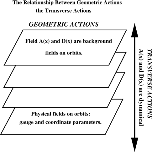
Figure 1: The Foliation of the Dual of the Algebra

This approach was applied to the isotropy equation obtained from the Virasoro algebra,

$$\delta_{\xi}D=2D^{\prime}\xi+D\xi^{\prime}+q\xi^{\prime\prime\prime}+\beta\xi^{\prime}=0$$ (63)

where

$$q={\textstyle{c\mu\over\vphantom{2}\smash{\raise 0.60275pt\hbox{$\scriptstyle{2\pi}$}}}}\ \ \ \ \mbox{and\ \ \ \ }\beta={\textstyle{h\mu\over\vphantom{2}\smash{\raise 0.60275pt\hbox{$\scriptstyle{2\pi}$}}}}.$$ (64)

Following the Yang-Mills case, we assume that this equation is obtained after enforcing the temporal gauge and on finds the transverse action,

$$S_{\mbox{\tiny diff}}= - \int d^{n}x\sqrt{g}~{}\alpha\left(X^{lmr}~{}{\rm D}^{a}{}_{r}X_{mla}+2X^{lmr}{\rm D}_{la}X^{a}{}_{rm}\right)$$

$$- \int d^{n}x\sqrt{g}\left(qX^{ab}{}_{b}{}\nabla_{l}\nabla_{m}{}X^{lm}{}_{a}+{\textstyle{\beta\over\vphantom{2}\smash{\raise 0.60275pt\hbox{$\scriptstyle{2}$}}}}X^{bga}X_{bga}-{\textstyle{1\over\vphantom{2}\smash{\raise 0.60275pt\hbox{$\scriptstyle{2}$}}}}X_{mnr}\left(x\right)X^{mnr}\left(x\right)\right)$$

where ${\rm X}^{mnr}=\nabla^{r}D^{mn}$. The term proportional to $q$ arises from the central extension in the algebra. Algebraically the central extension exists only in one dimension. However, in the construction of the transverse action, this contribution is seen as coming from a derivative interaction of the connection with the diffeomorphism field. We expect this term to be relevant in the early universe when there is only time dependence in the system. As we will see later, after time evolution, the $q$ dependence of the system becomes negligible. This could be the signature that the symmetries in the cosmological principle are broken and that spatial dependence becomes relevant.

A pictorial interpretation of the geometric and transverse action can be seen in Fig.(1). The geometric actions is the physics of the coordinates and gauge fields (collective coordinates) and is represented by horizontal slices on the foliation of the dual of the algebra. These horizontal slices are equivalence classes of fields and any physics there would constitute anomalies in the gauge and diffeomorphism symmetries. One the other hand, the transverse actions move the fields from one equivalence class to another and do not contain spurious gauge and coordinate degrees of freedom because of the Gauss law constraints. It is for this reason that we say that the transverse actions are transverse to the geometric actions. In $n$ dimensions the mass dimensions for the coupling constants and the diff field are:

$$\left[\alpha\right]={\textstyle{2-n\over\vphantom{2}\smash{\raise 0.60275pt\hbox{$\scriptstyle{2}$}}}},\ \ \ \left[\beta\right]=0,\ \ \ \left[q\right]=-2,\ {\mbox{\rm and}}\ \ \ \left[D_{\mu\nu}\right]={\textstyle{n-2\over\vphantom{2}\smash{\raise 0.60275pt\hbox{$\scriptstyle{2}$}}}}.$$ (66)

To see that the diffeomorphism action recovers Eq.(63) in two dimensions, we vary the action with respect to the space-time component ${\rm D}_{i0}$. Then by setting ${\rm D}_{i0}=0$, the field equation becomes

$$X^{lm0}\partial_{i}{\rm D}^{lm}-\partial_{m}(X^{ml0}{\rm D}_{li})-\partial_{l}(X^{ml0}{\rm D}_{mi})-q{~{}}\partial_{i}\partial_{l}\partial_{m}X^{lm0}=0.$$ (67)

In $1+1$ this corresponds to the isotropy equation found on the coadjoint orbit where D corresponds to to space-space component, $D_{11}$. The field equations in 1+1 dimensions reduce to

$$X{\rm D}^{\prime}+2X^{\prime}{\rm D}+q{~{}}X^{\prime\prime\prime}=0\,\,\rightarrow\,\,\xi{\rm D}^{\prime}+2\xi^{\prime}{\rm D}+q{~{}}\xi^{\prime\prime\prime}=0,$$ (68)

where the adjoint element $\xi$ corresponds to the conjugate momentum, $X\equiv X^{110}$, of ${\rm D}\equiv{\rm D}_{11}$. This action is exactly analogous to Yang-Mills theory.

4 Cosmology and the Diffeomorphism Field

We have seen that there are two types of physical action naturally arise from the coadjoint representations of the Virasoro algebras (diffeomorphisms) and Kac-Moody algebra (affine Lie algebra). One action is the geometric action that comes from the coadjoint orbits of algebras. The other action is from the phase space that is transverse to the coadjoint orbits: the transverse action. The transverse action of the Kac-Moody algebra is the Yang-Mills action in two dimensions and it is also valid in higher dimensions. The transverse action for the Virasoro algebra can be constructed by following the analogy of the construction for the Yang-Mills theory. The action associated with the algebra of diffeomorphisms is also valid in higher dimensions as its origins are Lie Derivatives.

The Virasoro algebra is the symmetry under coordinate transformation on the unit circle, i.e., diffeomorphisms. There an important lesson from string theory is that diffeomorphism should play an active role in the theory of gravitation. Indeed, we have already seen important implication of diffeomorphism in the geometric action for the Virasoro algebra Eq.[3.3]:

$${\textstyle{1\over\vphantom{2}\smash{\raise 0.60275pt\hbox{$\scriptstyle{2\pi}$}}}}\int d\tau d\theta D\left(\theta\right)\left({\textstyle{\partial_{\tau}s\over\vphantom{2}\smash{\raise 0.60275pt\hbox{$\scriptstyle{\partial_{\theta}s}$}}}}\right).$$ (69)

If we rewrite this term in coordinate invariant notion, we have

$$\int\sqrt{h}D_{ab}h^{ab}dx$$ (70)

where $h^{ab}$ is the inverse metric on the two manifold. Our interpretation of the diffeomorphism field $D$ is that it is a non-Riemannian contribution to gravitation: it appears already in two dimensions where the Einstein-Hilbert action only offers topological information. It is easy to observe that when the trace of $D_{ab}$ takes a constant value, this term appears as a natural source for the cosmological constant. Such a term in the action does not depend on the two dimensional structure.

In this section we will apply the transverse action of the Virasoro algebra to cosmology. More specifically, we will study the coupling of the trace part of the diffeomorphism field $D$ to the Robertson-Walker metric for the flat Universe ($k=1$) and study the cosmological implications of the diff field. Many of the calculations in this section are done by Mathematica with MathTensor package [References,References]. The action used to study the cosmological effect of the diff field $D$ has two parts:

$$S=S_{\mbox{\tiny HE}}+S_{\mbox{\tiny diff}}$$ (71)

where $S_{\mbox{\tiny HE}}$ is the Hilbert-Einstein action without cosmological constant and $S_{\mbox{\tiny diff}}$ is the transverse action for diff field:

$$S_{\mbox{\tiny HE}}=-{1\over 16\pi G}\int dx^{4}\sqrt{g\left(x\right)}R\left(x\right),\ \ \ \ \ x=\left(\vec{x},t\right)$$ (72)

and

$$S_{\mbox{\tiny diff}}= - \int d^{n}x\sqrt{g}~{}\alpha\left(X^{lmr}~{}{\rm D}^{a}{}_{r}X_{mla}+2X^{lmr}{\rm D}_{la}X^{a}{}_{rm}\right)$$

$$- \int d^{n}x\sqrt{g}\left(qX^{ab}{}_{b}{}\nabla_{l}\nabla_{m}{}X^{lm}{}_{a}+{\textstyle{\beta\over\vphantom{2}\smash{\raise 0.60275pt\hbox{$\scriptstyle{2}$}}}}X^{bga}X_{bga}\right)$$

$$- {\textstyle{1\over\vphantom{2}\smash{\raise 0.60275pt\hbox{$\scriptstyle{2}$}}}}\int d^{n}x\,\sqrt{g}X_{mnr}X^{mnr}+\lambda\int d^{n}x\sqrt{g}\,D_{\ m}^{m}.$$

We note that $\alpha$ term is from Gauss’ law constraint, $q$ and $\beta$ terms are from the central extension of the algebra. $\lambda$ term is analogous to Eq.70, i.e., the cosmological term. Since we will set the ordinary cosmological constant $\Lambda$ to zero, there will be no ambiguity. Again the mass dimensions in $n$ dimensions are

$$\left[\alpha\right]={\textstyle{2-n\over\vphantom{2}\smash{\raise 0.60275pt\hbox{$\scriptstyle{2}$}}}},\ \ \ \left[\beta\right]=0,\ \ \ \left[q\right]=-2,\ \ \ \left[\lambda\right]={\textstyle{n+2\over\vphantom{2}\smash{\raise 0.60275pt\hbox{$\scriptstyle{2}$}}}},\ \ \ \left[D_{\mu\nu}\right]={\textstyle{n-2\over\vphantom{2}\smash{\raise 0.60275pt\hbox{$\scriptstyle{2}$}}}}.$$ (74)

The equations of motion and the energy momentum tensor for the diff field $D_{\mu\nu}$ are obtained by varying the diff action $S_{\mbox{\tiny diff}}$ with respect to $D_{\mu\nu}$ and $g_{\mu\nu}$, respectively:

$$\mbox{equations of motion:\ \ \ }{\delta S_{\mbox{\tiny diff}}\over\delta D_{\mu\nu}}=0$$ (75)

and

$$\mbox{energy-momentum tensor:\ \ \ }\delta S_{\mbox{\tiny diff}}={\textstyle{1\over\vphantom{2}\smash{\raise 0.60275pt\hbox{$\scriptstyle{2}$}}}}\int d^{4}x\sqrt{g\left(x\right)}\,T^{\mu\nu}\left(x\right)\delta g_{\mu\nu}.$$ (76)

The trace of the diff field $D_{\mu\nu}$ is defined through the decomposition

$$D_{\mu\nu}\left(x\right)={\textstyle{1\over\vphantom{2}\smash{\raise 0.60275pt\hbox{$\scriptstyle{n}$}}}}\psi\left(x\right)g_{\mu\nu}+W_{\mu\nu}\left(x\right)$$ (77)

where $\psi\left(x\right)$ is a scalar field, $W_{\mu\nu}\left(x\right)$ is a traceless symmetric tensor field, and $n$ is the dimension of the spacetime. Since we are interested only in the trace part of the diff field $D_{\mu\nu}$, we set the traceless part to zero: $W_{\mu\nu}\left(x\right)=0$. The equations of motion for $D_{\mu\nu}\left(x\right)$, reduce to [References]

$$\left(4-{4\beta\over n}-2\alpha\left({2\over n^{2}}+{1\over n}\right)\psi\left(x\right)\right)\nabla^{\mu}\nabla_{\mu}\psi\left(x\right)$$ (78)

$$\ \ \ -\alpha\left({2\over n^{2}}+{1\over n}\right)\nabla^{\mu}\psi\left(x\right)\nabla_{\mu}\psi\left(x\right)-{1\over n}q\nabla^{\mu}\nabla^{\nu}\nabla_{\mu}\nabla_{\nu}\psi\left(x\right)+n\lambda=0.$$

where $\nabla_{\mu}$ is the covariant derivative. The energy-momentum tensor for $D_{\mu\nu}$ is reduced to [References]

$$T^{\mu\nu} = 2\left({2\over n}-{2\beta\over n^{2}}-\left({1\over n^{2}}+{2\over n^{3}}\right)\alpha\psi\left(x\right)\right)\nabla^{\mu}\psi\left(x\right)\nabla^{\nu}\psi\left(x\right)$$ (83)

$$+{q\over n^{2}}\left(\begin{array}[]{c}\nabla^{\sigma}\nabla_{\sigma}\psi\left(x\right)\nabla^{\mu}\nabla^{\nu}\psi\left(x\right)+\nabla_{\sigma}\psi\left(x\right)\nabla^{\sigma}\nabla^{\mu}\nabla^{\nu}\psi\left(x\right)\\ \\ -\nabla^{\mu}\psi\left(x\right)\nabla^{\sigma}\nabla^{\nu}\nabla_{\sigma}\psi\left(x\right)-\nabla^{\nu}\psi\left(x\right)\nabla^{\sigma}\nabla^{\mu}\nabla_{\sigma}\psi\left(x\right)\end{array}\right)$$

$$-\left({2\over n}-{2\beta\over n^{2}}-\left({1\over n^{2}}+{2\over n^{3}}\right)\alpha\psi\left(x\right)\right)\nabla^{\sigma}\psi\left(x\right)\nabla_{\sigma}\psi\left(x\right)g^{\mu\nu}$$

$$-{q\over 2n^{2}}\nabla^{\sigma}\nabla^{\tau}\psi\left(x\right)\nabla_{\sigma}\nabla_{\tau}\psi\left(x\right)g^{\mu\nu}$$

$$+\lambda\psi\left(x\right)g^{\mu\nu}.$$

Applying the cosmological principle to the diffeomorphism field, we write, in four dimensions,

$$D_{\mu\nu}\left(t\right)={\textstyle{1\over\vphantom{2}\smash{\raise 0.60275pt\hbox{$\scriptstyle{4}$}}}}f(t)g_{\mu\nu}$$ (84)

where $f(t)=\psi\left(\vec{x},t\right)$ is a scalar function that only depends on time. Using this form of diff field, we find the equation of motion for the diff field as

$$\begin{array}[]{c}\left(1-{\textstyle{\beta\over\vphantom{2}\smash{\raise 0.60275pt\hbox{$\scriptstyle{4}$}}}}-{\textstyle{3\over\vphantom{2}\smash{\raise 0.60275pt\hbox{$\scriptstyle{16}$}}}}\alpha f\left(t\right)\right)f^{\prime\prime}\left(t\right)+3H\left[\left(1-{\textstyle{\beta\over\vphantom{2}\smash{\raise 0.60275pt\hbox{$\scriptstyle{4}$}}}}-{\textstyle{3\over\vphantom{2}\smash{\raise 0.60275pt\hbox{$\scriptstyle{16}$}}}}\alpha f\left(t\right)\right)f^{\prime}\left(t\right)+{\textstyle{1\over\vphantom{2}\smash{\raise 0.60275pt\hbox{$\scriptstyle{16}$}}}}qf^{\left(3\right)}\left(t\right)\right]\\ \\ +\lambda-{\textstyle{3\over\vphantom{2}\smash{\raise 0.60275pt\hbox{$\scriptstyle{32}$}}}}\alpha f^{\prime}(t)^{2}+{\textstyle{1\over\vphantom{2}\smash{\raise 0.60275pt\hbox{$\scriptstyle{16}$}}}}qf^{\left(4\right)}(t)+{\textstyle{3\over\vphantom{2}\smash{\raise 0.60275pt\hbox{$\scriptstyle{8}$}}}}qH^{2}f^{{}^{\prime\prime}}f\\ \\ -{\textstyle{9\over\vphantom{2}\smash{\raise 0.60275pt\hbox{$\scriptstyle{16}$}}}}qH^{3}f^{\prime}(t)+{\textstyle{3\over\vphantom{2}\smash{\raise 0.60275pt\hbox{$\scriptstyle{16}$}}}}qH^{\prime}f^{\prime\prime}(t)-{\textstyle{3\over\vphantom{2}\smash{\raise 0.60275pt\hbox{$\scriptstyle{8}$}}}}qf^{\prime}(t)H^{\prime}H=0\end{array}$$ (85)

Here we used ‘ ^′ ’ as a time derivative and $H=H\left(t\right)$. The energy density and pressure of the diff field are also found, respectively, as

$$\rho_{\mbox{\tiny diff}}\left(t\right) = {\textstyle{1\over\vphantom{2}\smash{\raise 0.60275pt\hbox{$\scriptstyle{2}$}}}}\left(1-{\textstyle{\beta\over\vphantom{2}\smash{\raise 0.60275pt\hbox{$\scriptstyle{4}$}}}}-{\textstyle{3\over\vphantom{2}\smash{\raise 0.60275pt\hbox{$\scriptstyle{16}$}}}}\alpha f\left(t\right)\right)f^{\prime}\left(t\right)^{2}+\lambda f\left(t\right)$$

$$+{\textstyle{7\over\vphantom{2}\smash{\raise 0.60275pt\hbox{$\scriptstyle{32}$}}}}qH^{2}f^{\prime}\left(t\right)^{2}+{\textstyle{1\over\vphantom{2}\smash{\raise 0.60275pt\hbox{$\scriptstyle{8}$}}}}qHf^{\prime}\left(t\right)f^{\prime\prime}\left(t\right)-{\textstyle{1\over\vphantom{2}\smash{\raise 0.60275pt\hbox{$\scriptstyle{32}$}}}}qf^{{}^{\prime\prime}}\left(t\right)^{2}$$

and

$$p_{\mbox{\tiny diff}}\left(t\right) = {\textstyle{1\over\vphantom{2}\smash{\raise 0.60275pt\hbox{$\scriptstyle{2}$}}}}\left(1-{\textstyle{\beta\over\vphantom{2}\smash{\raise 0.60275pt\hbox{$\scriptstyle{4}$}}}}-{\textstyle{3\over\vphantom{2}\smash{\raise 0.60275pt\hbox{$\scriptstyle{16}$}}}}\alpha f\left(t\right)\right)f^{\prime}\left(t\right)^{2}-\lambda f\left(t\right)$$

$$- {\textstyle{9\over\vphantom{2}\smash{\raise 0.60275pt\hbox{$\scriptstyle{32}$}}}}qH^{2}f^{\prime}\left(t\right)^{2}+{\textstyle{3\over\vphantom{2}\smash{\raise 0.60275pt\hbox{$\scriptstyle{16}$}}}}qHf^{\prime}\left(t\right)f^{\prime\prime}\left(t\right)-{\textstyle{1\over\vphantom{2}\smash{\raise 0.60275pt\hbox{$\scriptstyle{32}$}}}}qf^{{}^{\prime\prime}}\left(t\right)^{2}+{\textstyle{1\over\vphantom{2}\smash{\raise 0.60275pt\hbox{$\scriptstyle{16}$}}}}qf^{\prime}\left(t\right)f^{\left(3\right)}\left(t\right).$$

Note that the equation of motion for the diff field depends on both $H$ and $H^{\prime}$, where as the energy density and the pressure only depend on $H$. The equation of state, the pressure-to-energy density ratio, $w\left(t\right)$, for the diff field is given by

$$w\left(t\right)={p_{\mbox{\tiny diff}}\left(t\right)\over\rho_{\mbox{\tiny diff}}\left(t\right)}$$ (88)

To study the properties of the diff field in the early universe, we assume that the contributions from the other sources are negligible. In other words, we set the energy densities and pressures for other matters (including radiation) to zero. Under this assumption the Friedmann equations can be written in terms of the scalar field $f\left(t\right)$ and its derivatives in time:

$$H^{2}(t) = {1\over 3M_{\rm pl}^{2}}\left[\begin{array}[]{c}{\textstyle{1\over\vphantom{2}\smash{\raise 0.60275pt\hbox{$\scriptstyle{2}$}}}}\left(1-{\textstyle{\beta\over\vphantom{2}\smash{\raise 0.60275pt\hbox{$\scriptstyle{4}$}}}}-{\textstyle{3\over\vphantom{2}\smash{\raise 0.60275pt\hbox{$\scriptstyle{16}$}}}}\alpha f\left(t\right)\right)f^{\prime}\left(t\right)^{2}+\lambda f\left(t\right)\\ \\ +{\textstyle{7\over\vphantom{2}\smash{\raise 0.60275pt\hbox{$\scriptstyle{32}$}}}}qH^{2}f^{\prime\prime}\left(t\right)+{\textstyle{1\over\vphantom{2}\smash{\raise 0.60275pt\hbox{$\scriptstyle{8}$}}}}qHf^{\prime}\left(t\right)f^{\prime\prime}\left(t\right)-{\textstyle{1\over\vphantom{2}\smash{\raise 0.60275pt\hbox{$\scriptstyle{32}$}}}}qf^{{}^{\prime\prime}}\left(t\right)^{2}\end{array}\right]$$ (92)

$$H^{\prime}\left(t\right) = -{1\over 2M_{\mbox{p}l}^{2}}\left[\begin{array}[]{c}\left(1-{\textstyle{\beta\over\vphantom{2}\smash{\raise 0.60275pt\hbox{$\scriptstyle{4}$}}}}-{\textstyle{3\over\vphantom{2}\smash{\raise 0.60275pt\hbox{$\scriptstyle{16}$}}}}\alpha f\left(t\right)\right)f^{\prime}\left(t\right)^{2}\\ \\ -{1\over 16}qf^{{}^{\prime\prime}}\left(t\right)^{2}+{\textstyle{1\over\vphantom{2}\smash{\raise 0.60275pt\hbox{$\scriptstyle{16}$}}}}qf^{\prime}\left(t\right)f^{\left(3\right)}\left(t\right)\\ \\ -{\textstyle{1\over\vphantom{2}\smash{\raise 0.60275pt\hbox{$\scriptstyle{16}$}}}}qH^{2}f^{\prime}\left(t\right)^{2}+{\textstyle{5\over\vphantom{2}\smash{\raise 0.60275pt\hbox{$\scriptstyle{16}$}}}}qHf^{\prime}\left(t\right)f^{\prime\prime}\left(t\right)\end{array}\right]$$ (98)

The expression of Hubble parameter $H\left(t\right)$ can be obtained from Eq.92. Since it is in a quadratic form in $H$, we have two possibilities:

$$H_{\pm}(t)={1\over 96M_{\mbox{p}l}^{2}+9qf^{\prime}\left(t\right)^{2}}\left[3qf^{\prime}\left(t\right)f^{\prime\prime}\left(t\right)\pm\sqrt{Q}\right]$$ (99)

where

$$Q = 9q^{2}f^{\prime}\left(t\right)^{2}f^{\prime\prime}\left(t\right)^{2}$$ (103)

$$-\left(96M_{pl}^{2}+9qf^{\prime}\left(t\right)^{2}\right)\left(\begin{array}[]{c}4\left(\beta-4\right)f^{\prime}\left(t\right)^{2}+f\left(t\right)\left(32\lambda+3\alpha f^{\prime}\left(t\right)^{2}\right)\\ +qf^{\prime\prime}\left(t\right)^{2}-2qf^{\prime}\left(t\right)f^{\left(3\right)}\left(t\right)\end{array}\right).$$

The Friedmann equations, Eq.92 and Eq.98, also allow us to simplify the equation of motion for $D_{\mu\nu}$, Eq.85: these two equations can be used to eliminate $H$ and $H^{\prime}$ in the equation of motion for $D_{\mu\nu}$.

5 Numerical Results

We will numerically solve the equation of motion for the trace part of $D_{\mu\nu}$ in the Robertson-Walker metric. We use the numerical solution of $f\left(t\right)$ to plot the Hubble parameter $H\left(t\right)$, energy-density $\rho\left(t\right)$, pressure $p\left(t\right)$, the equation of state $w\left(t\right)$ and $\rho\left(t\right)+3p\left(t\right)$. Since the equation of motion that we are studying is very complicated, we will limit our analysis to the basic behavior of each quantities under given set of parameters and initial conditions. Our main goal in this numerical computation is not to obtain the results that agree with the current observation, but to investigate the effects of the trace part of diff field $D_{\mu\nu}$ on the quantities mentioned above to study the nature of the scalar field $f\left(t\right)$. We use the explicit Runge-Kutta method for this numerical computation.

5.1 Parameters

Eq.99 suggests that the Hubble parameter $H\left(t\right)$ is expected to increase its magnitude very rapidly as

$$f^{\prime}\left(t\right)^{2}\rightarrow-{\textstyle{32\over\vphantom{2}\smash{\raise 0.60275pt\hbox{$\scriptstyle{3q}$}}}}M_{\mbox{p}l}^{2}.$$ (104)

The above condition also implies that the value of $q$ should be negative. In this limit it is not difficult see that the positive solution (the solution with $+\sqrt{Q}$) has a simpler behavior near the “peak”. Hence, in the following, we will study the positive solution case. Noting that the function of parameter $\beta$ is basically to shift the value of kinetic term, we set this parameter to zero. Noting that the mass dimension scalar field $f\left(t\right)$ is one, so it’s natural to use the planck mass $M_{pl}$ for this scalar field, i.e., we set $M_{pl}$ to one. Hence undetermined parameters are $\alpha$, $q$, and $\lambda$.

5.2 Trial Initial Conditions

The equation of motion for the trace part of $D_{\mu\nu}$ in the Robertson-Walker metric is a fourth order nonlinear differential equation with three parameters (after setting $\beta=0$ and $M_{pl}=1$). To solve these differential equations numerically, we need to specify trial values for the three parameters and four initial conditions. In this numerical computation the initial conditions for $f\left(t\right)$, $f^{\prime}\left(t\right)$, $f^{\prime\prime}\left(t\right)$, and $f^{\left(3\right)}\left(t\right)$ are used. A priori, we do not know how to choose these parameters and initial conditions. To overcome this, we use the physical condition on the Hubble parameter as a guide for choosing the trial values. We search for a set of the parameters and the initial conditions that give a positive and finite value for the Hubble parameter. With this as a criterion, a choice for the trial of parameters and the initial conditions become

$$\alpha=-1,\ \ \ q=-6,\ \ \ \lambda=0.05,$$

$$f\left(0\right) = -10,\ f^{\prime}\left(0\right)=0,\ f^{\prime\prime}(0)=-1,\ f^{\left(3\right)}=-1.$$ (105)

This set of trial values give the Hubble parameter plot shown in Fig.2.

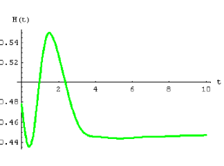
Figure 2: The Trial Hubble Parameter Plot

Note that we used$\ k=0$ (flat Universe), $\Lambda=0$ (no cosmological constant), $\beta=0$, and $M_{\mbox{p}l}=1$.

5.3 Computation

As we have noted in Chapter 1, the nature of scalar fields are characterized by the equation of state $w\left(t\right)$, and this value is defined as the ratio of the pressure $p\left(t\right)$ to the energy density $\rho\left(t\right)$. The acceleration of Universe can be studied through the quantity $\rho\left(t\right)+3p\left(t\right)$. We, thus, compute $f\left(t\right)$, $H\left(t\right)$, $\rho\left(t\right)$, $p\left(t\right)$, $w\left(t\right)$, and $\rho\left(t\right)+3p\left(t\right)$ for the reference set and study the effect of variations in two parameters ($q$ and $\lambda$) and four initial conditions of the scalar field $f\left(t\right)$ ($f\left(0\right)$, $f^{\prime}\left(0\right)$, $f^{\prime\prime}\left(0\right)$, and $f^{\left(3\right)}\left(0\right)$) on these quantities. The following is the sets of two parameters ($q$ and $\lambda$) and four initial conditions of the scalar field $f\left(t\right)$ ($f\left(0\right)$, $f^{\prime}\left(0\right)$, $f^{\prime\prime}\left(0\right)$, and $f^{\left(3\right)}\left(0\right)$) used in this numerical computation

5.4 Results

The effect of changes in two parameters ($q$ and $\lambda$) and four initial conditions on the scalar field $f\left(t\right)$ ($f\left(0\right)$, $f^{\prime}\left(0\right)$, $f^{\prime\prime}\left(0\right)$, and $f^{\left(3\right)}\left(0\right)$) are studied. Each parameter/initial condition is varied with respect to the corresponding starting value. The results are plotted for the scalar field $f\left(t\right)$, Hubble parameter $H\left(t\right)$, energy density $\rho\left(t\right)$, pressure $P\left(t\right)$, and the equation of state (pressure-to-energy density ratio) $w\left(t\right)$. The unspecified values are the same as that of the reference set Eq 105. Here are our results.

5.5 Effect of Changes in $q$

Red $(\cdots)$   $q=-2$ , Green $(^{\underline{\,\,\,\,\,\,\,}})$ $q=-6$ ,  Blue (- -) $q=-8$

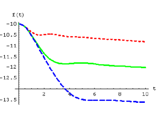
Figure 3: Scalar field $f(t)$ obtained with $q=-2$ (red), $-6$ (green), $-8$ (blue)

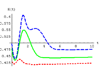
Figure 4: Hubble parameter $H(t)$ obtained with $q=-2$ (red), $-6$ (green), $-8$ (blue)

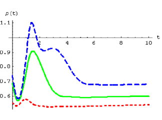
Figure 5: Energy density $\rho(t)$ with $q=-2$ (red), $-6$ (green), $-8$ (blue)

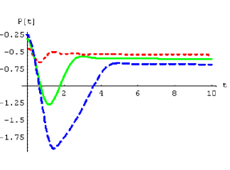
Figure 6: Pressure $p(t)$ obtained with $q=-2$ (red), $-6$ (green), $-8$ (blue)

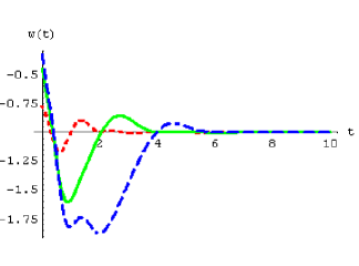
Figure 7: Equation of State $w(t)$ obtained with $q=-2$ (red), $-6$ (green), $-8$ (blue)

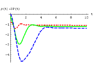
Figure 8: $\rho(t)+3p(t)$ obtained with $q=-2$ (red), $-6$ (green), $-8$ (blue)

5.6 Effect of Change in $\lambda$

Red $(\cdots)$   $\lambda=0.08$ , Green $(^{\underline{\,\,\,\,\,\,\,}})$ $\lambda=0.05$ ,  Blue (- -) $\lambda=0.02$

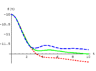
Figure 9: $f(t)$ obtained with $\lambda=0.08$ (red), $0.05$ (green), $0.02$ (blue)

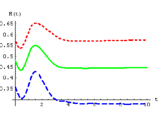
Figure 10: $H(t)$ obtained with $\lambda=0.08$ (red), $0.05$ (green), $0.02$ (blue)

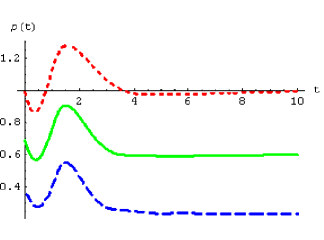
Figure 11: $\rho(t)$ obtained with $\lambda=0.08$ (red), $0.05$ (green), $0.02$ (blue)

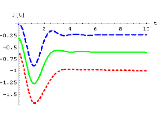
Figure 12: $p(t)$ obtained with $\lambda=0.08$ (red), $0.05$ (green), $0.02$ (blue)

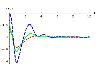
Figure 13: Equation of State $w(t)$ obtained with $\lambda=0.08$ (red), $0.05$ (green), $0.02$ (blue)

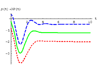
Figure 14: $\rho(t)+3p(t)$ obtained with $\lambda=0.08$ (red), $0.05$ (green), $0.02$ (blue)

5.7 Effect of Change in Initial Value of $f\left(t_{0}\right)$

Red $(\cdots)$   $f(t_{0})=-8$ , Green $(^{\underline{\,\,\,\,\,\,\,}})$ $f(t_{0})=-10$ ,  Blue (- -) $f(t_{0})=-12$

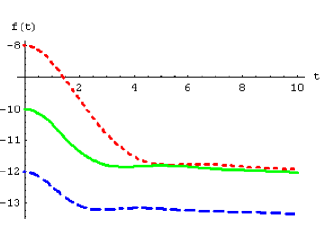
Figure 15: Scalar field $f(t)$ obtained with $f(t_{0})=-8$ (red), $-10$ (green), $-12$ (blue)

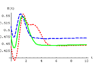
Figure 16: Hubble parameter $H(t)$ obtained with $f(t_{0})=-8$ (red), $-10$ (green), $-12$ (blue)

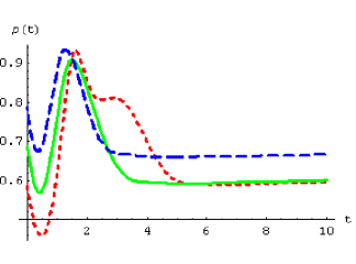
Figure 17: Energy Density $\rho(t)$ obtained with $f(t_{0})=-8$ (red), $-10$ (green), $-12$ (blue)

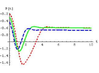
Figure 18: Pressure $p(t)$ obtained with $f(t_{0})=-8$ (red), $-10$ (green), $-12$ (blue)

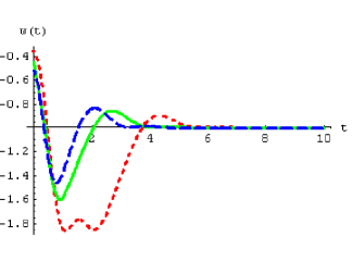
Figure 19: Equation of State $w(t)$ obtained with $f(t_{0})=-8$ (red), $-10$ (green), $-12$ (blue)

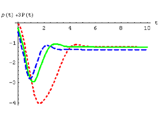
Figure 20: $\rho(t)+3p(t)$ obtained with $f(t_{0})=-8$ (red), $-10$ (green), $-12$ (blue)

5.8 Effect of Change in Initial Value of $f^{\prime}\left(t_{0}\right)$

Red $(\cdots)$   $f^{\prime}\left(t_{0}\right)=-0.5$ , Green $(^{\underline{\,\,\,\,\,\,\,}})$ $f^{\prime}\left(t_{0}\right)=0$ ,  Blue (- -) $f^{\prime}\left(t_{0}\right)=0.5$

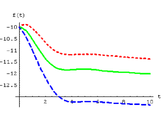
Figure 21: Scalar field $f(t)$ obtained with $f^{\prime}(t_{0})=-0.52$ (red), $0$ (green), $0.5$ (blue)

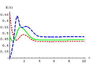
Figure 22: Scalar field $H(t)$ obtained with $f^{\prime}(t_{0})=-0.52$ (red), $0$ (green), $0.5$ (blue)

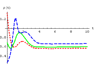
Figure 23: Energy density $\rho(t)$ obtained with $f^{\prime}(t_{0})=-0.52$ (red), $0$ (green), $0.5$ (blue)

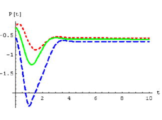
Figure 24: Pressure $p(t)$ obtained with $f^{\prime}(t_{0})=-0.52$ (red), $0$ (green), $0.5$ (blue)

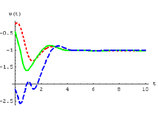
Figure 25: Equation of state $w(t)$ obtained with $f^{\prime}(t_{0})=-0.52$ (red), $0$ (green), $0.5$ (blue)

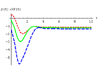
Figure 26: $\rho(t)+3p(t)$ obtained with $f^{\prime}(t_{0})=-0.52$ (red), $0$ (green), $0.5$ (blue)

5.9 Effect of Change in Initial Value of $f^{\prime\prime}\left(t_{0}\right)$

Red $(\cdots)$   $f^{\prime\prime}(t_{0})=-0.5$ , Green $(^{\underline{\,\,\,\,\,\,\,}})$ $f^{\prime\prime}(t_{0})=-1$ ,  Blue (- -) $f^{\prime\prime}(t_{0})=-1.5$

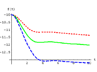
Figure 27: Scalar field $f(t)$ with $f^{\prime\prime}(t_{0})=-8$ (red), $-10$ (green), $-12$ (blue)

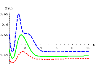
Figure 28: Hubble parameter $H(t)$ with $f^{\prime\prime}(t_{0})=-8$ (red), $-10$ (green), $-12$ (blue)

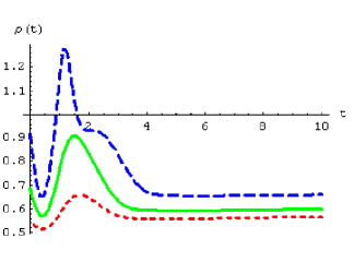
Figure 29: Energy density $\rho(t)$ with $f^{\prime\prime}(t_{0})=-8$ (red), $-10$ (green), $-12$ (blue)

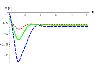
Figure 30: Pressure $p(t)$ with $f^{\prime\prime}(t_{0})=-8$ (red), $-10$ (green), $-12$ (blue)

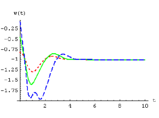
Figure 31: Equation of state $w(t)$ with $f^{\prime\prime}(t_{0})=-8$ (red), $-10$ (green), $-12$ (blue)

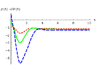
Figure 32: $\rho(t)+3p(t)$ with $f^{\prime\prime}(t_{0})=-8$ (red), $-10$ (green), $-12$ (blue)

5.10 Effect of Change in Initial Value of $f^{\left(3\right)}\left(t_{0}\right)$

Red $(\cdots)$   $f^{\left(3\right)}=-0.5$ , Green $(^{\underline{\,\,\,\,\,\,\,}})$ $f^{\left(3\right)}=-1$ ,  Blue (- -) $f^{\left(3\right)}=-1.5$

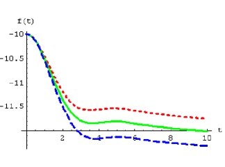
Figure 33: Scalar field $f(t)$ obtained with $f^{(3)}(t_{0})=-0.5$ (red), $-1$ (green), $-1.5$ (blue)

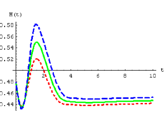
Figure 34: Hubble parameter $H(t)$ obtained with $f^{(3)}(t_{0})=-0.5$ (red), $-1$ (green), $-1.5$ (blue)

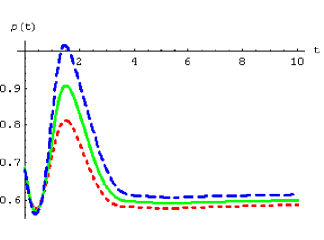
Figure 35: Energy density $\rho(t)$ obtained with $f^{(3)}(t_{0})=-0.5$ (red), $-1$ (green), $-1.5$ (blue)

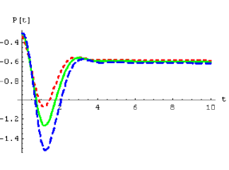
Figure 36: Pressure $p(t)$ obtained with $f^{(3)}(t_{0})=-0.5$ (red), $-1$ (green), $-1.5$ (blue)

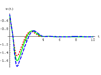
Figure 37: Equation of state $w(t)$ obtained with $f^{(3)}(t_{0})=-0.5$ (red), $-1$ (green), $-1.5$ (blue)

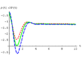
Figure 38: $\rho(t)+3p(t)$ obtained with $f^{(3)}(t_{0})=-0.5$ (red), $-1$ (green), $-1.5$ (blue)

6 Conclusion

From the plots obtained in the last section we find that the equation of state $w\left(t\right)$ can take, at least, values between $-2$ and $0$. Most interestingly it always converges to $-1$ after some time for all the initial conditions we used. It means that the trace part of the diff field $D_{\mu\nu}$ acts like a cosmological constant $\Lambda$ in later times. This scalar field spends most of the time before $w=-1$ as a phantom dark energy. This is a time-dependent phantom dark energy and its effects on Universe will be different from the time-independent cases [References, References, References]. Since the equation of state $w$ can be $0$ in the very early Universe, it behaves as a dark matter when it happens. The fact that the value of $w$ never gets close to $1/3$ is very desirable because otherwise the radiation-like behavior of the scalar field at early times would influence already well explained primordial nucleosynthesis [References].

The effects on the scalar field on the Hubble parameter are also notable. It is easy to see that there are expected peaks [Eq.99]. Figure 4, Figure 16, Figure 22, and Figure 28 show shoulder-like regions where the value of Hubble parameter stay almost constant, i.e., the universe is expanding exponentially over this region:

$$H={\textstyle{\dot{a}\over\vphantom{2}\smash{\raise 0.60275pt\hbox{$\scriptstyle{a}$}}}}={\mbox{constant}}\rightarrow a\left(t\right)\sim e^{Ht}.$$ (106)

This scalar field, hence, acts like an inflaton over these regions. The constant Hubble parameter in later time can be interpreted as the current expansion of the Universe due to the cosmological constant like behavior of the scalar field. The last important observation is that the value of $\rho\left(t\right)+3p\left(t\right)$ is almost always negative. That is, this scalar contributes to the acceleration of Universe for most of time.

Though our results are qualitative, they are showing very interesting cosmological implications of the diffeomorphism field $D_{\mu\nu}$: the trace part of the diffeomorphism field $D_{\mu\nu}$ can produce the inflation-like behavior of the Universe in early time and the accelerating Universe in later time qualitatively. It is also observed that the time-dependent phantom dark energy plays a crucial role in this model. Our results, however, lack the realistic prediction: $e$-foldings $N$,

$$N\left(t\right)=\ln{\textstyle{a\left(t_{\mbox{\tiny end}}\right)\over\vphantom{2}\smash{\raise 0.60275pt\hbox{$\scriptstyle{a\left(t\right)}$}}}}=\int_{t}^{t_{end}}H\left(t\right)dt,$$ (107)

during “inflation” predicted by this model is about $N\sim 2$, whereas any realistic model for inflation requires $N\sim 70$. This suggest that more research in the study the set of parameters and the initial values necessary to make sensible predictions. Furthermore the understanding of the time-dependent phantom dark energy is essential in future research.

References

- [1] C, Armendariz-Picón, T. Damour, V. Mukhanov, hep-th/9904075 v1
- [2] C, Armendariz-Picón and V. Mukhanov, Phys. Rev. D 63, 103510 (2001)
- [3] C, Armendariz-Picón, V. Mukhanov, and P.J. Steinhardt, Phys. Rev. Lett. 85, 4438 (2000)
- [4] A. Alekseev and S. Shatashvili, Nucl. Phys. B323 719 (1989)
- [5] V.I. Arnold, Mathematical Methods of Classical Mechanics, 2nd. ed. Springer-Verlag, (1989)
- [6] T.Branson, R.P. Lano and V.G.J. Rodgers, Phys. Lett. B 412, 253 (1997)
- [7] V. Barger, J.P. Kneller, H.-S. Lee, D. Marfatia, and G. Steigman, Phys. Lett B 566, 8 (2003)
- [8] T.P. Branson, V.G.J. Rodgers, T. Yasuda, Int. J. Mod. Phys. A Vol. 15, 3549 (2000)
- [9] R.R. Caldwell, Brazilian Journal of Physics, vol 30, no 2 215
- [10] R.R. Caldwell, astro-ph/9908168 v2
- [11] R. -G. Cai and A. Wnag, hep-th/0411025
- [12] S. Dodelson, Modern Cosmology, Academic Press (2003)
- [13] G.W. Delius, P. van Nieuwenhuizen and V.G.J. Rodgers, Int. J. Mod. Phys. A5 3943 (1990)
- [14] A. Gruzinov, astro-ph/0405096 v1
- [15] A. A. Kirillov, Unitary representations of nilpotent Lie groups, Uspekhi Mat. Nauk 17 (1962)
- [16] A. A. Kirillov, Elements of the Theory of Reperesentations, Springer-Verlag (1975)
- [17] A.A. Kirillov, Lect. Notes in Math. 970 101, Springer-Verlag (Berlin, 1982)
- [18] A. A. Kirillov, Lectures on the Orbit Method, AMS (2000)
- [19] V.G. Kac and A.K. Raina, Bombay Lectures on Highest Weight Representaions of infinite Dimensional Lie Algebras World Scientific Publishing (1987)
- [20] R.P. Lano and V.G.J. Rodgers, Nucl. Phys. B437 (1995) 45
- [21] R.P. Lano and V.G.J. Rodgers, Mod. Phys. Lett. A7 (1992) 1725
- [22] A.M. Polyakov, Mod. phys. Lett. A2 No.11 (1987) 893
- [23] L. Parker and S.M. Christensen, MathTensor, Addison-Wesley Publishing Company (1994)
- [24] P.J. Peebles, Principles of Physical Cosmology, Princeton University Press (Princeton, 1993)
- [25] A. Pressley and G Segal, Loop Groups, Oxford Univ. Press (Oxford,1986)
- [26] B. Rai and V.G.J. Rodgers, Nucl. Phys. B341 (1990) 119
- [27] V.G.J. Rodgers, T. Yasuda, Mod.Phys.Lett. A18, 2467 (2003)
- [28] R.J. Scherrer, astro-ph/0402316v3
- [29] http://panisse.lbl.gov/public/
- [30] M.A. Virasoro, Phys. Rev. Lett. 22 (1969) 37
- [31] P.B. Wiegmann, Nucl. Phys. B323 (1989) 311
- [32] R.M. Wald, General Relativity, The University of Chicago Press (1984)
- [33] S. Weinberg, Gravitation and Cosmology, John Wiley & Sons, Inc. (1972)
- [34] E. Witten, Comm. Math. Phys. 92 (1984) 455
- [35] E. Witten, Comm. Math. Phys. 114 (1988) 1
- [36] http//lambda.gsfc.nasa.gov/
- [37] S. Wolfram, The MATHEMATICA Book, Version 3, Cambridge University Press (1996)
- [38] Takeshi Yasuda, The Cosmological Implications of Diffeomorphsims Ph.D. thesis, The University of Iowa (2006)