High-energy effects on the spectrum of inflationary gravitational wave background in braneworld cosmology

Abstract

We discuss the cosmological evolution of the inflationary gravitational wave background (IGWB) in the Randall-Sundrum single-brane model. In braneworld cosmology, in which three-dimensional space-like hypersurface that we live in is embedded in five-dimensional anti de Sitter (AdS₅) spacetime, the evolution of gravitational wave (GW) modes is affected by the non-standard expansion of the universe and the excitation of the Kaluza-Klein modes (KK-modes). These are significant in the high-energy regime of the universe. We numerically evaluate these two effects by solving the evolution equation for GWs propagating through the AdS₅ spacetime. Using a plausible initial condition from inflation, we find that the excitation of KK-modes can be characterized by a simple scaling relation above the critical frequency $f_{\rm crit}$ determined from the length scale of the fifth dimension $\ell$. The remarkable point is that this relation generally holds as long as the matter content of the universe is described by the perfect fluid with the equation of state (EOS) $p=w\rho$ for $0\leq w\leq 1$. The resultant scaling relation is translated into the energy spectrum of the IGWB as $\Omega_{\rm GW}\propto f^{(3w-1)/(3w+2)}$ for $f>f_{\rm crit}$. This indicates that in the radiation dominant case ($w=1/3$), the two high-energy effects accidentally compensate each other and the spectrum becomes almost the same as the one predicted in the four-dimensional theory, i.e., $\Omega_{\rm GW}\propto f^{0}$.

I Introduction

Gravitational waves (GWs) are ultimate probes of the untouched region of the universe. Currently, large scale ground-based interferometers (TAMA300Ando and the TAMA Collaboration (2005), LIGOSigg (2004), VIRGOAcernese et al. (2005), GEO600Grote et al. (2005)) are enthusiastically trying to detect the signals emitted from stellar objects with relativistic motion – supernovae explosions, coalescence of neutron star binaries and so on. Among numerous types of GWs, the gravitational wave background (GWB) may possess much interesting information on the cosmology, though its detection is expected to be so challenging Abbott et al. (2005). Especially, the inflationary GWB (IGWB), generated during the inflationary epoch by the quantum fluctuations of the spacetimeStarobinskii (1979); Rubakov et al. (1982); Fabbri and Pollock (1983); Abbott and Wise (1984a, b); Abbott and Harari (1986); Allen (1988); Turner (1997); Maggiore (2000), is thought to be one of the most fundamental predictions of the inflationary scenario Sato (1981); Guth (1981); Linde (1982); Albrecht and Steinhardt (1982). Since the history of the cosmological expansion is imprinted in the power spectrum of the IGWB, it helps us to understand the extremely early universe if we can detect the signals by the future space-based experiments, such as DECIGOSeto et al. (2001) and BBOBBO ; Ungarelli et al. (2005).

As an ultimate cosmological tool, the IGWB may also be useful to probe the presence of extra-dimensional spaces. Recent developments in particle physics suggest that we live in a higher dimensional spacetime. In particular, braneworld scenarios have recently attracted much attention theoretically and observationally (for a review, see Maartens (2004)). According to them, we live in a three-dimensional hypersurface (brane) embedded in the higher-dimensional spacetime (bulk). While gravity can propagate in the bulk with the curvature scale $\ell$, the standard model particles are confined to the three-dimensional brane. In the low-energy regime of the universe ($H\ell\ll 1$), four-dimensional general relativity is successfully recovered and the extra-dimensional effects should be fairly small. On the other hand, in the high-energy regime ($H\ell\gg 1$), the localization of gravity is not always guaranteed and a significant deviation of the time evolution of GWs from the standard four-dimensional theory is expected. If this scenario is true, the spectrum of the IGWB may be significantly modified by the high-energy effects, which can provide a direct probe of the extra-dimensions.

The goal of this paper is to investigate the high-energy effects on the evolution of the IGWB and quantify the power spectrum. During the inflationary epoch, the wavelength of the GWs exceeds the Hubble horizon scale due to the exponential expansion of the universe and the amplitude of GWs becomes frozen. After the end of inflation, the universe enters the decelerated expansion phase and wavelengths of GWs soon become shorter than the Hubble scale. When the Hubble horizon scale becomes comparable or smaller than the characteristic size of the extra-dimension, the high-energy effects may significantly affect the evolution of GWs. There are two main high-energy effects : i) peculiar cosmological expansion due to the high-energy correction of the Friedmann equation, which enhances the spectrum in the high frequency region and ii) excitation of Kaluza-Klein modes (KK-modes) freely escaping from the brane to the bulk spacetime, which may suppress the amplitude of the GWs on the brane. While the former effect is simply estimated from the expansion rate of the universe, the amount of the latter effect requires the knowledge of the wave propagation in the bulk. Focusing on the Randall-Sundrum single-brane model, in which the three-dimensional hypersurface (brane) is embedded in the five-dimensional anti-de Sitter (AdS₅) spacetimeRandall and Sundrum (1999), many authors have tried to estimate these effects in an analytic way. However, these analyses were restricted to the idealistic situations Gorbunov et al. (2001); Kobayashi et al. (2003); Kobayashi and Tanaka (2004) or low-energy cases in the Friedmann universe Battye et al. (2003); Easther et al. (2003), since the analytic study of wave equation is generally intractable due to the complicated form of equation as well as boundary condition. Thus, in this paper, we numerically solve the wave equation and try to estimate the observed IGWB spectrum.

Concerning numerical studies, several authors have used different numerical techniques and coordinate systems to solve the wave equation of GWs Hiramatsu et al. (2004, 2005); Ichiki and Nakamura (2003); Kobayashi and Tanaka (2005a, b); Seahra (2006). In our previous studies Hiramatsu et al. (2004, 2005), numerical simulations were carried out in the two types of coordinate systems. One is the Gaussian normal coordinate system in which we found the suppression of the amplitude of the IGWB on the brane. Unfortunately, the coordinate singularity appears in the bulk and this restricts our analyses to a relatively low-energy scale Hiramatsu et al. (2004). On the other hand, another coordinate system we used is the Poincaré coordinates in which we observed that the two high-energy effects compensate each other and the spectrum became same one as predicted in the four-dimensional theory Hiramatsu et al. (2005).

In this paper, we first show that the spectrum of the IGWB estimated in the paper Hiramatsu et al. (2005) is robust against several numerical artifacts, such as the dependence of the regulator brane and initial time. Next, we study the dependence of the spectra on the equation of state (EOS) of the universe to clarify how the two high-energy effects change with the expansion rate of the universe.

This paper consists of seven sections. In Sec. 2, we discuss how the spectrum of the IGWB is affected by the presence of the extra-dimensions. In Sec. 3, we introduce the Poincaré coordinate system and derive the evolution equation of GWs. After briefly discussing the details of the numerical simulations and initial conditions in Sec. 4, we check our numerical scheme by solving a simple case in Sec. 5. In Sec. 6, we present the numerical results in the case that the IGWB re-enters the Hubble horizon during the radiation dominated (RD) universe. Also in Sec. 6, the results in cases with other equation of state (EOS) are shown. Finally, Sec. 7 is devoted to the summary and conclusions.

In this paper, we use units in which $c=\hbar=1$. $M_{\text{pl}}$ represents the four-dimensional Planck mass/energy.

II Gravitational Wave Background from Inflation

II.1 Standard four-dimensional prediction

Standard inflation model predicts that gravitational waves (GWs) are generated by the quantum fluctuations of spacetime. In this section, we briefly review how to evaluate the power spectrum of IGWB (see also Ref.Maggiore (2000)).

In the left panel of Fig.1, a sketch of the evolution histories of GWs with various wavelengths is shown. The vertical and the horizontal axes represent the wavelength of GWs and the cosmic time, respectively. In this figure, the solid line represents the Hubble horizon scale $H^{-1}$, and we have labeled three regimes as “Inflation”, “RD” and “MD” for the inflationary epoch, the radiation-dominated epoch and the matter-dominated epoch, respectively. During the inflation, the universe experiences accelerated expansion and the wavelength of GWs eventually exceeds the Hubble horizon scale. Then the oscillatory behavior ceases to exist and the amplitudes of GWs become frozen. After inflation, these GWs re-enter the horizon in the decelerated expansion phase (regions “RD” and “MD”). Inside the horizon, the wavelengths are redshifted and the amplitudes are reduced by the cosmological expansion. Since the horizon re-entry time depends on the comoving wave number for each GW mode, the resultant energy spectrum of the IGWB observed at present simply reflects the expansion rate at the horizon re-entry time.

To evaluate the spectrum of IGWB, we first consider the characteristic frequencies of GWB associated with the cosmic history. We define three characteristic frequencies according to the standard four-dimensional cosmology : i) the lowest frequency $f_{\rm h}$; ii) the frequency of GWs re-entering the horizon just at the matter-radiation equality time, $f_{\rm eq}$; and iii) the cut-off frequency by the inflation, $f_{\rm inf}$. First, the largest wavelength of IGWB observed today is definitely the horizon length which corresponds to the frequency

$$f_{\rm h}\approx 2.3\times 10^{-18}\;{\rm Hz}\left(\frac{H_{0}}{72\;{\rm km}/{\rm s}\cdot{\rm Mpc}}\right),$$ (1)

where $H_{0}$ denotes the present value of the Hubble parameter. Second, the frequency of large-scale GWs which came into the Hubble horizon at the matter-radiation equality time $t_{\rm eq}$ can be calculated as

$$f_{\rm eq}=\frac{1}{2\pi}\frac{a_{\rm eq}}{a_{0}}H_{\rm eq}\approx 2.1\times 10^{-17}\;{\rm Hz}\;\left(\frac{H_{0}}{72\;{\rm km}/{\rm s}\cdot{\rm Mpc}}\right)\left(\frac{1+z_{\rm eq}}{3200}\right)^{1/2},$$ (2)

where $a$ denotes the scale factor and $z$ the redshift. The subscripts ’0’ and ’eq’ represent the quantities evaluated at the present time $t_{0}$ and at the matter-radiation equality time $t_{\rm eq}$, respectively. Finally, the highest frequency observed today is determined from the Hubble horizon at the end of the inflation, which can be calculated in the same way as (2):

$$f_{\rm inf}\approx\frac{1}{2\pi}\frac{a_{\rm inf}}{a_{\rm eq}}\frac{a_{\rm eq}}{a_{0}}H_{\rm inf}=1.1\;{\rm GHz}\left(\frac{H_{\rm inf}}{6\times 10^{-5}M_{\rm pl}}\right)^{1/2}\left(\frac{H_{0}}{72\;{\rm km}/{\rm s}\cdot{\rm Mpc}}\right)^{1/2}\left(\frac{1+z_{\rm eq}}{3200}\right)^{-1/4},$$ (3)

where $H_{\rm inf}$ means the energy scale of the inflation, which is constrained by the COBE observation as $H_{\rm inf}<6\times 10^{-5}M_{\rm pl}$ Maggiore (2000). As a consequence, the GWs with $f_{\rm h}<f<f_{\rm eq}$ re-enter the Hubble horizon during the MD phase, while for $f_{\rm eq}<f<f_{\rm inf}$, GWs re-enter during the RD phase. These characteristic frequencies are shown in Fig. 1.

Let us focus on the shape of the IGWB spectrum. Conventionally, the power spectrum of GWB is characterized by the energy density instead of its amplitude. We introduce the quantity $\Omega_{\rm GW}$ defined as Maggiore (2000)

$$\Omega_{\rm GW}(f)\equiv\frac{1}{\rho_{\rm c}}\frac{d\rho_{\rm GW}}{d\log f},$$ (4)

where $\rho_{\rm c}=3H_{0}^{2}/8\pi G=9.8\times 10^{-30}$ g$/$cm³ means the critical density of the universe and $\rho_{\rm GW}$ the energy density of GWB. Denoting the characteristic amplitude by $h$, the above quantity is related to

$$h_{0}^{2}\Omega_{\rm GW}=\left(\frac{h}{1.263\times 10^{-18}}\right)^{2}\left(\frac{f}{1{\rm Hz}}\right)^{2}.$$ (5)

The frequency dependence of the power spectrum can be derived from the fact that the amplitude of the GWs evolves as $h\propto 1/a$ inside the horizon. Assuming the scale factor evolves as $a\propto t^{n}$ near the horizon re-entry time $t_{*}$, the GW amplitude observed today is related to $t_{*}$ as

$$h_{0}=\frac{a_{*}}{a_{0}}h_{*}\propto t_{*}^{n}f^{n_{\rm T}/2}.$$ (6)

Here $h_{*}$ denotes the amplitude of GWs evaluated at the time $t_{*}$. The amplitude $h_{*}$ is primarily determined by the quantum fluctuations generated during the inflation, whose spectral dependence is given by $h_{*}^{2}\propto f^{n_{\rm T}}$ (e.g., Sec. 6.5 of Ref. Liddle and Lyth (2000)). In a single-field model of slow-roll inflation, the spectral index $n_{\rm T}$ can be expressed by the slow-roll parameter $\epsilon$ as $n_{\rm T}\approx-2\epsilon$ Smith et al. (2005)Liddle and Lyth (2000). In the pure de Sitter expansion, $n_{\rm T}=0$.

In the power-law expansion, the Hubble parameter at $t=t_{*}$ scales as

$$H_{*}\propto t_{*}^{-1}.$$ (7)

Hence the observed frequency $f$ is related to $t_{*}$ as

$$f=\frac{k}{2\pi a_{0}}=\frac{a_{*}H_{*}}{2\pi a_{0}}\propto t_{*}^{n-1},$$ (8)

where $k=a_{*}H_{*}$ denotes the comoving wave number of the GW concerned. From (6) and (8), the power spectrum of the IGWB becomes

$$\Omega_{\rm GW}\propto h_{0}^{2}f^{2}\propto f^{\frac{4n-2}{n-1}+n_{\rm T}}.$$ (9)

Particularly in cases with the matter content in the universe satisfying the equation of state (EOS),

$$p=w\rho,$$ (10)

the power-law index of the scale factor, $n$, is rewritten with

$$n=\frac{2}{3(1+w)}.$$ (11)

Then the energy spectrum (9) becomes

$$\Omega_{\rm GW}\propto\displaystyle f^{\frac{6w-2}{3w+1}+n_{\rm T}}.$$ (12)

Now, simply assuming $n_{\rm T}=0$ and applying this formula to the standard history of the universe [RD ($w=1/3$) phase and MD ($w=0$) phase], the energy spectrum of the IGWB observed at present becomes Turner (1997)

$$\Omega_{\rm GW}\propto\begin{cases}f^{0}&(f_{\rm eq}<f<f_{\rm inf}),\\ f^{-2}&(f_{\rm h}<f<f_{\rm eq}).\end{cases}$$ (13)

The resultant spectrum in the four-dimensional cosmology is shown in long-dashed lines in Fig. 2. The normalization of the spectrum is weakly constrained from the CMB observation by COBE, which leads to $\Omega_{\rm GW}<10^{-14}$ Maggiore (2000). This figure shows that the IGWB widely exists over the frequencies which spans approximately 30 orders of magnitude. Furthermore most of the frequency region comes from the GWs which re-enters the horizon during the RD phase.

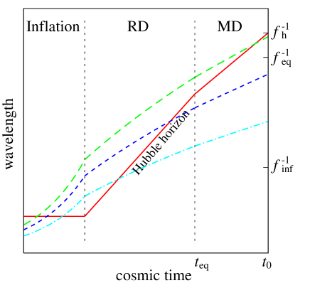
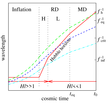
Figure 1: Schematic diagrams of the evolution histories of GWs. Left : four-dimensional case, Right : five-dimensional case. In the high-energy RD regime of the latter case (denoted by “H”), the $\rho^{2}$-term in the Friedmann equation changes the time dependence of the Hubble parameter. This fact yields a new characteristic frequency $f_{\rm crit}$.

II.2 High-energy effects in the braneworld cosmology

In a braneworld scenario, the propagation of gravity may be modified by the presence of extra-dimensional spaces, which affects the observed spectrum of IGWB. In this paper, we consider the Randall-Sundrum single-brane model Randall and Sundrum (1999). In this model, a three-dimensional brane is embedded in five dimensional anti-de Sitter spacetime (AdS₅ bulk) with the curvature scale $\ell$. Here we consider the flat Friedmann-Robertson-Walker (FRW) universe on the brane. In general, the RS model may possess a black-hole in the bulk, but we do not consider it.

II.2.1 Cosmological Expansion on the Brane

In the RS model, the $\mathbb{Z}_{2}$ symmetry (mirror symmetry) is imposed on the brane, whose physical meaning comes from the $S^{1}/\mathbb{Z}_{2}$ orbifold compactification in heterotic M-theory. This symmetry provides the junction condition which gives a relation between the extrinsic curvature $K_{\mu\nu}$ at the brane and the energy density of matter on the brane. From the junction condition, the Friedmann equation on the brane and the conservation law become Mukohyama (2000); Binetruy et al. (2000a, b); Langlois et al. (2000); Kraus (1999); Ida (2000):

$$H^{2}(t)=\left(\frac{\dot{a}}{a}\right)^{2}=\frac{\kappa_{4}^{2}}{3}\rho\left(1+\frac{\rho}{2\lambda}\right),\qquad\dot{\rho}=-3(\rho+p)H,$$ (14)

where $\kappa_{4}^{2}$ represents the gravity constant defined as $\kappa_{4}^{2}=8\pi G=8\pi/M_{\text{pl}}^{2}$ and $\lambda$ denotes the tension of the brane. The tension is related with the bulk curvature scale $\ell$ as $\kappa_{4}^{2}\lambda\ell^{2}=6$ if we require that the cosmological constant on the brane $\Lambda_{4}$ vanishes. For later convenience, we define a dimensionless energy density normalized by the tension $\epsilon(t)$ by $\epsilon(t)\equiv\rho(t)/\lambda$.

From (14), we can separate the regime into two parts : the high-energy regime ($H\ell>1$) and the low-energy regime ($H\ell<1$). The critical energy density satisfying the relation $H\ell=1$ is given by

$$\epsilon_{\rm crit}=\sqrt{2}-1.$$ (15)

Thus, when $\epsilon(t)\gg\epsilon_{\rm crit}$, the high-energy correction characterized by the $\rho^{2}$-term in (14) significantly modifies the cosmological expansion.

In the cosmology with perfect fluid, the exact solutions for the scale factor $a(t)$ and the normalized energy density $\epsilon(t)$ are known. These solutions are expressed as (e.g., Binetruy et al. (2000a, b)):

$$a(t)=\left(\frac{\epsilon_{\rm crit}}{\epsilon}\right)^{1/3(1+w)},\quad\epsilon(t)=\frac{2}{\left\{3(1+w)t/\ell+1\right\}^{2}-1},$$ (16)

where the scale factor is normalized to unity at the critical energy, $\epsilon_{\rm crit}$. In cases with $w=0$ (MD), $w=1/3$ (RD) and $w=1$, the energy densities become respectively

$$\epsilon(t)=\begin{cases}\displaystyle\frac{2\ell^{2}}{9t^{2}+6t\ell}&\;{\rm for}\;\;w=0,\\ \displaystyle\frac{\ell^{2}}{8t^{2}+4t\ell}&\;{\rm for}\;\;w=1/3,\\ \displaystyle\frac{\ell^{2}}{18t^{2}+6t\ell}&\;{\rm for}\;\;w=1.\end{cases}$$ (17)

Using the above relations, we will consider how the high-energy regime of the universe can modify the spectrum of the IGWB.

II.2.2 High-energy effects on GWs

As we mentioned in Sec. I, there are two important effects on the spectrum in the high-energy regime. Let us first consider the non-standard cosmological expansion in presence of $\rho^{2}$-term. From (16), the power-law index of the scale factor in the high-energy regime (‘H’ in the right panel of Fig. 1) is related to the EOS parameter $w$ as

$$n=\displaystyle\frac{1}{3(1+w)}\;\;{\rm for}\;\;t\ll\ell.$$ (18)

On the other hand, at the late-time phase ($\epsilon\ll\epsilon_{\rm crit}$), the power-law index just coincides with the four-dimensional result (11). As a result, the energy spectrum (9) is modified to

$$\Omega_{\rm GW}=\begin{cases}\displaystyle f^{\frac{6w-2}{3w+1}}&{\rm for}\;\;f\ll f_{\rm crit},\\ \displaystyle f^{\frac{6w+2}{3w+2}}&{\rm for}\;\;f\gg f_{\rm crit},\end{cases}$$ (19)

where $f_{\rm crit}$ denotes the critical frequency given by

$$f_{\rm crit} =\frac{1}{2\pi\ell}\frac{a_{\rm crit}}{a_{\rm eq}}\frac{a_{\rm eq}}{a_{0}}$$ (20)

$$=5.6\times 10^{-5}\;{\rm Hz}\left(\frac{\ell}{0.1\;{\rm mm}}\right)^{-1/2}\left(\frac{H_{0}}{72\;{\rm km}/{\rm s}\cdot{\rm Mpc}}\right)^{1/2}\left(\frac{1+z_{\rm eq}}{3200}\right)^{-1/4}.$$

That is, the wavelength at the horizon re-entry time just coincides with the curvature scale, namely, $H_{*}=\ell^{-1}$ (cf. Hogan (2000)). Note that the curvature radius $\ell$ is constrained to $\ell<0.1$ mm by table-top experiments on the Newton force law Chiaverini et al. (2003); Long et al. (2003). For the frequency $f>f_{\rm crit}$, GWs re-enter the horizon during the RD phase of the $\rho^{2}$-term dominated epoch (right panel of Fig. 1). In the high-energy RD phase, the spectrum of the IGWB is modified to

$$\Omega_{\rm GW}\propto f^{4/3}\qquad(f_{\rm crit}<f<f_{\rm inf}),$$ (21)

which is shown in short-dashed lines in Fig 2. Additionally, the inflationary cut-off frequency (3) is modified to

$$f_{\rm inf} \approx\frac{1}{2\pi}\frac{a_{\rm inf}}{a_{\rm crit}}\frac{a_{\rm crit}}{a_{\rm eq}}\frac{a_{\rm eq}}{a_{0}}H_{\rm inf}$$ (22)

$$=4.7\times 10^{6}\;{\rm GHz}\left(\frac{H_{\rm inf}}{6\times 10^{-5}M_{\rm pl}}\right)^{3/4}\left(\frac{H_{0}}{72\;{\rm km}/{\rm s}\cdot{\rm Mpc}}\right)^{1/2}\left(\frac{\ell}{0.1\;{\rm mm}}\right)^{1/4}\left(\frac{1+z_{\rm eq}}{3200}\right)^{-1/4}.$$

Notice that the above estimate neglects another remarkable high-energy effect caused by the excitation of Kaluza-Klein modes (KK-modes). The KK-modes can propagate into the bulk and may be observed on the brane as massive gravitons. By contrast, the GW propagating on the brane is called the ’zero-mode’, and it behaves like a massless graviton on the brane. Strictly speaking, the KK-modes and zero-mode are coordinate-dependent concepts and are mathematically well-defined only in the case of the Minkowski brane and the de-Sitter brane. Nevertheless, we keep to use these terms in the FRW case to distinguish these propagation features.

As we will see in the next section, the brane is generally moving in the bulk spacetime. From the analogy of the moving mirror problem Birrell and Davies (1982), even if only the zero-mode is generated in the inflationary epoch, the zero-mode is partially transferred to KK-modes with the arbitrary masses. If this is true, the amplitude of the zero-mode observed on the brane may be suppressed in comparison with the result neglecting the KK-modes, i.e., (21). The envisaged spectrum involving the two effects is schematically shown as solid lines in Fig. 2. Unfortunately, we cannot fully estimate the KK-mode effects in an analytic way. Thus, in order to construct the IGWB spectrum including the KK-mode effects, we must directly solve the evolution equations of GWs in the five-dimensional cosmology.

In the next section, we present the formalism to solve the evolution equations for GWs numerically.

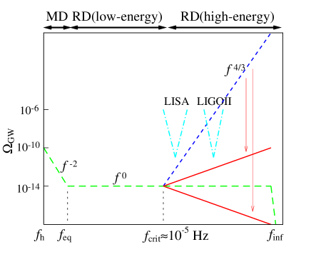
Figure 2: A schematic diagram of the spectrum of IGWB. The four-dimensional prediction is shown in long-dashed lines. Considering the modification due to the non-standard cosmological expansion, the spectrum behaves as $\Omega_{\rm GW}\propto f^{4/3}$ shown in short-dashed line, which may appear upon the detection limit of advanced LIGO (dot-dashed line). Moreover, KK-mode excitations modify the spectrum as solid lines. The main issue in this paper is to clarify whether the resultant spectrum (solid) exceeds the four-dimensional prediction (long-dashed).

III Evolution equation and initial conditions

III.1 Evolution equation of GWs

Let us consider the tensor perturbations in the AdS₅ spacetime. In the Poincaré coordinate $(\tau,\mathbf{x},z)$, the perturbed metric of the AdS₅ spacetime is given by

$$ds^{2}=\left(\frac{\ell}{z}\right)^{2}\{-d\tau^{2}+(\delta_{ij}+h_{ij})dx^{i}dx^{j}+dz^{2}\},\qquad(i,j=1,2,3),$$ (23)

where $h_{ij}$ satisfies the transverse-traceless (TT) condition,

$$\partial_{i}h^{i}{}_{j}=h^{i}{}_{i}=0.$$ (24)

While this coordinate system is free from the coordinate singularities, the brane is non-static, moving in the AdS₅ spacetime Kraus (1999); Ida (2000). The trajectory of the moving brane is determined from the scale factor on the brane, which is described as $(\tau_{\rm b},\,z_{\rm b})$:

$$\tau_{\rm b}=T(t),\qquad z_{\rm b}=\frac{\ell}{a(t)},$$ (25)

where we use the cosmic time $t$ on the brane as a parameter of the trajectory. The function $T(t)$ is given by Deffayet (2002)

$$\dot{T}(t)=\frac{1}{a}\sqrt{1+(H\ell)^{2}}.$$ (26)

In Fig. 3, we show the trajectory denoted by ’Friedmann brane’ in the conformal chart where the surfaces of $\tau=$ const. and $z=$ const. are plotted as dashed lines. One can check that this trajectory induces the metric of the four-dimensional flat Friedmann-Robertson-Walker model on the brane : $ds_{\text{b}}=-dt^{2}+a^{2}(t)\delta_{ij}dx^{i}dx^{j}$. Note that, in the case of de Sitter brane, the scale factor becomes $a(t)=e^{Ht}$ and the Hubble parameter $H$ is constant. Hence the trajectory becomes

$$\tau^{\rm dS}_{\rm b}=-\frac{\sqrt{1+(H\ell)^{2}}}{H}e^{-Ht},\qquad z^{\rm dS}_{\rm b}=\ell e^{-Ht},$$ (27)

which yields the straight trajectory in the bulk; that is, $\tau^{\rm dS}_{\rm b}$ becomes proportional to $z^{\rm dS}_{\rm b}$.

Let us focus on the evolution of the tensor perturbations $h_{ij}$. For convenience, we decompose the quantity $h_{ij}$ into the three-dimensional spatial Fourier modes as

$$h_{ij}(\tau,\mathbf{x},z)=\sum_{P}\int\!h^{P}_{k}(\tau,z)e^{i\mathbf{k}\cdot\mathbf{x}}\hat{e}^{P}_{ij}\,d^{3}k,$$ (28)

where $\hat{e}^{P}_{ij}$ denotes a transverse-traceless polarization tensor. In terms of the Fourier modes, the evolution equation for the perturbations is given by Koyama (2004)

$$\Box_{{\rm AdS}_{5}}h=\frac{\partial^{2}h}{\partial\tau^{2}}-\frac{\partial^{2}h}{\partial z^{2}}+\frac{3}{z}\frac{\partial h}{\partial z}+k^{2}h=0.,$$ (29)

where $\Box_{{\rm AdS}_{5}}$ denotes the d’Alembertian operator in the AdS₅ spacetime. Hereafter we omit subscripts of $h_{k}^{P}$ and simply write $h$. The equation (29) must be solved with the junction condition imposed on the brane. In the Poincaré coordinate, the explicit form of the junction condition becomes Koyama (2004)

$$\left.\frac{\partial h}{\partial n}\right|_{\rm brane}=\left(\frac{\partial h}{\partial\tau}-\frac{\sqrt{1+H^{2}\ell^{2}}}{H\ell}\frac{\partial h}{\partial z}\right)_{z=z_{\rm b}(t)}=0,$$ (30)

where $\partial/\partial n$ denotes the normal vector of the brane. While there is generally a contribution from the tensor part of anisotropic stress tensor on the brane $\pi_{ij}^{\rm T}$, we neglect it for simplicity and set $\pi_{ij}^{\rm T}=0$ hereafter.

It is important to note that the evolution equation (29) can be written in a separable form and by using this fact, one obtains the general solutions (e.g. Gorbunov et al. (2001); Koyama (2004))

$$h(\tau,z)=\int_{0}^{\infty}dm\,\,\left\{\tilde{h}_{1}(m)\,z^{2}\,H_{2}^{(1)}(mz)\,e^{i\,\omega\,\tau}+\tilde{h}_{2}(m)\,z^{2}\,H_{2}^{(2)}(mz)\,e^{-i\,\omega\,\tau}\right\},$$ (31)

where $\omega^{2}=m^{2}+k^{2}$. The functions $H_{2}^{(1)}$ and $H_{2}^{(2)}$ denote respectively the Hankel functions of first and second kind, and $\tilde{h}_{1}(m)$ and $\tilde{h}_{2}(m)$ represent arbitrary coefficients. The above expression implies that the GWs propagating in the bulk are described as a superposition of the zero mode ($m=0$) and the KK-modes ($m>0$). Solving the wave equation (29) with the junction condition (30) is the equivalent task to determining the coefficients $\tilde{h}_{1,2}(m)$ that satisfy the junction condition Koyama (2004). In the very high-energy case, technical difficulties hinder efforts to calculate these analytically because of the significant contribution from the massive modes ($m\ell\gg 1$). For this reason, we solve numerically the wave equation (29) with the junction condition (30).

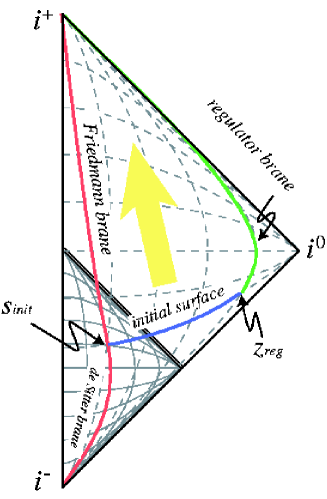
Figure 3: The motion of the de Sitter and Friedmann brane in the AdS₅ bulk in the Poincaré coordinate system.

III.2 Initial conditions

In order to correctly estimate the effects of the KK-modes, we must specify the initial conditions for the perturbed quantity $h$ after the inflation. In this paper, we specifically consider a brane inflation model in which the exponential expansion takes place on the brane. According to Ref. Langlois et al. (2000), the GN coordinate system $(t,\mathbf{x},y)$ provides a useful spatial slicing in the inflationary epoch. With this coordinate, the perturbed metric of the AdS₅ spacetime becomes

$$ds^{2}=-N^{2}(y,t)dt^{2}+A^{2}(y,t)(\delta_{ij}+h_{ij})dx^{i}dx^{j}+dy^{2},$$ (32)

where $A(t,y)=e^{Ht}N(y)$ and $N(t,y)=N(y)=\cosh(y/\ell)-\left(1+\rho/\lambda\right)\sinh(y/\ell)$. Note that the perturbations $h_{ij}$ satisfies the TT conditions (24). In this coordinate, our brane is located at a fixed point $y=0$.

During de Sitter inflation, the solution of the evolution equation of GWs, $\Box_{{\rm AdS}_{5}}h=0$ [see Eq. (29)], can be obtained in a separable form, $h(t,y)\equiv u(y)\phi(t)$. Introducing the separation constant $m$ which represents the mass of KK-modes, the mode functions $u$ and $\phi$ satisfy the following equations Langlois et al. (2000):

$$\frac{d^{2}\phi_{m}}{dt^{2}}+3H\frac{d\phi_{m}}{dt}+\left(m^{2}+\frac{k^{2}}{a^{2}}\right)\phi_{m}=0,$$ (33)

$$\frac{d^{2}u_{m}}{dy^{2}}+4\frac{N^{\prime}}{N}\frac{du_{m}}{dy}+\frac{m^{2}}{N^{2}}u_{m}=0,$$ (34)

where a prime denotes a derivative with respect to $y$. Picking up the normalizable modes from the solutions of the equation (34), one notice that a large mass gap arises between the lightest KK-mode ($m=3H/2$) and the zero-mode ($m=0$) Langlois et al. (2000). From the point of view of the quantum theory, the large mass gap highly suppresses the excitation of KK-modes during inflation. Consequently, the zero-mode solution in the GN coordinates gives a dominant contribution to the metric fluctuation Langlois et al. (2000). Solving the equations (33) and (34) with $m=0$, the zero-mode is described explicitly as

$$h(\eta,y)=C(-k\eta)^{3/2}H_{3/2}^{(1)}(-k\eta),$$ (35)

where $C$ is a normalization constant and $\eta$ is the conformal time $\eta=-1/aH$.

To see how the solution (35) looks like in the Poincaré coordinates, we rewrite the general solution (31) in the GN coordinates. In the de Sitter case, the coordinate transformation between the GN coordinates and the Poincaré coordinates is explicitly given as Gorbunov et al. (2001); Kobayashi et al. (2003)

$$z=-\eta\sinh(y/\ell),\qquad\tau=\eta\cosh(y/\ell),$$ (36)

Substituting them into the general solution (31), we obtain

$$h(\tau,z) = \int_{0}^{\infty}dm\,\left\{\eta\sinh(y/\ell)\right\}^{2}\left\{\tilde{h}_{1}(m)\,H_{2}^{(1)}\left(m\eta\sinh(y/\ell)\right)\,\,e^{-i\,\omega\,\eta\cosh(y/\ell)}\right.$$ (37)

$$\left.~{}~{}~{}~{}~{}~{}~{}~{}~{}~{}+\tilde{h}_{2}(m)\,H_{2}^{(2)}\left(m\eta\sinh(y/\ell)\right)\,\,e^{i\,\omega\,\eta\cosh(y/\ell)}\right\}.$$

Comparing (35) with (37), we see that the zero-mode solution given in the inflationary epoch cannot be simply expressed in terms of the zero-mode solution in the Poincaré coordinates, which indicates that a mixture of KK-modes is required to express the zero-mode solution in the inflationary epoch. Nevertheless, in the long-wavelength limit $k\to 0$, both the zero-mode solutions become constant over the time and the bulk space, and they coincide with each other. Since we are specifically concerned with the evolution of long-wavelength GWs after inflation, the constant mode, i.e., $h=\text{const.}$ and $dh/d\tau=0$, seems a natural and a physically plausible initial condition for our numerical calculation in the Poincaré coordinate. Strictly speaking, however, this is valid only in the long-wavelength limit $k\to 0$. This point will be discussed in details in Sec V.2.

IV Numerical simulation

IV.1 Numerical scheme

On the basis of the formalism presented in the previous section, we now discuss the numerical treatment used to solve the wave equation (29) with the junction condition (30). First of all, the computational domain should be finite. We introduce an artificial cutoff (regulator) boundary in the bulk at $z=z_{\rm reg}$ (shown in Fig. 3) and impose the Neumann condition at the regulator boundary, i.e.,

$$\left(\frac{\partial h}{\partial z}\right)_{z=z_{\rm reg}}=0.$$ (38)

In this paper, numerical calculations were carried out by employing the pseudo-spectral method Canuto et al. (1988). The amplitude of GWs $h(\tau,z)$ is decomposed in terms of Tchebychev polynomials, defined as

$$T_{n}(\xi)\equiv\cos(n\cos^{-1}(\xi))\;\;{\rm for}\;\;-1\leq\xi\leq 1,$$ (39)

which yields a polynomial function of $\xi$ of order $n$. For example,

$$T_{0}(\xi)=1,\quad T_{1}(\xi)=\xi,\quad T_{2}(\xi)=2\xi^{2}-1,\cdots$$ (40)

Here the variable $\xi$ is related to the Poincaré coordinate z. To implement the pseudo-spectral method, instead of using the Poincaré coordinates $(\tau,z)$ directly, we use the new coordinates $(t,\xi)$:

$$\tau=T(t),\qquad z=\frac{1}{2}\left[\,\left\{z_{\rm reg}-z_{\rm b}(t)\right\}\xi+\left\{z_{\rm reg}+z_{\rm b}(t)\right\}\,\,\right]$$ (41)

so that the locations of both the physical and the regulator branes are kept fixed, and the spatial coordinate $z$ is projected to the compact domain $-1\leq\xi\leq 1$. Adopting this coordinate system, the amplitude $h(t,\xi)$ is first transformed into the Tchebychev space through the relation,

$$h(t,\xi)=\sum^{N}_{n=0}\widetilde{h}_{n}(t)T_{n}(\xi),$$ (42)

where we set $N=2048$ or $4096$. We then discretize the $\xi$-axis to the $N+1$ points (collocation points) using the inhomogeneous grid $\xi_{n}=\cos(n\pi/N)$ called Gauss-Lobatto collocation points. With this grid, fast Fourier transformation can be applied to perform the transformation between the amplitude $h(t,\xi)$ and the coefficients $\widetilde{h}_{n}(t)$. Then the wave equation (29) rewritten in the new coordinates are decomposed into a set of ordinary differential equations (ODEs) for $\widetilde{h}_{n}(t)$. For the temporal evolution of $\widetilde{h}_{n}(t)$, we use Adams-Bashforth-Moulton method with the predictor-corrector scheme. Further technical details of the numerical scheme is summarized in Appendix A.

IV.2 Setup and parameters

We are especially concerned with the late-time evolution of GWs after the inflation. For this purpose, we focus on the evolution equation (29) in the RD phase. In order to quantify high-energy effects, we define a useful parameter $\epsilon_{*}$ which represents the normalized energy density at the horizon re-entry time $t_{*}$ of the GWs concerned, namely, $\epsilon_{*}=\epsilon(t_{*})$. From the Friedmann equation (14) and the definition of the scale factor (16), the comoving wave number of GWs is rewritten in terms of the parameter $\epsilon_{*}$ as

$$k=a_{*}H_{*}=\left(\frac{\epsilon_{\rm crit}}{\epsilon_{*}}\right)^{1/3(1+w)}\sqrt{\epsilon_{*}^{2}+2\epsilon_{*}}.$$ (43)

For higher frequency GWs, $\epsilon_{*}$ becomes larger. One thus expects that the high-frequency GW modes tend to be significantly affected by the high-energy effects.

Notice that the location of the regulator brane is another important parameter. Here, the location of the boundary is set to $z_{\rm reg}=25$–$200\ell$, which is far enough away from the physical brane to avoid artificial suppression of light KK-modes. Further, we must stop the numerical calculations before the influence of the boundary condition at $z=z_{\rm reg}$ reaches the physical brane $z_{\rm b}$. The arrival time of the influences of the regulator brane can be estimated by drawing a null line from the initial position of the regulator boundary $(\tau_{0},z_{\rm reg})$ toward the physical brane. With these treatments, we have checked that the amplitude of GWs on the brane is fairly insensitive to the location of regulator boundaries. Thus, all the results presented in Sec. V and Sec. VI are free from the effect of regulator boundary.

In the situation considered here, the initial time $t_{\rm init}$ is also an important parameter, which turns out to have an important effect on the GWs in the bulk Hiramatsu et al. (2005). We parameterize the initial time as

$$s_{\rm init}\equiv\frac{a(t_{\rm init})H(t_{\rm init})}{k},$$ (44)

which represents the wavelength of GWs normalized by the Hubble horizon scale at the initial time $t_{\rm init}$. In order to get a reliable estimate, we set $s_{\rm init}\gg 1$ and run the simulations until $\epsilon(t)\ll 1$, when the high-energy effects on the GWs become negligible.

Finally, we adopt the constant mode $h(t_{\rm init},\xi)=1$ as an initial condition according to the discussion in Sec. III.2. Although it is plausible, the validity of the constancy of the superhorizon modes must be checked. This point will be carefully discussed in Sec. V.2.

V Code check and qualitative behavior of GWs

V.1 Code check

In order to check our numerical code, we first consider the simplest case in which the location of the brane is given by $z=z_{\rm b}=$constant. This is the so-called Minkowski brane embedded in the AdS₅ bulk. The solution of the evolution equation (29) is given as Randall and Sundrum (1999); Sasaki et al. (2000); Gorbunov et al. (2001)

$$h_{\rm exact}(\tau,z)=z^{2}Z_{2}(mz)E(\omega\tau),$$ (45)

where $\omega\equiv\sqrt{k^{2}+m^{2}}$. The function $Z_{2}$ and $E$ respectively denote linear combinations of the Bessel functions of order 2 and the sinusoidal functions. Imposing the junction condition (30) at $z_{\rm b}=\ell$, we obtain

$$h_{\rm exact}(\tau,z)=\left(\frac{z}{\ell}\right)^{2}\left\{Y_{1}(m)J_{2}(mz)-J_{1}(m)Y_{2}(mz)\right\}\cos(\omega\tau).$$ (46)

According to the analytic solution (46), we set $h=h_{\rm exact}(0,z)$ and $\dot{h}=\partial h_{\rm exact}/\partial\tau|_{\tau=0}=0$ for the initial condition of numerical simulation and compare the numerical results with the analytic solution.

Fig. 4 shows the behavior of GWs in the AdS₅ bulk. The right panel of the figure is the projection of the left panel. In this simulation, we chose parameters as $z_{\rm reg}=20\ell$, $m\ell=k\ell=2$ and $N=1024$. The left panel of Fig. 5 shows the snapshot of the waveform at $\tau=\tau_{1}=10\ell$, which illustrates that the numerical result accurately recovers the exact solution (46) in the interval between $z_{\rm b}\leq z\leq z_{\rm reg}-\tau_{1}$. Outside this region, the numerical simulation is contaminated by the boundary condition of the regulator brane. In the right panel of Fig. 5, the fractional error of the amplitude $|(h_{\rm num}-h_{\rm exact})/h_{\rm exact}|$ evaluated at the time $\tau=\tau_{1}$ is plotted as a function of bulk coordinate. We found that the error is suppressed to the order of $10^{-3}$ near the physical brane. Note that there appear several sharp spikes, whose locations roughly match those of the zero-point $h_{\rm exact}(\tau,z)=0$. Thus, the cancellation of significant digits occurs. These numerical errors can be reduced when the number of collocation points $N$ is increased.

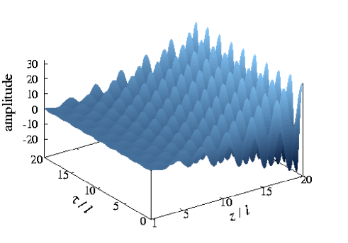
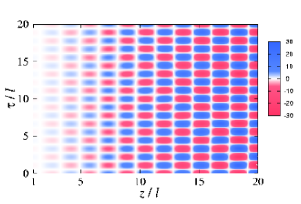
Figure 4: The behavior of a test wave with $m\ell=k\ell=2$ in the bulk. The Minkowski brane is located at $z=\ell$. The right panel depicts the projection of the three-dimensional waves of the left panel.

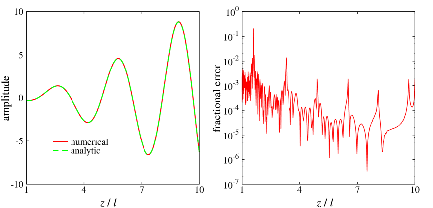
Figure 5: The left panel illustrates that the numerical solution at $\tau=10$ is consistent with the analytical solution (46) in the region $z_{\rm b}\leq z\leq 10$. The outer region $10\leq z\leq z_{\rm reg}$ in the bulk is contaminated by the boundary condition on the regulator brane at $z=z_{\rm reg}$. The right panel shows the numerical errors $|(h_{\rm num}-h_{\rm exact})/h_{\rm exact}|$ estimated at that time, which is suppressed by $10^{-3}$ near the physical brane. The spike-shapes reflects the cancellation of significant digits because of $h_{\rm exact}(10,z)\approx 0$.

V.2 Behavior of GWs in the bulk and the validity check of the initial condition

Having checked the reliability of our numerical scheme, we now focus on the cosmological evolution of GWs. As we mentioned in Sec III.2, we must first clarify the validity and the sensitivity of the initial condition, namely, the constancy of the superhorizon modes. It should be stressed that, only in the long-wavelength limit $k\to 0$ during the inflationary phase, the constant mode coincides with the zero-mode solution [see Eq.(37)]. Therefore, the constancy of GW amplitudes after inflation cannot be guaranteed even on superhorizon scales. Depending on the choice of the parameters $s_{\rm init}$ and $\epsilon_{*}$, the mode $h=$ const. may not be a good approximation to the initial condition for numerical simulations in the RD epoch.

Fig. 6 shows the time evolution of GWs in the Poincaré coordinate system in the de Sitter case. In this simulation, we set $s_{\rm init}=100$ and $H\ell=\sqrt{3}$. The universe on the brane experiences accelerated cosmological expansion and the wavelength of GWs becomes longer than the Hubble horizon. Fig. 6 indicates that the GWs on initially superhorizon-scale remains constant not only on the brane but also in the bulk. The right panel of this figure, which depicts the projection of the left panel, shows that a very slight change of the amplitude is observed (a fraction of the original amplitude of $\leq 1\%$) and the amplitude finally converged to a fixed value. In this sense, the constant mode $h=const$. is suitable for the initial condition of the superhorizon-scale GWs in the RD phase if we impose the initial condition just after the inflation.

Adopting this initial condition, we then performed simulations in the radiation-dominated FRW case $(w=1/3)$ with same parameters, $\epsilon_{*}=1.0$ and $s_{\rm init}=100$. This result is shown in Fig 7. We found that the constancy of the GW amplitude no longer holds in the bulk even before $\tau\approx 0$, where the wavelength of GW on brane just re-enters the Hubble horizon. In particular, GWs emanating from the physical brane are observed, which propagate into the bulk spacetime almost along a null line. This indicates that the excitation of KK-modes occurs near the brane even if the wavelength of GWs is still outside the Hubble horizon.

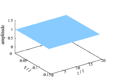
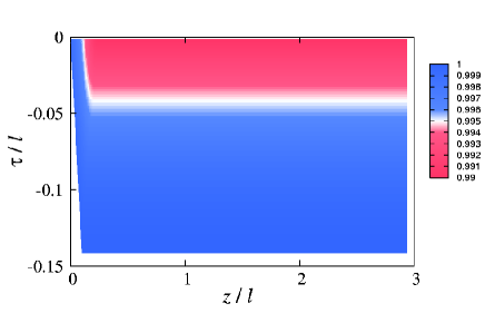
Figure 6: The evolution of a GW in the bulk in the case of a de Sitter brane. We set the Hubble parameter to $H\ell=\sqrt{3}$ with $(s_{\rm init},z_{\rm reg})=(10,20)$. The right panel depicts the projection of the three-dimensional waves of the left panel, zooming in the image in $0\leq z/\ell\leq 3$. The empty corner in the surface represents the motion of the brane [see Eq.(27)].

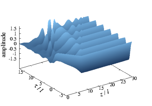
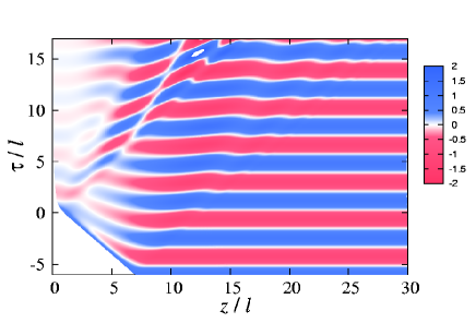
Figure 7: The evolution of a GW in the bulk in the case of a Friedmann brane. We set the comoving wave number to $k=\sqrt{3}/\ell$ or $\epsilon_{*}=1.0$ with $(s_{\rm init},z_{\rm reg})=(200,80)$. The right panel depicts the projection of the three-dimensional waves of the left panel. The empty corner in the surface represents the motion of the brane [see Eq.(25)].

It is noteworthy that the different behaviors of GWs in the AdS₅ bulk may be caused by the difference in the motion of the brane [see Eqs.(25) and (27)]. In the moving mirror problem in an electromagnetic field, the acceleration or deceleration of the mirror yields the creation of photons due to vacuum polarization (e.g., Sec. 4.4 of Ref. Birrell and Davies (1982)). A similar phenomenon may occur in the AdS₅ bulk, that is, the KK-modes (massive gravitons) are excited by the deceleration of the brane which is depicted by an arc with a non-zero curvature $d^{2}z_{\rm b}/d\tau^{2}<0$.

Figs. 6 and 7 reveal that the constant mode $h(t_{\rm init},\xi)=\text{const.}$ can be used as the initial condition if we set this just after the end of inflation, but, the constancy of the long-wavelength mode would not be guaranteed in the RD epoch even on superhorizon scales. This implies that the choice of the initial time $t_{\rm init}$ (or $s_{\rm init}$) defined in (44) is crucial when setting the initial condition at the RD epoch.

In Figs. 8 and 9, the dependence of the evolution of GWs on the initial time is shown by varying the parameter $s_{\rm init}$ in low-energy ($\epsilon_{*}=0.1$) and high-energy ($\epsilon_{*}=10$) cases. Fig. 8 plots the snapshots of the amplitude $h(\tau,z)$ in the bulk when the wavelength of GWs becomes five times larger than the Hubble horizon, i.e., $aH/k=5$. Clearly, in the bulk, the amplitude of GWs is very sensitive to the choice of the parameter $s_{\rm init}$, or equivalently, the initial time $t_{\rm init}$. The resultant wave-form away from the physical brane does not show any convergence even in the low-energy case $(\epsilon_{*}=0.1)$. This behavior may be caused by the fact that the constant mode with the comoving wave number $k$ in the RD epoch immediately starts to oscillate as $h(\tau,z)\propto e^{ik\tau}$, which is the massless ($m\to 0$) limit of Eq. (31).

On the other hand, in Fig. 9, the GW amplitudes tend to converge on the brane if we set the initial time $t_{\rm init}$ early enough. This convergence property might be due to the presence of the junction condition (30). Therefore, as far as we choose $s_{\rm init}\gtrsim 50$ for our interest of the energy scale $0.01\lesssim\epsilon_{*}\lesssim 100$, we do not need to care about the initial time, when we estimate the IGWB spectra on the brane. In Appendix B, quantitative aspects of the convergence properties of the amplitude are discussed. Moreover, Seahra addressed these points in an analytic way in Ref.Seahra (2006).

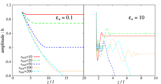
Figure 8: Snapshots of the GW amplitudes in the bulk for various choices of initial time. The snapshots were taken when the wavelength of GWs becomes five times longer than the Hubble horizon, i.e., $aH/k=5$.

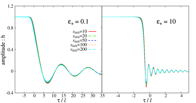
Figure 9: Evolved results of GWs projected on the brane starting with the various initial times.

VI IGWB spectra

VI.1 Comparison with reference waves

Keeping the results in Sec. V in mind, let us now quantitatively estimate the high-energy effects of the GWs and evaluate the energy spectra of the IGWB on the brane. To quantify these, it might be helpful to discriminate the influence of KK-mode excitation in the bulk from the non-standard cosmological expansion caused by the $\rho^{2}$-term in the Friedmann equation (14). For this purpose, we introduce the reference wave $h_{\rm ref}$, which is a solution of the four-dimensional evolution equation of the amplitude obtained by replacing the scale factor and the Hubble parameter derived from the standard Friedmann equation with those from the modified Friedmann equation (14). The resultant equation is given by

$$\ddot{h}_{\rm ref}+3H\dot{h}_{\rm ref}+\left(\frac{k}{a}\right)^{2}h_{\rm ref}=0,$$ (47)

which is just the Klein-Goldon equation for a scalar field in the FRW background (e.g. Allen (1988); Maggiore (2000)) and is same as (33) for $m=0$. Comparing the numerical simulations with the solution of the wave equation (47), the effect of the KK-mode excitation can be quantified separately.

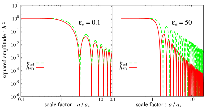
Figure 10: Squared amplitude of GWs on the brane in low-energy (left) and the high-energy (right) regimes. In both panels, solid lines represent the numerical solutions of wave equation (29). The dashed lines are the amplitudes of reference wave $h_{\rm ref}$ obtained from equation (47).

Fig. 10 shows the squared amplitude of the GWs, $h_{\rm 5D}^{2}$ and $h_{\rm ref}^{2}$ as functions of the scale factor $a$. The left panel shows the low-energy case ($\epsilon_{*}=0.1$), while the right panel depicts the result in the high-energy regime ($\epsilon_{*}=50$). As we increase the energy scale at the horizon re-entry time, the GW amplitude $h_{\rm 5D}$ becomes considerably reduced compared to the reference wave, $h_{\rm ref}$. Since the late-time evolution of GWs simply scales as $h\propto 1/a$ in both $h_{\rm 5D}$ and $h_{\rm ref}$, the suppression of the amplitude $h_{\rm 5D}$ is caused by the excitation of KK-modes around the horizon re-entry time. Notice that the normalized energy density at the horizon re-entry time $\epsilon_{*}$ is related to the observed proper frequency $2\pi\,f=k/a_{0}=(a_{*}/a_{0})H_{*}$ as

$$\frac{f}{f_{\text{crit}}}=\left(\frac{a_{*}}{a_{\rm crit}}\right)\ell H_{*}=\left(\frac{\epsilon_{\rm crit}}{\epsilon_{*}}\right)^{1/3(1+w)}\sqrt{\epsilon_{*}^{2}+2\epsilon_{*}},$$ (48)

where the critical frequency $f_{\text{crit}}$ is defined in (20) as $2\pi f_{\text{crit}}=(a_{\rm crit}/a_{0})\ell^{-1}$, and $w=1/3$ in this case. From this relation, one expects that the KK-mode excitation is essential in the high-energy regime and the deviation from the standard four-dimensional prediction for the spectrum of IGWB becomes more prominent above the critical frequency, $f>f_{\rm crit}$.

VI.2 IGWB spectrum in the five-dimensional cosmology

We are in position to estimate the influence of KK-mode excitation on the shape of the spectrum. To do so, we ran simulations for the parameters listed in Table 1 ($w=1/3$ case) and estimated the ratio of amplitudes $|h_{\rm 5D}/h_{\rm ref}|$ for a different set of parameters. Note that in the simulations with $\epsilon_{*}\lesssim 1$, the location of regulator brane $z_{\rm reg}$ should be set far away from the physical brane. This is because the long-term evolution is needed to follow the oscillatory behavior.

We show the frequency dependence of the ratio in Fig. 11. The ratio is evaluated at the low-energy regime long after the horizon re-entry time and is plotted as a function of the frequency $f/f_{\rm crit}$. Clearly, the ratio $|h_{\rm 5D}/h_{\rm ref}|$ monotonically decreases with the frequency and the suppression of amplitude $h_{\rm 5D}$ becomes significant above the critical frequency $f_{\rm crit}$. Using the data points in the asymptotic region $\epsilon_{*}\geq 5$, we try to fit the ratio of amplitudes with $s_{\rm init}=200$ to a power-law function. Employing the least-squares method, the result becomes

$$\left|\frac{h_{\rm 5D}}{h_{\rm ref}}\right|=\alpha\left(\frac{f}{f_{\text{crit}}}\right)^{-\beta}$$ (49)

with $\alpha=0.76\pm 0.01$ and $\beta=0.67\pm 0.01$ (dashed line in Fig. 11). In Appendix B, we calculate the ratios for various $s_{\rm init}$ for each combination $(\epsilon_{*},z_{\rm reg})$ to check the robustness of this result.

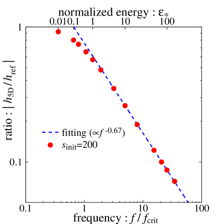
Figure 11: Frequency dependence of the ratio of amplitudes $|h_{\rm 5D}/h_{\rm ref}|$ between the numerical simulation of wave equation (29) and the reference wave (47). The vertical solid line represents the critical frequency. The dashed line indicates the fitting result (49), where fitting was examined using the data with $s_{\rm init}=200$ at the asymptotic region $\epsilon_{*}\geq 5$.

$w$	$(\epsilon_{*},z_{\rm reg})$	$s_{\rm init}$	$N$
0	$(0.1,200\ell)\sim(100,50\ell)$	$50,100,200,400$	2048 or 4096
$1/3$	$(0.01,200\ell)\sim(100,25\ell)$	$50,100,200,400,800$	2048 or 4096
1	$(0.1,500\ell)\sim(50,50\ell)$	$200,400,800,3200,12800$	2048 or 4096

Table 1: Numerical parameters used for the simulations to estimate the frequency dependence of the ratio of amplitudes $|h_{\rm 5D}/h_{\rm ref}|$.

The power-law fit (49) can be immediately translated to the energy spectrum of IGWB, $\Omega_{\rm GW}$. The spectrum taking account of the KK-mode excitations is calculated as

$$\Omega_{\rm GW}=\left|\frac{h_{\rm 5D}}{h_{\rm ref}}\right|^{2}\Omega_{\rm ref},$$ (50)

where we used the fact $\Omega_{\rm GW}\propto h^{2}f^{2}$. As discussed in Sec. II.2.2, if we neglect the effect of the KK-mode excitation, the spectrum becomes $\Omega_{\rm ref}\propto f^{4/3}$ [See Eq.21]. Then, combining it with the result (49), the IGWB spectrum becomes nearly flat above the critical frequency :

$$\Omega_{\rm GW}\propto f^{0},$$ (51)

which is shown in filled squares in Fig. 12. In this figure, the spectrum calculated from the results of the reference waves $\Omega_{\rm ref}$ is also shown in filled circles. Note that the normalization factor of the spectrum is determined so as to be $\Omega_{\rm GW}=10^{-14}$ according to the constraint from the CMB observation. The short-dashed line and the solid line represent each asymptotic behavior in the high-frequency region. The spectrum taking account of the two high-energy effects seems almost indistinguishable from the standard four-dimensional prediction shown in long-dashed line in the figure. In other words, while the effect due to the non-standard cosmological expansion lifts up the spectrum, the KK-mode effect reduces the GW amplitude, which results in the same spectrum as the one predicted in the four-dimensional theory. Additionally notice that the amplitude taking account of the two effects near $f\approx f_{\rm crit}$ is slightly decreasing, which agrees with the results in our previous study for $\epsilon_{*}\leq 0.3$ using the GN coordinates Hiramatsu et al. (2004).

At this point, however, it is unclear whether the results obtained here is generic or accidental for certain range of the model parameters. To clarify the cosmological dependence of the KK-mode excitations in more quantitative way, we next study the cases with different EOS parameter $w$.

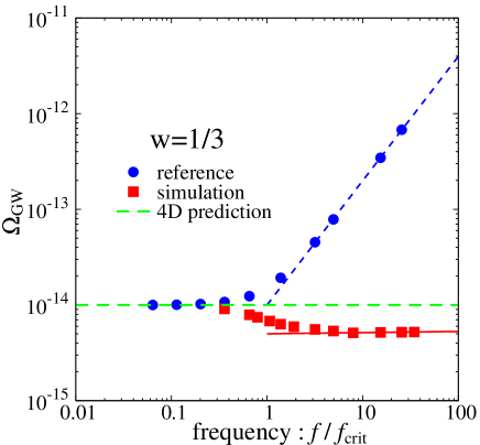
Figure 12: The energy spectrum of the IGWB around the critical frequency. The filled circles represent the spectrum caused by the non-standard cosmological expansion of the universe. Taking account of the KK-mode excitations, the spectrum becomes the one plotted as filled squares. Particularly, in the asymptotic region depicted in the solid line, the frequency dependence becomes almost same as the one predicted in the four-dimensional theory (long-dashed line).

VI.3 Dependence on equation of state

To quantify the EOS dependence, we ran simulations for the MD case $w=0$ and the somewhat stiff matter case $w=1$, which might be realized by introducing the kinetically driven scalar field (e.g. the quintessential inflation Sahni et al. (2002); Sami and Sahni (2004)). Varying the EOS parameter changes the acceleration of the brane. One naively expects that the different motion of the brane may suppress or enhance the KK-mode excitation.

With the same procedure as in the previous subsection, we calculated the ratio of amplitudes $|h_{\rm 5D}/h_{\rm ref}|$ for various $\epsilon_{*}$ in the case of $w=0$ and $w=1$. The results are summarized in Fig. 13, where the horizontal axis represents $\sqrt{1+H_{*}^{2}\ell^{2}}$. Fitting the power-law function to all cases shown in the figure, we found that the ratios universally scale as

$$\left|\frac{h_{\rm 5D}}{h_{\rm ref}}\right|=\widetilde{\alpha}(1+H_{*}^{2}\ell^{2})^{-0.24}\approx\widetilde{\alpha}(1+H_{*}^{2}\ell^{2})^{-1/4},$$ (52)

where $\widetilde{\alpha}=0.75,0.81$ and $0.83$ for $w=0,1/3$ and 1, respectively, which indicates that the quantity $\widetilde{\alpha}$ may be related to $w$ as $\widetilde{\alpha}=-0.155w^{2}+0.241w+0.748$ by simply fitting the quadratic function. An important point to emphasize is that this scaling property does not depend on the parameter $w$ or the acceleration of the brane. Combining the scaling relation with (50), the IGWB spectra can be estimated as

$$\Omega_{\rm GW}=\widetilde{\alpha}^{2}(1+H_{*}^{2}\ell^{2})^{-1/2}\Omega_{\rm ref}.$$ (53)

Especially, in the high-frequency region $f\gg f_{\rm crit}$, the prefactor of the right-hand side behaves as

$$(1+H_{*}^{2}\ell^{2})^{-1/2}\approx H_{*}\ell\propto f^{-\frac{3(w+1)}{3w+2}}$$ (54)

from equations (7),(8) and (18). Combining the result (19), the energy spectrum of the IGWB behaves as

$$\Omega_{\rm GW}\propto f^{\frac{3w-1}{3w+2}}\;\;{\rm for}\;f\gg f_{\rm crit}.$$ (55)

Owing to these calculations (19) and (55), for $w=0$ (MD), we obtain

$$\Omega_{\rm GW}\propto\begin{cases}f^{-1/2}&{\rm for}\;\;f\gg f_{\rm crit},\\ f^{-2}&{\rm for}\;\;f\ll f_{\rm crit},\end{cases}$$ (56)

and for $w=1$ case,

$$\Omega_{\rm GW}\propto\begin{cases}f^{2/5}&{\rm for}\;\;f\gg f_{\rm crit},\\ f^{1}&{\rm for}\;\;f\ll f_{\rm crit}.\end{cases}$$ (57)

These results imply that the spectrum generally changes from the four-dimensional prediction. Indeed, transforming the numerical results (52) to the energy spectra in the cases with $w=0$ and $w=1$, the frequency dependence of the spectra including the two high-energy effects (solid lines) clearly differ from each four-dimensional prediction (long-dashed lines).

Taking these results into account, one may conclude that the cancellation of the high-energy effects in the RD epoch is accidental and the KK-mode excitation dominates over the non-standard cosmological expansion when $w>1/3$.

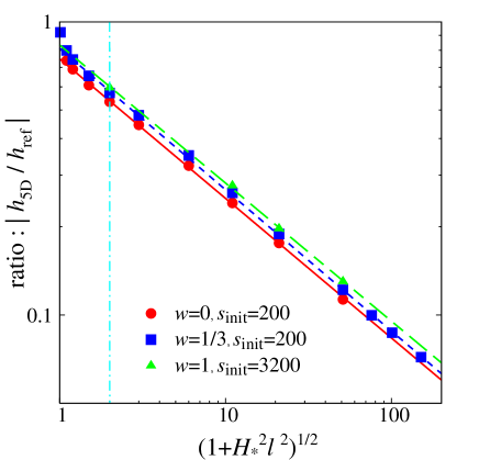
Figure 13: EOS dependence on the amplitude ratio. The filled circles, squares and triangles show the cases with $w=0,1/3$ and $1$, respectively. The solid line, short-dashed line and long-dashed line show each fitting result above the critical frequency corresponding to $(1+H_{\rm crit}^{2}\ell^{2})^{1/2}=\sqrt{2}$ depicted in the vertical dot-dashed line.

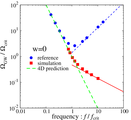
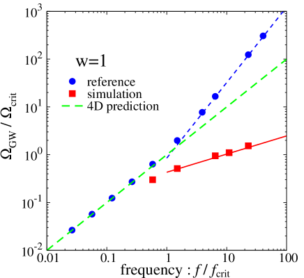
Figure 14: The energy spectrum of the IGWB in the background EOS with $w=0$(left), and with $w=1$(right). The amplitude is normalized by the value of the four-dimensional prediction at the critical frequency.

VII Conclusion

We have investigated the power spectrum of the IGWB in the five-dimensional cosmology based on the Randall-Sundrum model. In the braneworld scenario, the two high-energy effects affect the shape of the spectrum above the critical frequency $f_{\rm crit}$ defined in (20). One is the non-standard cosmological expansion on the brane caused by the high-energy correction of the Friedmann equation. The analytical estimate taking account of this effect reveals that the effect makes the spectrum steeply blue [see Eq. (21)]. By contrast, another important effect is the excitations of KK-modes which escapes from our brane into the five-dimensional bulk, leading to the suppression of the spectrum. In order to quantify these two effects, we solved the wave equation of each Fourier mode of GWs numerically for various EOS parameters $w$.

The systematic survey of numerical simulations with various parameter sets reveals that there may exist the universal scaling law for the KK-mode excitation in the high-energy regime [Eq.(52)]:

$$\left|\frac{h_{\rm 5D}}{h_{\rm ref}}\right|\propto(1+H_{*}^{2}\ell^{2})^{-1/4}.$$

Using the universal scaling law, we constructed the power spectrum of the IGWB in the cases with $w=0$ (MD universe), $w=1/3$ (RD universe) and $w=1$ (stiff matter dominant universe). From the results (12) and (55), the frequency dependence of the spectrum in the high-frequency region $f>f_{\rm crit}$ becomes

$$\Omega_{\rm GW}\propto\begin{cases}f^{-2}\;({\rm 4D})\;,\;f^{-1/2}\;({\rm 5D})&{\rm for}\;\;w=0,\\ f^{0},\;\hskip 30.00005pt\;f^{0}&{\rm for}\;\;w=1/3,\\ f^{1},\;\hskip 30.00005pt\;f^{2/5}&{\rm for}\;\;w=1.\end{cases}$$ (58)

Particularly, in the RD case, the accidental cancellation of the two high-energy effects occurs, which yields the same spectrum as one predicted in the four-dimensional (4D) theory. This scaling law might be understood in a context of moving mirror problems. The discussion about the analytic derivation of the scaling law is work in progress.

Finally, we briefly comment on the other numerical works using the different schemes. Recently, Seahra solved numerically the wave equation in the null coordinate system based on the Poincaré coordinates using a sophisticated numerical scheme Seahra (2006). He observed the agreement between his numerical results and our results for the same choice of the EOS parameters with the same initial conditions as ours. In addition, it is observed that, even if a constant initial condition on the initial null hypersurface is chosen, the amplitude of GWs on the brane is almost identical with our results. Moreover, the numerical calculation based on the quantum theory has been performed by Kobayashi and Tanaka Kobayashi and Tanaka (2005b). They reported the same spectrum in the RD case as ours, even if KK modes are taken into account in the initial de Sitter phase. On the other hand, Ichiki and Nakamura have obtained a tilted spectrum $\Omega_{\rm GW}\propto f^{-0.46}$ Ichiki and Nakamura (2003). While their early results have included errors associated with numerical accuracy, the new calculation using the revised code did not converge to the flat spectrum either. Currently, we do not know the reason why the result by Ichiki and Nakamura is different from ours. In order to understand these numerical results well, the analytical study of the scaling relation (52) is essential, which is definitely our next task.

Appendix A The pseudo-spectral method

In this appendix, we briefly describe the implimentation of the pseudo-spectral method in our numerical scheme.

From the coordinate transformation (41), the wave equation (29) is expressed as

$$\frac{\partial^{2}h}{\partial t^{2}}+K_{t\xi}\frac{\partial^{2}h}{\partial t\partial\xi}+K_{\xi\xi}\frac{\partial^{2}h}{\partial\xi^{2}}+K_{t}\frac{\partial h}{\partial t}+K_{\xi}\frac{\partial h}{\partial\xi}+Kh=0,$$ (59)

where the coefficients $K_{t\xi},K_{\xi\xi},K_{t},K_{\xi}$ and $K$ are functions of $t$ and $\xi$. We use the predictor-corrector method for the temporal evolution. To implement this, we introduce an auxiliary variable $\chi(t,\xi)$ satisfying the equation

$$\frac{\partial h}{\partial t}=\chi-K_{t\xi}\frac{\partial h}{\partial\xi}\equiv F(\chi,h^{\prime};t,\xi_{n}),$$ (60)

where the prime denotes the derivative with respect to $\xi$ [see Eq.(41)]. With this definition, the time evolution of $\chi$ satisfying to (29) is formally written as

$$\frac{\partial\chi}{\partial t}=G(\chi,h,h^{\prime},h^{\prime\prime};t,\xi_{n}).$$ (61)

Notice that the function $G$ does not contain the derivative $\partial\chi/\partial\xi$. Empirically, the presence of this derivative causes numerical instability. The functions $F$ and $G$ are evaluated at each collocation point $\xi_{n}$. Then, transforming to the Tchebychev space by Eq. (42), we obtain a set of ordinary differential equations :

$$\frac{d\widetilde{h}_{n}}{dt}=\widetilde{F}_{n}(t),\;\;\frac{d\widetilde{\chi}_{n}}{dt}=\widetilde{G}_{n}(t).$$ (62)

With the reduced equations (62), the predictor-corrector method based on the Adams-Bashforth-Moulton scheme can be used to obtain the time evolution of $\widetilde{h}_{n}(t)$ and $\widetilde{\chi}_{n}(t)$.

At each time step, while the boundary conditions (30) and (38) are used to evaluate $\widetilde{h}_{N-1}$ and $\widetilde{h}_{N}$, we put additional conditions on $\widetilde{\chi}_{N-1}$ and $\widetilde{\chi}_{N}$ as

$$\widetilde{\chi}_{N-1}=\widetilde{\chi}_{N}=0.$$ (63)

Owing to the definition of the function $F$ containing no derivatives of $\chi$ [see Eq.(60)], this empirically based treatment of boundary conditions suppresses the numerical error caused by finite truncation of the Tchebychev transformation (42).

In summary, we firstly evaluate the functions $F$ and $G$ in the physical space at the time $t$. Then, transforming them into the Tchebychev space by (42), we obtain $\widetilde{h}_{n}$ and $\widetilde{\chi}_{n}$ at the next time step $t+\Delta t$ by solving the reduced equations (62) for $0\leq n\leq N-2$, and imposing the boundary conditions and the additional conditions (63) into $\widetilde{h}_{n}$ and $\widetilde{\chi}_{n}$ for $n=N-1,N$. The spectral coefficients of the derivatives $h^{\prime}$ and $h^{\prime\prime}$ can be computed in decreasing order by the recurrence relations Canuto et al. (1988)

$$c_{n}\widetilde{h}_{n}^{(1)}=\widetilde{h}_{n+2}^{(1)}+2(n+1)\widetilde{h}_{n+1},\qquad\widetilde{h}_{n\geq N}^{(1)}=0,$$ (64)

and then

$$c_{n}\widetilde{h}_{n}^{(2)}=\widetilde{h}_{n+2}^{(2)}+2(n+1)\widetilde{h}_{n+1}^{(1)},\qquad\widetilde{h}_{n\geq N}^{(2)}=0,$$ (65)

where $c_{n}$ is defined as

$$c_{n}=\begin{cases}2&{\rm for}\;\;n=0,N\\ 1&{\rm for}\;\;1\leq n\leq N-1\end{cases}.$$ (66)

Finally, we obtain $h(t+\Delta t,\xi)$ and its derivatives $h^{\prime}(t+\Delta t,\xi)$ and $h^{\prime\prime}(t+\Delta t,\xi)$ by the inverse Tchebychev transformation.

Appendix B Initial time dependence

As seen in V.2, the amplitudes on the brane becomes insensitive to the choice of the initial time as long as $s_{\rm init}$ is large enough. In this appendix, we show that the ratios of amplitudes discussed in VI.2 tend to converge to a fixed value in the low-energy and high-energy cases. This validates the estimation of the power spectrum of the IGWB using the results obtained from the simulations with $s_{\rm init}=200$.

Fig. 15 shows the dependence of the ratios $h_{\rm 5D}/h_{\rm ref}$ on the parameter $s_{\rm init}$. The left and right panels show the high-energy ($\epsilon_{*}=50$) and the low-energy ($\epsilon_{*}=0.1$) cases, respectively. In both cases, the ratios clearly converge to certain asymptotic values as increasing $s_{\rm init}$. Using the nonlinear least-square method, we tried to fit these values to the function

$$\left|\frac{h_{\rm 5D}}{h_{\rm ref}}\right|=As_{\rm init}^{B}+C,$$ (67)

where $A,B,C$ are fitting parameters depending on $\epsilon_{*}$. Then we obtained

$$(A,B,C)=\begin{cases}(0.566,\;-0.573,\;0.772)&{\rm for}\;\;\;\epsilon_{*}=0.1,\\ (0.456,\;-0.880,\;0.118)&{\rm for}\;\;\;\epsilon_{*}=50,\end{cases}$$ (68)

which are shown in solid curves in Fig. (15). Note that $C$ represents the asymptotic values shown in long-dashed lines in each panel.

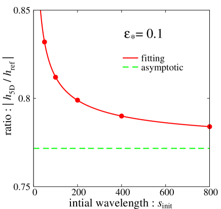
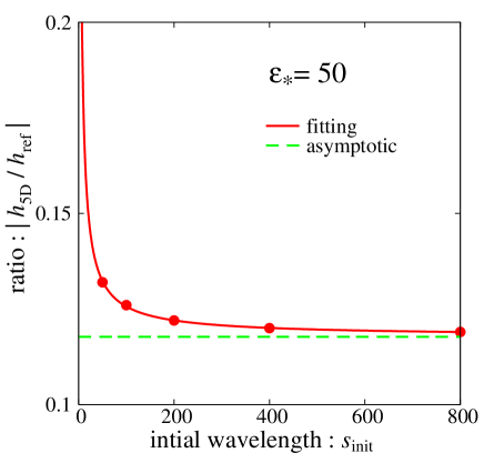
Figure 15: Convergence of the ratio of amplitudes $h_{\rm 5D}/h_{\rm ref}$. Solid lines represent the fitting curve calculated by employing the nonlinear least-square method. Long-dashed lines denote the asymptotic value of the ratio.

Picking up the values at $s_{\rm init}=200$ in both cases, one can see that the deviations from the asymptotic values $C$ keep to be less than a few percent. From this fact, we use the ratios with $s_{\rm init}=200$ to construct the power spectra of the IGWB without deriving the asymptotic values for each $\epsilon_{*}$.

References

- Ando and the TAMA Collaboration (2005) M. Ando and the TAMA Collaboration, Classical and Quantum Gravity 22, 881 (2005).
- Sigg (2004) D. Sigg, Classical and Quantum Gravity 21, 409 (2004).
- Acernese et al. (2005) F. Acernese et al., Classical and Quantum Gravity 22, 869 (2005).
- Grote et al. (2005) H. Grote et al., Classical and Quantum Gravity 22, 193 (2005).
- Abbott et al. (2005) B. Abbott et al., Physical Review Letters 95, 221101 (2005).
- Starobinskii (1979) A. A. Starobinskii, Journal of Experimental and Theoretical Physics Letteres 30, 682 (1979).
- Rubakov et al. (1982) V. A. Rubakov, M. V. Sazhin, and A. V. Veryaskin, Physics Letters B 115, 189 (1982).
- Fabbri and Pollock (1983) R. Fabbri and M. D. Pollock, Physics Letters B 125, 445 (1983).
- Abbott and Wise (1984a) L. F. Abbott and M. B. Wise, Physics Letters B 135, 279 (1984a).
- Abbott and Wise (1984b) L. F. Abbott and M. B. Wise, Nuclear Physics B 244, 541 (1984b).
- Abbott and Harari (1986) L. F. Abbott and D. D. Harari, Nuclear Physics B 264, 487 (1986).
- Allen (1988) B. Allen, Phys. Rev. D37, 2078 (1988).
- Turner (1997) M. S. Turner, Phys. Rev. D 55, 435 (1997).
- Maggiore (2000) M. Maggiore, Phys. Rep. 331, 283 (2000).
- Sato (1981) K. Sato, Mon. Not. R. Astron. Soc. 195, 467 (1981), phys. Lett. B99, 66 (1981).
- Guth (1981) A. H. Guth, Phys. Rev. D23, 347 (1981).
- Linde (1982) A. D. Linde, Physics Letters B 108, 389 (1982).
- Albrecht and Steinhardt (1982) A. Albrecht and P. J. Steinhardt, Physical Review Letters 48, 1220 (1982).
- Seto et al. (2001) N. Seto, S. Kawamura, and T. Nakamura, Phys. Rev. Lett. 87, 221103 (2001).
- (20) http://universe.nasa.gov/program/bbo.html.
- Ungarelli et al. (2005) C. Ungarelli, P. Corasaniti, R. A. Mercer, and A. Vecchio, Class. Quant. Grav. 22, S955 (2005), eprint astro-ph/0504294.
- Maartens (2004) R. Maartens, Living Rev. Rel. 7, 7 (2004), [gr-qc0312059].
- Randall and Sundrum (1999) L. Randall and R. Sundrum, Phys. Rev. Lett. 83, 4690 (1999), [hep-th/9906064].
- Gorbunov et al. (2001) D. S. Gorbunov, V. A. Rubakov, and S. M. Sibiryakov, J. High. Energy Phys. 10, 015 (2001).
- Kobayashi et al. (2003) T. Kobayashi, H. Kudoh, and T. Tanaka, Phys. Rev. 68, 044025 (2003), [gr-qc0305006].
- Kobayashi and Tanaka (2004) T. Kobayashi and T. Tanaka, JCAP 0410, 015 (2004), eprint gr-qc/0408021.
- Battye et al. (2003) R. A. Battye, C. V. de Bruck, and A. Mennim (2003), [hep-th0308134].
- Easther et al. (2003) R. Easther, D. Langlois, R. Maartens, and D. Wands, JCAP 0310, 014 (2003), [hep-th0308078].
- Hiramatsu et al. (2004) T. Hiramatsu, K. Koyama, and A. Taruya, Phys. Lett. B578, 269 (2004), [hep-th0308072].
- Hiramatsu et al. (2005) T. Hiramatsu, K. Koyama, and A. Taruya, Phys. Lett. B609, 133 (2005), [hep-th0410247].
- Ichiki and Nakamura (2003) K. Ichiki and K. Nakamura (2003), [hep-th0310282].
- Kobayashi and Tanaka (2005a) T. Kobayashi and T. Tanaka, Phys. Rev. D71, 124028 (2005a), eprint hep-th/0505065.
- Kobayashi and Tanaka (2005b) T. Kobayashi and T. Tanaka (2005b), eprint hep-th/0511186.
- Seahra (2006) S. S. Seahra (2006), eprint hep-th/0602194.
- Liddle and Lyth (2000) A. R. Liddle and D. H. Lyth, Cosmological Inflation and Large-Scale Structure (Cambridge, 2000).
- Smith et al. (2005) T. L. Smith, M. Kamionkowski, and A. Cooray, ArXiv Astrophysics e-prints (2005), eprint arXiv:astro-ph/0506422.
- Mukohyama (2000) S. Mukohyama, Phys. Lett. B473, 241 (2000), eprint hep-th/9911165.
- Binetruy et al. (2000a) P. Binetruy, C. Deffayet, and D. Langlois, Nucl. Phys. B565, 269 (2000a), eprint hep-th/9905012.
- Binetruy et al. (2000b) P. Binetruy, C. Deffayet, U. Ellwanger, and D. Langlois, Phys. Lett. B477, 285 (2000b), eprint hep-th/9910219.
- Langlois et al. (2000) D. Langlois, R. Maartens, and D. Wands, Phys. Lett. B489, 259 (2000), eprint hep-th/0006007.
- Kraus (1999) P. Kraus, J. High Energy Phys. 9912, 011 (1999), [hep-th9910149].
- Ida (2000) D. Ida, J. High Energy Phys. 0009, 014 (2000), [gr-qc9912002].
- Hogan (2000) C. J. Hogan, Phys. Rev. D62, 121302(R) (2000).
- Chiaverini et al. (2003) J. Chiaverini et al., Phys. Rev. Lett. 90, 151101 (2003), [hep-ph0209325].
- Long et al. (2003) J. C. Long et al., Nature 421, 922 (2003).
- Birrell and Davies (1982) N. D. Birrell and P. C. W. Davies, Quantum fields in curved space (Cambridge, 1982).
- Deffayet (2002) C. Deffayet, Phys. Rev. D 66, 103504 (2002).
- Koyama (2004) K. Koyama, Journal of Cosmology and Astro-Particle Physics 9, 10 (2004).
- Canuto et al. (1988) C. Canuto, M. Y. Hussaini, A. Quarteroni, and T. A. Zang, Spectral Methods in Fluid Dynamics (Springer Verlag, 1988).
- Sasaki et al. (2000) M. Sasaki, T. Shiromizu, and K.-i. Maeda, Phys. Rev. D62, 024008 (2000), eprint hep-th/9912233.
- Sahni et al. (2002) V. Sahni, M. Sami, and T. Souradeep, Phys. Rev. D 65, 023518 (2002).
- Sami and Sahni (2004) M. Sami and V. Sahni, Phys. Rev. D70, 083513 (2004), eprint hep-th/0402086.