Dilaton Dynamics from Production of Tensionless Membranes

Abstract

In this paper we consider classical and quantum corrections to cosmological solutions of $11$D SUGRA coming from dynamics of membrane states. We first consider the supermembrane spectrum following the approach of Russo and Tseytlin for consistent quantization. We calculate the production rate of BPS membrane bound states in a cosmological background and find that such effects are generically suppressed by the Planck scale, as expected. However, for a modified brane spectrum possessing enhanced symmetry, production can be finite and significant. We stress that this effect could not be anticipated given only a knowledge of the low-energy effective theory. Once on-shell, inclusion of these states leads to an attractive force pulling the dilaton towards a fixed point of S-duality, namely $g_{s}=1$. Although the SUGRA description breaks down in this regime, inclusion of the enhanced states suggests that the center of M-theory moduli space is a dynamical attractor. Morever, our results seem to suggest that string dynamics does indeed favor a vacuum near fixed points of duality.

I Introduction

Low-energy descriptions of string theory generically predict the existence of a large number of scalar fields, or moduli, which are associated with the size and shape of the extra dimensions, as well as the position and orientation of any branes present in the theory. These moduli are of interest for a number of reasons. From a theoretical point of view, the different vacuum expectation values (VEVs) of these fields correspond to different choices for the string vacuum, leading to an indeterminacy of the theory. From a more phenomenological viewpoint, light scalars can have a profound effect on both the early and late universe. If not fixed, these moduli can lead to a period of inflation, modifications of fundamental constants, and violations of the equivalence principle. If fixed, one must worry about the mass scales involved and the effects of the resulting relic density on cosmological observations, e.g. on the cosmic microwave background or Big Bang nucleosynthesis.

Recently it has been argued Vafa:2005ui (see also Arkani-Hamed:2006dz ) that, by taking low-energy supergravity (SUGRA) as the effective description for string theory, we may miss certain crucial aspects of the underlying theory. As an example, when attempting to understand the vacuum structure of the theory one should remember that moduli space must be of finite size in order to have a realistic theory of gravity (finite $G_{N}$). Other crucial aspects that we wish to address in this paper are the role of dualities and the importance of dynamics. That is, as background fields evolve the effective mass of heavy states that are outside the realm of the low-energy theory can change. In fact, near points of enhanced symmetry (ESPs), frequently associated with dualities, these additional states can become massless and therefore play a vital role in the low-energy theory. It is important that these states lie beyond the naive low-energy SUGRA description and, without an underlying knowledge of the fundamental theory, effects associated with these additional degrees of freedom (such as particle creation and radiative corrections) would be missed. Indeed, recent work suggests that including these effects can have important and interesting effects both in string theory and cosmology Silverstein:2003hf ; Kofman:2004yc ; Watson:2004aq ; Alishahiha:2004eh .

In this paper we will consider cosmological solutions of $11$D SUGRA and ask what corrections, if any, result from the dynamics of the moduli (i.e., dilaton and radii). Focusing on the case of particle production, we show that production of BPS membrane bound states, whose mass depends on the evolution of the moduli, is generally suppressed by the Planck scale. This is expected and assures us of the validity of the low-energy effective theory. However, in the special case of membranes that become tensionless near fixed points of duality, we find that significant production can occur. We are unaware of an explicit construction of such states, however we anticipate their existence given ubiquitous examples in the lower-dimensional string theory case.

We find that by including enhanced states in the low-energy theory, the center of the M-theory moduli space becomes an attractor, and the evolution of the moduli tends toward fixed points of duality. In the case of the dilaton, which can be taken to be $R_{11}$ in the $11$D theory, we find that the evolution leads to the region near $g_{s}=1$, i.e. strong coupling. Naively trusting the equations of motion in this region, we find that all moduli will in fact become trapped and we recover a three dimensional radiation dominated universe at late times. Although we expect additional corrections to arise near the regime of strong coupling, it is intriguing that our results seem to provide an explicit example of the belief (Brustein:2002xf and Dine:1998qr ) that a string vacuum consistent with gravity and particle phenomenology should lie near fixed points of duailty.

The paper is organized as follows. In Section II we review a scheme developed by Russo and Tseytlin for quantizing the supermembrane in special limits. This will allow us to obtain the BPS spectrum of membrane bound states, which we will utilize throughout the paper. In Section III we briefly discuss cosmology with these states and show that they can lead to stabilization, but we also point out that such considerations seem inconsistent, since they lie outside the scope of the effective theory. In Section IV we consider the possibility of producing membrane bound states within a cosmological background of $11$D SUGRA. After reviewing the basic formalism for calculating production, we find an expression for the production rate and find that membrane bound states suffer exponential suppression, as expected. However, we also find that, for a special class of states possessing enhanced symmetry, significant production can result. In Section V we consider the modified effective theory in the presence of the produced states, and determine the new evolution of the moduli. We find an attractor behavior towards the center of moduli space, and trusting the equations in the center region leads to trapping of the moduli. We conclude with a discussion of the limitations of our approach and future work in progress.

II M-theory and the Supermembrane

In this section we review progress that has been made in understanding M-theory as a fundamental theory of membranes. The goal will be to gain an understanding of the spectrum of the fundamental theory beyond the low-energy effective description of $11$D SUGRA. We will be concerned with finding membrane states whose mass depends explicitly on the low-energy moduli, namely the dilaton and radii of the extra dimensions.

We begin by reviewing the work of Russo:1996if , where the authors were able to clarify the $11$D origin of many lower-dimensional solutions, as well as identify states of the supermembrane with known string theory configurations. Much effort has been devoted to understanding composite BPS configurations of branes in $11$D. We will concentrate in particular on non-threshold (non-zero binding energy) bound states, the canonical example of which (in string theory) is the $(p,q)$ string, a bound state of a NS-NS string and a R-R string in type IIB theory.

In Schwarz:1995du ; Schwarz:1996bh , it was suggested that the $(p,q)$ string states should be related to the BPS states of a wrapped M$2$-brane in $11$D. This was supported by a comparison of the zero-mode contributions of the membrane to the string mass spectra, where agreement was found. However, matching at the oscillator level was not shown, due to the intrinsic difficulties associated with the quantization of the supermembrane. This difficulty was overcome and the oscillating contributions to the spectrum were obtained in Russo:1996if , where supermembrane quantization was achieved in a specific limit in which the theory dramatically simplifies.

Some of the M-theory solutions studied in Russo:1996if can have interesting cosmological consequences, as will become apparent in the next section. Specifically, we are interested in certain M-theory states which have a classical supergravity description in terms of a bound state of an M$2$-brane wrapping a $T^{2}$ and of a gravitational wave propagating along one of the torus directions. We will start by presenting the 11D SUGRA solution for such configurations, and show that in a certain limit it can be reduced to the type IIB $(p,q)$ string. Since we are primarily interested in obtaining the mass spectrum of these states, we will then present their interpretation in supermembrane theory. Specifically, we will outline the derivation of the spectrum of such solutions as given in Russo:1996if , where it was first confirmed that the mass of an oscillating membrane does indeed agree with that of the $(p,q)$ string. Finally, at the end of this section we attempt to motivate a new class of states possessing enhanced symmetry. We will save an explicit construction of such states for future work, here only comparing their spectrum to the know BPS states of the supermembrane. We will see in future sections that such states are the only possibility for membrane production in a low-energy theory.

II.1 D=11 SUGRA Solutions

We present a concise introduction to the 11D origin of certain non-marginal BPS configurations of type II string theories. We consider the 11-dimensional space $M^{9}\times T^{2}$. The torus coordinates are labeled by $(y_{1},y_{2})$ and have periods $(2\pi R_{9},2\pi R_{11})$, while the spatial coordinates of $M^{9}$ are denoted by $x_{i}$, $i=1,\ldots,8$. We are ultimately interested in considering a bound state of an M$2$ brane, which wraps the $T^{2}$, and of a gravitational wave propagating in the $y_{2}$ direction. We will briefly show how to construct such states from simpler solutions.

The 11D solution representing a gravitational wave moving along $y_{1}$ is given by

$$\displaystyle ds^{2} = -dt^{2}+dy_{1}^{2}+dy_{2}^{2}+W(dt+dy_{1})^{2}+dx_{i}dx_{i}\,,$$

$$C_{\mu\nu\rho} = 0,\;\;\;W=\frac{\tilde{Q}}{r^{6}},\;\;\;r^{2}=x_{i}x_{i}.$$ (1)

Since $y_{1}$ is periodic, the charge $\tilde{Q}$ must be quantized in units of $1/R_{9}$; with the correct normalization factor, the charge becomes $\tilde{Q}=c_{0}\frac{l}{R_{9}}$. This solution is found to preserve $1/2$ of the supersymmetries. The other basic 11D object that we will need is the 2-brane, with solution Russo:1996if ,

$$\displaystyle ds^{2} = H_{2}^{-\frac{2}{3}}\,\left[-dt^{2}+dy_{1}^{2}+dy_{2}^{2}\right]+H_{2}^{\frac{1}{3}}dx_{i}dx_{i}\,,$$

$$C_{3} = H_{2}^{-1}dt\wedge dy_{1}\wedge dy_{2},\;\;\;H_{2}=1+\frac{Q}{r^{6}}.$$ (2)

The charge in this case is given by $Q=c_{0}\frac{w_{0}R_{9}}{\alpha^{\prime}}$, where $w_{0}$ denotes winding around the target torus (we will define $w_{0}$ more precisely in the next section).

Combining the 2-brane solution with a gravitational wave moving in an arbitrary direction gives

$$\displaystyle ds^{2} = H_{2}^{-\frac{2}{3}}\,\bigl{[}-dt^{2}+dy_{1}^{2}+dy_{2}^{2}+W(dt-dz_{1})^{2}\bigr{]}+H_{2}^{\frac{1}{3}}dx_{i}dx_{i}\,,$$

$$C_{3} = H_{2}^{-1}dt\wedge dy_{1}\wedge dy_{2},\;\;\;z_{1}=y_{1}\cos{\theta}+y_{2}\sin{\theta}\,,$$ (3)

where the gravitational wave charge is modified in the following way:

$$\displaystyle W = \frac{\tilde{Q}_{q}}{r^{6}},\;\;\;\tilde{Q}_{q}=c_{0}\sqrt{\frac{l_{9}^{2}}{R_{9}^{2}}+\frac{l_{11}^{2}}{R_{11}^{2}}}=\tilde{Q}\sqrt{q_{1}^{2}+q_{2}^{2}\tau_{2}^{2}},$$ (4)

with $$\;\;\;\cos{\theta}=\frac{q_{1}}{\sqrt{q_{1}^{2}+q_{2}^{2}\tau_{2}^{2}}},\;\;\;\;\;\tau_{2}=\frac{R_{9}}{R_{11}}.$$ (5)

After appropriate dimensional reductions and applications of dualities, this solution can be identified with a boosted BPS bound state of an $F1$ string and $D0$ brane in Type IIA string theory, and with a boosted $(p,q)$ string in Type IIB.

We are specifically interested in the 2-brane + wave solution with a boost along $y_{2}$ only (with $\cos{\theta}=0$ and $\sin{\theta}=1$), giving Russo:1996if ,

$$\displaystyle ds^{2} = H_{2}^{-\frac{2}{3}}\,\bigl{[}-dt^{2}+dy_{1}^{2}+dy_{2}^{2}+W(dt-dy_{2})^{2}\bigr{]}+H_{2}^{\frac{1}{3}}dx_{i}dx_{i},$$

$$C_{3} = H_{2}^{-1}dt\wedge dy_{1}\wedge dy_{2},$$ (6)

where

$$\displaystyle H_{2} = 1+\frac{Q}{r^{6}},\;\;\;r^{2}=x_{i}x_{i},\;\;\;Q=(4\pi^{2}T_{3}c_{0}w_{0}R_{9})\,R_{11},$$ (7)

$$W = \frac{\tilde{Q}}{r^{6}},\;\;\;\tilde{Q}=c_{0}\frac{l_{11}}{R_{11}},$$ (8)

and we used the definition of $\alpha^{\prime}$. This state is BPS, preserving $1/4$ of the supersymmetries.

To obtain the mass spectrum of the M-theory membrane that corresponds to this classical supergravity solution, we will make use of supermembrane theory. Before proceeding, we would like to stress the advantage of studying BPS solutions. The BPS condition guarantees that the above classical SUGRA solutions will exhibit some of the features of the full quantum (string) theory, since these states are protected from quantum corrections. That is, if we construct these states in a limit of the theory that is well understood, we can then extrapolate them to regimes that are less understood, giving us a partial knowledge of the spectrum of the theory.

II.2 Supermembrane Mass Spectrum

The original studies of the physical spectrum of wrapped membranes of toroidal topology have been performed in Bergshoeff:1987qx ; Duff:1987cs . Quantization of the supermembrane is highly non-trivial, and one might even wonder whether a consistent quantum theory of the supermembrane can be defined. Addressing the oscillating membrane is particularly difficult, since it involves dealing with a highly non-linear interacting theory. In the work of Russo:1996if , however, quantization was achieved in an appropriate limit in which the interacting terms dropped out, and the theory could be solved. Next, we will outline the arguments of Russo:1996if leading to the mass spectrum of the oscillating membrane.

We consider a membrane on $\mathcal{M}^{9}\times T^{2}$. The compact directions are labelled by $X^{9}$ and $X^{11}$, with radii $R_{9},R_{11}$. Wrapping the membrane around the toroidal directions gives

$$X^{9}(\sigma,\rho)=w_{9}\,R_{9}\,\sigma+\tilde{X}^{9}(\sigma,\rho)\,,\;\;\;\;\;\;\;\;\;X^{11}(\sigma,\rho)=w_{11}\,R_{11}\,\rho+\tilde{X}^{11}(\sigma,\rho)\,,$$ (9)

where the (single-valued) functions $\tilde{X}^{9}(\sigma,\rho)$ and $\tilde{X}^{11}(\sigma,\rho)$ can be expanded in a complete basis of functions on the torus:

$$\tilde{X}^{9}(\sigma,\rho)=\sqrt{\alpha^{\prime}}\,\sum_{k,m}X^{9}_{(k,m)}\,e^{ik\sigma+im\rho},\;\;\;\;\;\;\tilde{X}^{11}(\sigma,\rho)=\sqrt{\alpha^{\prime}}\,\sum_{k,m}X^{11}_{(k,m)}\,e^{ik\sigma+im\rho}\,.$$ (10)

The constants $\alpha^{\prime}$ and $T_{3}$ are defined as

$$\alpha^{\prime}=\frac{1}{4\pi^{2}R_{11}T_{3}},\;\;\;\;\;T_{3}=\frac{l_{P}^{-3}}{4\pi^{2}}.$$ (11)

It will turn out to be convenient to define a winding number $w_{0}$ in the following way,

$$w_{0}=\frac{1}{(2\pi R_{9})(2\pi R_{11})}\int d\sigma d\rho\,\{X^{9},X^{11}\}=w_{9}w_{11},\;\;\;\;\;\{X,Y\}\equiv\partial_{\sigma}X\partial_{\rho}Y-\partial_{\rho}X\partial_{\sigma}Y,$$

counting how many times the membrane is wound around the target torus. A membrane with $w_{0}\neq 0$ is stable for topological reasons Russo:1996ph , as will become explicit in the Hamiltonian description. This is a motivation for wrapping the membrane on $\mathcal{M}^{9}\times T^{2}$, and not on $\mathcal{M}^{10}\times S^{1}$, which would give $w_{0}=0$.

The transverse (single-valued) coordinates $X^{i}$, $i=1,\ldots,8$, and their corresponding canonical momenta can also be expanded on the torus:

$$X^{i}(\sigma,\rho)=\sqrt{\alpha^{\prime}}\,\sum_{k,m}X^{i}_{(k,m)}\,e^{ik\sigma+im\rho},\;\;\;\;\;\;\;\;P^{i}(\sigma,\rho)=\frac{1}{4\pi^{2}\sqrt{\alpha^{\prime}}}\,\sum_{k,m}P^{i}_{(k,m)}\,e^{ik\sigma+im\rho}.$$ (12)

The (bosonic) light-cone Hamiltonian for the supermembrane is given by

$$H_{B}=2\pi^{2}\int d\sigma d\rho\bigl{[}(P^{\,c})^{2}+\frac{1}{2}T_{3}^{2}(\{X^{c},X^{d}\})^{2}\bigr{]},$$ (13)

where $c,d=1,\ldots,10$. Here we neglect the fermionic sector, which can however be incorporated. Making use of the expansions (9),(10),(12), and separating the contributions from the winding modes, one finds

$$\displaystyle H_{B} = H_{0}+H_{int},$$

$$\alpha^{\prime}H_{0} = \frac{R_{9}^{2}w_{0}^{2}}{2\alpha^{\prime}}+\frac{1}{2}\sum_{k,m}[P_{(k,m)}^{a}P_{(-k,-m)}^{a}+\omega^{2}_{k\,m}X_{(k,m)}^{a}X_{(-k,-m)}^{a}]$$ (14)

$$\alpha^{\prime}H_{int} = \frac{1}{4g^{2}}\sum_{m,n,p}\sum_{k,l,l^{\prime}}(pk^{\prime}-m^{\prime}k)(nl-ml^{\prime})X_{(l^{\prime},n)}^{a}X_{(k,p)}^{a}X_{(k^{\prime},m^{\prime})}^{b}X_{(l,m)}^{b}+$$ (15)

$$+\frac{iw_{11}}{g}\sum_{k,m,n}mk^{2}X_{2(0,m)}X_{(k,n)}^{i}X_{(-k,-n-m)}^{i},$$

where

$$\displaystyle a,b = 1,\ldots,8,11,\;\;\;\;m^{\prime}=-m-n-p,\;\;\;\;k^{\prime}=-k-l-l^{\prime}$$

$$g^{2} \equiv \frac{R_{11}^{2}}{\alpha^{\prime}}=4\pi^{2}R_{11}^{3}T_{3},\;\;\;\;\;\omega_{km}=\sqrt{w_{11}^{2}k^{2}+w_{9}^{2}m^{2}\tau_{2}^{2}},\;\;\;\tau_{2}=\frac{R_{9}}{R_{11}}.$$ (16)

This is clearly a highly non-linear interacting theory. However, notice that the interacting terms are of order ${\cal O}(\frac{1}{g})$ and ${\cal O}(\frac{1}{g^{2}})$. In the large $g$ limit, such terms are negligible, and can be dropped. Thus, in the limit $g\rightarrow\infty$, given by

$$R_{9},R_{11}\rightarrow\infty,\;\;T_{3}\rightarrow 0\;\;\;\;(\text{holding}\;\;\alpha^{\prime}\;\;\text{and}\;\;\tau_{2}\;\;\text{fixed})$$ (17)

the Hamiltonian reduces to a system of decoupled harmonic oscillators, and the theory can be solved exactly. In particular, we can quantize the system and determine the mass spectrum. At this point it is important to note that since the states we are interested in considering are BPS, their mass is exact, and can be trusted for all radii. Thus, even though the theory was solved for the special limit (17), such states can be studied more generically, a valuable consequence of the BPS condition.

We should also point out that as long as $w_{0}=w_{9}\,w_{11}\neq 0$, the spectrum of the Hamiltonian is discrete. If one was considering $R^{10}\times S^{1}$, there would be flat directions in the Hamiltonian, causing the membrane to be unstable, and the spectrum would be continuous.

After having dropped $H_{int}$ one can proceed to the quantization of $H_{0}$. The fields can be expanded in terms of creation and annihilation operators ($a=1,\ldots,8,11$),

$$\displaystyle X^{a}_{(k,m)} = \frac{i}{\sqrt{2}\,\omega_{(k,m)}}\,[\alpha^{a}_{(k,m)}+\tilde{\alpha}^{a}_{(-k,-m)}]\,,\;\;\;\;\;\;P^{\,a}_{(k,m)}=\frac{1}{\sqrt{2}}\,[\alpha^{a}_{(k,m)}-\tilde{\alpha}^{a}_{(-k,-m)}]\,,$$

$$(X^{a}_{(k,m)})^{\dagger} = X^{a}_{(-k,-m)}\,,\;\;\;\;(P^{\,a}_{(k,m)})^{\dagger}=P^{\,a}_{(-k,-m)},\;\;\;\;\omega_{(k,m)}=\text{sign}(k)\,\omega_{km}\,.$$ (18)

Canonical commutation relations give

$$\left[X^{a}_{(k,m)},P^{b}_{(k^{\prime},m^{\prime})}\right]=i\delta_{k+k^{\prime}}\delta_{m+m^{\prime}}\delta^{ab},\;\;\;\;\left[\alpha^{a}_{(k,m)},\alpha^{b}_{(k^{\prime},m^{\prime})}\right]=\omega_{(k,m)}\delta_{k+k^{\prime}}\delta_{m+m^{\prime}}\delta^{ab}\\$$

and similarly for the $\tilde{\alpha}$’s. The explicit form for the time-dependent part of $X^{a}$ becomes

$$X^{a}(\tau,\sigma,\rho)=x^{a}+\alpha^{\prime}p^{a}\tau+i\sqrt{\frac{\alpha^{\prime}}{2}}\sum_{(k,m)\neq(0,0)}\frac{e^{iw_{(k,m)}\tau}}{\omega_{(k,m)}}\left[\alpha^{a}_{(k,m)}e^{ik\sigma+im\rho}+\tilde{\alpha}^{a}_{(k,m)}e^{-ik\sigma-im\rho}\right].$$ (19)

The quadratic Hamiltonian (14) takes the form

$$\alpha^{\prime}H_{0}=\frac{1}{2}\alpha^{\prime}(p_{9}^{2}+p_{11}^{2}+p_{i}^{2})+\frac{R_{9}^{2}w_{0}^{2}}{2\alpha^{\prime}}+{\cal H},$$ (20)

with $i=1,\ldots,8$ and where ${\cal H}$ contains the contributions from the oscillators,

$${\cal H}=\frac{1}{2}\sum_{m,k}^{\infty}\bigl{[}\alpha^{a}_{(-k,-m)}\alpha^{a}_{(k,m)}+\tilde{\alpha}^{a}_{(-k,-m)}\tilde{\alpha}^{a}_{(k,m)}\bigr{]}.$$ (21)

Letting the momenta in the $X^{9},X^{11}$ directions be $p_{9}=\frac{l_{9}}{R_{9}}$ and $p_{11}=\frac{l_{11}}{R_{11}}$, with $l_{9},l_{11}$ integers, the nine-dimensional mass operators becomes

$$M^{2}=2\,H-p_{i}^{2}=\frac{l_{9}^{2}}{R_{9}^{2}}+\frac{l_{11}^{2}}{R_{11}^{2}}+\frac{R_{9}^{2}w_{0}^{2}}{\alpha^{\prime 2}}+\frac{2}{\alpha^{\prime}}\,{\cal H}.$$ (22)

Clearly, from the eleven-dimensional point of view $\frac{l_{9}}{R_{9}}$ and $\frac{l_{11}}{R_{11}}$ are just momenta, but they play the role of mass terms in nine dimensions. Schwarz Schwarz:1995du showed that the non-oscillating part of the spectrum, $M_{0}\equiv\frac{l_{9}^{2}}{R_{9}^{2}}+\frac{l_{11}^{2}}{R_{11}^{2}}+\frac{R_{9}^{2}w_{0}^{2}}{\alpha^{\prime 2}}$, matched the corresponding spectrum of the (non-oscillating) type IIB $(p,q)$ string.

As in the case of the string, the level matching conditions for the membrane are obtained from the global contraints

$$P^{(\sigma)}=\frac{1}{2\pi\alpha^{\prime}}\,\int_{0}^{2\pi}d\sigma\;\partial_{\sigma}X^{a}\dot{X}^{a}\equiv 0,\;\;\;\;\;P^{(\rho)}=\frac{1}{2\pi\alpha^{\prime}}\,\int_{0}^{2\pi}d\rho\;\partial_{\rho}X^{a}\dot{X}^{a}\equiv 0.$$ (23)

These can be re-written in terms of mode operators in the following way,

$$N^{+}_{\sigma}-N^{-}_{\sigma}=w_{9}l_{9},\;\;\;\;N^{+}_{\rho}-N^{-}_{\rho}=w_{11}l_{11},$$ (24)

where

$$\displaystyle N^{+}_{\sigma} = \sum_{m=-\infty}^{\infty}\sum_{k=1}^{\infty}\frac{k}{\omega_{km}}\,\alpha^{i}_{(-k,-m)}\alpha^{i}_{(k,m)},\;\;\;N^{-}_{\sigma}=\sum_{m=-\infty}^{\infty}\sum_{k=1}^{\infty}\frac{k}{\omega_{km}}\,\tilde{\alpha}^{i}_{(-k,-m)}\tilde{\alpha}^{i}_{(k,m)},$$

$$N^{+}_{\rho} = \sum_{m=1}^{\infty}\sum_{k=0}^{\infty}\frac{m}{\omega_{km}}\,\bigl{[}\alpha^{a}_{(-k,-m)}\alpha^{a}_{(k,m)}+\tilde{\alpha}^{a}_{(-k,m)}\tilde{\alpha}^{a}_{(k,-m)}\bigr{]},\;\;\;$$

$$N^{-}_{\rho} = \sum_{m=1}^{\infty}\sum_{k=0}^{\infty}\frac{m}{\omega_{km}}\,\bigl{[}\alpha^{a}_{(-k,m)}\alpha^{a}_{(k,-m)}+\tilde{\alpha}^{a}_{(-k,-m)}\tilde{\alpha}^{a}_{(k,m)}\bigr{]}.$$ (25)

We are interested in considering states that are BPS. If we want to add a wave to the 2-brane background while preserving supersymmetry, we must align it Russo:1996if along the momentum direction. Furthermore, for a BPS state one can have only right-moving oscillations. For the special case $l_{11}=0$, these conditions imply that the oscillations are only along the $\sigma$ direction, $N_{\rho}^{\pm}=0$, and that there are no left-moving oscillators, $N_{\sigma}^{-}=0$. The condition $N_{\rho}^{+}=0$ implies that these states are built by applying $\alpha^{i}_{(-k,0)}$ to the vacuum, which gives $\omega_{km}\rightarrow w_{11}k$. Thus, one finds

$${\cal H}=w_{11}\,N_{\sigma}^{+}=w_{0}l_{9},$$ (26)

yielding

$$M^{2}_{BPS}=\frac{l_{9}^{2}}{R_{9}^{2}}+\frac{R_{9}^{2}w_{0}^{2}}{\alpha^{\prime 2}}+\frac{2}{\alpha^{\prime}}\,{w_{0}l_{9}}=\Bigl{(}\frac{l_{9}}{R_{9}}+4\pi^{2}T_{3}\,w_{0}\,R_{9}\,R_{11}\Bigr{)}^{2}.$$ (27)

For a general state with $l_{9},l_{11}\neq 0$, the constraints become Russo:1996if

$$N_{\sigma}^{+}=l_{9}w_{9},\;\;\;\;\;N_{\rho}^{+}=l_{11}w_{11},$$ (28)

giving

$${\cal H}=w_{0}\sqrt{l_{9}^{2}+l_{11}^{2}\tau_{2}^{2}}.$$ (29)

Thus, we obtain the more general mass formula

$$M^{2}_{BPS}=\Bigl{(}\sqrt{\frac{l_{9}^{2}}{R_{9}^{2}}+\frac{l_{11}^{2}}{R_{11}^{2}}}+4\pi^{2}T_{3}w_{0}R_{9}R_{11}\Bigr{)}^{2},$$ (30)

matching the spectrum of the oscillating $(p,q)$ string Russo:1996if , as anticipated by Schwarz. One can rewrite the mass spectrum in a more convenient form,

$$M^{2}_{BPS}=m_{P}^{2}\Bigl{(}\sqrt{\frac{l_{9}^{2}}{R_{9}^{2}}+\frac{l_{11}^{2}}{R_{11}^{2}}}+w_{0}R_{9}R_{11}\Bigr{)}^{2},$$ (31)

where $m_{P}$ is the Planck mass, and the radii are now dimensionless. We are particularly interested in the case $l_{9}=0$, yielding

$$M^{2}_{BPS}=m_{P}^{2}\Bigl{(}\frac{l_{11}}{R_{11}}+w_{0}\,R_{9}\,R_{11}\Bigr{)}^{2}.$$ (32)

We would like to point out that, since the particle numbers $N_{\sigma}^{+},N_{\rho}^{+}$ must be positive, the constraints (28) imply that $w_{9},l_{9}$ must have the same sign (and similarly for $w_{11},l_{11}$). Thus, the states described by (30) are always massive for non-trivial quantum numbers.

As we will show in Section III, such states can play an interesting role on cosmological evolution. However, we are particularly interested in the cosmological consequences of states having a mass of the form

$$M^{2}\sim m_{P}^{2}\Bigl{(}\frac{|l_{11}|}{R_{11}}-|w_{0}|R_{9}\,R_{11}\Bigr{)}^{2},$$ (33)

which can become massless, and signal an enhancement of symmetry at $R_{9}\sim R_{11}\sim 1$ (for the case $|l_{11}|=|w_{0}|)$.

Such states do not appear in the supermembrane spectrum derived in Russo:1996if , however one may expect them to be present in the spectrum of M-theory, possibly in heterotic M-theory. In fact, heterotic string theory contains states which become massless at enhanced symmetry points, much in the same way as in the bosonic string case. The mass spectrum of the heterotic string with a compact dimension of radius $R$ is of the form

$$\frac{1}{4}M_{\,h}^{\,2}=\Bigl{(}\frac{p_{L}^{\,2}}{2}+N_{L}-1\Bigr{)}+\Bigl{(}\frac{p_{R}^{\,2}}{2}+N_{R}-c_{R}\Bigr{)}$$ (34)

where $p_{L,R}=n/R\pm w\,R$, and for clarity we have separated the contributions from the left-moving and right-moving sides. For the NS sector $c_{R}=\frac{1}{2}$, while for the R sector $c_{R}=0$. Thus, the presence of the zero-point energy allows for states of the form

$$M^{\,2}\sim m_{s}^{2}\Bigl{(}\frac{1}{R}-R\Bigr{)}^{2}$$ (35)

with $R$ the radius of any one of the six compact dimensions, i.e. the radion. Thus, the heterotic string shows enhancement of symmetry as $R$ approaches the self-dual radius. At the moment we are not aware of any explicit construction of states of the form (33), where the pivotal role is played by the eleven-dimensional radius, i.e. the dilaton. However, in analogy with what happens in the case of the radion, eq. (35), we expect that states of the form (33) should be found in M-theory on $S^{1}/\mathbb{Z}_{2}$.

The lack of such configurations in the derivation of Russo:1996if is due to the absence of the zero-point energy in the supermembrane quantization, which is believed to be cancelled by fermionic contributions Duff:1987cs . It is also consistent with the fact that such (potentially massless) states are not found in type IIA or IIB string theory, which are obtained from dimensional reduction of 11D M-theory. However, we should mention that supermembrane quantization is still not well understood, and that a full quantum theory of the membrane has proven very difficult to obtain. If, in fact, the zero-point energy were not entirely cancelled by fermions, or if supersymmetry was broken, one could still be able to find states of the form (33). Another approach would be to relate known instances of enhanced symmetry to M-theory, through appropriate use of the available dualities, dimensional reduction (and oxidation). Lastly, we mention that considering the supermembrane on backgrounds other than the torus may also offer a resolution, noting for example that Type II strings on K3 (dual to heterotic on $T^{6}$) also possess enhanced symmetry.

Finding whether enhanced symmetry states of the form (33) can be present is an interesting problem in its own right, which we would like to consider in the future. However, for the purpose of this paper, we will simply postulate that these states should exist and restrict ourselves to the study of their cosmological consequences.

III Classical Approach to Trapping

In the last section we found a set of dyonic solutions whose mass depends explicitly on the dilaton or, from the $11$D perspective, $R_{11}$:

$$M^{\,2}=m_{p}^{2}\Bigl{(}\frac{l_{11}}{R_{11}}+w_{0}R_{9}R_{11}\Bigr{)}^{2}.$$ (36)

From now on we will set $m_{p}=1$, and restore explicit $m_{p}$ dependence only when needed. We will now consider the effect of a gas of these dyonic states treated as classical sources for the vacuum field equations of $11$D SUGRA. The low-energy effective action for the bosonic degrees of freedom is

$$S=\frac{1}{2\kappa_{11}^{2}}\int d^{11}x\sqrt{g}\left[R-\frac{1}{48}G_{4}^{2}\right]+\frac{1}{6}\int A_{3}\wedge G_{4}\wedge G_{4},$$ (37)

where $G_{4}$ is the anti-symmetric four-form flux $G_{4}=dA_{3}$, and $\kappa_{11}^{2}=8\pi G_{11}$, with $G_{11}$ the eleven-dimensional Newton constant. Anticipating a universe with three large spatial dimensions we consider the following ansatz for the metric and four-form

$$\displaystyle ds^{2} = -e^{2A}d\eta^{2}+e^{2B}d\vec{x}\,^{2}+e^{2C}d\vec{y}\,^{2}+e^{2D}dz^{2},$$ (38)

$$G_{4} = h\,dx^{1}\wedge dx^{2}\wedge dx^{3}\wedge dz,$$ (39)

where $\vec{x}=(x_{1},x_{2},x_{3}),\,\vec{y}=\{y_{m}\},\,m=4,\ldots,9$, and $z$ denotes the coordinate of the eleventh dimension. Notice also that we have introduced exponential scale factors $R_{m}=e^{\,C}$ and $R_{11}=e^{\,D}$. The functions $A,B,C$ and $D$ depend only on $\eta$, and $h$ is a constant. For this choice of flux both the equation of motion and the Bianchi identity for the gauge field are trivially satisfied. The remaining equations of motion follow from varying the action with respect to the full metric $g_{MN}$, with $M,N=(0,1,\ldots,9,11)$,

$$R_{MN}-\frac{1}{2}g_{MN}R=\kappa_{11}^{2}\left(\frac{1}{12}F_{MOPQ}F_{N}^{\;\;OPQ}-\frac{1}{96}g_{MN}F^{2}+T_{MN}^{\;\text{sources}}\right),$$ (40)

where the dyon sources (36) are included through their stress tensor $T_{MN}^{\;\text{sources}}$.

Working in the ideal gas approximation the energy density of these sources can be found from the mass, and is given by

$$\rho=\frac{M}{V}=e^{-3B-6C-D}\left(l_{11}e^{-D}+w_{0}e^{C}e^{D}\right).$$ (41)

The pressures are then given by

$$p_{\,3}=-\frac{1}{3}\frac{\partial\rho}{\partial B}-\rho,\;\;\;\;p_{\,6}=-\frac{1}{6}\frac{\partial\rho}{\partial C}-\rho,\;\;\;\;p_{\,11}=-\frac{\partial\rho}{\partial D}-\rho,$$ (42)

yielding for the eleven-dimensional pressure

$$p_{\,11}=e^{-3B-6C-D}\left(l_{11}e^{-D}-w_{0}e^{C}e^{D}\right).$$ (43)

If we take the six dimensions to be at the self-dual radius (i.e. $R_{m}=1$, or $C=0$) we find that the above pressure will act to stabilize $R_{11}$, corresponding to driving $D\rightarrow 0$. There, the pressure vanishes (for the case $l_{11}=w_{0}$), and the energy density has a local minimum. We should note that in this analysis the flux would not play a major role, since we are interested in solutions with $B(\eta)$ growing large, and one finds that the flux scales as $\sim h^{2}e^{-6B}$.

Such classical attractors have been studied in many contexts throughout the literature. Examples include gases of wrapped strings and branes (see Battefeld:2005av ; Brandenberger:2005nz ; Brandenberger:2005fb ; Patil:2005nm and references within), blackhole attractors Kaloper:2004yj , D-brane systems Abel:2005jx , and cosmologies involving conifold and flop transitions, e.g., Mohaupt:2005pa . Despite these elegant ideas for stabilizing moduli, a detailed analysis shows that initial conditions play a crucial role. In the example we have here, one finds that stabilization of $R_{11}$ can be quite generic for fixed $C$. However, as noticed in Berndsen:2005qq , attempting to stabilize all dimensions simultaneously proves difficult and requires extreme fine-tuning. But perhaps a more serious objection is the validity of this classical approach. The states (36) that we have considered thus far are very heavy for generic values of the moduli. In fact, even at the stabilization point, the energy of these states is typically near the Planck scale. Thus, the low-energy effective theory that provided us with the equations of motion is no longer the proper framework, given the inclusion of massive states. Furthermore, one cannot arbitrarily add only some, but not all, of the massive states of the strings or branes.

We will turn to a more self-consistent approach in the next section, but it is important to stress that, although the classical approach of this section was naive, it is still interesting to see how the inclusion of truly stringy states can affect the dynamics. That is, low-energy SUGRA is not string theory, and the addition of the membrane winding and oscillator contributions can be considered a first correction toward the UV completion of the theory. Thus, a better understanding of the full string (or membrane) spectrum is a first step towards addressing the string vacuum problem and exploring string phenomenology. However, we do support the viewpoint that this approach is not truly consistent, and whereas in the next section we will find a self-consistent way to include stringy states in the low-energy theory.

IV Membrane Production in Time-Dependent Backgrounds

In this section we consider the corrections which may result from the dynamics of moduli in the low-energy effective action of string (M-)theory, namely SUGRA. As we have seen, string models contain states whose masses depend explicitly on massless moduli. If the moduli are time-dependent, the masses of such string states change, and can even vanish. Of course, this mechanism is not specific to string theory; the Higgs is a field theory example of a modulus which controls particle masses, however the crucial difference here is the target space of the string is space-time itself.

Typically the states become light as the moduli approach locations where symmetries play a special role (ESPs). Near such points, the states can be quantum produced, and must therefore be incorporated into the effective field theory description. As an example of this stringy Higgs mechanism, consider the case of a D-brane wrapping a collapsing cycle of the extra dimensions. It was realized some time ago Strominger:1995cz , that by including additional light states resulting from the collapse of a wrapped D-brane on a shrinking cycle of the Calabi-Yau, the naive singularities of the conifold geometry could be resolved. The singularity in the moduli space was realized as an artifact of integrating out degrees of freedom that were no longer massive and beyond the cutoff of the effective theory. We see that dynamics can play a vital role when consider which degrees of freedom to include in the effective theory, since the mass scale can be dynamical given the evolution of background fields (in this case the collapse of the extra dimensions and the brane).

One can identify several corrections to the moduli space approximation resulting from the inclusion of the new light degrees of freedom. Although, in this paper we will concentrate on on-shell production neglecting other types of corrections, which we will mention briefly in the conclusions. As we will see, particle production will be suppressed generically, but it will be non-zero and significant for the enhanced symmetry states mentioned at the end of Section II. We will then study the effects of the resulting backreaction on cosmological evolution, and show that it can lead to trapping of the moduli under consideration. Such a trapping mechanism has been previously studied in Watson:2004aq ; Kofman:2004yc .

IV.1 Time-Dependent Backgrounds

Let us begin by considering the low energy effective theory for M-theory, i.e. $11$D SUGRA. The effective theory for the massless bosonic fields is given by the action (37). A class of solutions was found in Lidsey:1999mc

$$\displaystyle ds^{2} = -e^{2A}d\eta^{2}+e^{2B}d\vec{x}\,^{2}+e^{2C}d\vec{y}\,^{2}+e^{2D}dz^{2},$$

$$G_{4} = h\,dx^{1}\wedge dx^{2}\wedge dx^{3}\wedge dz,$$ (44)

with the scale factors given by

$$\displaystyle A = 3B+D$$

$$B = B_{0}+\frac{1}{3}\log{\sec{h\eta}}+\frac{q}{2}\log{\frac{1+\sin{h\eta}}{\cos{h\eta}}}$$

$$C = C_{0}+\frac{1}{6}\log{\cos{h\eta}}$$

$$D = D_{0}-\frac{1}{3}\log{\cos{h\eta}}+\frac{1-3q^{2}}{6q}\log{\frac{1+\sin{h\eta}}{\cos{h\eta}}},$$ (45)

where $B_{0},C_{0},D_{0}\;\text{and}\;|q|\leq 1/\sqrt{3}$ are real constants and $-\frac{\pi}{2h}\leq\eta\leq\frac{\pi}{2h}$. Notice that in the limit of no flux, $h=0$, we recover flat space and $-\infty\leq\eta\leq\infty$. We also note that, although this space-time contains a singularity (located at $-\frac{\pi}{2h}$ for $q>0$), we will only be interested in the evolution away from the singularity .

We now want to consider the production of membrane states of the type discussed in Section II, having an effective mass which depends on the radii of the compact dimensions. The first question one may ask is why we expect any production at all, since at low energy scales production of string and membrane states should be strongly suppressed. For the moment let us push forward, keeping this important question in mind. Consider the quantum equation of motion for a string/membrane state labelled by $\chi$. As discussed in Lawrence:1995ct ; Gubser:2003vk the string constraint equations amount to a wave equation for $\chi$,

$${\chi}^{\prime\prime}_{k}+\omega_{k}^{2}\chi_{k}=0,$$ (46)

where a prime denotes the derivative with respect to $\eta$, and $\chi_{k}$ are the Fourier modes of $\chi$. We have removed the friction term by a field redefinition $\chi\rightarrow\chi e^{-3C}$. For simplicity, we will rescale time $\eta\rightarrow\eta h^{-1}$ so that $-\frac{\pi}{2}<\eta<\frac{\pi}{2}$. The time dependent frequency is then given by

$$\omega^{2}=e^{6B+2D}h^{-2}\left(\frac{k_{3}^{2}}{e^{2B}}+\frac{k_{6}^{2}}{e^{2C}}+\frac{k_{11}^{2}}{e^{2D}}+m^{2}(\eta)+\xi R-e^{-6B-2D}h^{2}(9C^{\prime\,2}+3C^{\prime\prime})\right),$$ (47)

where $R$ is the $11$D Ricci scalar, $\xi$ is the coupling of $\chi$ to the space-time background, and $m^{2}$ represents the contributions to the mass coming from the winding and oscillations of the membrane. Also note that $k_{3},k_{6}$ and $k_{11}$ denote comoving momentum. It will be more convenient at times to think in terms of the nine-dimensional mass

$$\displaystyle m^{2}_{{eff}} = \left(k^{2}_{11}e^{-2D}+m_{w}^{2}+m_{\text{osc}}^{2}\right)$$ (48)

$$= m_{p}^{2}\left(l_{11}e^{-D}-\omega_{0}e^{D}e^{C}\right)^{2},$$

since it is when this mass vanishes that we expect significant production. Choosing $B_{0}=C_{0}=D_{0}=0$ for simplicity, these states will become massless (for the case $l_{11}=w_{0}$) at $\eta=0$, where $D=C=0$. Given the time-dependent frequency (47), with $l_{11}$ and $w_{0}$ left arbitrary, we are now ready to consider the production of the membrane states.

IV.2 The Steepest Decent Method

Before considering the case of interest, let us review the standard method for calculating particle production of states with a time-dependent frequency (see e.g. Birrell:1982ix ). A formal solution to the mode equation (46) is given by

$$\chi_{k}=\frac{\alpha_{k}}{\sqrt{2\omega_{k}}}e^{-i\int\omega_{k}d\eta}+\frac{\beta_{k}}{\sqrt{2\omega_{k}}}e^{i\int\omega_{k}d\eta}.$$ (49)

The normalization condition for the scalar field is then $|\alpha_{k}(\eta)|^{2}-|\beta_{k}(\eta)|^{2}=1$, which can be used to write the equation of motion as

$$\displaystyle\alpha_{k}^{\prime} = \frac{\omega_{k}^{\prime}}{2\omega_{k}}e^{2i\int\omega_{k}(\eta^{\prime})d\eta^{\prime}}\beta_{k}$$

$$\beta_{k}^{\prime} = \frac{\omega_{k}^{\prime}}{2\omega_{k}}e^{-2i\int\omega_{k}(\eta^{\prime})d\eta^{\prime}}\alpha_{k}.$$ (50)

Initially we start near the adiabatic vacuum and we have $\beta_{k}<<1$ and $\alpha_{k}\sim 1$ so that

$$\beta_{k}\sim\int d\eta\frac{\omega_{k}^{\prime}}{2\omega_{k}}e^{-2i\int^{\eta}\omega_{k}(\eta^{\prime})d\eta^{\prime}},$$ (51)

to leading order. Since $|\beta|^{2}$ gives the number of particles produced, we see that production is suppressed as long as $\omega^{\prime}\ll\omega$. Conventionally, one defines the dimensionless non-adiabatic parameter ${\omega^{\prime}}/{\omega^{2}}$, indicating that particle production becomes significant when

$$\frac{\omega^{\prime}}{\omega^{2}}\sim 1.$$ (52)

In order to calculate the total amount of particles produced we need to estimate the integral in (51). A method for approximating this integral was found in Chung:1998bt , which we will summarize below.

We will be interested in $\omega_{k}$ of the form $\omega_{k}=\sqrt{k^{2}+m^{2}f(\eta)}$, where we absorb any time dependence of the background into $f(\eta)$. The poles of the integrand in (51) are also branch points in the complex $\eta$ plane. Let us assume for simplicity that $\omega_{k}$ has a single pole at $\eta^{\star}$. Then, near the branch point, the integral in the exponent of (51) can be expanded in the following way:

$$\int_{\eta_{in}}^{\eta}\omega_{k}(\eta^{\prime})d\eta^{\prime}=\int_{\eta_{in}}^{\eta}\omega_{k}(\eta^{\prime})d\eta^{\prime}+\frac{2M}{3}\sqrt{f^{\prime}(\eta^{\star})}(\eta-\eta^{\star})^{3/2},$$ (53)

keeping the leading term in the expansion of $f(\eta)$ about $\eta^{\star}$. We then find

$$\beta_{k}=\Bigl{(}\frac{1}{4}\int_{f^{\star}}\frac{d\delta}{\delta}e^{\frac{-4iM}{3}\sqrt{f^{\prime}(\eta^{\star})}\delta^{3/2}}\Bigr{)}\,e^{-2i\int_{\eta_{in}}^{\eta^{\star}}\omega_{k}(\eta^{\prime})d\eta^{\prime}},$$ (54)

where the $f^{\star}$ denotes the steepest descent contour. The factor in front of the exponential can be shown to equal $\frac{i\pi}{3}$, giving us

$$\beta_{k}=\frac{i\pi}{3}e^{-2i\int_{\eta_{in}}^{r}\omega_{k}(\eta^{\prime})d\eta^{\prime}}\,e^{-2i\int_{r}^{\eta^{\star}}\omega_{k}(\eta^{\prime})d\eta^{\prime}},$$ (55)

where $\eta^{\star}=r-i\mu$. The first integral in the expression above is real, making the first exponential a pure phase. The second integral can be approximated by $\int_{r}^{\eta^{\star}}\omega_{k}(\eta^{\prime})d\eta^{\prime}\sim i\pi\mu\omega_{k}(r)$, yielding

$$|\beta_{k}|^{2}=\biggl{(}\frac{\pi}{3}\biggr{)}^{2}e^{-\pi\mu\omega_{k}(r)}.$$ (56)

Thus, to calculate the leading contribution to particle production it is sufficient to identify the real and imaginary contributions to the zeros of $\omega_{k}$. Because of the choice of integration contour, we should note that we are only interested in the zeros which are in the lower half plane.

IV.3 Membrane Production

We now want to determine which conditions will lead to significant production in the chosen background (IV.1). The adiabatic approximation is valid as long as ${\omega^{\prime}}/{\omega^{2}}<1$, and as long as this condition holds production will be insignificant. Thus, the first step is to examine when the non-adiabaticity is appreciable for our frequency

$$\omega^{2}_{k}=e^{6B+2D}h^{-2}\left(\frac{k_{3}^{2}}{e^{2B}}+m_{eff}^{2}(\eta)+\xi R-e^{-6B-2D}h^{2}(9C^{\prime\,2}+3C^{\prime\prime})\right),$$ (57)

where we will neglect any momentum in the extra dimensions (i.e. we take $k_{6}=0$), but keep $k_{11}$ non-zero.

One obvious location where non-adiabaticity becomes large is near the cosmological singularity ($\eta=-\pi/2$), which was the case examined in Friess:2004zk . Here, however, we are not interested in the region near the singularity. Thus, as long as we are not too close to the singular region, we can still construct the appropriate in-vacuum . Let us now examine the behavior of the non-adiabatic parameter away from the initial singularity. We expect that away from the values $C=D=0$ the mass term should dominate over all other terms in the frequency (57). In this limit,

$$\frac{\omega^{\prime}}{\omega^{2}}\approx\frac{m_{eff}^{\prime}}{m_{eff}^{2}},$$

and we expect the non-adiabaticity to be peaked near $m_{eff}\approx 0$, which is where the states become massless.

In Figures 1, 2, and 3, we present the behavior of the exact non-adiabatic parameter for various values of the background and momenta. In all cases we find that the production is sharply peaked around $\eta\approx 0$. As noted in Kofman:2004yc (and references within), this means that production can be treated as an instantaneous event, making the calculation of production and its backreaction much more tractable. We see from the figures that away from $\eta\approx 0$ the adiabatic vacuum is an excellent approximation, and that well-defined in and out regions do indeed exist.

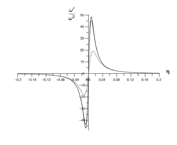
Figure 1: The non-abiabatic parameter ${\omega^{\prime}}/{\omega^{2}}$ for different values of $\xi$, with $\xi=0$ (top curve), conformal coupling $\xi=9/40$ (middle curve), and $\xi=5$ (bottom curve). As $\xi$ increases, non-adiabaticity is suppressed. Note that the non-adiabticity is concentrated near $\eta\approx 0$ for all choices of $\xi$.

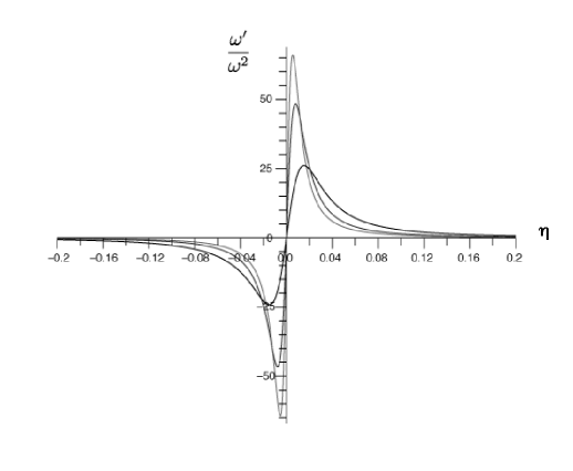
Figure 2: The non-adiabatic parameter ${\omega^{\prime}}/{\omega^{2}}$ for different values of the flux $h=1/150$ (top curve), $h=1/100$ (middle curve), and $h=1/50$ (bottom curve).

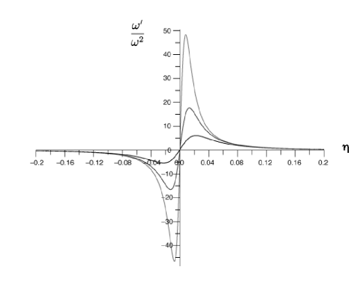
Figure 3: The non-adiabatic parameter ${\omega^{\prime}}/{\omega^{2}}$ for different values of the momentum $k_{3}=1/500$ (top line), $k_{3}=1/100$ (middle line), and $k_{3}=1/50$ (bottom line).

One point of concern is the effect of the time-dependent geometry on the effective mass

$$m^{2}_{total}=m_{eff}^{2}+\xi R+\text{gravity terms}$$

through the last three terms in (57). As seen in Fig. 1, the terms including the coupling to the geometry $\xi$, have the effect of suppressing the amount of production, but this suppression is negligible for reasonable values of the coupling. In particular, the cases of minimal ($\xi=0$) and conformal $(\xi=9/40)$ coupling have little or no effect. This can be understood by examining the Ricci curvature which, for small flux, is negligible away from the singular region (i.e., $R\sim h^{2}$). The requirement of small flux can be seen from Fig. 2, where we find that production will be suppressed unless $h<m_{p}$. Fig. 3 shows a similar result for the momenta, $k_{3}<m_{p}$. Let us now consider the production from a more quantitative perspective.

We have seen that the non-adiabaticity is focused near $\eta\approx 0$. Using this and the effective mass (48), we can expand the frequency (57) for small $\eta$

$$\omega_{k}^{2}(\eta)=f_{0}+f_{1}\eta+f_{2}\eta^{2},$$ (58)

where, after restoring the explicit dependence on $m_{p}$ ,

$$\displaystyle f_{0} = \frac{k_{3}^{2}+a_{0}m_{p}^{2}+\frac{1}{2}h^{2}}{h^{2}},\;\;\;\;\;\;\;f_{1}=\frac{a_{1}k_{3}^{2}+a_{2}m_{p}^{2}}{h^{2}},\;\;\;\;\;\;\;f_{2}=\frac{a_{3}k_{3}^{2}+a_{4}m_{p}^{2}+\frac{1}{4}h^{2}}{h^{2}},$$

$$a_{0} = (w_{0}-l_{11})^{2},\;\;\;\;a_{1}=\frac{1+3q^{2}}{3q},\;\;\;\;a_{2}=\frac{2w_{0}(w_{0}-l_{11})+3q^{2}(w_{0}^{2}-4w_{0}l_{11}+3l_{11}^{2})}{3q}$$

$$a_{3} = \frac{1+24q^{2}+9q^{4}}{18q^{2}},\;\;a_{4}=\frac{2w(w-l)+3q^{2}(13w^{2}-23wl+6l^{2})+q^{4}(9w^{2}-72wl+91l^{2})}{18q^{2}}.$$

Following the method outlined in Section IV.2, we proceed by finding the zeros of (58). The frequency vanishes at

$$\eta^{*}=\frac{-f_{1}\pm\sqrt{f_{1}^{\,2}-4\,f_{0}\,f_{2}}}{2f_{2}}.$$ (59)

Remembering that we are interested in the zeros in the lower half plane, we choose

$$\eta^{\star}=-\frac{f_{1}}{2f_{2}}-i\frac{\sqrt{4f_{0}f_{2}-f_{1}^{2}}}{2f_{2}}\equiv r-i\mu,$$ (60)

where we have $4f_{0}f_{2}-f_{1}^{2}>0$. The amount of particle production for a given mode is then given by (56), and is found to be

$$|\beta_{k}|^{2}=\biggr{(}\frac{\pi}{3}\biggr{)}^{2}e^{-\pi\frac{4f_{0}f_{2}-f_{1}^{2}}{4\,f_{2}^{3/2}}}.$$ (61)

Moreover, using the fact that $m_{p}\gg k_{3},h$, we find

$$|\beta_{k}|^{2}=\biggr{(}\frac{\pi}{3}\biggr{)}^{2}e^{-\frac{A_{1}\,m_{p}}{h}}e^{-\frac{A_{2}\,k_{3}^{2}+A_{3}\,h^{2}}{m_{p}h}+{\cal O}(\frac{1}{m_{p}^{2}})},$$ (62)

where $A_{1},A_{2},A_{3}$ are constants that depend on $w_{0},l_{11},q$.

Given this expression we can now return to the initial concern that string and membrane particle production should suffer Planck scale suppression at low energies. This can be seen by the suppression factor $e^{-\frac{A_{1}\,m_{p}}{h}}$ appearing in (62), which is related to the usual suppression due to the Hagedorn density of states (see e.g. Gubser:2003vk ). However, in this case we find that $A_{1}\propto(l_{11}-w_{0})^{3}$, which vanishes when $l_{11}=w_{0}$, consistent with the condition for having massless states at the self-dual radius $D=0$. Thus, the enhanced symmetry results in additional light states which will be copiously produced. In fact, we find significant particle production when $l_{11}=w_{0}$, given by

$$|\beta_{k}|^{2}=\biggr{(}\frac{\pi}{3}\biggr{)}^{2}e^{-\frac{3\pi}{2\,m_{p}\,h}\bigl{(}\frac{h^{2}+2k_{3}^{2}}{l_{11}\gamma}\bigr{)}},$$ (63)

where $\gamma\equiv\frac{1-3q^{2}}{q}$. Furthermore, we will choose $l_{11}=w_{0}=1$, since states with higher winding and momentum numbers would decay to this configuration. We can immediately see from (63) the same behavior that we found for the non-adiabatic parameter in the previous section. Namely, we see that for $h,k_{3}<m_{p}$ production will result and above the Planck scale production will cease. This behavior agrees with the numerical studies of the non-adiabatic parameter, which can be seen in Fig. 2 and Fig. 3.

From (63) we can calculate the eleven-dimensional number density at the creation time $\eta^{*}$ by summing over all modes

$$n_{\chi}(\eta^{*})=\frac{1}{V_{0}^{(7)}}\int_{0}^{\infty}\frac{d^{3}k_{3}}{(2\pi)^{3}}\;|\beta_{k}|^{2},$$ (64)

$V_{0}^{(7)}$ is the dimensionful volume of the extra dimensions at the time the particles were produced . The energy density of created particles is given by

$$\rho=\frac{1}{V_{0}^{(7)}}\int_{0}^{\infty}\frac{d^{3}k_{3}}{(2\pi)^{3}}\;\omega_{k}|\beta_{k}|^{2}.$$ (65)

Finally, the pressure can be found from the energy density as in (42), and the effective stress energy tensor of the produced membrane states is then

$$T^{M}_{\;\;N}=diag\left(-\rho,p_{3},p_{6},p_{11}\right).$$ (66)

V Cosmology, Backreaction, and Moduli trapping

We now want to consider the effect of the states produced in the last section on the evolution of the background (IV.1). One possible way to include the effects of such states would be to study the evolution of linear perturbations about the background (IV.1). However, one finds that this approach is not adequate, since the presence of the states alters the evolution drastically, making the effect of order one. Instead, we consider the new metric

$$ds^{2}=-dt^{2}+a(t)^{2}dx_{3}^{2}+b(t)^{2}dx_{6}^{2}+R_{11}^{2}(t)dx_{11}^{2},$$ (67)

where we will work in synchronous gauge, and we have assumed that the perturbed metric will respect the symmetries (topology) of the original metric. Introducing the Hubble parameters $H_{3}=\frac{\dot{a}}{a},H_{6}=\frac{\dot{b}}{b}$ and $H_{11}=\frac{\dot{R}_{11}}{R_{11}}$, the equations of motion can be written as

$$\dot{H}_{i}=H_{i}\sum_{j}H_{j}+8\pi G_{11}\left(p_{i}+\frac{1}{10}\left(\rho-\sum_{j}p_{j}\right)\right),$$ (68)

with $i,j=1\ldots 9,11$ running over all spatial dimensions. We have again taken the matter sources to be in the form of a perfect fluid characterized by their energy density and pressures, and having a stress tensor given by

$$T_{MN}=diag\left(\rho,a^{2}p_{3},b^{2}p_{6},R_{11}^{2}p_{11}\right).$$ (69)

The constraint equation

$$\sum_{i<j}H_{i}H_{j}=8\pi G_{11}\rho$$ (70)

and the equations motion allow one to obtain the continuity equation

$$\dot{\rho}=-\sum_{i}\left(\rho+p_{i}\right)H_{i}.$$ (71)

In general these equations are very difficult to solve. However, in the absence of matter (i.e., $\rho=p_{i}=0$) one finds the well-known Kasner solutions,

$$\displaystyle a(t)\sim t^{c_{1}},\;\;\;\;\;\;b(t)\sim t^{c_{2}},\;\;\;\;\;\;\;R_{11}(t)\sim t^{c_{3}},$$

$$\text{with}\;\;\;\sum_{i}c_{i}=\sum_{i}(c_{i})^{2}=1.$$ (72)

Thus, in a universe initially filled with radiation or matter the expansion will dilute the sources, and we expect the late-time behavior to approach that of the Kasner solution.

We want to include the effect of the produced states on the background (IV.1). As we found in the last section we can include the states through their energy density (65). It is important to note that number density is only well defined in the adiabatic out region. That is, near the region of non-adiabaticity, particle number (and thus energy density) can fluctuate. However, following Kofman:2004yc we will assume that after the first pass through the production point no further production occurs, and the particle number remains fixed. This approximation is certainly acceptable, since the exact treatment would merely increase the number of particles, enhancing the trapping mechanism we will discuss.

Perhaps a more serious drawback is the validity of the SUGRA approximation near the production point. For the background we have considered, production will occur near the Planck scale at the center of the M-theory moduli space. From the ten-dimensional point of view, this will be a fixed point of S-duality where a perturbative description of the theory is not available at this time. However, we can trust our equations away from the non-adiabatic region, and we are primarily interested in the attractive behavior towards this region. Thus, we will consider the effects coming from production, remembering that further corrections may become important near the non-adiabatic region. In the worst case, we will see that the corrections we consider lead us naturally to the non-adiabatic region, where a further knowledge of M-theory dynamics is needed.

Using the expression (63) in (64) we find for the number density at the time of creation $\eta^{*}$

$$\displaystyle n_{\chi}(\eta^{*}) = \frac{1}{V_{0}^{(7)}}\int_{0}^{\infty}\frac{d^{3}k}{(2\pi)^{3}}\;\left(\frac{\pi}{3}\right)^{2}e^{-\frac{3\pi}{h\gamma m_{p}}\left(k_{3}^{2}+\frac{1}{2}h^{2}\right)}$$ (73)

$$= \frac{\sqrt{3}\gamma^{3/2}}{648\,\pi}\left(m_{p}\,h\right)^{5}e^{-\frac{3\pi h}{2\gamma m_{p}}},$$ (74)

where we used $V_{0}^{(7)}=(h\,m_{p})^{-7/2}$. This is the number density of particles resulting from production at the time when the scale factors pass near the region of non-adiabaticity $D=C=0$. In terms of the new metric (67) the creation time will be denoted by $t_{0}$, and the production point corresponds to $R_{11}=b=1$. Away from the non-adiabatic region the number of particles will remain constant, and the density in the new metric is given by

$$n_{\chi}(t)=\left(\frac{a^{3}(t_{0})\,b^{6}(t_{0})\,R_{11}(t_{0})}{a^{3}(t)\,b^{6}(t)\,R_{11}(t)}\right)n_{\chi}(t_{0})\equiv\frac{V(t_{0})}{V(t)}n_{\chi}(t_{0}).$$ (75)

At this point it is convenient to return to setting $m_{p}=1$; we will reinstate the explicit dependence on the Planck mass when necessary. The energy density at time $t_{0}$ is given by

$$\rho(t_{0})=\frac{\pi^{2}}{9V_{0}^{(7)}}\int_{0}^{\infty}\frac{d^{3}k}{(2\pi)^{3}}\;\omega_{k}\,e^{-\frac{3\pi}{h\gamma}\left(k_{3}^{2}+\frac{1}{2}h^{2}\right)}.$$ (76)

The frequency $\omega_{k}$ evaluated in the new background takes the form

$$\omega_{k}^{2}\sim\frac{k_{3}^{2}}{a^{2}}+\left(\frac{1}{R_{11}}-R_{11}b\right)^{2}\equiv\frac{k_{3}^{2}}{a^{2}}+m_{eff}^{2},$$ (77)

where we have dropped gravitational terms which have been shown to be of higher adiabatic order and are negligible (recall that these terms scale like $h^{2}$, and $h^{2}\ll m_{eff}^{2}$). Using this frequency we find that the energy density at $t_{0}$ is given by

$$\rho(t_{0})=\frac{\pi^{2}}{9V_{0}^{(7)}}\int_{0}^{\infty}\frac{d^{3}k}{(2\pi)^{3}}\sqrt{\frac{k_{3}^{2}}{a^{2}}+m_{eff}^{2}}\;e^{-\frac{3\pi}{h\gamma}\left(k_{3}^{2}+\frac{1}{2}h^{2}\right)}.$$ (78)

At a later time $t$, the energy density scales in the same way as the number density,

$$\rho(t)=\frac{V(t_{0})}{V(t)}\frac{a\,\gamma\,h^{9/2}}{144\pi}\;m_{eff}^{2}\;e^{-\frac{3\pi}{2\gamma}\left(h-a^{2}h^{-1}m_{eff}^{2}\right)}\mathcal{K}_{1}\left(a^{2}h^{-1}m_{eff}^{2}\right),$$ (79)

where $\mathcal{K}_{1}$ is a Bessel function of the second kind.

V.1 Cosmological Evolution and Trapping

We are interested in the dynamics after passing through the ESP at $R_{11}=b=1$. Notice that in the absence of matter the background solution (IV.1) predicts that the radii (moduli) will continue to evolve to larger values. We will demonstrate that, by including the states produced at the ESP via their stress energy tensor (66), the motion of the radii will be reversed back towards the ESP, and the moduli can eventually become trapped. We again note that there should also be a contribution to the stress tensor coming from the flux, but such terms scale as $\rho\sim p_{i}\sim\frac{h^{2}}{a^{6}}$ and are therefore only important at early times (i.e. they are red-shifted by the expansion of $a(t)$).

The evolution begins in the adiabatic region, where $R_{11}>1$, $b>1$ and the mass term dominates the energy. In this limit the energy density (79) becomes

$$\rho\approx m_{eff}\,n_{\chi}(t).$$ (80)

In the opposite limit, near $R,b\approx 1$, the mass is negligible and the energy density becomes

$$\rho\approx\frac{n_{\chi}(t)}{a}.$$ (81)

From (80) we can determine the pressure in the respective dimensions using (42). We find that for $R_{11}>1$ and $b>1$ these scale as

$$\displaystyle p_{\,3} \approx 0,\;\;\;\;\;p_{\,6}\approx-\frac{n_{\chi}(t)}{6}R_{11}b,\;\;\;\;\;\;p_{\,11}\approx-n_{\chi}(t)R_{11}b\;\;\;\;\;\;\;\;\left(R_{11}>1\;\text{and}\;b>1\right).$$ (82)

We see that for large $R_{11}$ (or large $b$), the negative pressure due to the wrapped M2 branes dominates. From the equations of motion (68) we see that as $R_{11}$ grows large the negative source terms will dominate over the first terms on the right side of (68), given that $H_{11}$ is not too large. At the turning point $H_{11}=0$ and we find that $\dot{H}_{11}<0$, due to the large negative pressure $p_{11}$, showing that $R_{11}$ reaches a maximum value and turns back toward the ESP . After the radii pass through the ESP for a second time, we have $R_{11}<1$, and the pressures are then given by

$$\displaystyle p_{\,3} \approx 0,\;\;\;\;\;\;\;p_{\,6}\approx\frac{n_{\chi}(t)}{6}R_{11}b,\;\;\;\;\;\;\;p_{\,11}\approx\frac{n_{\chi}(t)}{R_{11}}\;\;\;\;\;\;\;\;\;\;\;\;\;\;\;\left(R_{11}<1\right),$$ (83)

In the last step we have assumed that the radii have moved sufficiently below the ESP so that we are again in an adiabatic region, and (80) still gives the relevant energy density. We see from (83) that as $R_{11}$ continues to evolve towards smaller values, the pressure becomes large and positive. From (68) this means that $R_{11}$ will reach a minimum value and go back towards the ESP. This behavior will continue and $R_{11}$ will oscillate around the ESP, with the oscillations damping due to the expansion of $a(t)$.

However, one place we have been cavalier is in the evolution of the extra dimensional scale factor $b$. In fact, from its associated pressure (83) we see that for $b\ll 1$ the pressure will vanish. Thus, since there is no pressure to prevent its collapse, $b$ will continue to run to smaller values. Furthermore, we have over-simplified the entire evolution by assuming that $R_{11}=1$ and $b=1$ occur simultaneously. If this were the case it would be the result of extreme fine-tuning.

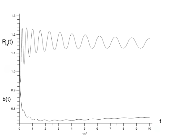
Figure 4: Evolution of $R_{11}$ and $b$ for the exact density (79) and pressures, including only the membrane sources related to $R_{11}$.

Instead, as can be seen in Fig. 4, we find that for differing values of $R_{11}$ and $b$ trapping of $R_{11}$ can occur away from the ESP at a value that is determined by the running of $b$ to its asymptotic value.

Despite the evolution of $b$, we can remedy the situation by simply including the other membrane states discussed in Section II. That is, near $b=1/\sqrt{R_{11}}$ there are additional massless states that can be produced with masses

$$m^{(b)}_{eff}=\left|\frac{1}{b}-R_{11}(t)b(t)\right|,$$ (84)

where now the momentum is taken in the $b$ direction (i.e., $k_{9}\neq 0$, $k_{11}=0$). The production of these states is handled analogously to the previous states, and leads to an additional contribution to the energy density

$$\rho^{(b)}=6\,\tilde{n}_{\chi}(t)\,m_{eff},$$ (85)

where the factor of six comes from considering states produced equally in all six dimensions. These states provide the needed pressure term at small $b$

$$\displaystyle p^{(b)}_{6} = \frac{\tilde{n}_{\chi}(t)}{b}\;\;\;\;\;\;\;\;\;\;\;\;\;\;\;\;\;\;\;\;\left(b<1\right),$$ (86)

which will cause the motion of $b$ to return to the ESP.

Given the additional sources, we now expect from the asymptotic behavior that the moduli should be trapped. However, the dynamics is actually quite involved due to the presence of non-linearities. Using the experimental result that $H_{3}>0$ (i.e. we live in three large dimensions), we examine the system numerically with the results appearing in Figures 5 $-$ 7. In Fig. 5, we see the evolution of the radii $R_{11}$ and $b$ given initial conditions consistent with $H_{3}>0$.

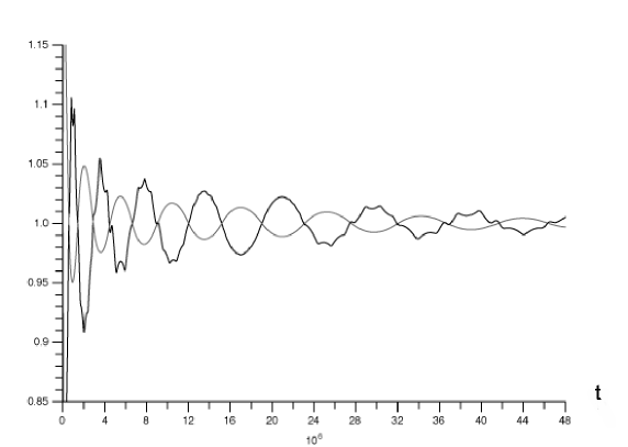
Figure 5: Evolution of $R_{11}$ (dark curve) and $b$ (light curve) for the exact density (79) and pressures, including membranes in all extra dimensions.

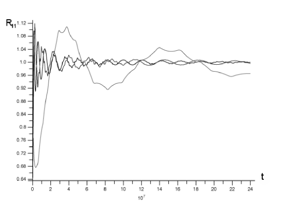
Figure 6: $R_{11}$ for differing initial values of the expansion rate, with $\dot{R}_{0}=(0.001,0.5)$ being barely distinguishable and with $\dot{R}_{0}=0.6$ (light curve) we see the period begins to grow. We see that as the initial expansion rate is increased trapping takes longer to occur with $H_{11}>m_{p}$ leading to the case of no trapping.

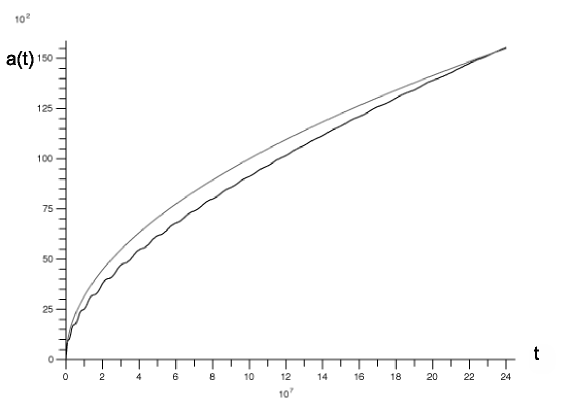
Figure 7: Evolution of $a(t)$ compared to $t^{1/2}$.

The jagged oscillations along the curve of $R_{11}$ are not due to numerical error, but rather result from the coupling to $b$ and the discontinuities associated with the pressure changing sign. We find that the radii will continue to oscillate with a decreasing amplitude, due to the expansion of $a(t)$. At late times we find that the radii $R_{11}$ and $b$ approach a constant value, which from (81) implies $\rho\sim a^{-4}$ and $a(t)\sim t^{1/2}$. That is, our three dimensional universe evolves to that of a radiation dominated universe and the radii are trapped near the ESP $R_{11}=b=1$. We find that the trapping is robust, given that the initial expansion rates of the radii do not exceed the Planck scale (i.e., $H_{6}<m_{p}$ and $H_{11}<m_{p}$. This condition can be seen from Fig. 6, where we have plotted the evolution of $R_{11}$ for increasing values of the initial expansion rate $H_{11}$, and a similar result follows for $b(t)$. In Fig. 7 we have presented a comparison of the late time behavior of $a(t)$ versus that of a radiation dominated universe $a(t)\sim t^{1/2}$. The wiggles in the evolution of $a(t)$ before the radii completely stabilize, naively may suggest the possibility of cosmological signatures coming from the trapping mechanism.

VI Conclusions and Future Prospects

We have considered both classical and quantum corrections to low-energy M-theory coming from dynamics of BPS membrane bound states whose effective mass depends on the radii of the extra dimensions. Including such states classically leads to an attractor mechanism that fixes moduli but is inconsistent with the use of the effective field theory approach.

Insisting on an effective field theory description, we then consider quantum mechanical production of these membranes in a time-dependent background, and find the expected result that the production suffers Planckian suppression. However, we do find the possibility of significant and finite production for states that exhibit enhanced symmetry. We believe that these should correspond to non-threshold bound states of membranes and gravitational waves, which become tensionless at the eleven-dimensional self-dual point, $R_{11}=l_{p}$. An exact construction of such states is challenging, due to the problems of quantizing the supermembrane and the lack of an effective description of the theory in this regime.

In Russo:1996if it was shown that one can obtain the BPS spectrum of the supermembrane in special limits and by utilizing properties of BPS configurations. However, the enhanced states we are interested in require non-vanishing vacuum energy, which is not compatible with the $\mathcal{N}=2$ SUSY case considered in Russo:1996if . Therefore, guided by the analysis of Russo:1996if , we conjecture the existence of the enhanced states, awaiting a more concrete construction. One possibility for their existence is the case of $\mathcal{N}=1$ heterotic M-theory, in analogy with the enhanced gauge symmetry of heterotic strings. Another intriguing possibility is the recent conjecture that the spectrum of string / M-theory contains states that lie below the BPS bound Arkani-Hamed:2006dz .

Assuming that such enhanced states exist, we find that they can have a critical impact on the evolution of moduli, which would have been missed in the naive low-energy effective theory neglecting dynamics. We have found that, by including the backreaction of the membrane states produced, the radii are dynamically attracted to values near fixed points of S- and T- duality. This effect would be missed if one did not have a knowledge of (enhanced) M-theory states having masses which depend on evolving moduli. Thus, the lesson we learn is that the presence of time-dependence introduces a dynamical mass scale that must be taken into careful consideration in the effective field theory. Furthermore, it is paramount not to forget the string theory origin of the low-energy effective action.

In addition to the corrections from on-shell particle production which we have explored here, there will be radiative corrections coming from the presence of the light membrane states. In fact, it was shown in Silverstein:2003hf that, for the case of colliding D-branes, open strings becoming light lead to corrections to the gauge theory propagator resulting in a speed limit for the moduli. In the case we have considered here a similar story should hold, but this time it is the closed string moduli which should be slowing down (the radii of the extra dimensions). This offers a challenge, since the gauge theory interpretation of such processes is unclear. We find the possibility of speed limits for radii intriguing, and we hope to report on it shortly.

- (1) C. Vafa, “The string landscape and the swampland,” arXiv:hep-th/0509212.
- (2) N. Arkani-Hamed, L. Motl, A. Nicolis and C. Vafa, “The string landscape, black holes and gravity as the weakest force,” arXiv:hep-th/0601001.
- (3) E. Silverstein and D. Tong, “Scalar speed limits and cosmology: Acceleration from D-cceleration,” Phys. Rev. D 70, 103505 (2004) [arXiv:hep-th/0310221].
- (4) L. Kofman, A. Linde, X. Liu, A. Maloney, L. McAllister and E. Silverstein, “Beauty is attractive: Moduli trapping at enhanced symmetry points,” JHEP 0405, 030 (2004) [arXiv:hep-th/0403001].
- (5) S. Watson, “Moduli stabilization with the string Higgs effect,” Phys. Rev. D 70, 066005 (2004) [arXiv:hep-th/0404177].
- (6) M. Alishahiha, E. Silverstein and D. Tong, “DBI in the sky,” Phys. Rev. D 70, 123505 (2004) [arXiv:hep-th/0404084].
- (7) R. Brustein, S. P. de Alwis and E. G. Novak, “M-theory moduli space and cosmology,” Phys. Rev. D 68, 043507 (2003) [arXiv:hep-th/0212344].
- (8) M. Dine, Y. Nir and Y. Shadmi, “Enhanced symmetries and the ground state of string theory,” Phys. Lett. B 438, 61 (1998) [arXiv:hep-th/9806124].
- (9) J. G. Russo and A. A. Tseytlin, “Waves, boosted branes and BPS states in M-theory,” Nucl. Phys. B 490, 121 (1997) [arXiv:hep-th/9611047].
- (10) J. H. Schwarz, “Superstring dualities,” Nucl. Phys. Proc. Suppl. 49, 183 (1996) [arXiv:hep-th/9509148].
- (11) J. H. Schwarz, “Lectures on superstring and M theory dualities,” Nucl. Phys. Proc. Suppl. 55B, 1 (1997) [arXiv:hep-th/9607201].
- (12) E. Bergshoeff, E. Sezgin and P. K. Townsend, “Properties Of The Eleven-Dimensional Super Membrane Theory,” Annals Phys. 185, 330 (1988).
- (13) M. J. Duff, T. Inami, C. N. Pope, E. Sezgin and K. S. Stelle, “Semiclassical Quantization Of The Supermembrane,” Nucl. Phys. B 297, 515 (1988).
- (14) J. G. Russo, “Supermembrane dynamics from multiple interacting strings,” Nucl. Phys. B 492, 205 (1997) [arXiv:hep-th/9610018].
- (15) J. J. Friess, S. S. Gubser and I. Mitra, “String creation in cosmologies with a varying dilaton,” Nucl. Phys. B 689, 243 (2004) [arXiv:hep-th/0402156].
- (16) T. Battefeld and S. Watson, “String gas cosmology,” arXiv:hep-th/0510022.
- (17) R. H. Brandenberger, “Challenges for string gas cosmology,” arXiv:hep-th/0509099.
- (18) R. H. Brandenberger, “Moduli stabilization in string gas cosmology,” arXiv:hep-th/0509159.
- (19) S. P. Patil, “Moduli (dilaton, volume and shape) stabilization via massless F and D string modes,” arXiv:hep-th/0504145.
- (20) N. Kaloper, J. Rahmfeld and L. Sorbo, “Moduli entrapment with primordial black holes,” Phys. Lett. B 606, 234 (2005) [arXiv:hep-th/0409226].
- (21) S. A. Abel and J. Gray, “On the chaos of D-brane phase transitions,” JHEP 0511, 018 (2005) [arXiv:hep-th/0504170].
- (22) T. Mohaupt and F. Saueressig, “Conifold cosmologies in IIA string theory,” Fortsch. Phys. 53, 522 (2005) [arXiv:hep-th/0501164].
- (23) A. Berndsen, T. Biswas and J. M. Cline, “Moduli stabilization in brane gas cosmology with superpotentials,” JCAP 0508, 012 (2005) [arXiv:hep-th/0505151].
- (24) A. Strominger, “Massless black holes and conifolds in string theory,” Nucl. Phys. B 451, 96 (1995) [arXiv:hep-th/9504090].
- (25) J. E. Lidsey, D. Wands and E. J. Copeland, “Superstring cosmology,” Phys. Rept. 337, 343 (2000) [arXiv:hep-th/9909061].
- (26) A. E. Lawrence and E. J. Martinec, “String field theory in curved spacetime and the resolution of spacelike singularities,” Class. Quant. Grav. 13, 63 (1996) [arXiv:hep-th/9509149].
- (27) S. S. Gubser, “String production at the level of effective field theory,” Phys. Rev. D 69, 123507 (2004) [arXiv:hep-th/0305099].
- (28) N. D. Birrell and P. C. W. Davies, “Quantum Fields In Curved Space,”
- (29) D. J. H. Chung, “Classical inflation field induced creation of superheavy dark matter,” Phys. Rev. D 67, 083514 (2003) [arXiv:hep-ph/9809489].
- (30) S. Watson and R. Brandenberger, “Stabilization of extra dimensions at tree level,” JCAP 0311, 008 (2003) [arXiv:hep-th/0307044].