Conformal field theory description of mesoscopic phenomena in the fractional quantum Hall effect

L. GeorgievCFT description of mesoscopic phenomena in the FQH effect

1

1

We give a universal description of the mesoscopic effects occurring in fractional quantum Hall disks due to the Aharonov–Bohm flux threading the system. The analysis is based on the exact treatment of the flux within the conformal field theory framework and is relevant for all fractional quantum Hall states whose edge states CFTs are known. As an example we apply this scheme for the parafermion Hall states and extract the main characteristics of the low- and high- temperature asymptotic behavior of the persistent currents.

1 Introduction

Mesoscopic systems are characterized by their intermediate size in between the micro- and macro- systems—small enough so that the electrons still move in a coherent way, yet big enough for some measurable consequences such as the Aharonov–Bohm (AB) effect to be observable. One important property of the mesoscopic rings threaded by AB flux is that the free energy of the ring is a periodic function of the flux with period one flux quantum $h/e$ (Bloch theorem). In addition to its natural relevance for studying quantum effects mesoscopic physics has been at the core of the very promising recent proposal [1] for topological quantum computers in terms of the braid matrices of non-abelian fractional quantum Hall (FQH) anyons. The advantage of such topological gates, as compared to the other existing quantum computation schemes, is that quantum information is encoded in a non-local way which makes it inaccessible to local interactions and decoherence. In this talk we demonstrate that it is possible and very convenient to compute mesoscopic quantities such as the persistent currents for FQH rings purely from their edge states conformal field theory (CFT) by using the CFT partition function with flux. The effect of adding AB flux is simply twisting the electron and quasiparticle operators. The numerical results [2, 3] show that the period of the persistent currents for the parafermion FQH states [4, 2, 3] is exactly one flux quantum which means that there could be no spontaneous breaking of continuous symmetries. We derive an analytic formula for the low-temperature amplitudes of persistent currents which are shown to decay logarithmically due to thermal activation of q.h.–q.p. pairs. Also we find an analytic formula for the high-temperature asymptotics of the persistent currents which decay exponentially due to thermal decoherence with universal non-Fermi liquid exponent derived from the CFT. These exponents can be used to characterize unambiguously the FQH universality classes.

2 Persistent currents: an intuitive picture

When at zero temperature the AB flux, threading a FQH system in the Corbino ring geometry shown on Fig. 1, is increased adiabatically this induces azimuthal electric field $\vec{E}_{\phi}$ however there is no azimuthal bulk current since $\sigma_{xx}=0$. But because $\sigma_{H}\neq 0$ there is a radial current pulse which transfers charges between the two edges. This leads to edge currents imbalance and produces a non-zero net current.

Figure 1: Corbino ring geometry for FQH system threaded by AB flux

Despite the huge non-mesoscopic contribution [5] these oscillating mesoscopic persistent currents could be measured by two-point-contact SQUID detectors.

3 The quantum Hall effect and conformal field theory

In the classical Hall effect the conductance of a two-dimensional conducting plate in presence of normal magnetic field $B$ has a nonzero off-diagonal component $\sigma_{H}$. The quantum Hall effect is characterized by the quantized $\sigma_{H}$ and at the same time the vanishing diagonal conductance

$$\widehat{\sigma}=\left[\begin{array}[]{cc}0&-\sigma_{H}\\ \sigma_{H}&0\end{array}\right],\quad{\sigma}_{H}=\left(\frac{e^{2}}{h}\right)\nu,\quad\nu_{H}=\frac{n}{n_{B}},\quad n_{B}=\frac{B}{h/e},$$

where $n$ is the electron density and $\nu_{H}=n_{H}/d_{H}$ the filling factor. In order to observe this effect one needs high magnetic fields ($B\sim 1-30$ T), low temperature ($T<1$ K), low electric fields, low electron density ($n\sim 10^{11}\ cm^{-2}$), high mobility ($\mu\sim 10^{5}-10^{7}\ cm^{2}/V.s$) and extremely high-quality samples.

3.1 Effective quantum field theory approach: the 2+1 dimensional Chern–Simons model

The presence of the bulk energy gap in the low-energy spectrum of FQH liquid implies that it is incompressible, i.e., when the system is on a plateau of $\sigma_{H}$ changing $B$ slowly leads to low-energy (de)compression which are suppressed by the gap and therefore $\sigma_{H}$ does not change. The effective quantum field theory (QFT) for the low-energy excitations of the incompressible electron fluid has been obtained in the thermodynamic scaling limit [6, 7]—the non-relativistic interacting Schrödinger electrons plus incompressibility leads to abelian $2+1$ dimensional Chern–Simons QFT

$$S_{\mathrm{eff}}=\frac{\sigma_{H}}{2}\int a\wedge da,\quad(a_{\mu})=\frac{e}{\hbar}(A_{0},-A_{1},-A_{2}).$$

The current in response to the external electromagnetic field for a finite sample with boundaries

$$j^{\mu}=\frac{\delta S_{\mathrm{eff}}(A)}{\delta A_{\mu}}=\sigma_{H}\varepsilon^{\mu\nu\rho}\partial_{\nu}A_{\rho}\quad\Longrightarrow\quad\left\{\begin{array}[]{l}j_{0}=\sigma_{H}\,B\\ j_{k}=\sigma_{H}\,\varepsilon_{kl}\,E_{l}\end{array}\right.$$

turns out to be anomalous. This induces a current $j_{\alpha}$ along the boundaries

$$\partial_{\alpha}j^{\alpha}=\frac{1}{2}\sigma_{H}\epsilon_{\alpha\beta}F_{\alpha\beta},\quad\sigma_{H}=\frac{e^{2}}{h}\nu_{H},\quad F_{\alpha\beta}=\partial_{\alpha}A_{\beta}-\partial_{\beta}A_{\alpha},$$

which is anomalous too, however, the bulk anomaly is exactly compensated by that of the edge currents so that the total current is conserved. This bulk–edge anomaly cancellation is the origin of the so called holographic principle implying the precise correspondence between bulk and edge spectra [7].

3.2 The correspondence between Chern–Simons and RCFT

According to Witten’s correspondence the $(2+1)$ dimensional Chern–Simons QFT on the dense cylinder $(t,x)\in{\mathbb{R}}\times\mathrm{Disk}$ is equivalent to the rational $(1+1)$ dimensional CFT on the spacetime border $(t,\tilde{x})\in{\mathbb{R}}\times\mathrm{Circle}$. This correspondence is not exactly one-to-one: one bulk QFT corresponds to many boundary CFTs, however one boundary CFT corresponds to only one bulk QFT. The correlation functions of the bulk observables can be obtained from the CFT correlation functions by analytic continuation. Because the edge states dynamics determines all universal properties it is believed that the FQH universality classes can be labeled by the rational CFT (RCFT) for the edge states.

3.3 CFT description of quasiparticles

The CFT for the FQH edges always contains $\widehat{u(1)}\times Vir$ symmetry. The first factor describes the electric charge while the second one—the angular momentum. The FQH universality class can be described in terms of a single-edge chiral CFT, i.e., corresponding to disk FQH states. The quasiparticle excitations are labeled by the weights of the irreducible representations of the CFT chiral algebra [7, 8]. One of the most important characteristics of this CFT is its topological order—the number of topologically inequivalent quasiparticles whose irreducible representation spaces are closed under fusion—which in the CFT language is equal to the dimension of the modular $S$ matrix. In addition the RCFT for a FQH ring with two edges must satisfy 4 invariance conditions ($T^{2}$, $S$, $U$, $V$) [9].

The electron and the basic quasihole in the CFT are represented by the primary fields [7, 8]

$$\psi_{\mathrm{el}}(z)={\mbox{{:}}{\mathrm{e}^{-i\frac{1}{\sqrt{\nu_{H}}}\phi^{(c)}(z)}}{\textrm{:}}}\otimes\psi^{(0)}(z),\quad\psi_{\mathrm{qh}}(\eta)={\mbox{{:}}{\mathrm{e}^{i\frac{1}{\sqrt{n_{H}d_{H}}}\phi^{(c)}(\eta)}}{\textrm{:}}}\otimes\psi^{(0)}_{\mathrm{qh}}(\eta).$$

where $\psi^{(0)}(z)\in Vir$ and $\psi^{(0)}_{\mathrm{qh}}(\eta)\in Vir$ are the neutral component of the electron and the quasihole, respectively. The wave functions of $N$ electrons and $k$ quasiholes (ground state corresponds to $k=0$) are computed as chiral CFT correlation functions

$$\Psi(\eta_{1},\ldots,\eta_{k};z_{1},\ldots,z_{N})=\langle 0|\psi_{\mathrm{qh}}(\eta_{1})\cdots\psi_{\mathrm{qh}}(\eta_{k})\psi_{\mathrm{el}}(z_{1})\cdots\psi_{\mathrm{el}}(z_{N})|N,k\rangle.$$

Finally, we would like to introduce the notion of mesoscopic FQH rings. We consider a single edge FQH system on a Corbino disk. The bulk energy gap implies that all low-energy excitations are living on the edge which, under certain experimental conditions ($R\sim 5\ \mu$m, $T\sim 1$ mK) can be considered a mesoscopic ring displaying Aharonov–Bohm oscillations of the magnetization [10]. While the disk geometry is a little inconvenient for analyzing flux-threading phenomena, the chiral CFT description presented here appears very useful in antidot FQH states threaded by Aharonov–Bohm flux [11, 12].

4 Aharonov–Bohm flux: twisting the electrons

In this section we shall consider the effect of adding Aharonov–Bohm magnetic field described by the vector potential

$$\mathbf{A}=\left(\frac{h}{e}\right)\frac{\phi}{2\pi r^{2}}\,(-y,x)=\left(\frac{h}{e}\right)\frac{\phi}{2\pi r}\ \mathbf{e_{\varphi}},\quad\phi\in{\mathbb{R}}\quad\left(\mathrm{rot}\,\mathbf{A}=\phi\ \delta^{(2)}(\mathbf{r})\right)$$

where $\phi$ is the AB flux in units $\phi_{0}=h/e$, $r=\sqrt{x^{2}+y^{2}}$, to quantum Hall systems [8]. Because the AB magnetic field is zero along the edge, the electron operator in AB field could be obtained by explicit computation [8] of the line integral below

$$\psi^{A}_{\mathrm{el}}(z)=\exp\left(-i\frac{e}{\hbar}\int\limits_{*}^{z}{\bf A}.d{\bf r}\right)\ \psi_{\mathrm{el}}(z)=z^{-\phi}\ \psi_{\mathrm{el}}(z),\quad z=x+iy,$$ (1)

where $\psi_{\mathrm{el}}(z)$ is the electron in the absence of flux. This procedure is known in CFT as orbifold twisting. Note that the AB flux twists only the $\widehat{u(1)}$ part of the electron [8] which is the usual vertex exponent of a normalized $\widehat{u(1)}$ boson

$${\mbox{{:}}{\mathrm{e}^{i\alpha\phi^{(c)}(z)}}{\textrm{:}}}\ \stackrel{{\scriptstyle\mathrm{def}}}{{=}}\ U_{\alpha}\,\mathrm{e}^{i\alpha\phi^{(c)}_{+}(z)}\,z^{\alpha J_{0}}\,\mathrm{e}^{i\alpha\phi^{(c)}_{-}(z)},\quad i\phi^{(c)}_{\pm}(z)=\pm\sum_{n=1}^{\infty}J_{\mp n}\frac{z^{\pm n}}{n},$$

where $U_{\alpha}$ are the (outer) charge-shift automorphisms of the $\widehat{u(1)}$ current algebra generated by the Laurent modes of the current $J(z)=i\,\partial\phi^{(c)}(z)=\sum_{n\in{\mathbb{Z}}}J_{n}z^{-n-1}$ with commutation relations $\left[J_{n},J_{m}\right]=n\,\delta_{n+m,0}$, i.e.,

$$\left[J_{n},U_{\alpha}\right]=\alpha\,U_{\alpha}\,\delta_{n,0},\quad U_{\alpha}\,U_{\beta}=U_{\alpha+\beta},\quad\alpha,\beta\in{\mathbb{R}},\quad U_{0}=1,\quad\left(U_{\alpha}\right)^{\dagger}=U_{-\alpha}.$$

Comparing the twisting results [13] for a general twist $\pi_{\beta}\ :\ A\to U_{\beta}\,A\,U_{-\beta}$

$${\mbox{{:}}{\mathrm{e}^{i\alpha\phi^{(c)}(z)}}{\textrm{:}}}\quad\stackrel{{\scriptstyle\pi_{\beta}}}{{\longrightarrow}}\quad U_{\beta}\,{\mbox{{:}}{\mathrm{e}^{i\alpha\phi^{(c)}(z)}}{\textrm{:}}}\,U_{-\beta}=z^{-\alpha\beta}\,{\mbox{{:}}{\mathrm{e}^{i\alpha\phi^{(c)}(z)}}{\textrm{:}}},$$

where $\alpha=-1/\sqrt{\nu_{H}}$ for the electron, with $\nu_{H}$ the filling factor, to Eq. (1) we find that the twist $\beta$ is proportional to the AB flux $\phi$

$$-\left(\frac{-1}{\sqrt{\nu_{H}}}\right)\,\beta=-\phi\quad\Longrightarrow\quad\beta\equiv-\sqrt{\nu_{H}}\,\phi.$$

The electric $\widehat{u(1)}$ current $J^{\mathrm{el}}(z)=i\sqrt{\nu_{H}}\,\partial\phi^{(c)}(z)=\sum_{n\in{\mathbb{Z}}}J^{\mathrm{el}}_{n}\ z^{-n-1}$ becomes twisted as well [13]

$$J^{\mathrm{el}}(z)\quad\stackrel{{\scriptstyle\pi_{\beta}}}{{\longrightarrow}}\quad J^{\mathrm{el}}(z)+\frac{\nu_{H}\phi}{z}\qquad\Longleftrightarrow\qquad J^{\mathrm{el}}_{n}\quad\stackrel{{\scriptstyle\pi_{\beta}}}{{\longrightarrow}}\quad J^{\mathrm{el}}_{n}+\nu_{H}\phi\ \delta_{n,0}.$$ (2)

so that the $\widehat{u(1)}$ part of the (Sugawara) stress tensor $T^{(c)}(z)=(1/2){\mbox{{:}}{J(z)^{2}}{\textrm{:}}}$ is twisted too

$$L_{n}^{(c)}\ \stackrel{{\scriptstyle\pi_{\beta}}}{{\longrightarrow}}\ L_{n}^{(c)}+\phi J^{\mathrm{el}}_{n}+\nu_{H}{\phi^{2}\over 2}\delta_{n,0}.$$

Thus the total stress tensor $T(z)=T^{(c)}(z)+T^{(0)}(z)=\sum_{n}\ L_{n}\ z^{-n-2}$ is modified by the AB flux [8] as follows

$$L_{n}=L_{n}^{(c)}+L_{n}^{(0)},\qquad\qquad L_{n}\ \stackrel{{\scriptstyle\pi_{\beta}}}{{\longrightarrow}}\ L_{n}+\phi J^{\mathrm{el}}_{n}+\nu_{H}\frac{\phi^{2}}{2}\delta_{n,0}.$$ (3)

The chiral CFT partition function which we shall use as a thermodynamic potential for $T\geq 0$ is computed as the trace of the Boltzmann factor over the Hilbert space, ${\mathcal{H}}=\mathop{\oplus}_{\lambda=1}^{N}{\mathcal{H}}_{\lambda}$, containing all superselection sectors corresponding to all kind of static topologically inequivalent point-like sources within the disk,

$$Z(\tau,\zeta)=\mathop{\mathrm{tr}}_{\quad{\mathcal{H}}\ }\mathrm{e}^{2\pi i\left[\tau\left(L_{0}-\frac{c}{24}\right)+\zeta J_{0}^{\mathrm{el}}\right]}=\sum_{\lambda=1}^{N}\chi_{\lambda}(\tau,\zeta),$$

Now that we know the expressions for the stress tensor (3) and electric current (2) in presence of AB flux we can compute the total chiral CFT partition function in presence of AB flux $\phi$

$$Z_{\phi}(\tau,\zeta) = \mathop{\mathrm{tr}}_{\quad{\mathcal{H}}\ }\mathrm{e}^{2\pi i\left[\tau\left(L_{0}+\phi J_{0}^{\mathrm{el}}+\nu_{H}\frac{\phi^{2}}{2}-\frac{c}{24}\right)+\zeta\left(J_{0}^{\mathrm{el}}+\nu_{H}\phi\right)\right]}$$ (4)

$$= \mathrm{e}^{2\pi i\nu_{H}\left[\frac{\phi^{2}}{2}\tau+\phi\zeta\right]}\ Z(\tau,\zeta+\phi\tau).$$

Equation (4) is our main result in this section: adding AB flux $\phi$ essentially amounts to shifting the modular parameter $\zeta\to\zeta+\phi\tau$. The precise thermodynamical identification of the modular parameters, which for a chiral sample (single circular edge of circumference $L$ and edge velocity $v_{F}$) have to be pure imaginary, with the absolute temperature $T$ and AB flux $\phi$ is [8]

$$q=\mathrm{e}^{2\pi i\tau},\quad\tau=i\pi\frac{T_{0}}{T},\quad\zeta=\phi\tau,\quad T_{0}=\frac{\hbar v_{F}}{\pi k_{B}L},\quad\phi\in{\mathbb{R}}.$$

5 Persistent currents for the ${\mathbb{Z}}_{k}$ parafermion FQH states

5.1 The RCFT for the ${\mathbb{Z}}_{k}$ parafermion FQH states

The RCFT for the ${\mathbb{Z}}_{k}$ parafermion FQH states has the general $\widehat{u(1)}\times Vir$ structure emphasized in Sect. 3.3

$$\left(\widehat{u(1)}\oplus\mathrm{PF}_{k}\right)^{{\mathbb{Z}}_{k}},\quad\mathrm{PF}_{k}=\frac{\widehat{su(k)_{1}}\oplus\widehat{su(k)_{1}}}{\widehat{su(k)_{2}}}$$ (5)

where the neutral $Vir$ component of the chiral algebra is realized as a diagonal affine coset [2, 8, 14]. The FQH states corresponding to the RCFT in (5), which correspond to central charge $c=1+2(k-1)/(k+1)$ and filling factor $\nu_{k}=2+k/(k+2)$ have been introduced in [4]. The edge excitations are represented by the primary fields of (5) labeled by $(\lambda,\Phi)\Rightarrow\ :\mathrm{e}^{i\frac{\lambda}{\sqrt{k(k+2)}}\phi^{(c)}(z)}:\otimes\ \Phi(z)$, where the neutral excitation is a ${\mathbb{Z}}_{k}$ parafermion primary field $\Phi(z)\in\mathrm{PF}_{k}^{*}$. The superscript ${\mathbb{Z}}_{k}$ denotes a selection rule called the ${\mathbb{Z}}_{k}$ Pairing Rule (PR) [2, 8] which says that an excitation with label $(\lambda,\Phi)$ is allowed only if

$$P\left[\Phi\right]=\lambda\ \,\mathrm{mod}\,\ k,$$

with $P\left[\Phi\right]$ the parafermion ${\mathbb{Z}}_{k}$-charge of $\Phi$. For more details about the parafermion FQH states and the diagonal coset construction see Refs. [4, 2, 8, 14].

5.2 Partition function and persistent currents

According to the standard thermodynamic interpretation the partition function computed in the CFT is related to the free energy by $F(T,\phi)=-k_{B}T\ln Z(T,\phi)$ and its dependence on the AB flux gives rise to an equilibrium persistent current

$$I(T,\phi)=\left(\frac{e}{h}\right)\,k_{B}T\frac{\partial}{\partial\phi}\ln Z(\tau,\phi\tau).$$

The total chiral partition function for the ${\mathbb{Z}}_{k}$ parafermion states is

$$Z_{k}(\tau,\zeta)=\mathrm{e}^{-{\pi}\nu_{H}\frac{\left(\mathrm{Im}\ \zeta\right)^{2}}{\mathrm{Im}\ \tau}}\sum_{l\,\mathrm{mod}\,k+2}\quad\sum_{\rho\geq l-\rho\,\mathrm{mod}\,k}\chi_{l,\rho}(\tau,\zeta),$$

where the characters of the RCFT (5) are expressed in terms of the $\widehat{u(1)}$ characters $K_{l}(\tau,k\zeta;k(k+2))$ and those, $\mathrm{ch}\left(\underline{\Lambda}_{l-\rho+s}+\underline{\Lambda}_{\rho+s}\right)(\tau)$, for the parafermions

$$\chi_{l,\rho}(\tau,\zeta)=\sum_{s=0}^{k-1}K_{l+s(k+2)}(\tau,k\zeta;k(k+2))\mathrm{ch}\left(\underline{\Lambda}_{l-\rho+s}+\underline{\Lambda}_{\rho+s}\right)(\tau),$$

whose explicit forms can be found in Refs. [2, 8, 14].

5.3 Low temperature regime: $T\ll T_{0}$

Because in the low-temperature limit $T\to 0$ the modular parameter $q=\exp\left(-2\pi^{2}\frac{T_{0}}{T}\right)\to 0$ we can keep only the leading terms in $Z(\tau,\zeta)$ which come from the RCFT sectors with lowest CFT-dimensions only, i.e., the vacuum and the one-quasiparticle and one-quasihole sectors

$$Z(T,\phi)\mathop{\simeq}\limits_{\ T\ll T_{0}\ }q^{\frac{\nu_{H}}{2}\phi^{2}}\left\{1+q^{\Delta_{\mathrm{qh}}}\left(q^{Q_{\mathrm{qh}}\phi}+q^{-Q_{\mathrm{qh}}\phi}\right)\right\},\quad Q_{\mathrm{qh}}=\frac{1}{k+2},$$

from which we obtain the low-T asymptotics of persistent current amplitude

$$I_{\max}(T)\ \mathop{\simeq}\limits_{T\ll T_{0}}\ \nu_{H}\frac{ev_{F}}{L}\left\{\frac{1}{2}-\frac{k_{B}T}{2\widetilde{\varepsilon}_{\mathrm{qh}}}\left[1+\ln\left(\frac{1}{n_{H}}\frac{2\widetilde{\varepsilon}_{\mathrm{qh}}}{k_{B}T}\right)\right]\right\},$$ (6)

where $\widetilde{\varepsilon}_{\mathrm{qh}}$ is the proper quasihole energy [3, 8]

$$\widetilde{\varepsilon}_{\mathrm{qh}}=2\pi^{2}k_{B}T_{0}\ \Delta_{\mathrm{qh}},\qquad\Delta_{\mathrm{qh}}=\frac{1}{2n_{H}d_{H}}+\Delta^{(0)}_{\mathrm{qh}},\qquad\Delta^{(0)}_{\mathrm{qh}}=\frac{k-1}{2k(k+2)}.$$

The low-temperature logarithmic decay of the persistent currents amplitudes (6) can be interpreted as due to thermal activation of quasiparticle–quasihole pairs. Note that the fundamental quasiholes in the parafermion FQH states have the lowest electric charge $1/(k+2)$ and CFT dimension $1/(2k+4)$.

5.4 High temperature regime: $T\gg T_{0}$

At very high temperatures the modular parameter $q=\exp\left(-2\pi^{2}\frac{T_{0}}{T}\right)\to 1$ in which limit the partition function is divergent. Therefore, it is convenient to first perform a modular $S$ transformation $(\tau,\zeta)\to(-1/\tau,-\zeta/\tau)$ after which the new modular parameter $q^{\prime}=\exp(2\pi i\tau^{\prime})\to 0$ for $T\to\infty$. Now the high-temperature expansion of the partition function is determined by the leading terms, however for $q^{\prime}\to 0$ in the characters $\chi_{\lambda}(\tau^{\prime},\zeta^{\prime})$,

$$Z(\tau,\zeta)=\sum_{\lambda=1}^{N}\chi_{\lambda}(\tau^{\prime},\zeta^{\prime})\left(\sum_{\lambda^{\prime}=1}^{N}S_{\lambda\lambda^{\prime}}\right)$$

for which the $S$ matrix is explicitly needed. Using the $S$ matrix computed in [8] we obtain the following exponential decay of the persistent currents amplitudes

$$\overline{I}_{k}(T)\ \mathop{\simeq}_{T\gg T_{0}}\ I^{0}_{k}\left(\frac{T}{T_{0}}\right)\exp\left(-\alpha_{k}\frac{T}{T_{0}}\right),\quad I^{0}_{k}=\mathrm{const.}$$

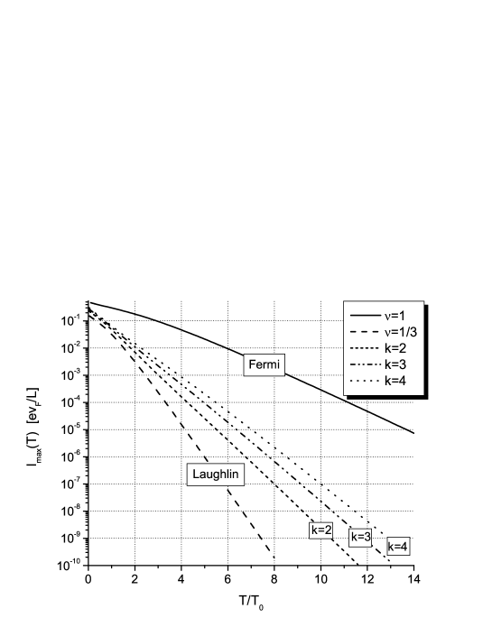
Figure 2: Logarithmic plot of the temperature decay of the persistent current’s amplitudes for the Fermi liquid ($\nu_{H}=1$), the Laughlin state ($\nu_{H}=1/3$) and the $k=2,3$ and $4$ parafermion FQH states

This universal thermal decoherence is described by the universal exponents $\alpha_{k}$, which determine the slopes of the logarithmic plots in Fig. 2. Notice that, unlike the Fermi/Luttinger liquids where $\alpha=\nu^{-1}$, $\alpha_{k}$ have a crucial neutral contribution

$$\alpha_{k}=\frac{1}{\nu_{H}}+2\Delta^{\mathrm{PF}_{k}}\left(\underline{\Lambda}_{0}+\underline{\Lambda}_{2}\right)=\frac{k+6}{k+2},$$ (7)

where $\Delta^{\mathrm{PF}_{k}}\left(\underline{\Lambda}_{0}+\underline{\Lambda}_{2}\right)=(k-2)/(k(k+2))$ is the neutral CFT dimension of the parafermion primary field with label $\underline{\Lambda}_{0}+\underline{\Lambda}_{2}$. Thus the universal decay exponents (7) can be considered the fingerprint of the FQH states.

References

• [1] S. D. Sarma, M. Freedman, and C. Nayak, “Topologically-protected qubits from a possible non-abelian fractional quantum Hall state,” Phys. Rev. Lett. 94 (2005) 166802, cond-mat/0412343.
• [2] A. Cappelli, L. Georgiev, and I. Todorov, “Parafermion Hall states from coset projections of abelian conformal theories,” Nucl. Phys. B 599 [FS] (2001) 499–530, hep-th/0009229.
• [3] L. Georgiev, “Chiral persistent currents and magnetic susceptibilities in the parafermion quantum Hall states in the second Landau level with Aharonov–Bohm flux,” Phys. Rev. B 69 (2004) 085305, cond-mat/0311339.
• [4] N. Read and E. Rezayi, “Beyond paired quantum Hall states: parafermions and incompressible states in the first excited Landau level,” Phys. Rev. B 59 (1999) 8084, cond-mat/9809384.
• [5] L. Georgiev and M. Geller, “Magnetic moment oscillations in a quantum Hall ring,” Phys. Rev. B 70 (2004) 155304, cond-mat/0404681.
• [6] J. Fröhlich and U. M. Studer, “Gauge invariance and current algebra in nonrelativistic many-body theory,” Rev. Mod. Phys. 65 (1993) 733.
• [7] J. Fröhlich, B. Pedrini, C. Schweigert, and J. Walcher, “Universality in quantum Hall systems: Coset construction of incompressible states,” J. Stat. Phys. 103 (2001) 527, cond-mat/0002330.
• [8] L. Georgiev, “A universal conformal field theory approach to the chiral persistent currents in the mesoscopic fractional quantum Hall states,” Nucl. Phys. B 707 (2005) 347, hep-th/0408052.
• [9] A. Cappelli and G. R. Zemba, “Modular invariant partition functions in the quantum Hall effect,” Nucl. Phys. B490 (1997) 595, hep-th/9605127.
• [10] U. Sivan and Y. Imry, “de Haas-van Alphen and Aharonov–Bohm-type persistent current oscillations in singly connected quantum dots,” Phys. Rev. Lett. 61 (1988) 1001.
• [11] M. Geller and D. Loss, “Aharonov–Bohm effect in the chiral Luttinger liquid,” Phys. Rev. B 56 (1997) 9692.
• [12] L. S. Georgiev and M. R. Geller, “Aharonov–Bohm effect in the non-abelian quantum Hall fluid,” (2005) cond-mat/0511236.
• [13] V. Kac and I. Todorov, “Affine orbifolds and rational conformal field theory extensions of ${W}_{1+\infty}$,” Commun. Math Phys. 190 (1997) 57–111, hep-th/9612078.
• [14] L. Georgiev, “The diagonal affine coset construction of the ${{\mathbb{Z}}}_{k}$ parafermion Hall states,” in Proc. of the Fifth Int. Workshop ”Lie Theory and its Applications in Physics”, June 2003, Varna, Bulgaria,, H.-D. Doebner and V. Dobrev, eds., pp. 301–310. World Scientific, 2003. hep-th/0402159.