MCTP-05-104

MIT-CTP-3740

NSF-KITP-05-117

UT-05-21

hep-th/0601054

Triangle Anomalies from Einstein Manifolds

Sergio Benvenuti¹, Leopoldo A. Pando Zayas^2,4
and Yuji Tachikawa^3,4

¹  Scuola Normale Superiore, Pisa,
and INFN, Sezione di Pisa, Italy.

²  Michigan Center for Theoretical Physics, Randall Laboratory of Physics,
The University of Michigan Ann Arbor, MI48109-1040,USA

³  Department of Physics, Faculty of Science,
University of Tokyo, Tokyo 113-0033, Japan

⁴ Kavli Institute for Theoretical Physics,
University of California, Santa Barbara, CA 93106, USA

Abstract

The triangle anomalies in conformal field theory, which can be used to determine the central charge $a$, correspond to the Chern-Simons couplings of gauge fields in ${\text{AdS}}_{5}$ under the gauge/gravity correspondence. We present a simple geometrical formula for the Chern-Simons couplings in the case of type IIB supergravity compactified on a five-dimensional Einstein manifold $X$. When $X$ is a circle bundle over del Pezzo surfaces or a toric Sasaki-Einstein manifold, we show that the gravity result is in perfect agreement with the corresponding quiver gauge theory. Our analysis reveals an interesting connection with the condensation of giant gravitons or dibaryon operators which effectively induces a rolling among Sasaki-Einstein vacua.

1 Introduction

Recent years have seen a tremendous progress in developing the Anti de Sitter/Conformal Field Theory (${\text{AdS}}_{5}/\text{CFT}_{4}$) correspondence [1]. The correspondence arises from considering a large number $N$ of D3-branes placed at a singularity, which is locally the tip of a real cone over a five-dimensional Einstein manifold $X$. It predicts the equivalence of the field theory on the stack of the D3-branes and the Type IIB theory on ${\text{AdS}}_{5}\times X$.

The very first check of the correspondence involves the symmetries on the two sides. The conformal group of $\text{CFT}_{4}$ is mapped to the isometry group of ${\text{AdS}}_{5}$. Other global symmetries in the $\text{CFT}_{4}$ are mapped to gauge symmetries in ${\text{AdS}}_{5}$. More precisely, global symmetry currents $J_{I}$ on the boundary correspond to massless gauge fields $A^{I}$ in the five-dimensional ($5$d) bulk with the boundary coupling $\int d^{4}x\,A^{I}J_{I}.$

The global symmetries in the CFT side in general have triangle anomalies among them. They are mapped to the Chern-Simons (CS) couplings $(24\pi^{2})^{-1}\int c_{IJK}A^{I}\wedge F^{J}\wedge F^{K}$ for the $5$d gauge fields, and the matching between them provides a quantitative check of the ${\text{AdS}}/\text{CFT}$ correspondence. It was carried out in [2] for $X=S^{5}$ using supergravity results of [3, 4], but it has not yet been done for other Einstein manifolds. It is well-known that triangle anomalies can be extracted by a simple one-loop computation in the gauge theories, and that they are topological objects. We thus expect that it should be possible to develop a generic quantitative understanding also on the gravity side of the duality, because they should belong to “protected sectors” of the ${\text{AdS}}_{5}/\text{CFT}_{4}$ correspondence.

Other types of “protected sectors” of the ${\text{AdS}}/\text{CFT}$ correspondence are given by the Bogomol’ny-Prasad-Sommerfield (BPS) operators, which are protected by supersymmetry. In this case one can map the scaling dimensions of the BPS operators to the energy of the corresponding BPS states in type IIB string theory on ${\text{AdS}}_{5}\times X$. We can expect it to be possible to understand the dual BPS objects on the gravity side in general, without the need of having the explicit metrics. This is indeed the case, for instance, for dimensions of baryonic BPS operators, corresponding to the volumes of supersymmetric (SUSY) cycles, which can be computed with the procedure uncovered in [5]. In the same way, we expect that the CS coefficients can be calculated in the gravity side without the knowledge of the explicit metrics.

The $5$d Chern-Simons coefficients also appear prominently in the analysis of M-theory on Calabi-Yau threefolds. They are given in terms of the triple intersections of three four-cycles of the Calabi-Yau. Hence, we expect to find a similarly robust formula for the CS coefficients in the case of Type IIB supergravity on compact, positively curved, Einstein manifolds $X$.

Thus, our first objective is to obtain a geometrical formula for the Chern-Simons coefficients $c_{IJK}$ for Type IIB supergravity on ${\text{AdS}}_{5}\times X$. The result we will obtain is so elegant that we would like to give the formula here. It is given by

$$c_{IJK}=\frac{N^{2}}{2}\int_{X}\omega_{\{I}\wedge\iota_{k_{J}}\omega_{K\}}\,.$$ (1.1)

Here, $N$ is the number of the flux of the self-dual five-form $F_{5}$ through $X$, and three-forms $\omega_{I}$ of $X$ appears in the fluctuation of $F_{5}$ via

$$\delta F_{5}=N(A^{I}\wedge\omega_{I})$$ (1.2)

where $A^{I}$ are gauge fields on ${\text{AdS}}_{5}$. Therefore $\omega_{I}$ determines the the distribution of $F^{I}$ in the internal manifold and thus is usually called wave function.

The Killing vectors $k_{I}$ measure the non-closedness of $\omega_{I}$ by the relation

$$d\omega_{I}+\iota_{k_{I}}\mathrm{vol}^{\circ}=0$$ (1.3)

where $\mathrm{vol}^{\circ}$ is the volume form normalized to have $\int_{X}\mathrm{vol}^{\circ}=1$. The index $I$ runs from $1$ to $d=\ell+b^{3}$ where $\ell$ is the number of isometries of $X$ and $b^{3}$ is the third Betti number of $X^{5}$.

We will show that this formula gives robust topological quantities in a precise sense. In particular, explicit knowledge of the Einstein metric on $X$ is not necessary to evaluate the formula (1.1).

While our formula (1.1) is valid for any Einstein manifold $X$, the case when $X$ is Sasaki-Einstein (SE) is especially interesting. In this case, by definition, the cone over $X$ is Calabi-Yau. Then, minimal $\mathcal{N}=1$ supersymmetry is preserved and we get an $\mathcal{N}=1$ superconformal field theory (SCFT). Other than the round $S^{5}$, the only Sasaki-Einstein space with an explicitly known metric was $T^{1,1}$ for a long time; its SCFT dual was first studied by Klebanov and Witten in [6]. We now have a countably infinite number of explicit SE metrics [7, 8, 9] and the corresponding quiver gauge theories [10, 11, 12, 13]. There is a nice interaction between ‘topological’ objects and objects protected by supersymmetry. Thus, we have many examples to test our formula against field theory expectations.

For generic $4$d $\mathcal{N}=1$ SCFTs, triangle anomalies encode a lot of physical information and are related to various important correlators of the symmetry currents and the energy-momentum tensor [14]. In particular, the supersymmetric partner of the energy-momentum tensor is an Abelian global symmetry, which is called the $R$-symmetry. One important point in ${\text{AdS}}/\text{CFT}$ correspondence is that the triangle anomaly of the $R$-symmetry, $c_{RRR}$, which is the central charge $a$ of the SCFT [14], is inversely proportional to the volume of the SE manifold [15, 16].

Quantitative analysis on the field theory side can be done thanks to ‘$a$-maximization’ [17], which determines the $R$-symmetry. On the gravity side the $R$-symmetry is mapped to the so-called ‘Reeb vector’ of the internal manifold $X$. In the case $X$ is toric Sasaki-Einstein, i.e. the isometry group of $X$ contains a $U(1)^{3}$, ‘$Z$-minimization’ [5] determines the Reeb vector; it is thus possible to compare the volume of $X$ and of SUSY $3$-cycles with gauge theory, as was done in [18]. In the case of the recently found $Y^{p,q}$ and $L^{p,q,r}$, checks of the duality have been given for $c_{RRR}$ in [10, 19], for BPS mesonic operators in [20, 11, 21, 22] and for various SUSY branes in [23]. There are also works which clarify the relation between $a$-maximization and $Z$-minimization through 5d theory in ${\text{AdS}}_{5}$ [24, 25]. Note that their results are valid also in the non-toric case.

We enlarge this impressive list of checks of the correspondence by providing an explicit evaluation of $c_{IJK}$, through (1.1), for large sets of Sasaki-Einstein manifolds, namely, circle bundles over del Pezzo surfaces and toric Sasaki-Einstein manifolds. The evaluation utilizes the flow triggered by the condensation of the giant gravitons. We analyze the field theory side using the same flow by the Higgsing using the dibaryon operators, and we find complete agreement on the gravity side and the field theory side. For toric SE we obtain

$$c_{IJK}=\frac{N^{2}}{2}|\det(k_{I},k_{J},k_{K})|$$ (1.4)

where $k_{I}\in\mathbb{Z}^{3}$ is the $I$-th generator of the toric cone. We also call $k_{I}$ the toric data, as is customary in string theory literature. In other words, $c_{IJK}$ is simply given by the area of a triangle formed by the three toric data. We recover the formula (1.4) from field theory, thus providing a very general check of ${\text{AdS}}/\text{CFT}$.

We will also analyze the BPS operators which are related to giant gravitons, emphasizing the interplay between objects protected by SUSY and topological properties of $X$. Throughout the analysis, we will see that there is an intricate mixing of the angular momenta and baryonic charges, which reflects the fact that the D3-branes wrapping three-cycles in the SE manifold is partly a giant graviton. This unifies the study of two kind of supersymmetric states important for the AdS/CFT correspondence. One is the giant gravitons, corresponding to determinant operators in $\mathcal{N}=4$ super Yang-Mills, and the other is the D3-branes wrapped on supersymmetric $3$-cycles, corresponding to dibaryon operators in the dual quiver theory.

The organization of this paper is the following: first we sketch in section 2 the supergravity reduction which gives the formula for the CS terms and gauge coupling constants. Then, we discuss the normalization of gauge fields and the charges in section 3, where we will see that the formula for the CS terms is topological in a precise sense. We evaluate the formulae for toric Sasaki-Einstein manifolds and for the circle bundles over del Pezzo surfaces in section 4. In section 5, we turn to field theory dual and show, based on explicit examples, that the results obtained in previous sections match with predictions based on ${\text{AdS}}_{5}/\text{CFT}_{4}$ correspondence. In section 6, we explain the simplicity of our results in section 5 using the flow triggered by the condensation of dibaryons. We conclude with some discussions in section 7. Appendix A contains the detail of the supergravity reduction, while in appendix B we obtain the triangle anomaly for quiver theories corresponding to generic toric Sasaki-Einstein manifolds. Finally in appendix C, we elaborate on the mathematics behind the charge lattice associated to the five-dimensional Einstein manifold with isometries.

2 Perturbative Supergravity Reduction

Consider Type IIB theory on ${\text{AdS}}_{5}\times X$ where $X$ is an Einstein manifold of dimension five. Let us carry out the Kaluza-Klein reduction and retain only the massless gauge fields. The corresponding five-dimensional action has the form

$$S=\frac{1}{2}\int\tau_{IJ}F^{I}\wedge*F^{J}+\frac{1}{24\pi^{2}}\int c_{IJK}A^{I}\wedge F^{J}\wedge F^{K}+\cdots,$$ (2.1)

which yields the equation of motion

$$\tau_{IJ}d*F^{I}=\frac{1}{8\pi^{2}}c_{IJK}F^{J}\wedge F^{K}.$$ (2.2)

We would like to calculate the Chern-Simons interaction $c_{IJK}$ of the gauge fields. We will eventually choose the indices $I,J,\ldots$ to label the integral basis of the gauge fields in the next section, but in this section we take them arbitrarily. We chose the numerical coefficient $(24\pi^{2})^{-1}$ so that $c_{IJK}=\operatorname{tr}Q_{I}Q_{J}Q_{K}$ under the AdS/CFT correspondence, where $Q_{I}$ is the global symmetry corresponding to the gauge field $A_{I}$, and the trace is over the label of Weyl fermions.

The arguments which are to be presented in sections 2.1 and 2.2 only uses the fact that the metric is Einstein, so it is applicable, e.g. to the manifolds $T^{a,b}$ for $(a,b)\neq(1,1)$.

2.1 The Ansatz and its reduction

Since the detail of the reduction is rather tedious, we present only a rough argument in this section. Interested readers can consult appendix A for the details. We use three kinds of Hodge stars, namely on $X$, on ${\text{AdS}}_{5}$ and on ${\text{AdS}}_{5}\times X$. We denote the last one by $*_{10}$, and the first two by $*$. We hope the context makes clear which one we used.

The equations of motion and the Bianchi identity in Type IIB supergravity are

$$R_{\mu\nu}=\frac{c}{24}F_{\mu\alpha\beta\rho\sigma}F_{\nu}{}^{\alpha\beta\rho\sigma},\qquad F_{5}=*_{10}F_{5},\qquad dF_{5}=0$$ (2.3)

where $R_{\mu\nu}$ is the Ricci curvature of the ten-dimensional metric and $F_{5}$ is the self-dual five-form field strength. The constant $c$ depends on conventions. We set all other form fields and fermions to zero, and the dilaton to constant throughout the analysis.

Let $N$ units of five-form flux penetrate $X$, where we normalize the five-form $F_{5}$ to have $\int F_{5}\in 2\pi\mathbb{Z}$. The zero-th order solution is

$$ds^{2} =L^{2}ds^{2}_{{\text{AdS}}}+L^{2}ds^{2}_{X},$$ (2.4)

$$F_{5} =\frac{2\pi N}{V}\left(\mathrm{vol}_{X}+\mathrm{vol}_{{\text{AdS}}}\right).$$ (2.5)

where $\mathrm{vol}$ is the volume form of $X$ and $V=\int_{X}\mathrm{vol}$. We take the convention $R_{\mu\nu}=-4g_{\mu\nu}$ for $ds^{2}_{{\text{AdS}}}$ and $R_{\mu\nu}=4g_{\mu\nu}$ for $ds^{2}_{X}$as usual. $L$ sets the physical length scale.

Suppose $X$ has $\ell$ $U(1)$ isometries $k_{a}^{i}$, ($a=1,\ldots,\ell$) so that $\exp(2\pi k_{a}^{i}\partial_{i})$ is the identity. For toric SE manifolds, $\ell=3$. Let us expand the fluctuation around the zero-th order solution in modes. One can consistently set to zero all the modes which are not invariant under the $U(1)$ isometries. We take the usual Kaluza-Klein ansatz for the metric

$$ds^{2}_{X}=\sum_{i}(e^{i}+k_{a}^{i}A^{a})^{2}$$ (2.6)

where $e^{i}$ are the fünfbein forms of the compact manifold $X$, and $A^{a}$ are one-forms on ${\text{AdS}}_{5}$.

The Ansatz for $F_{5}$ is rather intricate already at first order. We write $F_{5}$ as the sum of components $F_{p,q}$ which has $p$ legs in ${\text{AdS}}_{5}$ and $q$ legs in $X$ so that

$$F_{5}=F_{0,5}+F_{1,4}+F_{2,3}+F_{3,2}+F_{4,1}+F_{5,0}.$$ (2.7)

Then we take the Ansatz to be

$$F_{0,5} =\frac{2\pi N}{V}\mathrm{vol}_{X}, F_{5,0} =\frac{2\pi N}{V}\mathrm{vol}_{{\text{AdS}}},$$ (2.8)

$$F_{1,4} =\frac{2\pi N}{V}A^{a}\wedge\iota_{k_{a}}\mathrm{vol}_{X}+*F_{4,1},$$ (2.9)

$$F_{2,3} =NF^{I}\wedge\omega_{I}, F_{3,2} =N(*F^{I})\wedge*\omega_{I}.$$ (2.10)

Here, $\omega_{I}$ are three-forms on $X$ to be determined later, and $F^{I}$ are two-forms on ${\text{AdS}}_{5}$, respectively. The range in which $I$ can take values is also determined later. The first term in (2.9) is necessary because eq. (2.6) modifies the Hodge star.

The exterior derivative is decomposed to $d=d_{X}+d_{\text{AdS}}$ where $d_{X,{\text{AdS}}}$ is the exterior derivative on the respective spaces. Then, $dF_{5}=0$ imposes

$$d_{\text{AdS}}F_{p,q+1}+d_{X}F_{p+1,q}=0.$$ (2.11)

$F_{4,1}$ can be shown to yield massive degrees of freedom, so we set $F_{4,1}=0$. Moreover, in order to have massless equation of motion $dF^{I}=0$ and $d*F^{I}=0$, there must be constants $c^{a}_{I}$ such that

$$d*\omega_{I}=0,\qquad d\omega_{I}=\frac{2\pi}{V}c^{a}_{I}\iota_{k_{a}}\mathrm{vol}_{X},$$ (2.12)

for $\omega_{I}$ and

$$dA^{a}=c^{a}_{I}F^{I}$$ (2.13)

for $F^{I}$. One important property is the non-closedness of $\omega_{I}$, which was already pointed out in [25]. If $d\omega_{I}=0$ in (2.12), the allowed number of $F^{I}$ would be precisely $b^{3}=\dim H^{3}(X)$. The presence of $\iota_{k_{a}}\mathrm{vol}_{X}$ enlarges the dimension of the space of wavefunctions $\omega_{I}$ for massless gauge fields by the number of isometries, $\ell$. Thus, the index $I$ runs from $1$ to $d$ where

$$d=\ell+b^{3}.$$ (2.14)

Let us introduce $\mathrm{vol}^{\circ}\equiv\mathrm{vol}/V$ and $k_{I}\equiv 2\pi c^{a}_{I}k_{a}$. Eq. (2.12) becomes

$$d\omega_{I}+\iota_{k_{I}}\mathrm{vol}_{X}^{\circ}=0.$$ (2.15)

We now consider the Chern-Simons couplings. One contribution to the CS interaction arises as follows. The Hodge star $*$ for the metric ansatz (2.6) forces $F_{5}$ to have a second-order contribution of the form

$$\delta^{(2)}F\propto A^{a}\wedge F^{I}\wedge\iota_{k_{a}}\omega_{I},$$ (2.16)

just as we had $A^{a}\wedge\iota_{k_{a}}\mathrm{vol}_{X}$ term in (2.9). Then, $d_{\text{AdS}}F_{3,2}+d_{X}F_{4,1}=0$ requires the presence of $F^{a}\wedge F^{I}$ terms in the right hand side of the equation of motion. After combining with the other contribution, the resulting equation of motion for $F^{I}$ turns out to be

$$d*F^{I}\int_{X}(\omega_{K}\wedge*\omega_{I}+\frac{1}{16V^{2}}(k_{K}\cdot k_{I})\mathrm{vol})=\frac{1}{8\pi}F^{I}\wedge F^{J}\int_{X}\omega_{\{I}\wedge\iota_{k_{J}}\omega_{K\}}$$ (2.17)

where $(a\cdot b)$ for two one-forms $a=a_{i}dx^{i}$, $b=b_{i}dx^{i}$ is defined by $(a\cdot b)=a_{i}b_{j}g^{ij}$, and $\{IJK\}=IJK+IKJ+\cdots$ is the total symmetrization without $1/6$. Again, consult appendix A for details.

2.2 Comparison to the 5d Lagrangian

Let us write down the formula for $c_{IJK}$ and $\tau_{IJ}$. In order to determine the combination of $\tau_{IJ}$ and $c_{IJK}$ entering the five-dimensional action, we need the normalization of the kinetic term of $F_{5}$ entering the ten-dimensional action. One can resort to string worldsheet perturbation theory, but there is a quicker way out. We are normalizing $F_{5}$ to have $\int F_{5}\in 2\pi\mathbb{Z}$. Then a D3-brane sources the field $F_{5}=dC_{4}$ by the coupling $S=\int_{D3}C_{4}$. D3-branes are their own electromagnetic dual, thus one D3-brane should create five-form flux which satisfies the same quantization condition $\int F_{5}\in 2\pi\mathbb{Z}$. Thus the supergravity action for $F_{5}$ is fixed to be

$$S_{F_{5}}=\frac{1}{4\pi}\int_{{\text{AdS}}\times X}\mathcal{F}_{5}\wedge*\mathcal{F}_{5}$$ (2.18)

where $\mathcal{F}_{5}=F_{0,5}+F_{1,4}+F_{2,3}$.

Plugging (2.6) and (2.10) into the ten-dimensional action, we obtain

$$\tau_{IJ}=\frac{N^{2}}{2\pi}\int_{X}(\omega_{J}\wedge*\omega_{I}+\frac{1}{16V^{2}}(k_{J}\cdot k_{I})\mathrm{vol})$$ (2.19)

where the first and second terms come from the kinetic terms for the five-form and the metric, respectively. This expression for $\tau_{IJ}$ agrees with the one presented in [25]. Then, from (2.17), we finally obtain

$$c_{IJK}=\frac{N^{2}}{2}\int_{X}\omega_{\{I}\wedge\iota_{k_{J}}\omega_{K\}}.$$ (2.20)

2.3 $a$ and the volume

Before moving to the explicit evaluation of $c_{IJK}$ for various Sasaki-Einstein manifolds, let us determine the central charge $a$ from our formula (2.20), and check that it is inversely proportional to the volume. In this subsection, we assume $X$ is not just an Einstein manifold but also is Sasaki-Einstein.

Let $J$ be the Kähler form of the cone $C(X)$ over $X$, and $e_{r}=r\partial_{r}$ the dilation on the cone direction. Let $e$ be the one-form $\iota_{e_{r}}J$. It endows $X$ with the structure of a contact manifold so that $\mathrm{vol}_{X}=e\wedge J\wedge J/2$ and $de=2J$. The Reeb vector is $ie_{r}$.

Since $X$ is now Sasaki-Einstein, the corresponding CFT is $\mathcal{N}=1$ supersymmetric. Let the R-symmetry in the superconformal algebra be the linear combination $R^{I}Q_{I}$. Then, the central charge $a$ is given by

$$a=\frac{9}{32}c_{IJK}R^{I}R^{K}R^{K}=\frac{N^{2}}{2}\frac{27}{16}\int\omega_{R}\wedge\iota_{k_{R}}\omega_{R}$$ (2.21)

where $\omega_{R}=R^{I}\omega_{I}$ and $k_{R}=R^{I}k_{I}$. It is known through the work [26] that $\omega_{R}$ is a multiple of $e\wedge J$. We should normalize it so that $k_{R}$ is proportional to the Reeb vector, and the holomorphic three-form $\Omega$ on $C(X)$ has charge $2$ under $k_{R}$. Thus, we obtain

$$k_{R}=2\pi\frac{2}{3}ie_{r}$$ (2.22)

because $\Omega$ scales as $r^{3}$ and the natural holomorphic one-form is $re$. The extra factor of $2\pi$ comes from our convention $k_{I}=2\pi c^{a}_{I}k_{a}$ relating $k_{I}$ and the $k_{a}$ in the metric ansatz.

Thus, we have

$$\omega_{R}=-\frac{\pi e\wedge J}{3V}$$ (2.23)

from (2.15). Then eq (2.21) becomes

$$a=\frac{N^{2}}{2}\frac{27}{16}\frac{4\pi^{3}}{27}\frac{\int e\wedge J\wedge J}{V^{2}}=\frac{N^{2}}{4}\frac{\pi^{3}}{V},$$ (2.24)

which is precisely the relation established in [15, 16].

3 Properties of the supergravity formula

3.1 Giant Gravitons and the normalization of $\omega_{I}$

We have found so far the formula (2.20) for the CS coefficient $c_{IJK}$ given in terms of three-forms $\omega_{I}$ on the Einstein manifold $X$. The gauge field in the AdS space has these forms as wavefunctions. In order to compare the result to the field theory in four dimensions, first we need to find the basis of the gauge fields so that charged objects have integral charges with respect to these gauge fields.

Let us recall the situation in the compactification of the M-theory on a Calabi-Yau $Y$. In that case, a massless gauge field arises from the M-theory three-form with a harmonic two-form $\omega$ on $Y$ as the wavefunction, and harmonic two-form naturally corresponds to $H^{2}(Y,\mathbb{R})$. M2-branes wrapped on a two-cycle $C$ in the Calabi-Yau give rise to the charged particles in the noncompact dimensions, and the charge is given by $\int_{C}\omega$. Thus, $H^{2}(Y,\mathbb{Z})\subset H^{2}(Y,\mathbb{R})$ gives the integral basis we wanted.

Similarly in our case, D3-branes wrapped on three-cycles in the Einstein manifold $X$ give rise to charged objects in the AdS side. There are $b^{3}(X)$ homologically independent three-cycles. We also have $\ell$ Kaluza-Klein angular momenta associated to the $\ell$ isometries. For example, gravitons moving inside $X$ will give charged objects from the AdS point of view. In all, there are $d=b^{3}(X)+\ell$ types of charged objects which match the number of the massless gauge fields.

Let us give a simple argument showing that ordinary homology of 3-cycles is not the correct mathematical object to classify the charges of the supersymmetric wrapped D3-branes. For $S^{5}$ the homology is trivial but there are giant gravitons. A less simple example comes from the $Y^{p,q}$ geometries (where the topology is simply $S^{2}\times S^{3}$): there are various supersymmetric 3-cycles which are homologically equivalent but have different volumes. D3-branes wrapped on different cycles correspond to different operators in the dual quiver gauge theory. These SUSY 3-cycles are invariant under the $U(1)^{l}=U(1)^{3}$ isometries. The point is that we cannot deform one such SUSY 3-cycle to another keeping it invariant under the isometries. It is thus clear that we need some kind of homology that keeps track also of the isometries, which show up in ${\text{AdS}}_{5}$ as Kaluza-Klein momenta.

Alert readers might be puzzled by now by the fact that the wavefunctions $\omega_{I}$ are not closed in general. Then the charge of a wrapped D3-brane depends not only on its homology class, but also on extra data, as expected also from the discussion in the previous paragraph. The Kaluza-Klein gauge fields coming from the metric also enter the expansion of $F_{5}$, because in the expansion (2.10)

$$\delta F_{5}=d(A^{I}\wedge N\omega_{I}),$$ (3.1)

$A_{I}$ includes the gauge fields from the metric through (2.13). The non-closedness of $\omega_{I}$ allows a D3-brane wrapping a topologically trivial cycle $C$ to have non-zero coupling to $A^{I}$ given by

$$N\int_{C}\omega_{I}.$$ (3.2)

For instance, if we consider Type IIB theory on $S^{5}$ with $N$ units of five-form flux and we wrap a D3-brane on $S^{3}$ at the equator, it will give rise to a soliton with $N$ unit of Kaluza-Klein momenta. This is precisely the maximal giant gravitons treated in [28, 29].

For simplicity, let us restrict our attention to branes which are not moving in the SE. In order for them to be charge eigenstates, their worldvolume should be invariant under the isometry. Let us introduce an equivalence relation such that $C\sim C^{\prime}$ if $C-C^{\prime}=\partial B$ where $B$ is an invariant four-chain. Then, the coupling of the branes to the gauge fields $A^{I}$ depends only on the equivalence class, because

$$\int_{C}\omega_{I}-\int_{C^{\prime}}\omega_{I}=\int_{\partial B}\omega_{I}=\int_{B}d\omega_{I}=\int_{B}\iota_{k_{I}}\mathrm{vol}^{\circ},$$ (3.3)

and the integral of $\iota_{k}$ acting on anything vanishes if the integration region $B$ is invariant under $k$. It is because the integrand is zero when $k$ is degenerating on $B$ and the interior product kills the legs along $B$ when $k$ does not degenerate on $B$.

Suppose $X$ has $U(1)^{\ell}$ isometry and the third Betti number is $b^{3}$. In the explicit examples we will treat in the following sections, there are always $d=\ell+b^{3}$ of independent invariant three-cycles, although we could not find a general proof in the mathematical literature. Assuming this, D3-branes wrapping on invariant three-cycles comprise a good basis of charged objects with respect to the gauge fields $A^{I}$. Let us denote the basis by $C^{I}$, ($I=1,\ldots,d$). Then,

$$\int_{C^{I}}\omega_{J}=\delta^{I}_{J},$$ (3.4)

determines the dual basis for the wavefunctions of the gauge fields $A_{I}$. Then a D3-brane wrapping the cycle $C^{I}$ has charge $N$ under $A_{I}$, and charge $0$ for other gauge fields.

3.2 Metric independence of $c_{IJK}$

First we recall the situation for the M-theory on Calabi-Yau 3-fold case. There, after the Kaluza-Klein reduction, the five-dimensional Chern-Simons interaction $c_{IJK}$ of the massless gauge fields $A^{I}$ is given by

$$c_{IJK}\propto\int\omega_{I}\wedge\omega_{J}\wedge\omega_{K}$$ (3.5)

where $\omega_{I}$ is the two-form on the Calabi-Yau which appears in the Kaluza-Klein Ansatz for the M-theory three-form $C$,

$$\delta C=A^{I}\wedge\omega_{I}.$$ (3.6)

The masslessness of $A_{I}$ requires $\omega_{I}$ to be harmonic, and explicitly finding the harmonic form is quite difficult. Fortunately, the formula above (3.5) is independent of the shift of $\omega_{I}$ by exact forms. It implies that $c_{IJK}$ becomes independent of the metric.

Similarly, we found in sec. 2 the form $\omega_{I}$ is co-closed and ‘closed up to isometry’ (2.15). We show in this section that $c_{IJK}$ and the normalization condition do not change under the shift

$$\omega_{I}\to\omega_{I}+d\alpha_{I}+\iota_{k_{I}}\beta$$ (3.7)

where $\alpha_{I}$ are two-forms, $\beta$ is a four-form, both of which are assumed to be invariant under $U(1)^{\ell}$ action.

First we discuss the shift $\omega_{I}\to\omega_{I}+d\alpha_{I}$. The normalization condition (3.4) is not affected. The change in $c_{IJK}$ is zero because

$$\delta c_{IJK}\propto\int d\alpha_{\{I}\wedge\iota_{k_{J}}\omega_{K\}}=-\int\alpha_{\{I}\wedge\iota_{k_{J}}d\omega_{K\}}\\ =-\int\alpha_{\{I}\wedge\iota_{k_{J}}\iota_{k_{K\}}}\mathrm{vol}_{X}^{\circ}=0.$$ (3.8)

Secondly, we turn to the shift $\omega_{I}\to\iota_{k_{I}}\beta$. Here, we need to shift all of the forms $\omega_{I}$ simultaneously using the same $\beta$. It induces the change in $c_{IJK}$ by

$$\delta c_{IJK}=\int\iota_{k_{\{I}}\beta\wedge\iota_{k_{J}}\omega_{K\}} =0.$$ (3.9)

Hence it does not change the CS coefficient. As for the normalization (3.4), the cycles $C^{I}$ are assumed to be invariant under the isometry. Then we have $\int_{C^{I}}\iota_{k_{J}}\beta=0$, using the same argument as before.

From the relation (2.15), the shift $\omega_{I}\to\iota_{k_{I}}\beta$ is accompanied by the shift $\mathrm{vol}^{\circ}\to\mathrm{vol}^{\circ}-d\beta$. It means that we are free to take any five-form which integrates to one as $\mathrm{vol}^{\circ}$ in determining $\omega_{I}$ through (2.15). The equation (2.15) fixes $\omega_{I}$ only up to the addition of exact forms, which was shown not to affect $c_{IJK}$ above.

Let us recapitulate the method to calculate $c_{IJK}$.

• We first take any invariant five-form $\mathrm{vol}^{\circ}$ which satisfies $\int\mathrm{vol}^{\circ}=1$.

• Then find $\omega_{I}$ with the normalization $\int_{C^{J}}\omega_{I}=\delta^{J}_{I}$, (3.4).

• Next we define $k_{I}$ as the linear combination of $\ell$ isometries such that the condition $d\omega_{I}+\iota_{k_{I}}\mathrm{vol}^{\circ}=0$, (2.15) is satisfied.

• Finally we plug these quantities to the formula (2.20) and evaluate.

The procedure does not require knowledge of the Einstein metric on $X$. We would like to emphasize that the Sasaki structure on $X$ is not necessary in the calculation of $c_{IJK}$ either. The only ingredient is the action of $U(1)^{\ell}$ on $X$. In this sense we claim that $c_{IJK}$ is a topological invariant of the manifold with $U(1)^{\ell}$ action.

4 Explicit Evaluation of the supergravity formula

4.1 Sasaki-Einstein manifolds with one $U(1)$ isometry

We first treat the case where there is only one isometry $k$ on the Sasaki-Einstein manifold $X$. We take the period of $k$ to be $2\pi$. Then, the isometry determines on $X$ an $S^{1}$ fibration

$$\begin{array}[]{ccc}S^{1}&\to&X\\ &&\downarrow\\ &&B\end{array}$$ (4.1)

over a Kähler-Einstein base $B$. Let the one-form $e$ be $e=g_{ij}k^{i}dx^{j}$. Then, the Sasaki-Einstein condition implies that the curvature of the circle bundle $de$ is equal to twice the Kähler class $J$ of the base $B$, that is,

$$de=2J.$$ (4.2)

We have $\mathrm{vol}^{\circ}\propto e\wedge J\wedge J$. Then, an elementary calculation shows that elements of $H^{3}(X)$ corresponds to elements of $H^{2}(B)$ annihilated by $J\wedge$. Thus, $b^{3}(X)=b^{2}(X)-1$. Since we assumed $\ell=1$, the number of the gauge field $d$ is

$$d=\ell+b^{3}(X)=b^{2}(B).$$ (4.3)

Thus, we need to find $b^{2}(B)$ of three-cycles $C^{I}$ and three-forms $\omega_{I}$ in $X$ which satisfy the constraint (2.15) and (3.4). To this end, take a basis of two-cycles $D^{1},\ldots,D^{d}$ in $B$ and the dual basis of two-forms $\gamma_{1},\ldots,\gamma_{d}$ on $B$ such that $\int_{D^{I}}\gamma_{J}=\delta^{I}_{J}$. Let us take $C^{I}$ to be the three-cycle above $D^{I}$ in the fibration and $\omega_{I}=(2\pi)^{-1}e\wedge\gamma_{I}$. Then the normalization (3.4) is automatic, and from $d\omega_{I}+\iota_{k_{I}}\mathrm{vol}^{\circ}=0$ (2.15), we have

$$k_{I}=-2(\int_{B}J\wedge\gamma_{I})k.$$ (4.4)

Thus we obtain

$$c_{IJK}=\frac{N^{2}}{2}\int_{B}\frac{J}{\pi}\wedge\gamma_{\{I}\int_{B}\gamma_{J}\wedge\gamma_{K\}}.$$ (4.5)

4.2 Higher del Pezzo surfaces

Circle bundles over del Pezzo surfaces are prime examples of five-dimensional Sasaki-Einstein manifolds, where the $n$-th del Pezzo surface $dP_{n}$ for $n<9$ is $\mathbb{CP}^{2}$ blown up at generic $n$ points. For $n=1,2,3$ they are toric, which will be treated in the next subsection. In this subsection we evaluate (4.5) for del Pezzo surfaces with $n\geq 4$, which have only one isometry which rotates the circle fiber. We compare the result with the field theory result in section 5.2.

Let us take $\gamma_{0}$ as the two-form dual to the base $\mathbb{CP}^{2}$, and $\gamma_{i}$, $i=1,\ldots,n$ be the two-forms dual to the $i$-th exceptional cycle. The intersection paring is Lorentzian, i.e.

$$\int_{dP_{n}}\gamma_{I}\wedge\gamma_{J}=\operatorname{diag}(+1,-1,\ldots,-1).$$ (4.6)

where $I,J=0,1,\ldots,n$. The Kähler form $J$ is chosen to be equal to negative of the Chern class of the anti-canonical bundle,

$$J=\frac{\pi}{3}(3\gamma_{0}-\sum_{i=1}^{n}\gamma_{i}).$$ (4.7)

The area of the $dP_{n}$ is $\int_{dP_{n}}J\wedge J/2=\pi^{2}(9-n)/18$. Formula (4.5) can be conveniently packed in the cubic polynomial

$$P_{n}(a_{0},a_{1},\ldots,a_{n})\equiv c_{IJK}a^{I}a^{J}a^{K}=3N^{2}\int_{dP_{n}}\frac{J}{\pi}\wedge\gamma\int_{dP_{n}}\gamma\wedge\gamma$$ (4.8)

by introducing indeterminate variables $a^{I}$, $I=0,\ldots,n$ and $\gamma\equiv\gamma_{I}a^{I}$. It can be easily evaluated to be

$$P_{n}(a^{I})=N^{2}\left(3a^{0}+\sum_{i}a^{i}\right)\left((a^{0})^{2}-\sum_{i}(a^{i})^{2}\right).$$ (4.9)

An obvious consequence is that we have

$$P_{n}(a^{0},a^{1},\ldots,a^{n})=P_{n+1}(a^{0},a^{1},\cdots,a^{n},a^{n+1}=0).$$ (4.10)

We will see the physical mechanism behind this result in later sections.

4.3 Toric Sasaki-Einstein manifolds

We would like to move on to the case where there are three isometries in the Sasaki-Einstein manifold $X$, i.e. $\ell=3$. In that case, the Calabi-Yau cone over $X$ is toric, thus $X$ is called a toric Sasaki-Einstein manifold. Let us describe $X$ as a $T^{3}$ fibration over a two-dimensional $d$-gon $B$, where the coordinates of $T^{3}$ are $\theta_{1,2,3}$ and those of the base are $y^{1,2}$. We take the periodicity of $\theta_{i}$ to be $1$. Denote the edges by $E^{I}$, $I=1,\ldots,d$, the 3-cycles above them by $C^{I}$. It is known that $H^{3}(X)=d-3$ so that the number of the edges is precisely the number of gauge fields which we obtain by compactifying Type IIB string on $X$. Let $k_{I}=k_{iI}\partial/\partial\theta_{i}$ be the degenerating Killing vector at $C^{I}$, see figure 1.

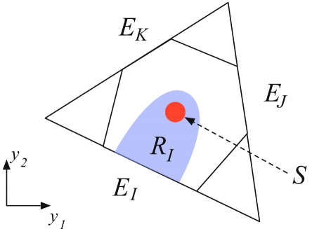
Figure 1: Construction of $\omega_{I}$. The polygon designates the image of the moment map. The red blob $S$ is the support of $\mathcal{F}$ and the blue region $R_{I}$ is the support of $\mathcal{A}_{I}$.

We will see shortly that the calculation of $c_{IJK}$ only depends on $k_{I,J,K}$ and not on the other $k_{L\neq I,J,K}$ or the number of the edges. From now on, all the forms are assumed to depend only on $y^{1,2}$.

Firstly, take a two-form $\mathcal{F}$ on the base $B$ supported on a region $S$ with $\int\mathcal{F}=1$. $S$ is marked with red in the figure 1. Choose

$$\mathrm{vol}^{\circ}=\mathcal{F}\wedge d\theta_{1}\wedge d\theta_{2}\wedge d\theta_{3}$$ (4.11)

as the normalized volume form.

Secondly, for each edge $E_{I}$, draw a region $R_{I}$ which contains $S$ and touches only with $E_{J}$ with $J=I$ (cf. fig. 1). Choose the one-form $\mathcal{A}_{I}$ on the base $B$ which is non-zero only in $R_{I}$ such that $d\mathcal{A}_{I}=\mathcal{F}$. Notice that $\int_{E^{I}}\mathcal{A}_{J}=\delta^{I}_{J}$, since $\mathcal{A}_{J}$ is only nonzero on $R_{J}$ and $\sum_{J}\int_{E_{J}}\mathcal{A}_{I}=\int_{B}\mathcal{F}=1$.

We need to ensure furthermore that $\mathcal{A}_{I}$ has only components parallel to the edge $E_{I}$. Then

$$\omega_{I}\equiv-\mathcal{A}_{I}\wedge\iota_{k_{I}}d\theta_{1}\wedge d\theta_{2}\wedge d\theta_{3}\qquad(\text{no summation on $I$})$$ (4.12)

is a well-behaved form on $X$, since the existence of $\iota_{k_{I}}$ guarantees that $\omega_{I}$ is regular near $E_{I}$, and the fact $A_{I}$ vanishes outside the blue region guarantees $\omega_{I}$ is regular near $E_{J\neq I}$. It also satisfies the constraint (2.15) and (3.4) almost by construction.

Now we can clearly see that the forms $\omega_{I,J,K}$ can be taken to be the same irrespectively of, for example, whether we are calculating $c_{IJK}$ for the hexagon inside or the triangle outside in the figure. Thus, $c_{IJK}$ depends only on $k_{I,J,K}$ and not at all on $k_{L\neq I,J,K}$. It is even independent of the number of the edges, i.e.

$$c_{IJK}=f(k_{I},k_{J},k_{K}).$$ (4.13)

First of all, if two of $k_{I,J,K}$ are equal, then $f$ is obviously zero because the integrand is zero. Next, let us consider the case when they are all different. We can assume the base $B$ is a triangle without loss of generality. We will show that $X$ is an orbifold of $S^{5}$, which allows us to obtain $c_{IJK}$.

Take the universal cover $U$ of $X$, that is, remove the periodicity $\theta_{i}\sim\theta_{i}+1$. $X$ can be obtained by dividing $S^{5}$ with the lattice $N$ generated by $(\theta_{1},\theta_{2},\theta_{3})=(1,0,0)$, $(0,1,0)$ and $(0,0,1)$. Instead, consider a manifold $Y$ by dividing $U$ by the lattice $L$ generated by $k_{I}$, $k_{J}$ and $k_{K}$. Along the edges of $B$, precisely the direction $k_{I,J,K}$ degenerates. Thus we have shown that $Y$ is topologically an $S^{5}$, and $X=S^{5}/\Gamma$ where $\Gamma$ is the finite group $L/N$. The order of $\Gamma$ is

$$\#\Gamma=\left|\det(k_{I},k_{J},k_{K})\right|.$$ (4.14)

Let us denote the corresponding quantities on $S^{5}$ by adding tildes and the projection map by $i:S^{5}\to S^{5}/\Gamma=X$, we find

$$i^{*}\omega_{I}=(\#\Gamma)\tilde{\omega}_{I},\quad i^{*}\mathrm{vol}^{\circ}=(\#\Gamma)\,\widetilde{\mathrm{vol}}^{\circ},\quad\text{and}\quad i^{*}k_{I}=\tilde{k}_{I}.$$ (4.15)

Then

$$\int_{S^{5}/\Gamma}\omega_{\{I}\wedge\iota_{k_{J}}\omega_{K\}}=(\#\Gamma)^{-1}\int_{S^{5}}i^{*}\omega_{\{I}\wedge\iota_{k_{J}}i^{*}\omega_{K\}}=\#\Gamma\int_{S^{5}}\tilde{\omega}_{\{I}\wedge\iota_{\tilde{k}_{J}}\tilde{\omega}_{K\}}$$ (4.16)

that is, $c_{IJK}$ is $\#\Gamma$ times that of $S^{5}$. Finally, for $S^{5}$, one can do the explicit calculation to find $c_{IJK}=N^{2}/2$. Thus we obtain the formula

$$c_{IJK}=\frac{N^{2}}{2}\left|\det(k_{I},k_{J},k_{K})\right|,$$ (4.17)

which is proportional to the area of the triangle inside the toric diagram, see figure 2.

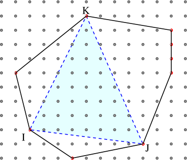
Figure 2: Pictorial representation of the toric formula $c_{IJK}=\frac{N^{2}}{2}\left|\det(k_{I},k_{J},k_{K})\right|$.

5 Field Theory Analysis

From AdS/CFT duality, there are global symmetries $Q_{I}$ and their currents $J_{I}$ on the boundary corresponding to the gauge fields $A^{I}$ in the bulk with the boundary coupling

$$\int d^{4}xA^{I}J_{I}.$$ (5.1)

Thus, the Chern-Simons interaction $c_{IJK}$ in the five-dimensional action induces the triangle anomaly on the CFT side [2]. The numerical coefficient in (2.1) is chosen such that

$$c_{IJK}=\operatorname{tr}(Q_{I}Q_{J}Q_{K})$$ (5.2)

is satisfied. We obtained a concrete supergravity formulae for $c_{IJK}$ in the previous sections. We also know the corresponding quiver theories which flow to CFTs in the IR through recent developments. We will see that the triangle anomaly calculated in the quiver side completely agrees with the supergravity calculation.

5.1 Cubic anomalies from field theories in the toric case

In this section we compute all the cubic ’t Hooft anomalies in the case of gauge theories dual to toric Sasaki-Einstein manifolds. In order to perform this computation, we first have to know the structure of the quiver theory. Although we will summarize below only the facts that we need later, the method of obtaining the quiver gauge theory from the toric data and vice versa is a beautiful subject in itself. It has been known for some time that it can be done in principle algorithmically, but the method was unwieldy and required extensive calculation. Now various works, [32, 33, 11, 12, 13, 18, 34, 35, 36], give a technique to obtain the quiver theory in a much more streamlined way by the so-called dimer methods. They accomplished the most difficult parts at the same time, namely the determination of the superpotential of the quiver theory. We would like the reader to refer to the works cited above for these developments.

We will use the following properties of the quiver gauge theories dual to a toric diagram:

1. The gauge group is $SU(N)^{\mathcal{A}}$, where $\mathcal{A}$ is twice the area of the toric diagram.

2. The bifundamental chiral superfields can be grouped in $d(d-1)/2$ sets, which we can call $\mathcal{B}_{ij}$, where $i$ and $j$ label two external $(p,q)$-legs. In each set $\mathcal{B}_{ij}$ there are

   $$|\mathcal{B}_{ij}|=p_{i}\,q_{j}-p_{j}\,q_{i}$$ (5.3)

   of bifundamental fields, where $(p_{i},q_{i})$ is the $i$-th external $(p,q)$-leg.

3. All the fields belonging to the same set $\mathcal{B}_{ij}$ have, under the global symmetry $U(1)^{d}$, the same charges $Q^{ij}_{I}$.

The full group of global symmetries, as we saw, is

$$U(1)^{d}=U(1)^{3}_{F}\times U(1)_{B}^{d-3}$$ (5.4)

if the toric diagram has $d$ points on the boundary.

Before proceeding let us comment on what is known about the validity of the various properties. Property $1$ is a well established fact. The total number of gauge groups is equal to the total number of compact cycles ($0$-, $2$- and $4$-cycles) in the completely resolved Calabi-Yau. Since there is no odd-homology, this number is the Euler number of the resolved non compact Calabi-Yau, which is, in turn, given by twice the area of the toric diagram. Properties $2$ and $3$ were proposed in [11], under the name of “folded quiver”. Property $2$ was shown for toric del Pezzo surfaces in [37], and there is by now a lot of evidence for it, for instance the exact quiver gauge theories are known for $Y^{p,q}$/$L^{p,q|r}$ and they satisfy property $2$. We expect it to be possible to give a general proof studying intersection numbers of compact three-cycles in the mirror Calabi-Yau, as was conjectured in [11] on the base of [37]. For recent work see [35, 36, 34]. In particular using the procedure devised in [35] it is possible to derive formula (5.3) from the counting of the intersection of $(p,q)$-legs when drawn in the planar torus (again, consult [35] for details). Let us stress that the properties $1$ and $2$ are inherently topological, in the sense that the former depends only on the topology of the Calabi-Yau and the latter that of its mirror. Property $3$ instead goes slightly beyond purely topological properties, for instance the existence of three $U(1)$ flavor symmetries is related to isometries of the Calabi-Yau metric. Let us notice also that in [37] a different interpretation of (5.3) was given, and we now know that the correct interpretation is in terms of property $3$.

Very strong evidence for the validity of all the three properties listed above was given in the work of Butti and Zaffaroni [18, 34], where it was shown that the field theory computation of the cubic ’t Hooft anomaly $c_{RRR}$ matches precisely the geometric results for the volumes of the Sasaki-Einstein, as expected from ${\text{AdS}}/\text{CFT}$ correspondence. The volumes on the gravity side can be computed using the results of Martelli, Sparks and Yau [5], which enables to compute the volumes just in terms of toric data. We will show that all cubic ’t Hooft anomalies $c_{IJK}$ match with the Chern-Simons coefficients as computed from gravity.

As an aside, let us note that, beyond ’t Hooft anomalies, using the “folded quiver” picture, one can readily compute the scaling dimension of dibaryon operators and succesfully match with string theory. This gives additional evidence for the validity of properties $1,2$ and $3$. Also the topology of some SUSY three-cycle can be matched with this picture [12].

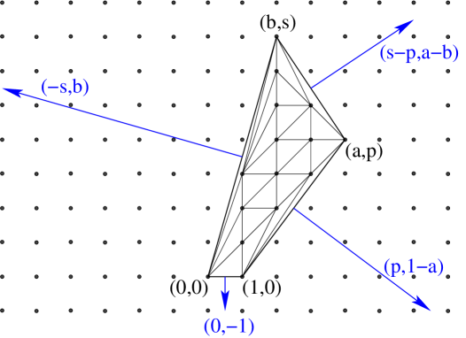
Figure 3: A generic toric diagram with four corners, i.e. a generic $L^{p,q|r}$, and the associated $(p,q)$-web. We have $s=p+q-r$. The integers $a$ and $b$ are such that $as-bp=q$.

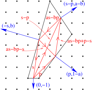
Figure 4: An example of “folded quiver.” From a generic toric diagram with four nodes we can immediately compute the multiplicities of $6$ sets of bifundamental fields.

In order to compute the full set of cubic ’t Hooft anomalies we need to identify the $d$ $U(1)$ global symmetries. We will take all the $d$ symmetries to be $R$-symmetries (taking linear combinations it is obvious how to obtain $d-1$ ordinary $U(1)$ symmetries). There is a natural way to associate a $U(1)$ symmetry to every external node in the toric diagram: the charge of a field under the $i$-th symmetry is one if the $i$-th node on the right of the arrow corresponding to the field in the folded quiver diagram, zero otherwise. For instance external fields in the folded quiver diagram are charged only under one $U(1)$ symmetry. In this way all chiral superfields have charges $0$ or $1$ under the $U(1)^{d}$ global symmetry. The superpotential corresponds to closed loops of the folded quiver. Thus, its charge under the $i$-th $U(1)$ symmetry is $1$. It implies that the commutation relation between $I$-th $U(1)$ charge $Q_{I}$ and the supercharge $Q_{\alpha}$ is $[Q_{I},Q_{\alpha}]=-Q_{\alpha}/2$. This in turn means that the gauginos have thus charge one half and their contribution to cubic anomalies is always $\mathcal{A}N^{2}/8$. Then, the fermionic component of the bifundamental superfields have thus charge $-1/2$ or $1/2$. We thus see that in this way all the charges are half integral, and every bifundamental field contributes $\pm N^{2}/8$ to the cubic anomalies. The point is that this basis is precisely the field theory dual of the basis considered in the previous subsection. Indeed, the dibaryon constructed from the field in $\mathcal{B}_{I,I+1}$ has the charge $\delta_{IJ}N$ under the symmetry $Q_{J}$, which precisely matches the charge of the D3-brane which wraps the cycle $C_{I}$, see (3.4).

Let us report in detail the results for the case of toric diagram with $4$ corners. The charges are given by table 1.

$$\begin{array}[]{|c||c||c|c|c|c||c|c|c|c|}\hline\cr\ \mbox{Field}&\ \mbox{Number}&Q_{1}&\ Q_{2}&\ Q_{3}&\ Q_{4}&\ Q^{F}_{1}&\ Q^{F}_{2}&\ Q^{F}_{3}&\ Q^{F}_{4}\\ \hline\cr\hline\cr\mathcal{B}_{12}&p&1&0&0&0&\phantom{-}1/2&-1/2&-1/2&-1/2\\ \hline\cr\mathcal{B}_{23}&r&0&1&0&0&-1/2&\phantom{-}1/2&-1/2&-1/2\\ \hline\cr\mathcal{B}_{34}&q&0&0&1&0&-1/2&-1/2&\phantom{-}1/2&-1/2\\ \hline\cr\mathcal{B}_{41}&p+q-r&0&0&0&1&-1/2&-1/2&-1/2&\phantom{-}1/2\\ \hline\cr\mathcal{B}_{13}&q-r&1&1&0&0&\phantom{-}1/2&\phantom{-}1/2&-1/2&-1/2\\ \hline\cr\mathcal{B}_{42}&r-p&1&0&0&1&\phantom{-}1/2&-1/2&-1/2&\phantom{-}1/2\\ \hline\cr\text{ Gauge}&p+q&0&0&0&0&\phantom{-}1/2&\phantom{-}1/2&\phantom{-}1/2&\phantom{-}1/2\\ \hline\cr\end{array}$$

Table 1: Charge assignments for the basic superfields in the case of toric diagrams with four corners.

It is straightforward to check that the linear ’t Hooft anomalies vanish, i.e. $\operatorname{tr}(Q_{j})=0$. This has to be the case for any superconformal quiver [38, 39]. A general proof of the vanishing of linear anomalies using the folded quiver picture was given in [18]. Since $(Q^{F}_{i})^{2}=1$, $\operatorname{tr}(Q_{j})=0$ also implies that

$$\operatorname{tr}(Q_{i}^{2}Q_{j})=\operatorname{tr}(Q_{j})=0$$ (5.5)

The remaining cubic ’t Hooft anomalies (recall they are completely symmetric) are easily computed to be

$$\operatorname{tr}(Q_{1}Q_{2}Q_{3}) = \,N^{2}\,r\,/2$$ (5.6)

$$\operatorname{tr}(Q_{2}Q_{3}Q_{4}) = \,N^{2}\,q\,/2$$ (5.7)

$$\operatorname{tr}(Q_{3}Q_{4}Q_{1}) = N^{2}(p+q-r)\,/2$$ (5.8)

$$\operatorname{tr}(Q_{4}Q_{1}Q_{2}) = \,N^{2}\,\,p\,/2$$ (5.9)

It is now straightforward to check that these are proportional to the area of the triangles

$$|\det(k_{I},k_{J},k_{K})|$$ (5.10)

spanned by the corners of the toric diagram of figure 3 or 4. Thus we have shown that, for a toric diagram with four edges, the cubic anomaly $c_{IJK}$ is given by

$$c_{IJK}=\frac{N^{2}}{2}|\det(k_{I},k_{J},k_{K})|,$$ (5.11)

which agrees with the supergravity result (4.17).

This nice result can be proven for a generic toric diagram with arbitrary number of edges, by an easy mathematical induction. We leave the details in the Appendix B.

5.2 del Pezzo surfaces

Now we want to discuss the gauge theories corresponding to the complex cones over smooth Kähler-Einstein surfaces, i.e. del Pezzo surfaces $dP_{n}$ for $3\leq n\leq 8$. The quivers were constructed in [40] for toric del Pezzo surfaces ($dP_{1}$, $dP_{2}$ and $dP_{3}$), and in [37, 41] for the non toric ones, i.e. $dP_{n}$ with $4\leq n\leq 8$. The generic superpotential for $dP_{5}$ and $dP_{6}$ was derived in [42], for $dP_{7}$ and $dP_{8}$ the explicit, generic, superpotential is still not known. In [38, 43], all the baryonic and $R$ charges are explicitly listed for $dP_{n}$ up to $n=6$. It is simple to compute, using these data, the cubic ’t Hooft anomalies and to match with our geometrical findings in sec. 4.2.

In [27], the $R$- and baryonic charges of the dibaryons were analyzed through the framework of the exceptional collections on the del Pezzo surfaces. In particular, it was shown that the triangle anomalies among the R-symmetry and two baryonic symmetries, $\operatorname{tr}(RB_{i}B_{j})$, are proportional to the intersection form of the two-cycles which are perpendicular to the Kähler class of the surface. It is easy to check that our formula in sec. 4.2 naturally reproduces the result of [27].

6 Rolling down among Sasaki-Einstein vacua

The triangle anomalies in the CFT side and the Chern-Simons coefficients of the gravity side showed a remarkable behavior. Namely, for quiver theories for toric Sasaki-Einstein manifolds, the coefficient $c_{IJK}$ is determined solely by the toric data $k_{I,J,K}$ and is independent of other $k_{L}$ for $L\neq I,J,K$ (4.13). We would like to give a heuristic physical interpretation of this fact. The same consideration can be applied to the del Pezzo cases, and its manifestation is (4.10). We concentrate on the toric cases below.

Consider a toric Sasaki-Einstein $X$ whose dual toric diagram has $d$ edges. Each edge $E_{I}$ naturally corresponds to a global symmetry $Q_{I}$ in the quiver theory. There are bifundamental fields $\Phi^{I}$ with charge $\delta_{J}^{I}$ under $Q_{J}$. Then, we can form a dibaryon operator

$$B^{I}=\epsilon_{i_{1}i_{2}\ldots i_{N}}\epsilon^{j_{1}j_{2}\ldots j_{N}}\Phi^{I}{}^{i_{1}}_{j_{1}}\Phi^{I}{}^{i_{2}}_{j_{2}}\cdots\Phi^{I}{}^{i_{N}}_{j_{N}}.$$ (6.1)

It has the charge $N\delta_{J}^{I}$ under $Q_{J}$, which is precisely the charge (3.2) of a D3-brane wrapping the three-cycle determined by $E_{I}$.

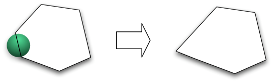
Figure 5: Schematic depiction of the dibaryon condensation. Each edge corresponds to a three-cycle in the toric Sasaki-Einstein around which D3-branes can be wrapped. Higgsing with the corresponding dibaryon operator in the quiver CFT eliminates that edge.

Now, let us give a vacuum expectation value (vev) to $B_{I}$. Since $B_{I}$ is charged only with respect to $Q_{I}$ and not to $Q_{J\neq I}$, the theory flow to a theory with $d-1$ global symmetries. On the gravity side, the Higgsing means that there is an infinite number of D3-branes wrapping around $C_{I}$, which presumably shrinks it just as in the blackhole condensation [44], see figure 5. It is the blowdown of the toric divisor corresponding to $E_{I}$ on the Calabi-Yau cone over $X$. This procedure was used in the determination of the del Pezzo quiver in [41].

Recall that the same triangle anomaly can be calculated either in the ultraviolet or in the infrared. Thus, the triangle anomaly $c_{JKL}$ among the global symmetries other than $Q_{I}$ is the same before and after the Higgsing. Since the Higgsing eliminates the edge $E_{I}$, this means that $c_{JKL}$ is independent of $k_{I}$. One can repeat the flow many times and we can reduce the toric diagram to a triangle, which is an orbifold of $\mathcal{N}=4$ $SU(N)$ super Yang-Mills theory.

Let us consider the behavior of the central charge $a$ along the flow. Consider a flow from the UV quiver theory to the IR quiver theory triggered by giving a vev to $B_{I}$. The IR theory contains also a free chiral scalar field which represents the fluctuation of the vev of $B_{I}$. Its contribution to $a$ is of order $1/N^{2}$ compared to the contribution from the interacting part, so we can neglect them henceforth. Then, from the invariance of $c_{IJK}$ along the flow (4.13), the central charge $a$ in the IR theory can be obtained by maximizing the same function as that for the UV theory in a smaller region. Thus, $a$ will presumably decrease, with the usual caveat on the fact that the trial function attains the maximum only locally.

Let us compare the process we saw in this section with the rolling among Calabi-Yau vacua [45]. There, theories on various topologically-distinct Calabi-Yau manifolds are connected by adiabatically changing the moduli. Here, theories on various topologically-distinct Sasaki-Einstein manifolds are connected by the renormalization-group flow induced by the Higgsing of the dibaryons. Both have the same number of supercharges, and both can be understood as the Higgsing. Thus, we suggest to dub the phenomenon we found as the “rolling among Sasaki-Einstein vacua,” although the rolling is unidirectional.

More detailed analysis of the rolling is clearly necessary and will be interesting. We hope to revisit this problem in the future.

7 Conclusion

In this paper we explored a particular aspect of the ${\text{AdS}}_{5}/\text{CFT}_{4}$ correspondence. Namely, the matching between the Chern-Simons interaction in the five-dimensional bulk and the triangle anomaly in the four-dimensional boundary. More precisely, we derived a formula for the Chern-Simons interactions in terms of three-forms in the Einstein manifold used in the compactification, and we also evaluated the formula for the circle bundles over the del Pezzo surfaces and for the toric Sasaki-Einstein manifolds. Furthermore, we successfully matched the resulting expression to the triangle anomaly from the dual field theory. Condensation of dibaryons was crucial in the physical understanding of the calculation of the triangle anomaly in both sides of the duality.

We also found that the charges of the D-branes wrapping various three-cycles in the Sasaki-Einstein naturally and nontrivially combine the angular momenta along the isometry directions and the baryonic charges.

There are several open problems that we would like to point out. One possible direction of further research is to extend the determination of the lowest-derivatives terms in the AdS theory and to check the very special geometry of the vector multiplet scalars. Another direction will be the study of a more thorough understanding of the charges of D-branes wrapping inside the Sasaki-Einstein manifolds. The new ingredients came in mostly from the fact that the manifold comes with a group action. We made some comments in the appendix C. Finally, the physics of the rolling among the Sasaki-Einstein vacua should be studied more thoroughly. We hope to revisit these problems in the future.

Appendix A Details of supergravity reduction

Our goal in this section is to perform a compactification of a ten-dimensional solution of IIB supergravity to five dimensions. It is worth stressing that we are not attempting a reduction to a five-dimensional theory. In fact, there is an extensive literature on supergravity reduction on positively curved symmetric manifolds. For example, there are some constructions of full consistent non-linear Ansatz for the reduction on the spheres [46]. Other interesting truncations are presented in [47] and references therein. In this subsection we carry out the compactification of Type IIB theory on generic 5-dimensional Einstein manifolds. As such, we are forced to the perturbative analysis and will not pursue full non-linear reduction in this paper. Indeed, it is known that consistent reductions are possible only for a restricted set of manifolds [48].

Consider Type IIB theory compactified on an Einstein 5-manifold $X$ to have a five-dimensional theory on ${\text{AdS}}_{5}$. Let the coordinates of $X$ and AdS be $y^{i}$ and $x^{\mu}$, and their fünfbeine be $e^{i}$ and $f^{\mu}$, respectively.

Since the action of the self-dual five-form in ten dimensions is rather subtle, we carry out the Kaluza-Klein analysis at the level of equation of motion. Let us explain the main technical point before going into the details. Schematically, one first expands the fluctuation using the harmonics of the internal manifold $X$,

$$\phi(x,y)=\phi_{0}(x,y)+\delta\phi^{(i)}(x)\psi_{(i)}(y)+\cdots,$$ (A.1)

so that $\delta\phi^{(i)}$ are the mass eigenstates. Then, one can identify the cubic couplings such as the CS coefficient by finding the equation of motion of $\delta\phi^{(i)}$ in the form

$$(D-m^{2})\delta\phi^{(i)}=C^{(i)}_{(j)(k)}\delta\phi^{(i)}\delta\phi^{(j)}+\cdots.$$ (A.2)

If one is only interested in obtaining certain parts of the cubic coupling, one can set to zero any fluctuation which does not multiply the couplings. It does not change the results, and at the same time it greatly reduces the calculational burden.

Another technical difficulty lies in maintaining the self-duality of the Ansatz for the five-form. Suppose $X$ has $\ell$ $U(1)$ isometries $k_{a}^{i}$, $a=1,\ldots,\ell$ with period $2\pi$. The ansatz for the metric is the usual one,

$$ds^{2}_{X}=\sum_{i}(e^{i}+k_{a}^{i}A^{a})^{2},$$ (A.3)

where $e^{i}$ are the fünfbein forms of the Einstein manifold and $A^{a}=A^{a}_{\mu}dx^{\mu}$ are one-forms on ${\text{AdS}}_{5}$.

Let us abbreviate $\hat{e}^{i}=e^{i}+k_{a}^{i}A^{a}$. Then, the Hodge star exchanges

$$f^{1},\ldots,f^{5}\quad\longleftrightarrow\quad\hat{e}^{1},\ldots,\hat{e}^{5}.$$ (A.4)

Thus, one can anticipate that the introduction of the following $\hat{\phantom{M}}$ operation on differential forms of $X$ defined by replacing $e$ by $\hat{e}$,

$$\alpha^{(p)}=\alpha_{i_{1}\cdots i_{p}}e^{i_{1}}\cdots e^{i_{p}}\mapsto\hat{\alpha}^{(p)}\equiv\alpha_{i_{1}\cdots i_{p}}\hat{e}^{i_{1}}\cdots\hat{e}^{i_{p}},$$ (A.5)

greatly helps in maintaining the self-duality of the Ansatz for $F_{5}$.

The following two formulae are useful in calculation. First is a formula for the $\hat{\phantom{o}}$ operation using interior products:

$$\hat{\alpha}=\alpha+A^{a}\wedge\iota_{k_{a}}\alpha+\frac{1}{2}A^{a}\wedge A^{b}\wedge\iota_{k_{b}}\iota_{k_{a}}\alpha+\cdots.$$ (A.6)

Another is $*(\alpha^{(5-p)}\wedge\beta^{(p)})=(-)^{p}(*\alpha)\wedge*\beta$ where the number in the parentheses in the superscript denotes the degree of the forms.

Let us carry out what we have just outlined. The equations of motion and the Bianchi identity in Type IIB supergravity is:

$$R_{\mu\nu} =\frac{c}{24}F_{\mu....}F_{\nu}{}^{....},$$ (A.7)

$$F =*F,$$ (A.8)

$$dF =0$$ (A.9)

where $R_{\mu\nu}$ is the Ricci curvature of the ten-dimensional metric and $F$ is the self-dual five-form field strength. The right hand side of (A.7) should be contracted in a suitable way. $c$ is a convention dependent constant. We set other form fields and fermions to zero, and dilaton to constant. In the following, we use the following convention when converting a $p$-form $\omega$ into its components $\omega_{\mu_{1}\cdots\mu_{p}}$ by defining

$$\omega=\frac{1}{p!}\omega_{\mu_{1}\mu_{2}\cdots\mu_{p}}dx^{\mu_{1}}dx^{\mu_{2}}\cdots dx^{\mu_{p}}.$$ (A.10)

An example is

$$F=\frac{1}{120}F_{\mu\nu\rho\sigma\tau}dx^{\mu}dx^{\nu}dx^{\rho}dx^{\sigma}dx^{\tau}$$ (A.11)

for the self-dual five-form $F$.

The zero-th order solution is

$$ds^{2} =L^{2}ds^{2}_{{\text{AdS}}}+L^{2}ds^{2}_{X}, F =\frac{2\pi N}{V}\left(\mathrm{vol}_{X}+\mathrm{vol}_{{\text{AdS}}}\right).$$ (A.12)

We take the convention $R_{\mu\nu}=-4g_{\mu\nu}$ for the AdS part, $R_{mn}=4g_{mn}$ for the SE part. Plugging (A.12) in to the equation of motion of the metric, we get

$$4=c\left(\frac{2\pi N}{V}\right)^{2}L^{-8}.$$ (A.13)

Let us expand the fluctuation around the zero-th order solution in modes. One can consistently set to zero all the modes which are not invariant under the $U(1)$ isometries. We then take the ansatz for $F_{5}$ as

$$\frac{V}{2\pi N}F_{5}=\hat{e}^{1}\cdots\hat{e}^{5}+B^{a}\wedge*k_{a}-F^{I}\wedge\hat{\omega}_{I}+*F^{I}\wedge\widehat{*\omega_{I}}+(*B^{a})\wedge k_{a}+f^{1}\cdots f^{5}$$ (A.14)

where $k_{a}=g_{ij}k_{a}^{i}dy^{j}$, $\omega_{I}$ are three-forms to be identified shortly, $B^{a}=B^{a}_{\mu}dx^{\mu}$ and $F^{I}=F^{I}_{\mu\nu}dx^{\mu}dx^{\nu}/2$. We will see that this gives consistent equation of motion in five dimensions. Note that

$$(\omega_{I}\ \text{elsewhere in the article})=-\frac{2\pi}{V}(\omega_{I}\ \text{here}).$$ (A.15)

This definition saves messy factors of powers of $2\pi$.

$F_{5}$ above satisfies $F_{5}=*F_{5}$ by construction, because the one-forms $f^{\mu}$ and $\hat{e}^{i}$ constitutes the zehnbein of the metric. $dF_{5}=0$ requires

$$d\omega_{I}=c^{a}_{I}\iota_{k_{a}}\mathrm{vol}_{X}$$ (A.16)

for some constants $c^{a}_{I}$. We define $k_{I}\equiv c^{a}_{I}k_{a}$ for brevity. Note also that

$$(k_{I}\ \text{elsewhere in the article})=2\pi(k_{I}\ \text{here}).$$ (A.17)

Furthermore, we assume $\omega_{I}$ to be co-closed. Then, $dF_{5}=0$ imposes on $B^{a}$, $F^{I}$ the equations

$$d(A^{a}+B^{a}) =c^{a}_{I}F^{I},$$ (A.18)

$$dF^{I} =0,$$ (A.19)

$$d(*F^{I})\wedge*\omega_{I} =-(*B^{a})\wedge dk_{a}+F^{I}\wedge F^{J}\wedge\iota_{k_{J}}\omega_{I}$$ (A.20)

where we kept the fluctuations up to the second order. Let us define $\omega_{a}$ by $*dk_{a}/8$. One has $d\omega_{a}=\iota_{k^{a}}\mathrm{vol}$ by using the fact that we have $*d*dk=2tk$ for any Killing vector $k$ in an Einstein spaces with $R_{ij}=tg_{ij}$. Then we see, from (A.20),

$$d*F^{I}\wedge\omega_{K}\wedge*\omega_{I}=-8*B^{a}\wedge\omega_{K}\wedge*\omega_{a}+F^{I}\wedge F^{J}\wedge\omega_{K}\wedge\iota_{k_{J}}\omega_{I}.$$ (A.21)

Another important EOM comes from the Ricci curvature $R_{\mu\hat{i}}f^{\mu}\hat{e}^{i}$ with one leg in the AdS and one leg in the SE. While

$$R_{\mu\hat{i}}=\frac{1}{2}k_{ia}\nabla_{\nu}(\partial_{\mu}A^{a}_{\nu}-\partial_{\nu}A^{a}_{\mu})$$ (A.22)

from (A.3), the right hand side of (A.7) is given by

$$\frac{c}{24}F_{\mu....}F_{\hat{i}}{}^{....} =\frac{c}{24}\left(\frac{2\pi N}{V}\right)^{2}L^{-8}\left(48B^{a}_{\mu}k_{ai}-6(*F^{I})_{\mu\nu\rho}(*\omega_{I})_{..}F^{J\nu\rho}(\omega_{J})_{\hat{i}}{}^{..}\right)$$ (A.23)

$$=8B^{a}_{\mu}k_{ai}-4(*F^{I}\wedge F^{J})_{\mu}\frac{(\omega_{I}\iota_{e_{i}}\omega_{J})}{\mathrm{vol}_{X}}.$$ (A.24)

Thus we get

$$\frac{1}{16}(d*dA^{a})\wedge(k_{a}\cdot k_{K})\mathrm{vol}_{X}=\\ *B^{a}\wedge(k_{a}\cdot k_{K})\mathrm{vol}_{X}+\frac{1}{2}F^{I}\wedge F^{J}\wedge\omega_{I}\iota_{k_{K}}\omega_{J}.$$ (A.25)

where we define $(a\cdot b)$ for two one-forms $a=a_{i}dx^{i}$ and $b=b_{i}dx^{i}$ by $(a\cdot b)=a_{i}b_{j}g^{ij}$.

From (A.21) and (A.25) we see $B^{a}$ are the massive eigenmodes under Kaluza-Klein expansion, hence we need to set $B^{a}=0$ to get the Ansatz for the massless fluctuation. Let us add the both sides of the equations (A.21) and (A.25), and integrate over the internal manifold $X$. Using $\int_{X}\omega_{K}\wedge*\omega_{a}=\int_{X}k_{K}k_{a}\mathrm{vol}_{X}/8$, the term including the massive mode $B^{a}$ vanishes, and we finally obtain the EOM for massless fields :

$$d*F^{I}\int_{X}(\omega_{K}\wedge*\omega_{I}+\frac{1}{16}(k_{K}\cdot k_{I})\mathrm{vol}_{X})=\frac{1}{4}F^{I}\wedge F^{J}\int_{X}\omega_{\{I}\wedge\iota_{k_{J}}\omega_{K\}}$$ (A.26)

where $\{IJK\}=IJK+IKJ+\cdots$ without $1/6$. The factor which multiplies $d*dF_{I}$ exactly reproduces the combination $g^{-2}_{IJ}{}^{KK}+g^{-2}_{IJ}{}^{CC}$ which appeared in ref [25], where it was derived in a slightly different way.

Let us recapitulate what happens during the detailed calculation. If we reduce some higher-dimensional form-field theory on an internal manifold without isometries, we need to have simultaneously closed and co-closed wavefunctions in the internal manifold to have a massless field in the non-compact dimensions. If the metric is the sole dynamical field, then upon reduction an isometry produces a gauge field through the ansatz (2.6). Through the coupling between the metric and five-form field, the gauge field from $g_{\mu\nu}$ and the gauge field from $F_{5}$ with co-closed but nonclosed wavefunctions get off-diagonal components in the mass matrix, and precisely one linear combination remains massless for one Killing vector field. Thus, the number of massless gauge fields in AdS is

$$d=\ell+b^{3},$$ (A.27)

where $\ell$ is the number of independent Killing vectors and $b^{3}$ is the dimension of $H^{3}(X)$.

Appendix B Triangle anomaly for general toric quivers

In this appendix we prove the formula

$$c_{IJK}=\frac{N^{2}}{2}|\det(k_{I},k_{J},k_{L})|$$ (B.1)

for quiver gauge theories on the D3-branes probing the tip of a toric Calabi-Yau cone.

Let us denote by $k_{I}=(1,\vec{k}_{I})$ ($I=1,\ldots,d$) the toric data of the toric Calabi-Yau manifold. We set $k_{0}\equiv k_{d}$. One can express the same data using the language of the $(p,q)$-web, in which the direction of the $i$-th external leg is given by $(p_{i},q_{i})=\vec{k}_{i}-\vec{k}_{i-1}$. The field content of the corresponding quiver theory is summarized in sec. 5.1, properties 1, 2 and 3. Let us consider a linear combination $Q=a^{I}Q_{I}$ of the $U(1)$ charges $Q_{I}$. Then, the charge of the superpotential under $Q$ is $\sum a_{I}$ and the charge of the chiral superfields in $\mathcal{B}_{ij}$ is

$$\sum_{K=i}^{j-1}a^{K}=a_{i}+a_{i+1}+\cdots+a_{j-1}.$$ (B.2)

The number $n_{ij}$ of chiral superfields in $\mathcal{B}_{ij}$ is given by the intersection number of the two $(p,q)$-legs, that is,

$$n_{ij}=\det(\vec{k}_{j}-\vec{k}_{j-1},\vec{k}_{i}-\vec{k}_{i-1}),$$ (B.3)

while the number $n_{V}$ of gauge groups is given by the area of the toric diagram

$$n_{V}=\sum\det(\vec{k}_{I}-\vec{k}_{1},\vec{k}_{I+1}-\vec{k}_{1}).$$ (B.4)

Then the triangle anomaly among three $Q$’s is given by

$$\frac{1}{N^{2}}c_{IJK}^{\text{CFT}}a^{I}a^{J}a^{K}=n_{V}(\frac{1}{2}\sum a^{I})^{3}+\sum_{I<J}n_{IJ}\left(\sum_{K=I}^{J-1}a^{K}-\frac{1}{2}\sum a^{I}\right)^{3}.$$ (B.5)

This expression follows from the folded quiver picture of [11], and appeared explicitly in the work of Butti and Zaffaroni [18]. In the usual formula we have $1$ instead of $\sum a^{I}/2$; we would like to have the triangle anomaly including the global symmetry usually fixed by $\sum a^{I}=2$, so we resurrected that combination.

One can show, by mathematical induction, $c_{IJK}^{\text{CFT}}$ only depends on $k_{I,J,K}$ and not on other $k_{L}$ for $L\neq I,J,K$. nor on the number of edges. The proof goes as follows :

Suppose $I,J,K\neq d$ and let us show $c_{IJK}$ is independent of $k_{d}$. Consider two toric data, one is the original set $\{k_{1},k_{2},\cdots,k_{d}\}$ and the other is $\{k_{1},\cdots,k_{d-1}\}$ without $k_{d}$. Let us distinguish various quantities for the latter by adding tilde above, e.g. $\tilde{n}_{V}$ and so on. Then we have two relations

$$n_{I,{d-1}}+n_{I,d}=\tilde{n}_{I,d-1}$$ (B.6)

and

$$n_{V}-n_{d-1,d}=\tilde{n}_{V}.$$ (B.7)

Applying them to the formula (B.5), we obtain

$$c_{IJK}^{\text{CFT}}a^{I}a^{J}a^{K}\big{|}_{a^{N}=0}=\tilde{c}_{IJK}^{\text{CFT}}a^{I}a^{J}a^{K}.$$ (B.8)

Thus, $c_{IJK}$ for $I,J,K\neq d$ is independent of $k_{d}$. Inductively, we can show that $c_{IJK}$ depends only on $k_{I}$, $k_{J}$ and $k_{K}$.

Hence, we can obtain $c_{IJK}^{\text{CFT}}$ by considering the case of a triangle. One can easily show that, in this case,

$$n_{V}=n_{IJ}=n_{JK}=n_{KI}=|\det(k_{I},k_{J},k_{K})|.$$ (B.9)

Plugging in to the formula (B.5), we finally obtain

$$c_{IJK}^{\text{CFT}}=\frac{N^{2}}{2}|\det(k_{I},k_{J},k_{K})|.$$ (B.10)

It precisely agrees with the result from the supergravity analysis (4.17).

Appendix C More on the charge lattice

We would like to elaborate on the mathematics of the structure of the charges of the D3-branes. The case for the toric Sasaki-Einstein manifolds were analyzed in ref. [12] mainly from the point of view of the toric geometry of the cone. We discuss the problem for arbitrary Einstein manifolds.

Let us denote the space of Killing vectors by $N$, which can be identified with the Lie algebra of $U(1)^{\ell}$. It comes with a natural integral structure by stating that $k\in N$ is one of the lattice points if and only if $e^{2\pi k}=id$. Denote the dual space of $N$ by $M$. Integral points of $M$ correspond to representations of $U(1)^{\ell}$. The Reeb vector $R\in N$ is given when we endow $X$ with the Sasaki structure. If $X$ is Sasaki-Einstein, all the toric data $k\in N$ should be on a plane. The plane is given by a distinguished element $P\in M$ as $\langle P,k\rangle=1$ where $P$ is the image of $R$ under the identification $M\simeq N$ induced by the metric.

We deliberately used the letters $M$ and $N$ to evoke the connection with the toric geometry. Indeed they are precisely $M$ and $N$ lattices of the cone over $X$, if $\ell=3$.

We only consider the branes which wrap three-cycles invariant under the action of $U(1)^{\ell}$. As discussed in section 3.1, two cycles are taken to be equivalent if they form the boundaries of an invariant four-chain. Let us call the group of the equivalence classes of such three-cycles as $HG_{3}(X)$ where $G$ stands for Giant Gravitons. We also denote the space of linear combinations of $\omega_{I}$ by $HG^{3}(X)$, where $\omega_{I}$ are closed up to isometry (2.15).

We have an exact sequence

$$0\to H^{3}(X)\to HG^{3}(X)\to N\to 0$$ (C.1)

where the second arrow is just the inclusion, and the third arrow is given by (2.15). The exactness of the sequence is also obvious.

Correspondingly, we also have another exact sequence

$$0\to M\stackrel{{\scriptstyle\iota}}{{\longrightarrow}}HG_{3}(X)\stackrel{{\scriptstyle\pi}}{{\longrightarrow}}H_{3}(X)\to 0$$ (C.2)

where we assumed, as before, that we can take an invariant representative for all $H_{3}(X)$. Then, the third arrow $\pi$ is just loosening of the equivalence relation. The second arrow $\iota$ is a bit tricky to define, so we postpone the discussion to the end of this section. In the toric case, the above sequence can be obtained from the usual sequence [49]

$$0\to M\to\mathrm{Div}_{T}(C(X))\to\mathrm{Pic}(C(X))\to 0.$$ (C.3)

for the cone $C(X)$ over $X$, where $\mathrm{Div}_{T}$ denotes the group of toric divisors and $\mathrm{Pic}$ is the Picard group.

Two exact sequences have a nice physical interpretation. First, the relation between various gauge fields are given by (C.1). $H^{3}(X)$ is the wavefunction for the purely ‘baryonic’ gauge fields, i.e. gauge fields coming from $F_{5}$. The elements of $N$ are the Killing vector fields of $X$, which give rise to the metric Kaluza-Klein gauge field. Formula (C.1) says that the total space of the gauge field is given by combining the metric and $F_{5}$ gauge fields, and that there is generally no gauge fields which come purely from the metric.

Secondly, the sequence (C.2) relates various charges. Namely, $M$ measures the Kaluza-Klein angular momenta, and $H_{3}(X)$ measures the D3-brane charges wrapping various cycles. The fact that $HG_{3}(X)$ is the extension of $H_{3}(X)$ by $M$ tells us that, although we can have excitations with purely Kaluza-Klein momenta and without D-brane charges, e.g. gravitons, generically any states with D-brane i.e. ‘baryonic’ charges also have angular momenta. It also matches nicely with the result in the recent works [21, 22] which studied the BPS states with no baryonic charges and their charge lattice through the analysis of the spectrum of the Laplacian. The states without D-brane charges also appear as the semiclassical strings moving along the null geodesics. The analysis for $Y^{p,q}$ was carried out in ref. [20].

In the literature on the Sasaki-Einstein/Quiver duality, relatively little attention is paid to the $M$ part of the charges and the $N$ part of the gauge fields, so it seems worthwhile to study further.

Let us now come back to the construction of the second arrow $\iota$ in (C.2). Take an integral basis of Killing vectors $v_{a}$, $a=1,\ldots,\ell$ of $N$ and take the dual basis $u^{a}$ in $M$. The basic idea is first to remove subsets $X_{a}$ from $X$ so that $X\setminus X^{a}$ has a trivial $S^{1}$ bundle structure under the action of the vector field $v_{a}$, second to take a section of the bundle with its graph $Z_{a}$, and finally to set $\iota(v_{a})\equiv\partial Z_{a}$.

The bundle structure is non-trivial, thus one cannot take a genuine section. The best one can do is to get a four-chain. Then, the boundary of the four-chain is the desired image under $\iota$. To construct an element $\iota(u^{a})$ in $HG_{3}(X)$ for $u^{a}$, first let us denote by $Y^{a}$ the three-cycle where the Killing vector $v_{a}$ degenerates. Define $B^{a}=(X\setminus Y^{a})/U(1)_{a}$ where $U(1)_{a}$ is generated by $v_{a}$. Then, the orbit of $v_{a}$ determines a genuine $S^{1}$ bundle

$$S^{1}\to X\setminus Y^{a}\stackrel{{\scriptstyle p}}{{\longrightarrow}}B^{a}.$$ (C.4)

Consider the associated vector bundle over $B^{a}$ obtained by the fiber $S^{1}$ by $\mathbb{C}$, and take a generic section of it. Let the zero locus of the section be given by $t^{ai}\gamma^{a}_{i}$ where $\gamma^{a}_{i}$ is a two-dimensional submanifold of $b^{a}$ and $t^{ai}$ is the multiplicity of the zero at $\gamma^{a}_{i}$. Then consider the bundle

$$S^{1}\to X\setminus(Y^{a}\cup\bigcup_{a}p^{-1}(\gamma^{a}_{i}))\to B^{a}\setminus\bigcup_{a}\gamma^{a}_{i}.$$ (C.5)

It is a trivial $S^{1}$ bundle because we removed $\gamma^{a}_{i}$, and we can take a section $Z^{a}$ of it.

Using $Z_{a}$, we define the image of $u^{a}$ by $\iota$ as

$$\iota(u^{a})\equiv\partial Z^{a}=Y^{a}+t^{ai}p^{-1}(\gamma^{a}_{i}).$$ (C.6)

As before, we assume that we can take $Y^{a}$ and $\gamma^{a}_{i}$ to be invariant under isometries.

The exactness of the sequence (C.2) is now obvious because the image is the boundary of the four-chain $Z^{a}$. Secondly, a D3-brane wrapping on $\partial Z^{a}$ has angular momentum $\delta^{a}_{b}$ with respect to the isometry $v_{b}$. It is because

$$\int_{\partial Z^{a}}\omega_{b}=\int_{Z^{a}}d\omega_{b}=\int_{Z^{a}}\iota_{k_{b}}\mathrm{vol}^{\circ}=\delta^{a}_{b}.$$ (C.7)

For the sake of completeness, we would like to describe the second arrow $\iota$ in (C.2) and in (C.3) in the toric case. Let us denote the cone over $X$ by $C(X)$, which is a toric variety. For $u\in M$, we can take a rational function $\chi^{u}$ on $C(X)$ satisfying

$$v^{i}\partial_{i}\chi^{u}=\sqrt{-1}\langle u,v\rangle\chi^{u}$$ (C.8)

for $v\in N$, where $\langle u,v\rangle$ is the natural pairing between $M$ and $N$. It is unique up to multiplication by a complex number, since the torus action is dense in $C(X)$. Then the image is precisely the principal divisor $\mathrm{div}(\chi^{u})$ determined by $\chi^{u}$ restricted on $X$, where the principal divisor $\mathrm{div}(f)$ of a rational function $f$ is

$$\mathrm{div}(f)=\sum_{\alpha}n_{\alpha}C^{\alpha},$$ (C.9)

with $C^{\alpha}$ the loci of the zeros and the poles of $f$ and with $n_{\alpha}$ the degree of zeros or the negative of the degree of poles at $n_{\alpha}$.

References

- [1] J. M. Maldacena, “The large N limit of superconformal field theories and supergravity,” Adv. Theor. Math. Phys. 2 (1998) 231 [Int. J. Theor. Phys. 38 (1999) 1113] [arXiv:hep-th/9711200].
- [2] E. Witten, “Anti-de Sitter space and holography,” Adv. Theor. Math. Phys. 2 (1998) 253 [arXiv:hep-th/9802150].
- [3] M. Pernici, K. Pilch and P. van Nieuwenhuizen, “Gauged Supergravity,” Nucl. Phys. B 259 (1985) 460.
- [4] M. Günaydin, L. J. Romans and N. P. Warner, “Compact and Noncompact Gauged Supergravity Theories in Five-Dimensions,” Nucl. Phys. B 272 (1986) 598.
- [5] D. Martelli, J. Sparks and S. T. Yau, “The geometric dual of -maximisation for toric Sasaki-Einstein manifolds,” arXiv:hep-th/0503183.
- [6] I. R. Klebanov and E. Witten, “Superconformal field theory on threebranes at a Calabi-Yau singularity,” Nucl. Phys. B 536 (1998) 199 [arXiv:hep-th/9807080].
- [7] J. P. Gauntlett, D. Martelli, J. Sparks and D. Waldram, “Sasaki-Einstein metrics on ,” Adv. Theor. Math. Phys. 8 (2004) 711 [arXiv:hep-th/0403002].
- [8] M. Cvetič, H. Lu, D. N. Page and C. N. Pope, “New Einstein-Sasaki spaces in five and higher dimensions,” Phys. Rev. Lett. 95 (2005) 071101 [arXiv:hep-th/0504225].
- [9] D. Martelli and J. Sparks, “Toric Sasaki-Einstein metrics on ,” Phys. Lett. B 621 (2005) 208 [arXiv:hep-th/0505027].
- [10] S. Benvenuti, S. Franco, A. Hanany, D. Martelli and J. Sparks, “An infinite family of superconformal quiver gauge theories with Sasaki-Einstein duals,” JHEP 0506 (2005) 064 [arXiv:hep-th/0411264].
- [11] S. Benvenuti and M. Kruczenski, “From Sasaki-Einstein spaces to quivers via BPS geodesics: ,” JHEP 0604 (2006) 033 [arXiv:hep-th/0505206].
- [12] S. Franco, A. Hanany, D. Martelli, J. Sparks, D. Vegh and B. Wecht, “Gauge theories from toric geometry and brane tilings,” JHEP 0601 (2006) 128 [arXiv:hep-th/0505211].
- [13] A. Butti, D. Forcella and A. Zaffaroni, “The dual superconformal theory for manifolds,” JHEP 0509 (2005) 018 [arXiv:hep-th/0505220].
- [14] D. Anselmi, D. Z. Freedman, M. T. Grisaru and A. A. Johansen, “Nonperturbative formulas for central functions of supersymmetric gauge theories,” Nucl. Phys. B 526 (1998) 543 [arXiv:hep-th/9708042].
- [15] M. Henningson and K. Skenderis, “The holographic Weyl anomaly,” JHEP 9807 (1998) 023 [arXiv:hep-th/9806087].
- [16] S. S. Gubser, “Einstein manifolds and conformal field theories,” Phys. Rev. D 59 (1999) 025006 [arXiv:hep-th/9807164].
- [17] K. Intriligator and B. Wecht, “The exact superconformal -symmetry maximizes ,” Nucl. Phys. B 667 (2003) 183 [arXiv:hep-th/0304128].
- [18] A. Butti and A. Zaffaroni, “-charges from toric diagrams and the equivalence of -maximization and -minimization,” JHEP 0511 (2005) 019 [arXiv:hep-th/0506232].
- [19] M. Bertolini, F. Bigazzi and A. L. Cotrone, “New checks and subtleties for AdS/CFT and -maximization,” JHEP 0412 (2004) 024 [arXiv:hep-th/0411249].
- [20] S. Benvenuti and M. Kruczenski, “Semiclassical strings in Sasaki-Einstein manifolds and long operators in N = 1 gauge theories,” arXiv:hep-th/0505046.
- [21] H. Kihara, M. Sakaguchi and Y. Yasui, “Scalar Laplacian on Sasaki-Einstein manifolds ,” Phys. Lett. B 621 (2005) 288 [arXiv:hep-th/0505259].
- [22] T. Oota and Y. Yasui, “Toric Sasaki-Einstein manifolds and Heun equations,” Nucl. Phys. B 742 (2006) 275 [arXiv:hep-th/0512124].
- [23] F. Canoura, J. D. Edelstein, L. A. Pando Zayas, A. V. Ramallo and D. Vaman, “Supersymmetric branes on x and their field theory duals,” JHEP 0603 (2006) 101 [arXiv:hep-th/0512087].
- [24] Y. Tachikawa, “Five-dimensional supergravity dual of -maximization,” Nucl. Phys. B 733 (2006) 188 [arXiv:hep-th/0507057].
- [25] E. Barnes, E. Gorbatov, K. Intriligator and J. Wright, “Current correlators and AdS/CFT geometry,” Nucl. Phys. B 732 (2006) 89 [arXiv:hep-th/0507146].
- [26] S. Benvenuti, A. Hanany and P. Kazakopoulos, “The toric phases of the quivers,” JHEP 0507 (2005) 021 [arXiv:hep-th/0412279].
- [27] C. P. Herzog and J. Walcher, “Dibaryons from exceptional collections,” JHEP 0309 (2003) 060 [arXiv:hep-th/0306298].
- [28] J. McGreevy, L. Susskind and N. Toumbas, “Invasion of the giant gravitons from anti-de Sitter space,” JHEP 0006 (2000) 008 [arXiv:hep-th/0003075].
- [29] M. T. Grisaru, R. C. Myers and O. Tafjord, “SUSY and Goliath,” JHEP 0008 (2000) 040 [arXiv:hep-th/0008015].
- [30] A. Mikhailov, “Giant gravitons from holomorphic surfaces,” JHEP 0011 (2000) 027 [arXiv:hep-th/0010206].
- [31] C. E. Beasley, “BPS branes from baryons,” JHEP 0211 (2002) 015 [arXiv:hep-th/0207125].
- [32] A. Hanany and K. D. Kennaway, “Dimer models and toric diagrams,” arXiv:hep-th/0503149.
- [33] S. Franco, A. Hanany, K. D. Kennaway, D. Vegh and B. Wecht, “Brane dimers and quiver gauge theories,” JHEP 0601 (2006) 096 [arXiv:hep-th/0504110].
- [34] A. Butti and A. Zaffaroni, “From toric geometry to quiver gauge theory: The equivalence of -maximization and -minimization,” Fortsch. Phys. 54 (2006) 309 [arXiv:hep-th/0512240].
- [35] A. Hanany and D. Vegh, “Quivers, tilings, branes and rhombi,” arXiv:hep-th/0511063.
- [36] B. Feng, Y. H. He, K. D. Kennaway and C. Vafa, “Dimer models from mirror symmetry and quivering amoebae,” arXiv:hep-th/0511287.
- [37] A. Hanany and A. Iqbal, “Quiver theories from D6-branes via mirror symmetry,” JHEP 0204 (2002) 009 [arXiv:hep-th/0108137].
- [38] K. Intriligator and B. Wecht, “Baryon charges in 4D superconformal field theories and their AdS duals,” Commun. Math. Phys. 245 (2004) 407 [arXiv:hep-th/0305046].
- [39] S. Benvenuti and A. Hanany, “New results on superconformal quivers,” JHEP 0604 (2006) 032 [arXiv:hep-th/0411262].
- [40] B. Feng, A. Hanany and Y. H. He, “D-brane gauge theories from toric singularities and toric duality,” Nucl. Phys. B 595 (2001) 165 [arXiv:hep-th/0003085].
- [41] B. Feng, S. Franco, A. Hanany and Y. H. He, “Unhiggsing the del Pezzo,” JHEP 0308 (2003) 058 [arXiv:hep-th/0209228].
- [42] M. Wijnholt, “Large volume perspective on branes at singularities,” Adv. Theor. Math. Phys. 7 (2004) 1117 [arXiv:hep-th/0212021].
- [43] S. Franco, A. Hanany and P. Kazakopoulos, “Hidden exceptional global symmetries in 4d CFTs,” JHEP 0407 (2004) 060 [arXiv:hep-th/0404065].
- [44] B. R. Greene, D. R. Morrison and A. Strominger, “Black hole condensation and the unification of string vacua,” Nucl. Phys. B 451 (1995) 109 [arXiv:hep-th/9504145].
- [45] P. Candelas, P. S. Green and T. Hübsch, “Rolling Among Calabi-Yau Vacua,” Nucl. Phys. B 330 (1990) 49.
- [46] H. Nastase, D. Vaman and P. van Nieuwenhuizen, “Consistency of the reduction and the origin of self-duality in odd dimensions,” Nucl. Phys. B 581 (2000) 179 [arXiv:hep-th/9911238].
- [47] M. Cvetič et al., “Embedding AdS black holes in ten and eleven dimensions,” Nucl. Phys. B 558 (1999) 96 [arXiv:hep-th/9903214].
- [48] P. Hoxha, R. R. Martinez-Acosta and C. N. Pope, “Kaluza-Klein consistency, Killing vectors, and Kähler spaces,” Class. Quant. Grav. 17 (2000) 4207 [arXiv:hep-th/0005172].
- [49] William Fulton, “Introduction to Toric Varieties,” Princeton University Press, Princeton, 1993