Renormalization group dependence of the QCD coupling
G. X. Peng
a b c
Abstract
The general relation between the standard expansion coefficients and
the beta function for the QCD coupling is exactly derived in a
mathematically strict way. It is accordingly found that an infinite
number of logarithmic terms are lost in the standard expansion with
a finite order, and these lost terms can be given in a closed form.
Numerical calculations, by a new matching-invariant coupling with
the corresponding beta function to four-loop level, show that the
new expansion converges much faster.
running coupling, expansion coefficients,
matching-invariant, beta function
pacs: 21.65.+f, 24.85.+p, 12.38.-t, 11.30.Rd
It is of crucial importance to consider the renormalization
group (RG) scale dependence of the strong coupling, in order
to have full consistency in QCD and its applications
Peng2005epl ; Fraga2005prd71 α = α s / π = g 2 / ( 4 π 2 ) 𝛼 subscript 𝛼 𝑠 𝜋 superscript 𝑔 2 4 superscript 𝜋 2 \alpha=\alpha_{s}/\pi=g^{2}/(4\pi^{2})
u d α d u = − ∑ i = 0 ∞ β i α i + 2 ≡ β ( α ) , 𝑢 d 𝛼 d 𝑢 superscript subscript 𝑖 0 subscript 𝛽 𝑖 superscript 𝛼 𝑖 2 𝛽 𝛼 u\frac{\mathrm{d}\alpha}{\mathrm{d}u}=-\sum_{i=0}^{\infty}\beta_{i}\alpha^{i+2}\equiv\beta(\alpha), (1)
where the β 𝛽 \beta Gross1973PRL30.1343 Caswell1974PRL33.244 Tarasov1980PLB93.429 Larin1997PLB400.379 tHooft1973NPB61.455 N f subscript 𝑁 f N_{\mathrm{f}} β i ( N f ) = ∑ j ≥ 0 β i , j N f j . subscript 𝛽 𝑖 subscript 𝑁 f subscript 𝑗 0 subscript 𝛽 𝑖 𝑗
superscript subscript 𝑁 f 𝑗 \beta_{i}(N_{\mathrm{f}})=\sum_{j\geq 0}\beta_{i,j}N_{\mathrm{f}}^{j}.\ β i , j subscript 𝛽 𝑖 𝑗
\beta_{i,j}
[ β i , j ] = [ 11 / 2 − 1 / 3 0 0 51 / 4 − 19 / 12 0 0 2857 64 − 5032 576 325 1728 0 β 3 , 0 β 3 , 1 β 3 , 2 1093 93312 ] delimited-[] subscript 𝛽 𝑖 𝑗
delimited-[] 11 2 1 3 0 0 51 4 19 12 0 0 2857 64 5032 576 325 1728 0 subscript 𝛽 3 0
subscript 𝛽 3 1
subscript 𝛽 3 2
1093 93312 [\beta_{i,j}]=\left[\begin{array}[]{cccc}11/2&-1/3&0&0\\
51/4&-19/12&0&0\\
\frac{2857}{64}&-\frac{5032}{576}&\frac{325}{1728}&0\\
\beta_{3,0}&\beta_{3,1}&\beta_{3,2}&\frac{1093}{93312}\\
\end{array}\right] (2)
with
β 3 , 0 = 891 ζ 3 / 32 + 149753 / 768 ≈ 228.4606573 , β 3 , 1 = − 1627 ζ 3 / 864 − 1078361 / 20736 ≈ − 54.26788763 , β 3 , 2 = 809 ζ 3 / 1296 + 50065 / 20736 ≈ 3.164758128 , formulae-sequence subscript 𝛽 3 0
891 subscript 𝜁 3 32 149753 768 228.4606573 subscript 𝛽 3 1
1627 subscript 𝜁 3 864 1078361 20736 54.26788763 subscript 𝛽 3 2
809 subscript 𝜁 3 1296 50065 20736 3.164758128 \beta_{3,0}=891\zeta_{3}/32+149753/768\approx 228.4606573,\ \beta_{3,1}=-1627\zeta_{3}/864-1078361/20736\approx-54.26788763,\ \beta_{3,2}=809\zeta_{3}/1296+50065/20736\approx 3.164758128, ζ 𝜁 \zeta ζ 2 = π 2 / 6 subscript 𝜁 2 superscript 𝜋 2 6 \zeta_{2}=\pi^{2}/6 ζ 3 ≈ 1.202056903 subscript 𝜁 3 1.202056903 \zeta_{3}\approx 1.202056903 ζ 4 = π 4 / 90 subscript 𝜁 4 superscript 𝜋 4 90 \zeta_{4}=\pi^{4}/90 ζ 5 ≈ 1.036927755 subscript 𝜁 5 1.036927755 \zeta_{5}\approx 1.036927755 N c = 3 subscript 𝑁 c 3 N_{\mathrm{c}}=3 Larin1997PLB400.379 2 2 i + 1 superscript 2 2 𝑖 1 2^{2i+1}
In practical applications, it is convenient to have an explicit expression
of the α 𝛼 \alpha u 𝑢 u L = 1 / ln ( u 2 / Λ 2 ) 𝐿 1 superscript 𝑢 2 superscript Λ 2 L=1/\ln(u^{2}/\Lambda^{2}) Λ Λ \Lambda Eidelman2004PLB592.1 Chetyrkin1997PRL79 ln j L superscript 𝑗 𝐿 \ln^{j}L
To solve Eq. (1
β ´ ( α ) ≡ β 0 2 β 1 [ 1 β ( α ) − β 1 β 0 2 α + 1 β 0 α 2 ] . ´ 𝛽 𝛼 superscript subscript 𝛽 0 2 subscript 𝛽 1 delimited-[] 1 𝛽 𝛼 subscript 𝛽 1 superscript subscript 𝛽 0 2 𝛼 1 subscript 𝛽 0 superscript 𝛼 2 \acute{\beta}(\alpha)\equiv\frac{\beta_{0}^{2}}{\beta_{1}}\left[\frac{1}{\beta(\alpha)}-\frac{\beta_{1}}{\beta_{0}^{2}\alpha}+\frac{1}{\beta_{0}\alpha^{2}}\right]. (3)
With the series expression for β ( α ) 𝛽 𝛼 \beta(\alpha) 1
β ´ ( α ) = ∑ j = 0 ∞ ( β 0 β j + 2 / β 1 − β j + 1 ) α j ∑ i = 0 ∞ β i α i , ´ 𝛽 𝛼 superscript subscript 𝑗 0 subscript 𝛽 0 subscript 𝛽 𝑗 2 subscript 𝛽 1 subscript 𝛽 𝑗 1 superscript 𝛼 𝑗 superscript subscript 𝑖 0 subscript 𝛽 𝑖 superscript 𝛼 𝑖 \acute{\beta}(\alpha)=\frac{\sum_{j=0}^{\infty}(\beta_{0}\beta_{j+2}/\beta_{1}-\beta_{j+1})\alpha^{j}}{\sum_{i=0}^{\infty}\beta_{i}\alpha^{i}}, (4)
which indicates that β ´ ( α ) ´ 𝛽 𝛼 \acute{\beta}(\alpha) α = 0 𝛼 0 \alpha=0
β ´ ( α ) = ∑ k = 0 ∞ β ´ k α k . ´ 𝛽 𝛼 superscript subscript 𝑘 0 subscript ´ 𝛽 𝑘 superscript 𝛼 𝑘 \acute{\beta}(\alpha)=\sum_{k=0}^{\infty}\acute{\beta}_{k}\alpha^{k}. (5)
The expansion coefficients β ´ k subscript ´ 𝛽 𝑘 \acute{\beta}_{k}
β ´ k = 1 k ! d k d α k β ´ ( α ) | α = 0 . subscript ´ 𝛽 𝑘 evaluated-at 1 𝑘 superscript d 𝑘 d superscript 𝛼 𝑘 ´ 𝛽 𝛼 𝛼 0 \acute{\beta}_{k}=\frac{1}{k!}\left.\frac{\mathrm{d}^{k}}{\mathrm{d}\alpha^{k}}\acute{\beta}(\alpha)\right|_{\alpha=0}. (6)
Another easy way to obtain these coefficients is
to use the recursive relation
β ´ k = β k + 2 β 1 − β k + 1 β 0 − 1 β 0 ∑ l = 0 k − 1 β k − l β ´ l , subscript ´ 𝛽 𝑘 subscript 𝛽 𝑘 2 subscript 𝛽 1 subscript 𝛽 𝑘 1 subscript 𝛽 0 1 subscript 𝛽 0 superscript subscript 𝑙 0 𝑘 1 subscript 𝛽 𝑘 𝑙 subscript ´ 𝛽 𝑙 \acute{\beta}_{k}=\frac{\beta_{k+2}}{\beta_{1}}-\frac{\beta_{k+1}}{\beta_{0}}-\frac{1}{\beta_{0}}\sum_{l=0}^{k-1}\beta_{k-l}\acute{\beta}_{l}, (7)
with the obvious initial condition
β ´ 0 = β 2 / β 1 − β 1 / β 0 . subscript ´ 𝛽 0 subscript 𝛽 2 subscript 𝛽 1 subscript 𝛽 1 subscript 𝛽 0 \acute{\beta}_{0}={\beta_{2}}/{\beta_{1}}-{\beta_{1}}/{\beta_{0}}.
Let
L = 1 / ln ( u / Λ ) , 𝐿 1 𝑢 Λ L=1/\ln(u/\Lambda), Λ Λ \Lambda 1 − L 2 d α d L = β ( α ) , superscript 𝐿 2 d 𝛼 d 𝐿 𝛽 𝛼 -L^{2}\frac{\mathrm{d}\alpha}{\mathrm{d}L}=\beta(\alpha), − d L L 2 = d α β ( α ) = [ − 1 β 0 α 2 + β 1 β 0 2 α + β 1 β 0 2 β ´ ( α ) ] d α . d 𝐿 superscript 𝐿 2 d 𝛼 𝛽 𝛼 delimited-[] 1 subscript 𝛽 0 superscript 𝛼 2 subscript 𝛽 1 superscript subscript 𝛽 0 2 𝛼 subscript 𝛽 1 superscript subscript 𝛽 0 2 ´ 𝛽 𝛼 d 𝛼 -\frac{\mathrm{d}L}{L^{2}}=\frac{\mathrm{d}\alpha}{\beta(\alpha)}=\left[-\frac{1}{\beta_{0}\alpha^{2}}+\frac{\beta_{1}}{\beta_{0}^{2}\alpha}+\frac{\beta_{1}}{\beta_{0}^{2}}\acute{\beta}(\alpha)\right]\mathrm{d}\alpha. 1 L − C ′ = 1 β 0 α + β 1 β 0 2 ln α + β 1 β 0 2 ∫ 0 α β ´ ( x ) d x , 1 𝐿 superscript 𝐶 ′ 1 subscript 𝛽 0 𝛼 subscript 𝛽 1 superscript subscript 𝛽 0 2 𝛼 subscript 𝛽 1 superscript subscript 𝛽 0 2 superscript subscript 0 𝛼 ´ 𝛽 𝑥 differential-d 𝑥 \frac{1}{L}-C^{\prime}=\frac{1}{\beta_{0}\alpha}+\frac{\beta_{1}}{\beta_{0}^{2}}\ln\alpha+\frac{\beta_{1}}{\beta_{0}^{2}}\int_{0}^{\alpha}\acute{\beta}(x)\mathrm{d}x,
1 − C ′ L = L β 0 α + β 1 β 0 2 L ln α + β 1 L β 0 2 ∑ k = 1 ∞ β ´ k − 1 k α k , 1 superscript 𝐶 ′ 𝐿 𝐿 subscript 𝛽 0 𝛼 subscript 𝛽 1 superscript subscript 𝛽 0 2 𝐿 𝛼 subscript 𝛽 1 𝐿 superscript subscript 𝛽 0 2 superscript subscript 𝑘 1 subscript ´ 𝛽 𝑘 1 𝑘 superscript 𝛼 𝑘 1-C^{\prime}L=\frac{L}{\beta_{0}\alpha}+\frac{\beta_{1}}{\beta_{0}^{2}}L\ln\alpha+\frac{\beta_{1}L}{\beta_{0}^{2}}\sum_{k=1}^{\infty}\frac{\acute{\beta}_{k-1}}{k}\alpha^{k}, (8)
where C ′ superscript 𝐶 ′ C^{\prime}
Let
α = L β 0 Y ( L ) , 𝛼 𝐿 subscript 𝛽 0 𝑌 𝐿 \alpha=\frac{L}{\beta_{0}}Y(L),
1 Y + L ∗ ln Y + ∑ k = 1 ∞ β ` k L ∗ k + 1 Y k = 1 − C L ∗ − L ∗ ln L , 1 𝑌 superscript 𝐿 𝑌 superscript subscript 𝑘 1 subscript ` 𝛽 𝑘 superscript superscript 𝐿 𝑘 1 superscript 𝑌 𝑘 1 𝐶 superscript 𝐿 superscript 𝐿 𝐿 \frac{1}{Y}+L^{*}\ln Y+\sum_{k=1}^{\infty}\grave{\beta}_{k}{L^{*}}^{k+1}Y^{k}=1-CL^{*}-L^{*}\ln L, (9)
where
L ∗ ≡ ( β 1 / β 0 2 ) L superscript 𝐿 subscript 𝛽 1 superscript subscript 𝛽 0 2 𝐿 L^{*}\equiv(\beta_{1}/\beta_{0}^{2})L C ≡ ( β 0 2 / β 1 ) C ′ − ln β 0 𝐶 superscript subscript 𝛽 0 2 subscript 𝛽 1 superscript 𝐶 ′ subscript 𝛽 0 C\equiv(\beta_{0}^{2}/\beta_{1})C^{\prime}-\ln\beta_{0}
β ` k ≡ 1 k ( β 0 β 1 ) k β ´ k − 1 . subscript ` 𝛽 𝑘 1 𝑘 superscript subscript 𝛽 0 subscript 𝛽 1 𝑘 subscript ´ 𝛽 𝑘 1 \grave{\beta}_{k}\equiv\frac{1}{k}\left(\frac{\beta_{0}}{\beta_{1}}\right)^{k}\acute{\beta}_{k-1}. (10)
The graved beta function β ` k subscript ` 𝛽 𝑘 \grave{\beta}_{k} β ´ k subscript ´ 𝛽 𝑘 \acute{\beta}_{k} 6 7
β ` 1 subscript ` 𝛽 1 \displaystyle\grave{\beta}_{1} = \displaystyle= − 1 + β ˙ 0 β ˙ 2 , β ` 2 = 1 / 2 − β ˙ 0 β ˙ 2 + ( 1 / 2 ) β ˙ 0 2 β ˙ 3 , 1 subscript ˙ 𝛽 0 subscript ˙ 𝛽 2 subscript ` 𝛽 2
1 2 subscript ˙ 𝛽 0 subscript ˙ 𝛽 2 1 2 superscript subscript ˙ 𝛽 0 2 subscript ˙ 𝛽 3 \displaystyle-1+\dot{\beta}_{0}\dot{\beta}_{2},\ \grave{\beta}_{2}=1/2-\dot{\beta}_{0}\dot{\beta}_{2}+(1/2){\dot{\beta}}_{0}^{2}\dot{\beta}_{3}, (11)
β ` 3 subscript ` 𝛽 3 \displaystyle\grave{\beta}_{3} = \displaystyle= − 1 3 + β ˙ 0 β ˙ 2 − 1 3 β ˙ 0 2 ( 2 β ˙ 1 β ˙ 3 + β ˙ 2 2 ) + 1 3 β ˙ 0 3 β ˙ 4 , 1 3 subscript ˙ 𝛽 0 subscript ˙ 𝛽 2 1 3 superscript subscript ˙ 𝛽 0 2 2 subscript ˙ 𝛽 1 subscript ˙ 𝛽 3 superscript subscript ˙ 𝛽 2 2 1 3 superscript subscript ˙ 𝛽 0 3 subscript ˙ 𝛽 4 \displaystyle-\frac{1}{3}+\dot{\beta}_{0}\dot{\beta}_{2}-\frac{1}{3}{\dot{\beta}}_{0}^{2}(2\dot{\beta}_{1}\dot{\beta}_{3}+{\dot{\beta}}_{2}^{2})+\frac{1}{3}\dot{\beta}_{0}^{3}\dot{\beta}_{4}, (12)
β ` k ≥ 4 subscript ` 𝛽 𝑘 4 \displaystyle\grave{\beta}_{k\geq 4} = \displaystyle= ( − 1 ) k k + ( − 1 ) k − 1 β ˙ 0 β ˙ 2 + 1 k ∑ s = 1 k − 4 [ ( − 1 ) s β ˙ 0 k − s − 2 \displaystyle\frac{(-1)^{k}}{k}+(-1)^{k-1}\dot{\beta}_{0}\dot{\beta}_{2}+\frac{1}{k}\sum_{s=1}^{k-4}\Bigg{[}(-1)^{s}{\dot{\beta}_{0}}^{k-s-2} (13)
× ∑ r = 0 2 ( ∏ p = 1 s + r ∑ l p = s + r − p + 1 l p − 1 − 1 ) B l , s ( r ) ∏ q = 0 s + r − 1 β l q − l q + 1 ] \displaystyle\times\sum_{r=0}^{2}\left(\prod_{p=1}^{s+r}\sum_{l_{p}=s+r-p+1}^{l_{p-1}-1}\right)B_{l,s}^{(r)}\prod_{q=0}^{s+r-1}\beta_{l_{q}-l_{q+1}}\Bigg{]}
+ β ˙ 0 k − 2 k [ β ˙ l 0 + ∑ l 1 = 1 k − 2 ( β ˙ l 1 + 1 + β ˙ 2 β ˙ l 1 ) β ˙ l 0 − l 1 \displaystyle+\frac{{\dot{\beta}_{0}}^{k-2}}{k}\Bigg{[}\dot{\beta}_{l_{0}}+\sum_{l_{1}=1}^{k-2}(\dot{\beta}_{l_{1}+1}+\dot{\beta}_{2}\dot{\beta}_{l_{1}})\dot{\beta}_{l_{0}-l_{1}}
+ ∑ l 1 = 2 k − 2 ∑ l 2 = 1 l 1 − 1 β ˙ l 0 − l 1 β ˙ l 1 − l 2 β ˙ l 2 + 2 ] \displaystyle\phantom{+\frac{{\dot{\beta}_{0}}^{k-2}}{k}}+\sum_{l_{1}=2}^{k-2}\sum_{l_{2}=1}^{l_{1}-1}\dot{\beta}_{l_{0}-l_{1}}\dot{\beta}_{l_{1}-l_{2}}\dot{\beta}_{l_{2}+2}\Bigg{]}
− β ˙ 0 k − 1 k ( β ˙ k + ∑ s = 0 k − 2 β ˙ l 0 − s β ˙ s + 2 ) + β ˙ 0 k β ˙ k + 1 k , superscript subscript ˙ 𝛽 0 𝑘 1 𝑘 subscript ˙ 𝛽 𝑘 superscript subscript 𝑠 0 𝑘 2 subscript ˙ 𝛽 subscript 𝑙 0 𝑠 subscript ˙ 𝛽 𝑠 2 superscript subscript ˙ 𝛽 0 𝑘 subscript ˙ 𝛽 𝑘 1 𝑘 \displaystyle-\frac{{\dot{\beta}_{0}}^{k-1}}{k}\left(\dot{\beta}_{k}+\sum_{s=0}^{k-2}\dot{\beta}_{l_{0}-s}\dot{\beta}_{s+2}\right)+\frac{{\dot{\beta}_{0}}^{k}\dot{\beta}_{k+1}}{k},
where
l 0 = k − 1 subscript 𝑙 0 𝑘 1 l_{0}=k-1 B l , s ( 0 ) = β ˙ l s superscript subscript 𝐵 𝑙 𝑠
0 subscript ˙ 𝛽 subscript 𝑙 𝑠 B_{l,s}^{(0)}=\dot{\beta}_{l_{s}} B l , s ( 1 ) = β ˙ l s + 1 + 1 + β ˙ 2 β ˙ l s + 1 superscript subscript 𝐵 𝑙 𝑠
1 subscript ˙ 𝛽 subscript 𝑙 𝑠 1 1 subscript ˙ 𝛽 2 subscript ˙ 𝛽 subscript 𝑙 𝑠 1 B_{l,s}^{(1)}=\dot{\beta}_{l_{s+1}+1}+\dot{\beta}_{2}\dot{\beta}_{l_{s+1}} B l , s ( 2 ) = β ˙ l s + 2 + 2 superscript subscript 𝐵 𝑙 𝑠
2 subscript ˙ 𝛽 subscript 𝑙 𝑠 2 2 B_{l,s}^{(2)}=\dot{\beta}_{l_{s+2}+2} β ˙ i = β i / β 1 subscript ˙ 𝛽 𝑖 subscript 𝛽 𝑖 subscript 𝛽 1 \dot{\beta}_{i}=\beta_{i}/\beta_{1} i = 0 , 1 , 2 , … 𝑖 0 1 2 …
i=0,1,2,\ldots
Now suppose we have a solution of the form
Y ( L ) = ∑ i = 0 ∞ ∑ j = 0 i f i , j L ∗ i ln j L , 𝑌 𝐿 superscript subscript 𝑖 0 superscript subscript 𝑗 0 𝑖 subscript 𝑓 𝑖 𝑗
superscript superscript 𝐿 𝑖 superscript 𝑗 𝐿 Y(L)=\sum_{i=0}^{\infty}\sum_{j=0}^{i}f_{i,j}{L^{*}}^{i}\ln^{j}L, (14)
then
1 Y = 1 f 0 , 0 + ∑ i = 1 ∞ ∑ j = 0 i ( ∑ k = 1 i ( − 1 ) k f 0 , 0 k + 1 ⨆ 1 , 0 k f i , j ) L ∗ i ln j L , 1 𝑌 1 subscript 𝑓 0 0
superscript subscript 𝑖 1 superscript subscript 𝑗 0 𝑖 superscript subscript 𝑘 1 𝑖 superscript 1 𝑘 superscript subscript 𝑓 0 0
𝑘 1 superscript subscript square-union 1 0
𝑘 subscript 𝑓 𝑖 𝑗
superscript superscript 𝐿 𝑖 superscript 𝑗 𝐿 \frac{1}{Y}=\frac{1}{f_{0,0}}+\sum_{i=1}^{\infty}\sum_{j=0}^{i}\left(\sum_{k=1}^{i}\frac{(-1)^{k}}{f_{0,0}^{k+1}}\bigsqcup_{1,0}^{k}f_{i,j}\right){L^{*}}^{i}\ln^{j}L, (15)
L ∗ ln Y = ∑ i = 2 ∞ ∑ j = 0 i − 1 ( ∑ k = 1 i − 1 ( − 1 ) k − 1 k f 0 , 0 k ⨆ 1 , 0 k f i − 1 , j ) L ∗ i ln j L , superscript 𝐿 𝑌 superscript subscript 𝑖 2 superscript subscript 𝑗 0 𝑖 1 superscript subscript 𝑘 1 𝑖 1 superscript 1 𝑘 1 𝑘 superscript subscript 𝑓 0 0
𝑘 superscript subscript square-union 1 0
𝑘 subscript 𝑓 𝑖 1 𝑗
superscript superscript 𝐿 𝑖 superscript 𝑗 𝐿 L^{*}\ln Y=\sum_{i=2}^{\infty}\sum_{j=0}^{i-1}\left(\sum_{k=1}^{i-1}\frac{(-1)^{k-1}}{kf_{0,0}^{k}}\bigsqcup_{1,0}^{k}f_{i-1,j}\right){L^{*}}^{i}\ln^{j}L, (16)
∑ k = 1 ∞ β ` k L ∗ k + 1 Y k = ∑ i = 2 ∞ ∑ j = 0 i − 2 ( ∑ k = 2 i − j β ` k − 1 ⨆ 0 , 0 l − k f i − k , j ) L ∗ i ln j L , superscript subscript 𝑘 1 subscript ` 𝛽 𝑘 superscript superscript 𝐿 𝑘 1 superscript 𝑌 𝑘 superscript subscript 𝑖 2 superscript subscript 𝑗 0 𝑖 2 superscript subscript 𝑘 2 𝑖 𝑗 subscript ` 𝛽 𝑘 1 superscript subscript square-union 0 0
𝑙 𝑘 subscript 𝑓 𝑖 𝑘 𝑗
superscript superscript 𝐿 𝑖 superscript 𝑗 𝐿 \sum_{k=1}^{\infty}\grave{\beta}_{k}{L^{*}}^{k+1}Y^{k}=\sum_{i=2}^{\infty}\sum_{j=0}^{i-2}\left(\sum_{k=2}^{i-j}\grave{\beta}_{k-1}\bigsqcup_{0,0}^{l-k}f_{i-k,j}\right){L^{*}}^{i}\ln^{j}L, (17)
where the square cup operator, ⨆ square-union \bigsqcup 9 f i , j subscript 𝑓 𝑖 𝑗
f_{i,j} u ∗ i ln j u superscript superscript 𝑢 𝑖 superscript 𝑗 𝑢 {u^{*}}^{i}\ln^{j}u ( i , j ) = ( 0 , 0 ) 𝑖 𝑗 0 0 (i,j)=(0,0) ( 1 , 0 ) 1 0 (1,0) ( 1 , 1 ) 1 1 (1,1) f 0 , 0 = 1 , f 1 , 0 = C , f 1 , 1 = 1 . formulae-sequence subscript 𝑓 0 0
1 formulae-sequence subscript 𝑓 1 0
𝐶 subscript 𝑓 1 1
1 f_{0,0}=1,\ f_{1,0}=C,\ f_{1,1}=1. i ≥ 2 𝑖 2 i\geq 2 j = i 𝑗 𝑖 j=i ∑ k = 1 i ( − 1 ) k ⨆ 1 , 0 k f i , i = 0 superscript subscript 𝑘 1 𝑖 superscript 1 𝑘 superscript subscript square-union 1 0
𝑘 subscript 𝑓 𝑖 𝑖
0 \sum_{k=1}^{i}(-1)^{k}\bigsqcup_{1,0}^{k}f_{i,i}=0 f i , i = 1 subscript 𝑓 𝑖 𝑖
1 f_{i,i}=1 i ≥ 2 𝑖 2 i\geq 2 j = i − 1 𝑗 𝑖 1 j=i-1
∑ k = 1 i ( − 1 ) k ⨆ 1 , 0 k f i , i − 1 + ∑ k = 1 i − 1 ( − 1 ) k − 1 k ⨆ 1 , 0 k f i − 1 , i − 1 = 0 superscript subscript 𝑘 1 𝑖 superscript 1 𝑘 superscript subscript square-union 1 0
𝑘 subscript 𝑓 𝑖 𝑖 1
superscript subscript 𝑘 1 𝑖 1 superscript 1 𝑘 1 𝑘 superscript subscript square-union 1 0
𝑘 subscript 𝑓 𝑖 1 𝑖 1
0 \sum_{k=1}^{i}(-1)^{k}\bigsqcup_{1,0}^{k}f_{i,i-1}+\sum_{k=1}^{i-1}\frac{(-1)^{k-1}}{k}\bigsqcup_{1,0}^{k}f_{i-1,i-1}=0 (18)
whose solution is
f i , i − 1 = i C + ∑ l = 1 i − 1 ( i / l − 1 ) . subscript 𝑓 𝑖 𝑖 1
𝑖 𝐶 superscript subscript 𝑙 1 𝑖 1 𝑖 𝑙 1 f_{i,i-1}=iC+\sum_{l=1}^{i-1}\left({i}/{l}-1\right).
For i ≥ 2 𝑖 2 i\geq 2 0 ≤ j ≤ i − 2 0 𝑗 𝑖 2 0\leq j\leq i-2
f i , j subscript 𝑓 𝑖 𝑗
\displaystyle f_{i,j} = \displaystyle= ∑ k = 2 i ( − 1 ) k ⨆ 1 , 0 k f i , j + ∑ k = 1 i − 1 ( − 1 ) k − 1 k ⨆ 1 , 0 k f i − 1 , j superscript subscript 𝑘 2 𝑖 superscript 1 𝑘 superscript subscript square-union 1 0
𝑘 subscript 𝑓 𝑖 𝑗
superscript subscript 𝑘 1 𝑖 1 superscript 1 𝑘 1 𝑘 superscript subscript square-union 1 0
𝑘 subscript 𝑓 𝑖 1 𝑗
\displaystyle\sum_{k=2}^{i}(-1)^{k}\bigsqcup_{1,0}^{k}f_{i,j}+\sum_{k=1}^{i-1}\frac{(-1)^{k-1}}{k}\bigsqcup_{1,0}^{k}f_{i-1,j} (19)
+ ∑ k = 1 i − j − 1 β ` k ⨆ 0 , 0 k f i − k − 1 , j . superscript subscript 𝑘 1 𝑖 𝑗 1 subscript ` 𝛽 𝑘 superscript subscript square-union 0 0
𝑘 subscript 𝑓 𝑖 𝑘 1 𝑗
\displaystyle+\sum_{k=1}^{i-j-1}\grave{\beta}_{k}\bigsqcup_{0,0}^{k}f_{i-k-1,j}.
Please note, there are only terms of f i ′ < i , j ′ < j subscript 𝑓 formulae-sequence superscript 𝑖 ′ 𝑖 superscript 𝑗 ′ 𝑗 f_{i^{\prime}<i,j^{\prime}<j}
f 2 , 0 subscript 𝑓 2 0
\displaystyle f_{2,0} = \displaystyle= C 2 + C + β ` 1 , superscript 𝐶 2 𝐶 subscript ` 𝛽 1 \displaystyle C^{2}+C+\grave{\beta}_{1}, (20)
f 3 , 0 subscript 𝑓 3 0
\displaystyle f_{3,0} = \displaystyle= C 3 + 5 2 C 2 + ( 3 β ` 1 + 1 ) C + β ` 1 + β ` 2 , superscript 𝐶 3 5 2 superscript 𝐶 2 3 subscript ` 𝛽 1 1 𝐶 subscript ` 𝛽 1 subscript ` 𝛽 2 \displaystyle C^{3}+\frac{5}{2}C^{2}+(3\grave{\beta}_{1}+1)C+\grave{\beta}_{1}+\grave{\beta}_{2}, (21)
f 3 , 1 subscript 𝑓 3 1
\displaystyle f_{3,1} = \displaystyle= 3 C 2 + 5 C + 3 β ` 1 + 1 , 3 superscript 𝐶 2 5 𝐶 3 subscript ` 𝛽 1 1 \displaystyle 3C^{2}+5C+3\grave{\beta}_{1}+1, (22)
f 4 , 0 subscript 𝑓 4 0
\displaystyle f_{4,0} = \displaystyle= C 4 + ( 13 / 3 ) C 3 + ( 6 β ` 1 + 9 / 2 ) C 2 superscript 𝐶 4 13 3 superscript 𝐶 3 6 subscript ` 𝛽 1 9 2 superscript 𝐶 2 \displaystyle C^{4}+(13/3)C^{3}+(6\grave{\beta}_{1}+9/2)C^{2} (23)
+ ( 1 + 7 A 1 + 4 β ` 2 ) C + 2 β ` 1 2 + Σ i = 1 3 β ` i , 1 7 subscript 𝐴 1 4 subscript ` 𝛽 2 𝐶 2 superscript subscript ` 𝛽 1 2 superscript subscript Σ 𝑖 1 3 subscript ` 𝛽 𝑖 \displaystyle+(1+7A_{1}+4\grave{\beta}_{2})C+2\grave{\beta}_{1}^{2}+\Sigma_{i=1}^{3}\grave{\beta}_{i},
f 4 , 1 subscript 𝑓 4 1
\displaystyle f_{4,1} = \displaystyle= 4 C 3 + 13 C 2 + ( 12 β ` 1 + 9 ) C 4 superscript 𝐶 3 13 superscript 𝐶 2 12 subscript ` 𝛽 1 9 𝐶 \displaystyle 4C^{3}+13C^{2}+(12\grave{\beta}_{1}+9)C (24)
+ 7 A 1 + 4 β ` 2 + 1 , 7 subscript 𝐴 1 4 subscript ` 𝛽 2 1 \displaystyle+7A_{1}+4\grave{\beta}_{2}+1,
f 4 , 2 subscript 𝑓 4 2
\displaystyle f_{4,2} = \displaystyle= 6 C 2 + 13 C + 6 β ` 1 + 9 / 2 , 6 superscript 𝐶 2 13 𝐶 6 subscript ` 𝛽 1 9 2 \displaystyle 6C^{2}+13C+6\grave{\beta}_{1}+9/2, (25)
⋯ ⋯ \displaystyle\cdots
These correspond to the standard form in Ref. Eidelman2004PLB592.1 Chetyrkin1997PRL79
α ( u ) 𝛼 𝑢 \displaystyle\alpha(u) = \displaystyle= 1 β 0 ln ( u / Λ ) { 1 − β 1 ln ln ( u / Λ ) β 0 2 ln ( u / Λ ) \displaystyle\frac{1}{\beta_{0}\ln(u/\Lambda)}\left\{1-\frac{\beta_{1}\ln\ln(u/\Lambda)}{\beta_{0}^{2}\ln(u/\Lambda)}\right. (26)
+ β 1 2 β 0 4 ln 2 ( u / Λ ) [ ( ln ln u Λ − 1 2 ) 2 + β 0 β 2 β 1 2 − 5 4 ] superscript subscript 𝛽 1 2 superscript subscript 𝛽 0 4 superscript 2 𝑢 Λ delimited-[] superscript 𝑢 Λ 1 2 2 subscript 𝛽 0 subscript 𝛽 2 superscript subscript 𝛽 1 2 5 4 \displaystyle\left.+\frac{\beta_{1}^{2}}{\beta_{0}^{4}\ln^{2}(u/\Lambda)}\left[\left(\ln\ln\frac{u}{\Lambda}-\frac{1}{2}\right)^{2}+\frac{\beta_{0}\beta_{2}}{\beta_{1}^{2}}-\frac{5}{4}\right]\right.
− β 1 3 β 0 6 ln 3 ( u / Λ ) [ ( ln ln u Λ − 5 6 ) 3 − β 0 2 β 3 2 β 1 3 + 233 216 \displaystyle\left.-\frac{\beta_{1}^{3}}{\beta_{0}^{6}\ln^{3}(u/\Lambda)}\left[\left(\ln\ln\frac{u}{\Lambda}-\frac{5}{6}\right)^{3}-\frac{\beta_{0}^{2}\beta_{3}}{2\beta_{1}^{3}}+\frac{233}{216}\right.\right.
+ ( 3 β 0 b 2 β 1 2 − 49 12 ) ln ln u Λ ] } . \displaystyle\phantom{-\frac{\beta_{1}^{3}}{\beta_{0}^{6}\ln^{3}(u/\Lambda)}[}+\left(3\frac{\beta_{0}b_{2}}{\beta_{1}^{2}}-\frac{49}{12}\right)\ln\ln\frac{u}{\Lambda}\Bigg{]}\Bigg{\}}.
To give a general representation for the expansion coefficients f i , j subscript 𝑓 𝑖 𝑗
f_{i,j} β ¯ i subscript ¯ 𝛽 𝑖 \bar{\beta}_{i}
β ¯ i = ∑ k = 1 i − 1 [ K ( ⨆ 1 k + 1 β ¯ i − ⨆ 1 k β ¯ i − 1 ) + β ` k ⨆ 0 k β ¯ i − k − 1 ] , subscript ¯ 𝛽 𝑖 superscript subscript 𝑘 1 𝑖 1 delimited-[] 𝐾 superscript subscript square-union 1 𝑘 1 subscript ¯ 𝛽 𝑖 superscript subscript square-union 1 𝑘 subscript ¯ 𝛽 𝑖 1 subscript ` 𝛽 𝑘 superscript subscript square-union 0 𝑘 subscript ¯ 𝛽 𝑖 𝑘 1 \displaystyle\bar{\beta}_{i}=\sum_{k=1}^{i-1}\left[K\left(\bigsqcup_{1}^{k+1}\bar{\beta}_{i}-\bigsqcup_{1}^{k}\bar{\beta}_{i-1}\right)\right.\left.+\grave{\beta}_{k}\bigsqcup_{0}^{k}\bar{\beta}_{i-k-1}\right], (27)
where
K ≡ ( − 1 ) k − 1 ( 1 + 1 / k ) 𝐾 superscript 1 𝑘 1 1 1 𝑘 K\equiv(-1)^{k-1}(1+1/k) β ¯ 0 = 1 subscript ¯ 𝛽 0 1 \bar{\beta}_{0}=1 β ¯ 1 = C subscript ¯ 𝛽 1 𝐶 \bar{\beta}_{1}=C β ¯ i subscript ¯ 𝛽 𝑖 \bar{\beta}_{i} 27 C = 0 𝐶 0 C=0
β ¯ 0 subscript ¯ 𝛽 0 \displaystyle\bar{\beta}_{0} = \displaystyle= 1 , β ¯ 1 = 0 , β ¯ 2 = β ` 1 , β ¯ 3 = β ` 1 + β ` 2 , formulae-sequence 1 subscript ¯ 𝛽 1
0 formulae-sequence subscript ¯ 𝛽 2 subscript ` 𝛽 1 subscript ¯ 𝛽 3 subscript ` 𝛽 1 subscript ` 𝛽 2 \displaystyle 1,\ \bar{\beta}_{1}=0,\ \bar{\beta}_{2}=\grave{\beta}_{1},\ \bar{\beta}_{3}=\grave{\beta}_{1}+\grave{\beta}_{2}, (28)
β ¯ 4 subscript ¯ 𝛽 4 \displaystyle\bar{\beta}_{4} = \displaystyle= ∑ i = 1 3 β ` i + 2 β ` 1 2 , β ¯ 5 = ∑ i = 1 4 β ` i + 9 2 β ` 1 2 + 5 β ` 1 β ` 2 , superscript subscript 𝑖 1 3 subscript ` 𝛽 𝑖 2 superscript subscript ` 𝛽 1 2 subscript ¯ 𝛽 5
superscript subscript 𝑖 1 4 subscript ` 𝛽 𝑖 9 2 superscript subscript ` 𝛽 1 2 5 subscript ` 𝛽 1 subscript ` 𝛽 2 \displaystyle\sum_{i=1}^{3}\grave{\beta}_{i}+2\grave{\beta}_{1}^{2},\ \bar{\beta}_{5}=\sum_{i=1}^{4}\grave{\beta}_{i}+\frac{9}{2}\grave{\beta}_{1}^{2}+5\grave{\beta}_{1}\grave{\beta}_{2}, (29)
β ¯ 6 subscript ¯ 𝛽 6 \displaystyle\bar{\beta}_{6} = \displaystyle= Σ i = 1 5 β ` i + 15 2 β ` 1 2 + 3 β ` 2 2 + 11 β ` 1 β ` 2 + 5 β ` 1 3 , superscript subscript Σ 𝑖 1 5 subscript ` 𝛽 𝑖 15 2 superscript subscript ` 𝛽 1 2 3 superscript subscript ` 𝛽 2 2 11 subscript ` 𝛽 1 subscript ` 𝛽 2 5 superscript subscript ` 𝛽 1 3 \displaystyle\Sigma_{i=1}^{5}\grave{\beta}_{i}+\frac{15}{2}\grave{\beta}_{1}^{2}+3\grave{\beta}_{2}^{2}+11\grave{\beta}_{1}\grave{\beta}_{2}+5\grave{\beta}_{1}^{3},
⋯ ⋯ \displaystyle\cdots
Please note, even when one sets all β i > 2 subscript 𝛽 𝑖 2 \beta_{i>2} β ¯ k > 2 subscript ¯ 𝛽 𝑘 2 \bar{\beta}_{k>2} f i , j subscript 𝑓 𝑖 𝑗
f_{i,j}
It is found that f i , j subscript 𝑓 𝑖 𝑗
f_{i,j}
f i , j = ∑ k = 0 i − j f i − j , k ∑ l = 0 j ( i − l ) ! ( i − j ) ! ( j − l ) ! ⨆ 0 k Φ l , subscript 𝑓 𝑖 𝑗
superscript subscript 𝑘 0 𝑖 𝑗 subscript 𝑓 𝑖 𝑗 𝑘
superscript subscript 𝑙 0 𝑗 𝑖 𝑙 𝑖 𝑗 𝑗 𝑙 superscript subscript square-union 0 𝑘 subscript Φ 𝑙 f_{i,j}=\sum_{k=0}^{i-j}f_{i-j,k}\sum_{l=0}^{j}\frac{(i-l)!}{(i-j)!(j-l)!}\bigsqcup_{0}^{k}\Phi_{l}, (31)
where
⨆ 0 k Φ l superscript subscript square-union 0 𝑘 subscript Φ 𝑙 \bigsqcup_{0}^{k}\Phi_{l} ln k ( 1 + x ) superscript 𝑘 1 𝑥 \ln^{k}(1+x) ln k ( 1 + x ) = ∑ l = 0 ∞ ( ⨆ 0 k Φ l ) x l = ( ∑ l = 0 ∞ Φ l x l ) k = ( ∑ l = 1 ∞ 1 l x l ) k . superscript 𝑘 1 𝑥 superscript subscript 𝑙 0 superscript subscript square-union 0 𝑘 subscript Φ 𝑙 superscript 𝑥 𝑙 superscript superscript subscript 𝑙 0 subscript Φ 𝑙 superscript 𝑥 𝑙 𝑘 superscript superscript subscript 𝑙 1 1 𝑙 superscript 𝑥 𝑙 𝑘 \ln^{k}(1+x)=\sum_{l=0}^{\infty}\left(\bigsqcup_{0}^{k}\Phi_{l}\right)x^{l}=\left(\sum_{l=0}^{\infty}\Phi_{l}x^{l}\right)^{k}=\left(\sum_{l=1}^{\infty}\frac{1}{l}x^{l}\right)^{k}. Φ 0 = 0 , Φ l ≥ 1 = 1 / l , ⨆ 0 0 Φ l = δ l , 0 , ⨆ 0 k Φ 0 = δ k , 0 , ⨆ 0 1 Φ l = Φ l , formulae-sequence subscript Φ 0 0 formulae-sequence subscript Φ 𝑙 1 1 𝑙 formulae-sequence superscript subscript square-union 0 0 subscript Φ 𝑙 subscript 𝛿 𝑙 0
formulae-sequence superscript subscript square-union 0 𝑘 subscript Φ 0 subscript 𝛿 𝑘 0
superscript subscript square-union 0 1 subscript Φ 𝑙 subscript Φ 𝑙 \Phi_{0}=0,\ \Phi_{l\geq 1}=1/l,\ \bigsqcup_{0}^{0}\Phi_{l}=\delta_{l,0},\ \bigsqcup_{0}^{k}\Phi_{0}=\delta_{k,0},\ \bigsqcup_{0}^{1}\Phi_{l}=\Phi_{l},
⨆ 0 k ≥ 2 Φ l ≥ 1 = ( ∏ s = 1 k − 1 ∑ p s = 1 l − k + s − Σ q = 1 k − 1 p q ) 1 l − Σ q = 1 k − 1 p q ∏ s = 1 k − 1 1 p s . superscript subscript square-union 0 𝑘 2 subscript Φ 𝑙 1 superscript subscript product 𝑠 1 𝑘 1 superscript subscript subscript 𝑝 𝑠 1 𝑙 𝑘 𝑠 superscript subscript Σ 𝑞 1 𝑘 1 subscript 𝑝 𝑞 1 𝑙 superscript subscript Σ 𝑞 1 𝑘 1 subscript 𝑝 𝑞 superscript subscript product 𝑠 1 𝑘 1 1 subscript 𝑝 𝑠 \bigsqcup_{0}^{k\geq 2}\Phi_{l\geq 1}=\left(\prod_{s=1}^{k-1}\sum_{p_{s}=1}^{l-k+s-\Sigma_{q=1}^{k-1}p_{q}}\right)\frac{1}{l-\Sigma_{q=1}^{k-1}p_{q}}\prod_{s=1}^{k-1}\frac{1}{p_{s}}. (32)
One can naturally consider to prove Eq. (31 f i , j subscript 𝑓 𝑖 𝑗
f_{i,j}
f i , j = ∑ k = 0 i − j P j , k ( i ) β ¯ k , subscript 𝑓 𝑖 𝑗
superscript subscript 𝑘 0 𝑖 𝑗 superscript subscript 𝑃 𝑗 𝑘
𝑖 subscript ¯ 𝛽 𝑘 f_{i,j}=\sum_{k=0}^{i-j}P_{j,k}^{(i)}\bar{\beta}_{k}, (33)
where P j , k ( i ) superscript subscript 𝑃 𝑗 𝑘
𝑖 P_{j,k}^{(i)} 31 k = i − j 𝑘 𝑖 𝑗 k=i-j k = i − j − 1 𝑘 𝑖 𝑗 1 k=i-j-1
P j , i − j ( i ) = i ! j ! ( i − j ) ! , P j , i − j − 1 ( i ) = i − j ( i − j ) ! ∑ l = 1 j ( i − l ) ! ( j − l ) ! l . formulae-sequence superscript subscript 𝑃 𝑗 𝑖 𝑗
𝑖 𝑖 𝑗 𝑖 𝑗 superscript subscript 𝑃 𝑗 𝑖 𝑗 1
𝑖 𝑖 𝑗 𝑖 𝑗 superscript subscript 𝑙 1 𝑗 𝑖 𝑙 𝑗 𝑙 𝑙 P_{j,i-j}^{(i)}=\frac{i!}{j!(i-j)!},\ P_{j,i-j-1}^{(i)}=\frac{i-j}{(i-j)!}\sum_{l=1}^{j}\frac{(i-l)!}{(j-l)!l}. (34)
Generally for k = i − j − l 𝑘 𝑖 𝑗 𝑙 k=i-j-l l = i − j − k 𝑙 𝑖 𝑗 𝑘 l=i-j-k
P j , k ( i ) superscript subscript 𝑃 𝑗 𝑘
𝑖 \displaystyle P_{j,k}^{(i)} = \displaystyle= 𝒬 ( i , j , l ) 𝒬 ( i − j , l , 0 ) 𝒬 𝑖 𝑗 𝑙 𝒬 𝑖 𝑗 𝑙 0 \displaystyle\mathcal{Q}(i,j,l)\mathcal{Q}(i-j,l,0) (35)
+ ∑ r = 1 l − 1 { ( ∏ p = 1 r ∑ s p = 1 l − 1 − Σ q = 1 p − 1 s q ) [ 𝒬 ( i , j , s 1 ) \displaystyle+\sum_{r=1}^{l-1}\Bigg{\{}\left(\prod_{p=1}^{r}\,\sum_{s_{p}=1}^{l-1-\Sigma_{q=1}^{p-1}s_{q}}\right)\Big{[}\mathcal{Q}(i,j,s_{1})
× 𝒬 ( i − j − Σ q = 1 r − 1 s q , s r , l − Σ q = 1 r s q ) absent 𝒬 𝑖 𝑗 superscript subscript Σ 𝑞 1 𝑟 1 subscript 𝑠 𝑞 subscript 𝑠 𝑟 𝑙 superscript subscript Σ 𝑞 1 𝑟 subscript 𝑠 𝑞 \displaystyle\times\mathcal{Q}\left(i-j-\Sigma_{q=1}^{r-1}s_{q},s_{r},l-\Sigma_{q=1}^{r}s_{q}\right)
× 𝒬 ( i − j − Σ q = 1 r s q , l − Σ q = 1 r s q , 0 ) absent 𝒬 𝑖 𝑗 superscript subscript Σ 𝑞 1 𝑟 subscript 𝑠 𝑞 𝑙 superscript subscript Σ 𝑞 1 𝑟 subscript 𝑠 𝑞 0 \displaystyle\times\mathcal{Q}\left(i-j-\Sigma_{q=1}^{r}s_{q},l-\Sigma_{q=1}^{r}s_{q},0\right)
× ∏ p = 1 r − 1 𝒬 ( i − j − Σ q = 1 p − 1 s q , s p , s p + 1 ) ] } , \displaystyle\times\prod_{p=1}^{r-1}\mathcal{Q}\left(i-j-\Sigma_{q=1}^{p-1}s_{q},s_{p},s_{p+1}\right)\Big{]}\Bigg{\}},
where 𝒬 𝒬 \mathcal{Q}
𝒬 ( i , j , k ) ≡ 1 ( i − j ) ! ∑ l = 0 j ( i − l ) ! ( j − l ) ! ⨆ 0 k Φ l . 𝒬 𝑖 𝑗 𝑘 1 𝑖 𝑗 superscript subscript 𝑙 0 𝑗 𝑖 𝑙 𝑗 𝑙 superscript subscript square-union 0 𝑘 subscript Φ 𝑙 \mathcal{Q}(i,j,k)\equiv\frac{1}{(i-j)!}\sum_{l=0}^{j}\frac{(i-l)!}{(j-l)!}\bigsqcup_{0}^{k}\Phi_{l}. (36)
For a given i 𝑖 i P ( i ) = [ P j , k ( i ) ] superscript 𝑃 𝑖 delimited-[] superscript subscript 𝑃 𝑗 𝑘
𝑖 P^{(i)}=\left[P_{j,k}^{(i)}\right] i + 1 𝑖 1 i+1 P i , k ≥ i − j ( i ) = 0 , P 0 , k ( i ) = δ k , i , P 1 , k ( i ) = k + 1 , P i , k ( i ) = δ k , 0 , P i − 1 , 0 ( i ) = ∑ s = 1 i − 1 ( i / s − 1 ) , P i − 1 , 1 ( i ) = i . formulae-sequence superscript subscript 𝑃 𝑖 𝑘
𝑖 𝑗 𝑖 0 formulae-sequence superscript subscript 𝑃 0 𝑘
𝑖 subscript 𝛿 𝑘 𝑖
formulae-sequence superscript subscript 𝑃 1 𝑘
𝑖 𝑘 1 formulae-sequence superscript subscript 𝑃 𝑖 𝑘
𝑖 subscript 𝛿 𝑘 0
formulae-sequence superscript subscript 𝑃 𝑖 1 0
𝑖 superscript subscript 𝑠 1 𝑖 1 𝑖 𝑠 1 superscript subscript 𝑃 𝑖 1 1
𝑖 𝑖 P_{i,k\geq i-j}^{(i)}=0,\ P_{0,k}^{(i)}=\delta_{k,i},\ P_{1,k}^{(i)}=k+1,\ P_{i,k}^{(i)}=\delta_{k,0},\ P_{i-1,0}^{(i)}=\sum_{s=1}^{i-1}(i/s-1),\ P_{i-1,1}^{(i)}=i. P ( i ) superscript 𝑃 𝑖 P^{(i)} i 𝑖 i
P ( 0 ) = [ 1 ] , P ( 1 ) = [ 0 1 1 0 ] , P ( 2 ) = [ 0 0 1 1 2 0 1 0 0 ] , formulae-sequence superscript 𝑃 0 delimited-[] 1 formulae-sequence superscript 𝑃 1 delimited-[] 0 1 1 0 superscript 𝑃 2 delimited-[] 0 0 1 1 2 0 1 0 0 \displaystyle P^{(0)}=[1],\ P^{(1)}=\left[\begin{array}[]{cc}0&1\\
1&0\end{array}\right],\ P^{(2)}=\left[\begin{array}[]{ccc}0&0&1\\
1&2&0\\
1&0&0\end{array}\right], (42)
P ( 3 ) = [ 0 0 0 1 1 2 3 0 5 2 3 0 0 1 0 0 0 ] , P ( 4 ) = [ 0 0 0 0 1 1 2 3 4 0 9 / 2 7 6 0 0 13 / 3 4 0 0 0 1 0 0 0 0 ] . formulae-sequence superscript 𝑃 3 delimited-[] 0 0 0 1 1 2 3 0 5 2 3 0 0 1 0 0 0 superscript 𝑃 4 delimited-[] 0 0 0 0 1 1 2 3 4 0 9 2 7 6 0 0 13 3 4 0 0 0 1 0 0 0 0 \displaystyle P^{(3)}=\left[\begin{array}[]{cccc}0&0&0&1\\
1&2&3&0\\
\frac{5}{2}&3&0&0\\
1&0&0&0\end{array}\right],\ P^{(4)}=\left[\begin{array}[]{ccccc}0&0&0&0&1\\
1&2&3&4&0\\
{9}/{2}&7&6&0&0\\
{13}/{3}&4&0&0&0\\
1&0&0&0&0\end{array}\right]. (52)
In the traditional minimum subtraction scheme (MS ¯ ¯ MS \overline{\mathrm{MS}} α ( u ) 𝛼 𝑢 \alpha(u) u 𝑢 u MS ¯ ¯ MS \overline{\mathrm{MS}}
Suppose the new coupling α ′ superscript 𝛼 ′ \alpha^{\prime} α 𝛼 \alpha
α ′ = ∑ i = 0 ∞ a i α i + 1 . superscript 𝛼 ′ superscript subscript 𝑖 0 subscript 𝑎 𝑖 superscript 𝛼 𝑖 1 \alpha^{\prime}=\sum_{i=0}^{\infty}a_{i}\alpha^{i+1}. (53)
Then, using the matching condition
α ˇ = ∑ j = 0 ∞ C j α j + 1 ˇ 𝛼 superscript subscript 𝑗 0 subscript 𝐶 𝑗 superscript 𝛼 𝑗 1 \check{\alpha}=\sum_{j=0}^{\infty}C_{j}\alpha^{j+1} Chetyrkin1997PRL79 ; Rodrigo1993PLB313
C 0 subscript 𝐶 0 \displaystyle C_{0} = \displaystyle= 1 , C 1 = 0 , C 2 = 11 / 72 , formulae-sequence 1 subscript 𝐶 1
0 subscript 𝐶 2 11 72 \displaystyle 1,\ \ C_{1}=0,\ \ C_{2}=11/72, (54)
C 3 subscript 𝐶 3 \displaystyle C_{3} = \displaystyle= 575263 124416 − 82043 27648 ζ 3 − 2633 31104 N f , ⋯ 575263 124416 82043 27648 subscript 𝜁 3 2633 31104 subscript 𝑁 f ⋯
\displaystyle\frac{575263}{124416}-\frac{82043}{27648}\zeta_{3}-\frac{2633}{31104}N_{\mathrm{f}},\ \cdots (55)
one has
α ′ ˇ = ∑ i = 0 ∞ [ ∑ k = 0 i a ˇ k ⨆ 0 k + 1 C i − k ] α i + 1 , ˇ superscript 𝛼 ′ superscript subscript 𝑖 0 delimited-[] superscript subscript 𝑘 0 𝑖 subscript ˇ 𝑎 𝑘 superscript subscript square-union 0 𝑘 1 subscript 𝐶 𝑖 𝑘 superscript 𝛼 𝑖 1 \check{\alpha^{\prime}}=\sum_{i=0}^{\infty}\left[\sum_{k=0}^{i}\check{a}_{k}\bigsqcup_{0}^{k+1}C_{i-k}\right]\alpha^{i+1}, (56)
where an overhead check means decreasing N f subscript 𝑁 f N_{\mathrm{f}} N f − 1 subscript 𝑁 f 1 N_{\mathrm{f}}-1 α 𝛼 \alpha α ˇ ′ = α ′ superscript ˇ 𝛼 ′ superscript 𝛼 ′ \check{\alpha}^{\prime}=\alpha^{\prime}
a i = ∑ k = 0 i a ˇ k ⨆ 0 k + 1 C i − k . subscript 𝑎 𝑖 superscript subscript 𝑘 0 𝑖 subscript ˇ 𝑎 𝑘 superscript subscript square-union 0 𝑘 1 subscript 𝐶 𝑖 𝑘 a_{i}=\sum_{k=0}^{i}\check{a}_{k}\bigsqcup_{0}^{k+1}C_{i-k}. (57)
Assume
a i = ∑ j = 0 i a i , j N f j , subscript 𝑎 𝑖 superscript subscript 𝑗 0 𝑖 subscript 𝑎 𝑖 𝑗
superscript subscript 𝑁 f 𝑗 a_{i}=\sum_{j=0}^{i}a_{i,j}N_{\mathrm{f}}^{j}, a ˇ k = ∑ j = 0 k a k , j ( N f − 1 ) j subscript ˇ 𝑎 𝑘 superscript subscript 𝑗 0 𝑘 subscript 𝑎 𝑘 𝑗
superscript subscript 𝑁 f 1 𝑗 \check{a}_{k}=\sum_{j=0}^{k}a_{k,j}(N_{\mathrm{f}}-1)^{j} 57
∑ k = 0 i [ a i , k N f k − ( ⨆ 0 k + 1 C i − k ) ∑ j = 0 k a k , j ( N f − 1 ) j ] = 0 , superscript subscript 𝑘 0 𝑖 delimited-[] subscript 𝑎 𝑖 𝑘
superscript subscript 𝑁 f 𝑘 superscript subscript square-union 0 𝑘 1 subscript 𝐶 𝑖 𝑘 superscript subscript 𝑗 0 𝑘 subscript 𝑎 𝑘 𝑗
superscript subscript 𝑁 f 1 𝑗 0 \sum_{k=0}^{i}\left[a_{i,k}N_{\mathrm{f}}^{k}-\left(\bigsqcup_{0}^{k+1}C_{i-k}\right)\sum_{j=0}^{k}a_{k,j}(N_{\mathrm{f}}-1)^{j}\right]=0, (58)
whose solution is
a 0 subscript 𝑎 0 \displaystyle a_{0} = \displaystyle= a 0 , 0 , a 1 = a 1 , 0 , a 2 = a 2 , 0 + 11 72 a 0 , 0 N f , formulae-sequence subscript 𝑎 0 0
subscript 𝑎 1
subscript 𝑎 1 0
subscript 𝑎 2 subscript 𝑎 2 0
11 72 subscript 𝑎 0 0
subscript 𝑁 f \displaystyle a_{0,0},\ \ a_{1}=a_{1,0},\ \ a_{2}=a_{2,0}+\frac{11}{72}a_{0,0}N_{\mathrm{f}}, (59)
a 3 subscript 𝑎 3 \displaystyle a_{3} = \displaystyle= a 3 , 0 + [ ( 7037 1536 + 82043 27648 ζ 3 ) a 0 , 0 + 11 36 a 1 , 0 ] N f subscript 𝑎 3 0
delimited-[] 7037 1536 82043 27648 subscript 𝜁 3 subscript 𝑎 0 0
11 36 subscript 𝑎 1 0
subscript 𝑁 f \displaystyle a_{3,0}+\left[\left(\frac{7037}{1536}+\frac{82043}{27648}\zeta_{3}\right)a_{0,0}+\frac{11}{36}a_{1,0}\right]N_{\mathrm{f}} (60)
− 2633 62208 a 0 , 0 N f 2 , ⋯ 2633 62208 subscript 𝑎 0 0
superscript subscript 𝑁 f 2 ⋯
\displaystyle-\frac{2633}{62208}a_{0,0}N_{\mathrm{f}}^{2},\ \ \cdots
To definitely fix the new coupling, one needs to choose a i , 0 subscript 𝑎 𝑖 0
a_{i,0} a i , 0 = δ i , 0 . subscript 𝑎 𝑖 0
subscript 𝛿 𝑖 0
a_{i,0}=\delta_{i,0}.
a 0 = 1 , a 1 = 0 , a 2 = ( 11 / 72 ) N f , formulae-sequence subscript 𝑎 0 1 formulae-sequence subscript 𝑎 1 0 subscript 𝑎 2 11 72 subscript 𝑁 f \displaystyle a_{0}=1,\ \ a_{1}=0,\ \ a_{2}=(11/72)N_{\mathrm{f}}, (61)
a 3 = a 3 , 1 N f − 2633 62208 N f 2 , ⋯ subscript 𝑎 3 subscript 𝑎 3 1
subscript 𝑁 f 2633 62208 superscript subscript 𝑁 f 2 ⋯
\displaystyle a_{3}=a_{3,1}N_{\mathrm{f}}-\frac{2633}{62208}N_{\mathrm{f}}^{2},\ \ \cdots (62)
where
a 3 , 1 = 7037 / 1536 + 82043 ζ 3 / 27648 ≈ 8.148377983 . subscript 𝑎 3 1
7037 1536 82043 subscript 𝜁 3 27648 8.148377983 a_{3,1}=7037/1536+82043\zeta_{3}/27648\approx 8.148377983.
α ′ = α + 11 72 N f α 3 + ( a 3 , 1 − 2633 62208 N f ) N f α 4 + ⋯ superscript 𝛼 ′ 𝛼 11 72 subscript 𝑁 f superscript 𝛼 3 subscript 𝑎 3 1
2633 62208 subscript 𝑁 f subscript 𝑁 f superscript 𝛼 4 ⋯ \alpha^{\prime}=\alpha+\frac{11}{72}N_{\mathrm{f}}\alpha^{3}+\left(a_{3,1}-\frac{2633}{62208}N_{\mathrm{f}}\right)N_{\mathrm{f}}\alpha^{4}+\cdots (63)
The renormalization equation for α ′ superscript 𝛼 ′ \alpha^{\prime}
u d α ′ d u = − ∑ i = 0 ∞ β i ′ α ′ i + 2 . 𝑢 d superscript 𝛼 ′ d 𝑢 superscript subscript 𝑖 0 superscript subscript 𝛽 𝑖 ′ superscript superscript 𝛼 ′ 𝑖 2 u\frac{\mathrm{d}\alpha^{\prime}}{\mathrm{d}u}=-\sum_{i=0}^{\infty}\beta_{i}^{\prime}{\alpha^{\prime}}^{i+2}. (64)
The primed beta function β i ′ superscript subscript 𝛽 𝑖 ′ \beta_{i}^{\prime} u d d u 𝑢 d d 𝑢 u\frac{\mathrm{d}}{\mathrm{d}u} 53 64 1 ∑ k = 0 i [ β k ′ ⨆ 0 k + 2 a i − k − ( k + 1 ) a k β i − k ] = 0 , superscript subscript 𝑘 0 𝑖 delimited-[] superscript subscript 𝛽 𝑘 ′ superscript subscript square-union 0 𝑘 2 subscript 𝑎 𝑖 𝑘 𝑘 1 subscript 𝑎 𝑘 subscript 𝛽 𝑖 𝑘 0 \sum_{k=0}^{i}\left[\beta_{k}^{\prime}\bigsqcup_{0}^{k+2}a_{i-k}-(k+1)a_{k}\beta_{i-k}\right]=0, β i ′ superscript subscript 𝛽 𝑖 ′ \beta_{i}^{\prime}
β i ′ = ∑ k = 0 i ( k + 1 ) a k β i − k − ∑ k = 0 i − 1 β k ′ ⨆ 0 k + 1 a i − k . superscript subscript 𝛽 𝑖 ′ superscript subscript 𝑘 0 𝑖 𝑘 1 subscript 𝑎 𝑘 subscript 𝛽 𝑖 𝑘 superscript subscript 𝑘 0 𝑖 1 superscript subscript 𝛽 𝑘 ′ superscript subscript square-union 0 𝑘 1 subscript 𝑎 𝑖 𝑘 \beta_{i}^{\prime}=\sum_{k=0}^{i}(k+1)a_{k}\beta_{i-k}-\sum_{k=0}^{i-1}\beta_{k}^{\prime}\bigsqcup_{0}^{k+1}a_{i-k}. (65)
On application of Eqs. (61 62
β 0 ′ superscript subscript 𝛽 0 ′ \displaystyle\beta_{0}^{\prime} = \displaystyle= β 0 = 11 / 2 − N f / 3 , subscript 𝛽 0 11 2 subscript 𝑁 f 3 \displaystyle\beta_{0}=11/2-N_{\mathrm{f}}/3, (66)
β 1 ′ superscript subscript 𝛽 1 ′ \displaystyle\beta_{1}^{\prime} = \displaystyle= β 1 = 51 / 4 − ( 19 / 12 ) N f , subscript 𝛽 1 51 4 19 12 subscript 𝑁 f \displaystyle\beta_{1}=51/4-(19/12)N_{\mathrm{f}}, (67)
β 2 ′ superscript subscript 𝛽 2 ′ \displaystyle\beta_{2}^{\prime} = \displaystyle= β 2 + a 2 β 0 − a 1 ( β 1 + a 1 β 0 ) subscript 𝛽 2 subscript 𝑎 2 subscript 𝛽 0 subscript 𝑎 1 subscript 𝛽 1 subscript 𝑎 1 subscript 𝛽 0 \displaystyle\beta_{2}+a_{2}\beta_{0}-a_{1}(\beta_{1}+a_{1}\beta_{0}) (68)
= \displaystyle= 2857 64 − 4549 576 N f + 79 576 N f 2 , 2857 64 4549 576 subscript 𝑁 f 79 576 superscript subscript 𝑁 f 2 \displaystyle\frac{2857}{64}-\frac{4549}{576}N_{\mathrm{f}}+\frac{79}{576}N_{\mathrm{f}}^{2},
β 3 ′ superscript subscript 𝛽 3 ′ \displaystyle\beta_{3}^{\prime} = \displaystyle= β 3 + 2 a 3 β 0 − 2 a 1 β 2 + a 1 2 β 1 + 4 a 1 3 β 0 − 6 a 1 a 2 β 0 subscript 𝛽 3 2 subscript 𝑎 3 subscript 𝛽 0 2 subscript 𝑎 1 subscript 𝛽 2 superscript subscript 𝑎 1 2 subscript 𝛽 1 4 superscript subscript 𝑎 1 3 subscript 𝛽 0 6 subscript 𝑎 1 subscript 𝑎 2 subscript 𝛽 0 \displaystyle\beta_{3}+2a_{3}\beta_{0}-2a_{1}\beta_{2}+a_{1}^{2}\beta_{1}+4a_{1}^{3}\beta_{0}-6a_{1}a_{2}\beta_{0}
= \displaystyle= β 3 ( 0 ) + β 3 ( 1 ) N f + β 3 ( 2 ) N f 2 + 10085 186624 N f 3 , superscript subscript 𝛽 3 0 superscript subscript 𝛽 3 1 subscript 𝑁 f superscript subscript 𝛽 3 2 superscript subscript 𝑁 f 2 10085 186624 superscript subscript 𝑁 f 3 \displaystyle\beta_{3}^{(0)}+\beta_{3}^{(1)}N_{\mathrm{f}}+\beta_{3}^{(2)}N_{\mathrm{f}}^{2}+\frac{10085}{186624}N_{\mathrm{f}}^{3},
⋯ ⋯ \displaystyle\cdots
with
β 3 ( 0 ) = 149753 / 768 + ( 891 / 32 ) ζ 3 ≈ 228.4606573 superscript subscript 𝛽 3 0 149753 768 891 32 subscript 𝜁 3 228.4606573 \beta_{3}^{(0)}=149753/768+(891/32)\zeta_{3}\approx 228.4606573 β 3 ( 1 ) = 2118091 / 82944 + ( 2603291 / 55296 ) ζ 3 ≈ 82.12826576 superscript subscript 𝛽 3 1 2118091 82944 2603291 55296 subscript 𝜁 3 82.12826576 \beta_{3}^{(1)}=2118091/82944+(2603291/55296)\zeta_{3}\approx 82.12826576 β 3 ( 2 ) = − 4027 / 1296 − ( 194353 / 82944 ) ζ 3 ≈ − 5.923892810 superscript subscript 𝛽 3 2 4027 1296 194353 82944 subscript 𝜁 3 5.923892810 \beta_{3}^{(2)}=-4027/1296-(194353/82944)\zeta_{3}\approx-5.923892810
It should be mentioned that a different expression for β 2 ′ superscript subscript 𝛽 2 ′ \beta_{2}^{\prime} Marciano1984PRD29 C 2 subscript 𝐶 2 C_{2} Bernreuther1982NPB197
As an application of the general relation between f i , j subscript 𝑓 𝑖 𝑗
f_{i,j}
α = ∑ i = 0 ∞ β 0 β 1 L ∗ i + 1 ∑ j = 0 i f i , j ln j L ≡ ∑ i = 0 ∞ J i . 𝛼 superscript subscript 𝑖 0 subscript 𝛽 0 subscript 𝛽 1 superscript superscript 𝐿 𝑖 1 superscript subscript 𝑗 0 𝑖 subscript 𝑓 𝑖 𝑗
superscript 𝑗 𝐿 superscript subscript 𝑖 0 subscript 𝐽 𝑖 \alpha=\sum_{i=0}^{\infty}\frac{\beta_{0}}{\beta_{1}}{L^{*}}^{i+1}\sum_{j=0}^{i}f_{i,j}\ln^{j}L\equiv\sum_{i=0}^{\infty}J_{i}. (70)
Representing the terms in this expansion with the corresponding
coefficients f i , j subscript 𝑓 𝑖 𝑗
f_{i,j}
[ f i , j ] = [ 1 0 0 0 0 f 1 , 0 1 0 0 0 f 2 , 0 f 2 , 1 1 0 0 ⋮ f 3 , 0 f 3 , 1 f 3 , 2 1 0 f 4 , 0 f 4 , 1 f 4 , 2 f 4 , 3 1 ⋯ ] . delimited-[] subscript 𝑓 𝑖 𝑗
delimited-[] 1 0 0 0 0 missing-subexpression missing-subexpression subscript 𝑓 1 0
1 0 0 0 missing-subexpression missing-subexpression subscript 𝑓 2 0
subscript 𝑓 2 1
1 0 0 ⋮ missing-subexpression subscript 𝑓 3 0
subscript 𝑓 3 1
subscript 𝑓 3 2
1 0 missing-subexpression missing-subexpression subscript 𝑓 4 0
subscript 𝑓 4 1
subscript 𝑓 4 2
subscript 𝑓 4 3
1 missing-subexpression missing-subexpression missing-subexpression missing-subexpression ⋯ missing-subexpression missing-subexpression missing-subexpression missing-subexpression [f_{i,j}]=\left[\begin{array}[]{ccccccc}1&0&0&0&0&\\
f_{1,0}&1&0&0&0&\\
f_{2,0}&f_{2,1}&1&0&0&\vdots\\
f_{3,0}&f_{3,1}&f_{3,2}&1&0&\\
f_{4,0}&f_{4,1}&f_{4,2}&f_{4,3}&1&\\
\phantom{xxxx}&\phantom{xxxx}&\cdots&\phantom{xxxx}&\phantom{xxxx}&\phantom{xxx}\end{array}\right]. (71)
The standard expansion corresponds to summing the terms row by row.
When one takes the expansion to a finite order, i.e., replacing
the ∞ \infty 70 N 𝑁 N f j , j ( N < j < ∞ ) subscript 𝑓 𝑗 𝑗
𝑁 𝑗 f_{j,j}\ (N<j<\infty) f j + 1 , j subscript 𝑓 𝑗 1 𝑗
f_{j+1,j} f j + k , j subscript 𝑓 𝑗 𝑘 𝑗
f_{j+k,j} 0 < j < ∞ 0 𝑗 0<j<\infty k 𝑘 k β 0 ≤ l ≤ k − 2 subscript 𝛽 0 𝑙 𝑘 2 \beta_{0\leq l\leq k-2} f j + k , j subscript 𝑓 𝑗 𝑘 𝑗
f_{j+k,j} j > N 𝑗 𝑁 j>N β i > 2 subscript 𝛽 𝑖 2 \beta_{i>2}
To include the contribution from the terms just mentioned,
we can consider to sum over diagonals,
which can be achieved by taking i = j + k 𝑖 𝑗 𝑘 i=j+k 70
α = β 0 β 1 ∑ k = 0 ∞ ∑ j = 0 ∞ f j + k , j ( L ∗ ln L ) j L ∗ k + 1 ≡ ∑ k = 0 ∞ I k , 𝛼 subscript 𝛽 0 subscript 𝛽 1 superscript subscript 𝑘 0 superscript subscript 𝑗 0 subscript 𝑓 𝑗 𝑘 𝑗
superscript superscript 𝐿 𝐿 𝑗 superscript superscript 𝐿 𝑘 1 superscript subscript 𝑘 0 subscript 𝐼 𝑘 \alpha=\frac{\beta_{0}}{\beta_{1}}\sum_{k=0}^{\infty}\sum_{j=0}^{\infty}f_{j+k,j}\left(L^{*}\ln L\right)^{j}{L^{*}}^{k+1}\equiv\sum_{k=0}^{\infty}I_{k}, (72)
where the expressions for f j + k , j subscript 𝑓 𝑗 𝑘 𝑗
f_{j+k,j} 33
f j , j subscript 𝑓 𝑗 𝑗
\displaystyle f_{j,j} = \displaystyle= 1 , f j + 1 , j = ∑ l = 1 j ( j + 1 l − 1 ) + ( j + 1 ) C , 1 subscript 𝑓 𝑗 1 𝑗
superscript subscript 𝑙 1 𝑗 𝑗 1 𝑙 1 𝑗 1 𝐶 \displaystyle 1,\ \ f_{j+1,j}=\sum_{l=1}^{j}\left(\frac{j+1}{l}-1\right)+(j+1)C, (73)
f j + 2 , j subscript 𝑓 𝑗 2 𝑗
\displaystyle f_{j+2,j} = \displaystyle= β ¯ 2 2 ( j + 1 ) ( j + 2 ) + ( C + 1 2 ) ∑ s = 0 j − 1 ( s + 1 ) ( s + 2 ) j − s subscript ¯ 𝛽 2 2 𝑗 1 𝑗 2 𝐶 1 2 superscript subscript 𝑠 0 𝑗 1 𝑠 1 𝑠 2 𝑗 𝑠 \displaystyle\frac{\bar{\beta}_{2}}{2}(j+1)(j+2)+\left(C+\frac{1}{2}\right)\sum_{s=0}^{j-1}\frac{(s+1)(s+2)}{j-s} (74)
+ 1 2 ∑ s = 0 j − 2 ∑ r = 1 j − s − 1 ( s + 1 ) ( s + 2 ) r ( j − s − r ) , ⋯ 1 2 superscript subscript 𝑠 0 𝑗 2 superscript subscript 𝑟 1 𝑗 𝑠 1 𝑠 1 𝑠 2 𝑟 𝑗 𝑠 𝑟 ⋯
\displaystyle+\frac{1}{2}\sum_{s=0}^{j-2}\sum_{r=1}^{j-s-1}\frac{(s+1)(s+2)}{r(j-s-r)},\ \cdots
From these expressions, we can give compact form to I k subscript 𝐼 𝑘 I_{k}
I 0 subscript 𝐼 0 \displaystyle I_{0} = \displaystyle= L β 0 ∑ j = 0 ∞ ( L ∗ ln L ) j = L / β 0 1 − L ∗ ln L ≡ β 0 X , 𝐿 subscript 𝛽 0 superscript subscript 𝑗 0 superscript superscript 𝐿 𝐿 𝑗 𝐿 subscript 𝛽 0 1 superscript 𝐿 𝐿 subscript 𝛽 0 𝑋 \displaystyle\frac{L}{\beta_{0}}\sum_{j=0}^{\infty}(L^{*}\ln L)^{j}=\frac{L/\beta_{0}}{1-L^{*}\ln L}\equiv\beta_{0}X, (75)
I 1 subscript 𝐼 1 \displaystyle I_{1} = \displaystyle= β 0 β 1 X 2 [ C − ln x ] , subscript 𝛽 0 subscript 𝛽 1 superscript 𝑋 2 delimited-[] 𝐶 𝑥 \displaystyle\beta_{0}\beta_{1}X^{2}\left[C-\ln x\right], (76)
I 2 subscript 𝐼 2 \displaystyle I_{2} = \displaystyle= β 0 β 1 2 X 3 [ f 2 , 0 − f 2 , 1 ln x + ln 2 x ] , subscript 𝛽 0 superscript subscript 𝛽 1 2 superscript 𝑋 3 delimited-[] subscript 𝑓 2 0
subscript 𝑓 2 1
𝑥 superscript 2 𝑥 \displaystyle\beta_{0}\beta_{1}^{2}X^{3}\left[f_{2,0}-f_{2,1}\ln x+\ln^{2}x\right], (77)
where
x ≡ 1 + ( β 1 / β 0 2 ) ln ln ( u / Λ ) / ln ( u / Λ ) , and X ≡ L ∗ / ( β 1 x ) = 1 / [ β 0 2 ln ( u / Λ ) + β 1 ln ln ( u / Λ ) ] . formulae-sequence 𝑥 1 subscript 𝛽 1 superscript subscript 𝛽 0 2 𝑢 Λ 𝑢 Λ and 𝑋 superscript 𝐿 subscript 𝛽 1 𝑥 1 delimited-[] superscript subscript 𝛽 0 2 𝑢 Λ subscript 𝛽 1 𝑢 Λ x\equiv 1+(\beta_{1}/\beta_{0}^{2})\ln\ln(u/\Lambda)/\ln(u/\Lambda),\ \mbox{and}\ X\equiv L^{*}/(\beta_{1}x)=1/[\beta_{0}^{2}\ln(u/\Lambda)+\beta_{1}\ln\ln(u/\Lambda)].
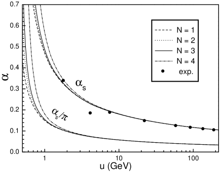
Figure 1:
The QCD coupling as functions of the t’Hooft
unit of mass. The dot, dash, solid, and dot-dash lines are,
respectively, for the order N 𝑁 N Λ Λ \Lambda Λ Λ \Lambda τ 𝜏 \tau Υ Υ \Upsilon + e- event shapes at 22 GeV from the JADE data,
shapes at TRISTAN at 58 GeV, Z width, and e+ e-
event shapes at 135 and 189 GeV.
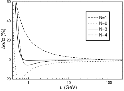
Figure 2:
The relative difference between the new expansion in Eq. (78 70
In Eq. (72 ln j x superscript 𝑗 𝑥 \ln^{j}x I k subscript 𝐼 𝑘 I_{k} α = ∑ k = 0 N I k 𝛼 superscript subscript 𝑘 0 𝑁 subscript 𝐼 𝑘 \alpha=\sum_{k=0}^{N}I_{k} I k subscript 𝐼 𝑘 I_{k} 75 77 Bass2002PRD68 I k subscript 𝐼 𝑘 I_{k}
α = ∑ k = 0 ∞ β 0 β 1 k X k + 1 ∑ l = 0 k ( − 1 ) l f k , l ln l x . 𝛼 superscript subscript 𝑘 0 subscript 𝛽 0 superscript subscript 𝛽 1 𝑘 superscript 𝑋 𝑘 1 superscript subscript 𝑙 0 𝑘 superscript 1 𝑙 subscript 𝑓 𝑘 𝑙
superscript 𝑙 𝑥 \alpha=\sum_{k=0}^{\infty}\beta_{0}\beta_{1}^{k}X^{k+1}\sum_{l=0}^{k}(-1)^{l}f_{k,l}\ln^{l}x. (78)
In Eqs. (78 70 Λ Λ \Lambda C 𝐶 C 64 1 C = 0 𝐶 0 C=0 Bardeen1978PRD18 α ( m Z ) = 0.1187 / π 𝛼 subscript 𝑚 Z 0.1187 𝜋 \alpha(m_{\mathrm{Z}})=0.1187/\pi M Z = 91.1876 subscript 𝑀 Z 91.1876 M_{\mathrm{Z}}=91.1876 C = 0 𝐶 0 C=0 Λ Λ \Lambda Λ 6 subscript Λ 6 \Lambda_{6} Λ 5 subscript Λ 5 \Lambda_{5} Λ 4 subscript Λ 4 \Lambda_{4} Λ 3 subscript Λ 3 \Lambda_{3} u > m t 𝑢 subscript 𝑚 𝑡 u>m_{t} m b < u < m t subscript 𝑚 𝑏 𝑢 subscript 𝑚 𝑡 m_{b}<u<m_{t} m c < u < m b subscript 𝑚 𝑐 𝑢 subscript 𝑚 𝑏 m_{c}<u<m_{b} m s < u < m c subscript 𝑚 𝑠 𝑢 subscript 𝑚 𝑐 m_{s}<u<m_{c} m t = 175 subscript 𝑚 𝑡 175 m_{t}=175 m b = 4.2 subscript 𝑚 𝑏 4.2 m_{b}=4.2 m c = 1.2 subscript 𝑚 𝑐 1.2 m_{c}=1.2 m s = 100 subscript 𝑚 𝑠 100 m_{s}=100
In Fig. 1 78 N 𝑁 N N 𝑁 N 70 78 70 2 u 𝑢 u
Table 1:
QCD renormalization group scale parameter Λ Λ \Lambda Λ i subscript Λ 𝑖 \Lambda_{i} 78 70
Λ Λ \Lambda
Λ 6 subscript Λ 6 \Lambda_{6} Λ 5 subscript Λ 5 \Lambda_{5} Λ 4 subscript Λ 4 \Lambda_{4} Λ 3 subscript Λ 3 \Lambda_{3}
N = 1 𝑁 1 N=1 88
45
208
91
286
124
325
147
N = 2 𝑁 2 N=2 91
95
217
235
303
335
350
377
N = 3 𝑁 3 N=3 90
90
214
212
298
294
340
334
N = 4 𝑁 4 N=4 88
86
209
207
295
291
344
342
To compare the convergence speed of Eqs. (78 70 Λ i subscript Λ 𝑖 \Lambda_{i} i = 3 𝑖 3 i=3 6 6 6 1 Λ i subscript Λ 𝑖 \Lambda_{i} 78 70 78 70 N = 1 𝑁 1 N=1 Λ i subscript Λ 𝑖 \Lambda_{i} 78
α = β 0 β 0 2 ln ( u / Λ ) + β 1 ln ln ( u / Λ ) . 𝛼 subscript 𝛽 0 superscript subscript 𝛽 0 2 𝑢 Λ subscript 𝛽 1 𝑢 Λ \alpha=\frac{\beta_{0}}{\beta_{0}^{2}\ln(u/\Lambda)+\beta_{1}\ln\ln(u/\Lambda)}. (79)
In summary, the general relation between the standard expansion
coefficients and the beta function is carefully derived.
A matching-invariant coupling is given with the corresponding
beta function to four-loop level. A new expansion for
the coupling is then deduced, which is in principle more
accurate than the conventional expansion due to the inclusion of
an infinite number of logarithmic terms in a closed form.
Appendix A square cup operator
The square cup operator, ⨆ m k superscript subscript square-union 𝑚 𝑘 \bigsqcup_{m}^{k}
( ∑ i = m ∞ a i x i ) k = ∑ i = 0 ∞ ( ⨆ m k a i ) x i . superscript superscript subscript 𝑖 𝑚 subscript 𝑎 𝑖 superscript 𝑥 𝑖 𝑘 superscript subscript 𝑖 0 superscript subscript square-union 𝑚 𝑘 subscript 𝑎 𝑖 superscript 𝑥 𝑖 \left(\sum_{i=m}^{\infty}a_{i}x^{i}\right)^{k}=\sum_{i=0}^{\infty}\left(\bigsqcup_{m}^{k}a_{i}\right)x^{i}. (80)
Obviously one has
⨆ m 0 a i = δ i , 0 , ⨆ m 1 a i < m = 0 , ⨆ m 1 a i ≥ m = a i . formulae-sequence superscript subscript square-union 𝑚 0 subscript 𝑎 𝑖 subscript 𝛿 𝑖 0
formulae-sequence superscript subscript square-union 𝑚 1 subscript 𝑎 𝑖 𝑚 0 superscript subscript square-union 𝑚 1 subscript 𝑎 𝑖 𝑚 subscript 𝑎 𝑖 \bigsqcup_{m}^{0}a_{i}=\delta_{i,0},\ \bigsqcup_{m}^{1}a_{i<m}=0,\ \bigsqcup_{m}^{1}a_{i\geq m}=a_{i}. k ≥ 2 𝑘 2 k\geq 2
⨆ m k a i = ( ∏ s = 1 k − 1 ∑ p s = m i − ( k − s ) m − ς s p ) a i − ς k p ∏ r = 1 k − 1 a p r superscript subscript square-union 𝑚 𝑘 subscript 𝑎 𝑖 superscript subscript product 𝑠 1 𝑘 1 superscript subscript subscript 𝑝 𝑠 𝑚 𝑖 𝑘 𝑠 𝑚 superscript subscript 𝜍 𝑠 𝑝 subscript 𝑎 𝑖 superscript subscript 𝜍 𝑘 𝑝 superscript subscript product 𝑟 1 𝑘 1 subscript 𝑎 subscript 𝑝 𝑟 \bigsqcup_{m}^{k}a_{i}=\left(\prod_{s=1}^{k-1}\sum_{p_{s}=m}^{i-(k-s)m-\varsigma_{s}^{p}}\right)a_{i-\varsigma_{k}^{p}}\prod_{r=1}^{k-1}a_{p_{r}} (81)
where
ς s p ≡ { ∑ t = 1 s − 1 p t if s > 1 0 otherwise . superscript subscript 𝜍 𝑠 𝑝 cases superscript subscript 𝑡 1 𝑠 1 subscript 𝑝 𝑡 if 𝑠 1 0 otherwise \varsigma_{s}^{p}\equiv\left\{\begin{array}[]{ll}\sum_{t=1}^{s-1}p_{t}&\mathrm{if}\ s>1\\
0&\mathrm{otherwise}\end{array}\right.. (82)
The meaning of ς k p superscript subscript 𝜍 𝑘 𝑝 \varsigma_{k}^{p}
⨆ m k a 0 = δ k , 0 , ⨆ m k a i ≤ k m = 0 , ⨆ m k a k m = a m k , formulae-sequence superscript subscript square-union 𝑚 𝑘 subscript 𝑎 0 subscript 𝛿 𝑘 0
formulae-sequence superscript subscript square-union 𝑚 𝑘 subscript 𝑎 𝑖 𝑘 𝑚 0 superscript subscript square-union 𝑚 𝑘 subscript 𝑎 𝑘 𝑚 superscript subscript 𝑎 𝑚 𝑘 \bigsqcup_{m}^{k}a_{0}=\delta_{k,0},\ \ \bigsqcup_{m}^{k}a_{i\leq km}=0,\ \ \bigsqcup_{m}^{k}a_{km}=a_{m}^{k},\ \ (83)
The two-dimensional extension of the square cup operator,
⨆ m , n k superscript subscript square-union 𝑚 𝑛
𝑘 \bigsqcup_{m,n}^{k}
( ∑ i = m ∞ ∑ j = n i f i , j x i y j ) k = ∑ i = 0 ∞ ∑ j = 0 i ( ⨆ m , n k f i , j ) x i y j . superscript superscript subscript 𝑖 𝑚 superscript subscript 𝑗 𝑛 𝑖 subscript 𝑓 𝑖 𝑗
superscript 𝑥 𝑖 superscript 𝑦 𝑗 𝑘 superscript subscript 𝑖 0 superscript subscript 𝑗 0 𝑖 superscript subscript square-union 𝑚 𝑛
𝑘 subscript 𝑓 𝑖 𝑗
superscript 𝑥 𝑖 superscript 𝑦 𝑗 \left(\sum_{i=m}^{\infty}\sum_{j=n}^{i}f_{i,j}x^{i}y^{j}\right)^{k}=\sum_{i=0}^{\infty}\sum_{j=0}^{i}\left(\bigsqcup_{m,n}^{k}f_{i,j}\right)x^{i}y^{j}. (84)
Similarly, one has
⨆ m , n 0 f i , j = δ i , 0 δ j , 0 , ⨆ m , n 1 f i < m , j < n = 0 , ⨆ m , n 1 f i ≥ m , j ≥ n = f i , j . formulae-sequence superscript subscript square-union 𝑚 𝑛
0 subscript 𝑓 𝑖 𝑗
subscript 𝛿 𝑖 0
subscript 𝛿 𝑗 0
formulae-sequence superscript subscript square-union 𝑚 𝑛
1 subscript 𝑓 formulae-sequence 𝑖 𝑚 𝑗 𝑛 0 superscript subscript square-union 𝑚 𝑛
1 subscript 𝑓 formulae-sequence 𝑖 𝑚 𝑗 𝑛 subscript 𝑓 𝑖 𝑗
\bigsqcup_{m,n}^{0}f_{i,j}=\delta_{i,0}\delta_{j,0},\ \bigsqcup_{m,n}^{1}f_{i<m,j<n}=0,\ \bigsqcup_{m,n}^{1}f_{i\geq m,j\geq n}=f_{i,j}. k ≥ 2 𝑘 2 k\geq 2
⨆ m , n k f i , j = ( ∏ s = 1 k − 1 ∑ p s = m i − ( k − s ) m − ς s p ∑ q s = σ p s ∗ ) f i − ς k p , j − ς k q ∏ r = 1 k − 1 f p r , q r superscript subscript square-union 𝑚 𝑛
𝑘 subscript 𝑓 𝑖 𝑗
superscript subscript product 𝑠 1 𝑘 1 superscript subscript subscript 𝑝 𝑠 𝑚 𝑖 𝑘 𝑠 𝑚 subscript superscript 𝜍 𝑝 𝑠 superscript subscript subscript 𝑞 𝑠 𝜎 superscript subscript 𝑝 𝑠 subscript 𝑓 𝑖 subscript superscript 𝜍 𝑝 𝑘 𝑗 subscript superscript 𝜍 𝑞 𝑘
superscript subscript product 𝑟 1 𝑘 1 subscript 𝑓 subscript 𝑝 𝑟 subscript 𝑞 𝑟
\bigsqcup_{m,n}^{k}f_{i,j}=\left(\prod_{s=1}^{k-1}\sum_{p_{s}=m}^{i-(k-s)m-\varsigma^{p}_{s}}\sum_{q_{s}=\sigma}^{p_{s}^{*}}\right)f_{i-\varsigma^{p}_{k},j-\varsigma^{q}_{k}}\prod_{r=1}^{k-1}f_{p_{r},q_{r}} (85)
where
p s ∗ superscript subscript 𝑝 𝑠 \displaystyle p_{s}^{*} ≡ \displaystyle\equiv min [ p s , j − ( k − s ) n − ς s q ] , min subscript 𝑝 𝑠 𝑗 𝑘 𝑠 𝑛 superscript subscript 𝜍 𝑠 𝑞 \displaystyle\mathrm{min}\left[p_{s},j-(k-s)n-\varsigma_{s}^{q}\right], (86)
σ 𝜎 \displaystyle\sigma ≡ \displaystyle\equiv max ( n , ∑ t = 1 s p t − ς s q − i + j ) . max 𝑛 superscript subscript 𝑡 1 𝑠 subscript 𝑝 𝑡 superscript subscript 𝜍 𝑠 𝑞 𝑖 𝑗 \displaystyle\mathrm{max}\left(n,\sum_{t=1}^{s}p_{t}-\varsigma_{s}^{q}-i+j\right). (87)
Here are special examples:
⨆ m , n k f 0 , 0 = δ k , 0 , ⨆ m , n k f i < k m , j < k n = 0 , ⨆ m , n k f k m , k n = f m , n k . formulae-sequence superscript subscript square-union 𝑚 𝑛
𝑘 subscript 𝑓 0 0
subscript 𝛿 𝑘 0
formulae-sequence superscript subscript square-union 𝑚 𝑛
𝑘 subscript 𝑓 formulae-sequence 𝑖 𝑘 𝑚 𝑗 𝑘 𝑛 0 superscript subscript square-union 𝑚 𝑛
𝑘 subscript 𝑓 𝑘 𝑚 𝑘 𝑛
superscript subscript 𝑓 𝑚 𝑛
𝑘 \bigsqcup_{m,n}^{k}f_{0,0}=\delta_{k,0},\ \bigsqcup_{m,n}^{k}f_{i<km,j<kn}=0,\ \bigsqcup_{m,n}^{k}f_{km,kn}=f_{m,n}^{k}. (88)
Acknowledgements
The author acknowledges support from
DOE (DF-FC02-94ER40818),
NSFC (10375074, 90203004, and 19905011),
FONDECYT (3010059 and 1010976),
CAS (E-26), and SEM (B-122).
He also acknowledges hospitality at
the MIT center for theoretical physics,
the INFN laboratori nazionali del sud,
the PUC faculdad de physica,
and the IN2P3 institut des sciences nucléaires.
References
(1)
G.X. Peng,
Europhys. Lett. 72 (2005) 69;
Nucl. Phys. A 747 (2005) 75.
(2)
E.S. Fraga and P. Romatschke,
Phys. Rev. D 71 (2005) 105014;
E.S. Fraga, R.D. Pisarski, and J. Schaffner-Bielich,
Phys. Rev. D 63 (2001) R121702.
(3)
D.J. Gross and F. Wilczek,
Phys. Rev. Lett. 30 (1973) 1343;
Phys. Rev. D 8 (1973) 3633;
ibid., 9 (1974) 980;
H.D. Politzer,
Phys. Rev. Lett. 30 (1973) 1346.
(4)
W.E. Caswell,
Phys. Rev. Lett. 33 (1974) 244;
D.R.T. Jones,
Nucl. Phys. B 75 (1974) 531;
E.S. Egorian, O.V. Tarasov,
Theor. Mat. Fiz. 41 (1979) 26.
(5)
O.V. Tarasov, A.A. Vladimirov, A.Yu. Zharkov,
Phys. Lett. B 93 (1980) 429;
S.A. Larin, J.A.M. Vermaseren,
Phys. Lett. B 303 (1993) 334.
(6)
S.A. Larin, T. van Ritbergen, and S.A.M. Vermaseren,
Phys. Lett. B 400 (1997) 379.
(7)
G. t’Hooft,
Nucl. Phys. B 61 (1973) 455;
W.A. Bardeen, A.J. Buras, D.W. Duke, and T. Muta,
Phys. Rev. D 18 (1978) 3998.
(8)
S. Eidelman et al . [Particle Data Group Collabration],
Phys. Lett. B 592 (2004) 1.
(9)
K.G. Chetyrkin, B.A. Kniehl, and M. Steinhauser,
Phys. Rev. Lett. 79 (1997) 2184.
(10)
G. Rodrigo and A. Santamaria,
Phys. Lett. B 313 (1993) 441.
(11)
W.J. Marciano,
Phys. Rev. D 29 (1984) 580.
(12)
W. Bernreuther and W. Wetzel,
Nucl. Phys. B 197 (1982) 228;
Erratum-ibid. B 513 (1998) 758.
(13)
S.D. Bass, R.J. Crewther, F.M. Steffens, and A.W. Thomas,
Phys. Rev. D 68 (2003) 096005.
(14)
W.A. Bardeen, A. Buras, D. Duke, and T. Muta,
Phys. Rev. D 18 (1978) 3998;
A. Burus,
Rev. Mod. Phys. 52 (1980) 199.