First pacs description Second pacs description Third pacs description

Additional time-dependent phase in the flavor-conversion formulas

Abstract

In the framework of intermediate wave-packets for treating flavor oscillations, we quantify the modifications which appear when we assume a strictly peaked momentum distribution and consider the second-order corrections in a power series expansion of the energy. By following a sequence of analytic approximations, we point out that an extra time-dependent phase is merely the residue of second-order corrections. Such phase effects are usually ignored in the relativistic wave-packet treatment, but they do not vanish non-relativistically and can introduce some small modifications to the oscillation pattern even in the ultra-relativistic limit.

Over recent years, the quantum mechanics of oscillations [1, 2, 3] has experienced much progress on the theoretical front [4], in particular, not only in phenomenological pursuit of a more refined flavor conversion formula [5, 6, 7] which, sometimes, deserves a special attention, but also in efforts to give the theory a formal structure within quantum field formalism [8, 9, 11]. Under the point of view of a first quantized theory, the flavor oscillation phenomena discussed in terms of the intermediate wave-packet approach [12] eliminates the most controversial points rising up with the standard plane-wave formalism [13, 14]. In fact, wave-packets describing propagating mass-eigenstates guarantees the existence of a coherence length [12], avoids the ambiguous approximations in the plane wave derivation of the phase difference [15] and, under particular conditions of minimal slippage, recovers the oscillation probability given by the standard plane wave treatment. Otherwise, strictly speaking, the intermediate wave-packet formalism can also be refuted, for example, in the context of neutrino oscillation since such oscillating particles are neither prepared nor observed [4] in this case. Some authors suggest the calculation of a transition probability between the observable particles involved in the production and detection process in the so-called external wave-packet approach [9, 4, 16]: the oscillating particle, described as an internal line of a Feynman diagram by a relativistic mixed scalar propagator, propagates between the source and target (external) particles represented by wave packets. It can be demonstrated [4], however, that the overlap function of the incoming and outgoing wave-packets in the external wave-packet model is mathematically equivalent to the wave function of the propagating mass-eigenstate in the intermediate wave-packet formalism. Thus, as a preliminary investigation concerning with the existence of an extra time-dependent phase added to the standard oscillation term $\frac{\Delta m^{\mbox{\tiny$2$}}\,t}{2\,p_{\mbox{\tiny$0$}}}$ [14], we avoid the field theoretical methods in detriment to a clearer treatment with intermediate wave-packets which commonly simplifies the understanding of physical aspects going with the oscillation phenomena.

The main aspects of oscillation phenomena can be understood by studying the two flavor problem. In addition, substantial mathematical simplifications result from the assumption that the space dependence of wave functions is one-dimensional ($z$-axis). Therefore, we shall use these simplifications to calculate the oscillation probabilities. In this context, the time evolution of flavor wave-packets can be described by

$$\Phi(z,t) = \phi_{\mbox{\tiny$1$}}(z,t)\cos{\theta}\,\mbox{\boldmath$\nu_{\mbox{\tiny$1$}}$}+\phi_{\mbox{\tiny$2$}}(z,t)\sin{\theta}\,\mbox{\boldmath$\nu_{\mbox{\tiny$2$}}$}$$ (1)

$$= \left[\phi_{\mbox{\tiny$1$}}(z,t)\cos^{\mbox{\tiny$2$}}{\theta}+\phi_{\mbox{\tiny$2$}}(z,t)\sin^{\mbox{\tiny$2$}}{\theta}\right]\,\mbox{\boldmath$\nu_{\alpha}$}+\left[\phi_{\mbox{\tiny$1$}}(z,t)-\phi_{\mbox{\tiny$2$}}(z,t)\right]\cos{\theta}\sin{\theta}\,\mbox{\boldmath$\nu_{\beta}$}$$

$$= \phi_{\alpha}(z,t;\theta)\,\mbox{\boldmath$\nu_{\alpha}$}+\phi_{\beta}(z,t;\theta)\,\mbox{\boldmath$\nu_{\beta}$},$$

where $\nu_{\alpha}$ and $\nu_{\beta}$ are flavor-eigenstates and $\nu_{\mbox{\tiny$1$}}$ and $\nu_{\mbox{\tiny$2$}}$ are mass-eigenstates. The probability of finding a flavor state $\nu_{\beta}$ at the instant $t$ is equal to the integrated squared modulus of the $\nu_{\beta}$ coefficient

$$P(\mbox{\boldmath$\nu_{\alpha}$}\rightarrow\mbox{\boldmath$\nu_{\beta}$};t)=\int_{{}_{-\infty}}^{{}^{+\infty}}\mbox{$dz$}\,\left|\phi_{\beta}\right|^{\mbox{\tiny$2$}}=\frac{\sin^{\mbox{\tiny$2$}}{[2\theta]}}{2}\left\{\,1-\mbox{\sc Fo}(t)\,\right\},$$ (2)

where $\mbox{\sc Fo}(t)$ represents the interference term given by

$$\mbox{\sc Fo}(t)=Re\left[\,\int_{{}_{-\infty}}^{{}^{+\infty}}dz\,\phi^{\dagger}_{\mbox{\tiny$1$}}(z,t)\,\phi_{\mbox{\tiny$2$}}(z,t)\,\right].$$ (3)

Let us consider mass-eigenstate wave-packets given by

$$\phi_{\mbox{\tiny$i$}}(z,0)=\left(\frac{2}{\pi a^{\mbox{\tiny$2$}}}\right)^{\frac{1}{4}}\exp{\left[-\frac{z^{\mbox{\tiny$2$}}}{a^{\mbox{\tiny$2$}}}\right]}\exp{[ip_{\mbox{\tiny$i$}}\,z]},$$ (4)

at time $t=0$, where $i=1,\,2$. The wave functions which describe their time evolution are

$$\phi_{\mbox{\tiny$i$}}(z,t)=\int_{{}_{-\infty}}^{{}^{+\infty}}\frac{dp_{\mbox{\tiny$z$}}}{2\pi}\,\varphi(p_{\mbox{\tiny$z$}}\mbox{\tiny$-$}p_{\mbox{\tiny$i$}})\exp{\left[-i\,E^{(\mbox{\tiny$i$})}_{p_{\mbox{\tiny$z$}}}\,t+i\,p_{\mbox{\tiny$z$}}\,z\right]},$$ (5)

where $E^{(\mbox{\tiny$i$})}_{p_{\mbox{\tiny$z$}}}=\left(p_{\mbox{\tiny$z$}}^{\mbox{\tiny$2$}}+m_{\mbox{\tiny$i$}}^{\mbox{\tiny$2$}}\right)^{\frac{1}{2}}$ and $\varphi(p_{\mbox{\tiny$z$}}\mbox{\tiny$-$}p_{\mbox{\tiny$i$}})=\left(2\pi a^{\mbox{\tiny$2$}}\right)^{\frac{1}{4}}\exp{\left[-\frac{(p_{\mbox{\tiny$z$}}\mbox{\tiny$-$}p_{\mbox{\tiny$i$}})^{\mbox{\tiny$2$}}\,a^{\mbox{\tiny$2$}}}{4}\right]}.$ In order to obtain the oscillation probability, we can calculate the interference term $\mbox{\sc Fo}(t)$ by solving the following integral

$$\int_{\mbox{\tiny$-\infty$}}^{\mbox{\tiny$+\infty$}}\mbox{$\frac{dp_{z}}{2\pi}\,\varphi(p_{z}\mbox{\tiny$-$}p_{1})\varphi(p_{z}\mbox{\tiny$-$}p_{2})\exp{[-i\,\Delta E_{(p_{z})}\,t]}$}=$$ (6)

$$\exp{\left[\frac{\mbox{\tiny$-$}(a\,\Delta{p})^{\mbox{\tiny$2$}}}{8}\right]}\int_{\mbox{\tiny$-\infty$}}^{\mbox{\tiny$+\infty$}}\mbox{$\frac{dp_{z}}{2\pi}\,\varphi^{\mbox{\tiny$2$}}(p_{z}\mbox{\tiny$-$}p_{\mbox{\tiny$0$}})\exp{[-i\,\Delta E_{(p_{z})}\,t]}$},~{}~{}~{}$$

where we have changed the $z$-integration into a $p_{\mbox{\tiny$z$}}$-integration and introduced the quantities $\Delta p=p_{\mbox{\tiny$1$}}\mbox{\tiny$-$}p_{\mbox{\tiny$2$}},\,\,p_{\mbox{\tiny$0$}}=\frac{1}{2}(p_{\mbox{\tiny$1$}}+p_{\mbox{\tiny$2$}})$ and $\Delta E_{p_{\mbox{\tiny$z$}}}=E^{(\mbox{\tiny$1$})}_{p_{\mbox{\tiny$z$}}}\mbox{\tiny$-$}E^{(\mbox{\tiny$2$})}_{p_{\mbox{\tiny$z$}}}$ The oscillation term is bounded by the exponential function of $a\,\Delta p$ at any instant of time. Under this condition we could never observe a pure flavor-eigenstate. Besides, oscillations are considerably suppressed if $a\,\Delta p>1$. A necessary condition to observe oscillations is that $a\,\Delta p\ll 1$. This constraint can also be expressed by $\delta p\gg\Delta p$ where $\delta p$ is the momentum uncertainty of the particle. The overlap between the momentum distributions is indeed relevant only for $\delta p\gg\Delta p$. Consequently, without loss of generality, we can assume

$$\mbox{\sc Fo}(t)=Re\left\{\int_{{}_{-\infty}}^{{}^{+\infty}}\frac{dp_{\mbox{\tiny$z$}}}{2\pi}\,\varphi^{\mbox{\tiny$2$}}(p_{\mbox{\tiny$z$}}\mbox{\tiny$-$}p_{\mbox{\tiny$0$}})\exp{[-i\,\Delta E_{p_{\mbox{\tiny$z$}}}\,t]}\right\}.$$ (7)

In the literature, this equation is often obtained by assuming two mass eigenstate wave-packets described by the “same” momentum distribution centered around the average momentum $\bar{p}=p_{\mbox{\tiny$0$}}$. This simplifying hypothesis also guarantees instantaneous creation of a pure flavor eigenstate $\nu_{\alpha}$ at $t=0$ [15]. In fact, for $\phi_{\mbox{\tiny$1$}}(z,0)=\phi_{\mbox{\tiny$2$}}(z,0)$ we get from Eq. (1)

$$\phi_{\alpha}(z,0,\theta)=\left(\frac{2}{\pi a^{\mbox{\tiny$2$}}}\right)^{\frac{1}{4}}\exp{\left[-\frac{z^{\mbox{\tiny$2$}}}{a^{\mbox{\tiny$2$}}}\right]}\exp{[ip_{\mbox{\tiny$0$}}\,z]}$$

and $\phi_{\beta}(z,0,\theta)=0$. In order to obtain an expression for $\phi_{\mbox{\tiny$i$}}(z,t)$ by analytically solving the integral in Eq. (5) we firstly rewrite the energy $E^{(\mbox{\tiny$i$})}_{p_{\mbox{\tiny$z$}}}$ as

$$E^{(\mbox{\tiny$i$})}_{p_{\mbox{\tiny$z$}}}=E_{\mbox{\tiny$i$}}\left[1+\frac{p_{\mbox{\tiny$z$}}^{\mbox{\tiny$2$}}\mbox{\tiny$-$}p_{\mbox{\tiny$0$}}^{\mbox{\tiny$2$}}}{E_{\mbox{\tiny$i$}}^{\mbox{\tiny$2$}}}\right]^{\frac{1}{2}}=E_{\mbox{\tiny$i$}}\left[1+\sigma_{\mbox{\tiny$i$}}\left(\sigma_{\mbox{\tiny$i$}}+2\mbox{v}_{\mbox{\tiny$i$}}\right)\right]^{\frac{1}{2}},$$ (8)

where $E_{\mbox{\tiny$i$}}=(m_{\mbox{\tiny$i$}}^{\mbox{\tiny$2$}}+p_{\mbox{\tiny$0$}}^{\mbox{\tiny$2$}})^{\frac{1}{2}}$, $\mbox{v}_{\mbox{\tiny$i$}}=\frac{p_{\mbox{\tiny$0$}}}{E_{\mbox{\tiny$i$}}}$ and $\sigma_{\mbox{\tiny$i$}}=\frac{p_{\mbox{\tiny$z$}}\mbox{\tiny$-$}p_{\mbox{\tiny$0$}}}{E_{\mbox{\tiny$i$}}}$. The use of free gaussian wave packets [10, 5, 9, 4] is justified in non-relativistic quantum mechanics because, in most of the cases, the calculations can be carried out exactly for these particular functions. The reason lies in the fact that the frequency components of the mass-eigenstate wave-packets, $E^{(\mbox{\tiny$i$})}_{p_{\mbox{\tiny$z$}}}=p_{\mbox{\tiny$z$}}^{\mbox{\tiny$2$}}/2m_{\mbox{\tiny$i$}}$, modify the momentum distribution into “generalized” gaussian, easily integrated by well known methods of analysis. The term $p_{\mbox{\tiny$z$}}^{\mbox{\tiny$2$}}$ in $E^{(\mbox{\tiny$i$})}_{p_{\mbox{\tiny$z$}}}$ is then responsible for the variation in time of the width of the mass-eigenstate wave-packets, the so-called spreading phenomenon. In relativistic quantum mechanics the frequency components of the mass-eigenstate wave-packets, $E^{(\mbox{\tiny$i$})}_{p_{\mbox{\tiny$z$}}}=\sqrt{p_{\mbox{\tiny$z$}}^{\,\mbox{\tiny$2$}}+m_{\mbox{\tiny$i$}}^{\mbox{\tiny$2$}}}$, do not permit an immediate analytic integration. This difficulty, however, may be remedied by assuming a sharply peaked momentum distribution, i. e. $(a\,E_{\mbox{\tiny$i$}})^{-1}\sim\sigma_{\mbox{\tiny$i$}}\ll 1$. Meanwhile, the integral in Eq. (5) can be analytically solved only if we consider terms up to order $\sigma_{\mbox{\tiny$i$}}^{2}$ in the series expansion. In this case, we can conveniently truncate the power series

$$E^{(\mbox{\tiny$i$})}_{p_{\mbox{\tiny$z$}}} = E_{\mbox{\tiny$i$}}\left[1+\sigma_{\mbox{\tiny$i$}}\mbox{v}_{\mbox{\tiny$i$}}+\frac{\sigma_{\mbox{\tiny$i$}}^{\mbox{\tiny$2$}}}{2}\left(1-\mbox{v}_{\mbox{\tiny$i$}}^{\mbox{\tiny$2$}}\right)\right]+\mathcal{O}(\sigma_{\mbox{\tiny$i$}}^{\mbox{\tiny$3$}})$$ (9)

$$\approx E_{\mbox{\tiny$i$}}+p_{\mbox{\tiny$0$}}\sigma_{\mbox{\tiny$i$}}+\frac{m_{\mbox{\tiny$i$}}^{\mbox{\tiny$2$}}}{2E_{\mbox{\tiny$i$}}}\sigma_{\mbox{\tiny$i$}}^{\mbox{\tiny$2$}}.$$

and get an analytic expression for the oscillation probability. The zero-order term in the previous expansion, $E_{\mbox{\tiny$i$}}$, gives the standard plane wave oscillation phase. The first-order term, $p_{\mbox{\tiny$0$}}\sigma_{\mbox{\tiny$i$}}$, will be responsible for the slippage due to the different group velocities of the mass-eigenstate wave-packets and represents a linear correction to the standard oscillation phase [15]. Finally, the second-order term, $\frac{m_{\mbox{\tiny$i$}}^{2}}{2E_{\mbox{\tiny$i$}}}\sigma_{\mbox{\tiny$i$}}^{2}$, which is a (quadratic) secondary correction will give the well-known spreading effects in the time propagation of the wave-packet and will be also responsible for a new additional phase to be computed in the final calculation. In the case of gaussian momentum distributions for the mass-eigenstate wave-packets, these terms can all be analytically quantified. By substituting (9) in Eq. (5) and changing the $p_{\mbox{\tiny$z$}}$-integration into a $\sigma_{\mbox{\tiny$i$}}$-integration, we obtain the explicit form of the mass-eigenstate wave-packet time evolution,

$$\phi_{\mbox{\tiny$i$}}(z,t) = \left[\frac{2}{\pi\,a^{\mbox{\tiny$2$}}_{\mbox{\tiny$i$}}(t)}\right]^{\frac{1}{4}}\exp{[-i\,(\theta_{\mbox{\tiny$i$}}(t,z)+E_{\mbox{\tiny$i$}}\,t-p_{\mbox{\tiny$0$}}\,z)]}\exp{\left[-\frac{(z-\mbox{v}_{\mbox{\tiny$i$}}\,t)^{\mbox{\tiny$2$}}}{a_{\mbox{\tiny$i$}}^{\mbox{\tiny$2$}}(t)}\right]},$$ (10)

where $\theta_{\mbox{\tiny$i$}}(t,z)=\left\{\frac{1}{2}\arctan{\left[\frac{2\,m_{\mbox{\tiny$i$}}^{\mbox{\tiny$2$}}\,t}{a^{\mbox{\tiny$2$}}\,E_{\mbox{\tiny$i$}}^{\mbox{\tiny$3$}}}\right]}-\frac{2\,m_{\mbox{\tiny$i$}}^{\mbox{\tiny$2$}}\,t}{a^{\mbox{\tiny$2$}}\,E_{\mbox{\tiny$i$}}^{\mbox{\tiny$3$}}}\,\frac{(z-\mbox{v}_{\mbox{\tiny$i$}}\,t)^{\mbox{\tiny$2$}}}{a_{\mbox{\tiny$i$}}^{\mbox{\tiny$2$}}(t)}\right\}$ and $a_{\mbox{\tiny$i$}}(t)=a\left(1+\frac{4\,m_{\mbox{\tiny$i$}}^{\mbox{\tiny$4$}}}{a^{\mbox{\tiny$4$}}\,E_{\mbox{\tiny$i$}}^{\mbox{\tiny$6$}}}\,t^{\mbox{\tiny$2$}}\right)^{\frac{1}{2}}$. The time-dependent quantities $a_{\mbox{\tiny$i$}}(t)$ and $\theta_{\mbox{\tiny$i$}}(t,z)$ contain all the physically significant information which arise from the second order term in the power series expansion (9). By solving the integral (7) with the approximation (8) and performing some mathematical manipulations, we obtain

$$\mbox{\sc Fo}(t)=\mbox{\sc Bnd}(t)\times\mbox{\sc Osc}(t),$$ (11)

where we have factored the time-vanishing bound of the interference term given by

$$\mbox{\sc Bnd}(t)=\left[1+\mbox{\sc Sp}^{\mbox{\tiny$2$}}(t)\right]^{-\frac{1}{4}}\exp{\left[-\frac{(\Delta\mbox{v}\,t)^{\mbox{\tiny$2$}}}{2a^{\mbox{\tiny$2$}}\left[1+\mbox{\sc Sp}^{\mbox{\tiny$2$}}(t)\right]}\right]}$$ (12)

and the time-oscillating character of the flavor conversion formula given by

$$\mbox{\sc Osc}(t) = Re\left\{\exp{\left[-i\Delta E\,t-i\Theta(t)\right]}\right\}$$ (13)

$$= \cos{\left[\Delta E\,t+\Theta(t)\right]},$$

where

$$\mbox{\sc Sp}(t)=\mbox{$\frac{t}{a^{\mbox{\tiny$2$}}}\Delta\left(\frac{m^{\mbox{\tiny$2$}}}{E^{\mbox{\tiny$3$}}}\right)=\rho\,\frac{\Delta\mbox{v}\,t}{a^{\mbox{\tiny$2$}}\,p_{\mbox{\tiny$0$}}}$}$$ (14)

and

$$\Theta(t)=\mbox{$\left[\frac{1}{2}\arctan{\left[\mbox{\sc Sp}(t)\right]}-\frac{a^{\mbox{\tiny$2$}}\,p_{\mbox{\tiny$0$}}^{\mbox{\tiny$2$}}}{2\rho^{\mbox{\tiny$2$}}}\frac{\mbox{\sc Sp}^{\mbox{\tiny$3$}}(t)}{\left[1+\mbox{\sc Sp}^{\mbox{\tiny$2$}}(t)\right]}\right]$},$$ (15)

with $\rho=1-\left[3+\left(\frac{\Delta E}{\bar{E}}\right)^{\mbox{\tiny$2$}}\right]\frac{p_{\mbox{\tiny$0$}}^{\mbox{\tiny$2$}}}{\bar{E}^{\mbox{\tiny$2$}}}$ and $\bar{E}=\sqrt{E_{\mbox{\tiny$1$}}\,E_{\mbox{\tiny$2$}}}$. The time-dependent quantities $\mbox{\sc Sp}(t)$ and $\Theta(t)$ carry the second order corrections and, consequently, the spreading effect to the oscillation probability formula. If $\Delta E\ll\bar{E}$, the parameter $\rho$ is limited by the interval $[1,-2]$ and it assumes the zero value when $\frac{p_{\mbox{\tiny$0$}}^{\mbox{\tiny$2$}}}{\bar{E}^{\mbox{\tiny$2$}}}\approx\frac{1}{3}$. Therefore, by considering increasing values of $p_{\mbox{\tiny$0$}}$, from non-relativistic (NR) to ultra-relativistic (UR) propagation regimes, and fixing $\frac{\Delta E}{a^{\mbox{\tiny$2$}}\,\bar{E}^{\mbox{\tiny$2$}}}$, the time derivatives of $\mbox{\sc Sp}(t)$ and $\Theta(t)$ have their signals inverted when $\frac{p_{\mbox{\tiny$0$}}^{\mbox{\tiny$2$}}}{\bar{E}^{\mbox{\tiny$2$}}}$ reaches the value $\frac{1}{3}$. The slippage between the mass-eigenstate wave-packets is quantified by the vanishing behavior of $\mbox{\sc Bnd}(t)$. In order to compare $\mbox{\sc Bnd}(t)$ with the correspondent function without the second order corrections (without spreading),

$$\mbox{\sc Bnd}_{\mbox{\tiny$WS$}}(t)=\exp{\left[-\frac{(\Delta\mbox{v}\,t)^{\mbox{\tiny$2$}}}{2a^{\mbox{\tiny$2$}}}\right]},$$ (16)

we substitute ${\mbox{\sc Sp}(t)}$ given by the expression (13) in Eq. (12) and we obtain the ratio

$$\frac{\mbox{\sc Bnd}(t)}{\mbox{\sc Bnd}_{\mbox{\tiny$WS$}}(t)}=\left[1+\rho^{\mbox{\tiny$2$}}\left(\frac{\Delta E\,t}{a^{\mbox{\tiny$2$}}\,\bar{E}^{\mbox{\tiny$2$}}}\right)^{\mbox{\tiny$2$}}\right]^{-\frac{1}{4}}\exp{\left[\frac{\rho^{\mbox{\tiny$2$}}\,p_{\mbox{\tiny$0$}}^{\mbox{\tiny$2$}}\,\left(\Delta E\,t\right)^{\mbox{\tiny$4$}}}{2\,a^{\mbox{\tiny$6$}}\,\bar{E}^{\mbox{\tiny$8$}}\left[1+\rho^{\mbox{\tiny$2$}}\left(\frac{\Delta E\,t}{a^{\mbox{\tiny$2$}}\,\bar{E}^{\mbox{\tiny$2$}}}\right)^{\mbox{\tiny$2$}}\right]}\right]}.$$ (17)

The NR limit is obtained by setting $\rho^{\mbox{\tiny$2$}}=1$ and $p_{\mbox{\tiny$0$}}=0$ in Eq. (16). In the same way, the UR limit is obtained by setting $\rho^{\mbox{\tiny$2$}}=4$ and $p_{\mbox{\tiny$0$}}=\bar{E}$. In fact, the minimal influence due to second order corrections occurs when $\frac{p_{\mbox{\tiny$0$}}^{\mbox{\tiny$2$}}}{\bar{E}^{\mbox{\tiny$2$}}}\approx\frac{1}{3}$ ($\rho\approx 0$). Returning to the exponential term of Eq. (12), we observe that the oscillation amplitude is more relevant when $\Delta\mbox{v}\,t\ll a$. It characterizes the minimal slippage between the mass-eigenstate wave-packets which occur when the complete spatial intersection between themselves starts to diminish during the time evolution. Anyway, under minimal slippage conditions, we always have $\frac{\mbox{\sc Bnd}(t)}{\mbox{\sc Bnd}_{\mbox{\tiny$WS$}}(t)}\approx 1$.

The oscillating function $\mbox{\sc Osc}(t)$ of the interference term $\mbox{\sc Fo}(t)$ differs from the standard oscillating term, $\cos{[\Delta E\,t]}$, by the presence of the additional phase $\Theta(t)$ which is essentially a second order correction. The modifications introduced by the additional phase $\Theta(t)$ are discussed in Fig. 1 where we have compared the time-behavior of $\mbox{\sc Osc}(t)$ to $\cos{[\Delta E\,t]}$ for different propagation regimes. The bound effective value assumed by $\Theta(t)$ is determined by the vanishing behavior of $\mbox{\sc Bnd}(t)$. To illustrate this flavor oscillation behavior, we plot both the curves representing $\mbox{\sc Bnd}(t)$ and $\Theta(t)$ in Fig. 2. We note the phase slowly changing in the NR regime. The modulus of the phase $|\Theta(t)|$ rapidly reaches its upper limit when $\frac{p_{\mbox{\tiny$0$}}^{\mbox{\tiny$2$}}}{\bar{E}^{\mbox{\tiny$2$}}}>\frac{1}{3}$ and, after a certain time, it continues to evolve approximately linearly in time. But, effectively, the oscillations rapidly vanishes. By superposing the effects of $\mbox{\sc Bnd}(t)$ in Fig. 2 and the oscillating character $\mbox{\sc Osc}(t)$ expressed in Fig. 1, we immediately obtain the flavor oscillation probability which is explicitly given by

$$P(\mbox{\boldmath$\nu_{\alpha}$}\rightarrow\mbox{\boldmath$\nu_{\beta}$};t)\approx\frac{\sin^{\mbox{\tiny$2$}}{[2\theta]}}{2}\left\{1-\left[1+\mbox{\sc Sp}^{\mbox{\tiny$2$}}(t)\right]^{-\frac{1}{4}}\exp{\left[-\frac{(\Delta\mbox{v}\,t)^{\mbox{\tiny$2$}}}{2a^{\mbox{\tiny$2$}}\left[1+\mbox{\sc Sp}^{\mbox{\tiny$2$}}(t)\right]}\right]}\cos{\left[\Delta E\,t+\Theta(t)\right]}\right\}$$ (18)

and illustrated by Fig. 3 Obviously, the larger is the value of $a\,\bar{E}$, the smaller are the wave-packet effects. If it was sufficiently large to not consider the second order corrections of Eq. (8), we could rewrite the probability only with the leading terms (slippage effect),

$$P(\mbox{\boldmath$\nu_{\alpha}$}\rightarrow\mbox{\boldmath$\nu_{\beta}$};t)\approx\frac{\sin^{\mbox{\tiny$2$}}{[2\theta]}}{2}\left\{1-\exp{\left[-\frac{(\Delta\mbox{v}\,t)^{\mbox{\tiny$2$}}}{2\,a^{\mbox{\tiny$2$}}}\right]}\cos{[\Delta E\,t]}\right\}$$ (19)

which corresponds to the same result obtained by [15]. By assuming an UR propagation regime with $t\approx L$ and $E_{i}\sim p_{\mbox{\tiny$0$}}$, under minimal slippage conditions ($\Delta\mbox{v}\,L\ll a$), the Eq.(19) reproduces the standard plane wave result,

$$P(\mbox{\boldmath$\nu_{\alpha}$}\rightarrow\mbox{\boldmath$\nu_{\beta}$};L) \approx \frac{\sin^{\mbox{\tiny$2$}}{[2\theta]}}{2}\left\{1-\cos{\left[\frac{\Delta m^{\mbox{\tiny$2$}}}{2p_{\mbox{\tiny$0$}}}\,L\right]}\right\},$$ (20)

since we have assumed $a\,\bar{E}\gg 1$.

By summarizing, we have obtained an explicit expression for the flavor conversion formula for (U)R and NR propagation regimes which is valid under the particular assumption of a sharply peaked momentum distribution. We have also observed that the spreading represents a minor modification effect which is practically irrelevant for (ultra)relativistic propagating particles. In particular, the intermediate wave-packet prescription elaborated here can be discussed in the context of neutrino flavor oscillations. We have concentrated our arguments on the existence of an additional time-dependent phase in the oscillating term of the flavor conversion formula. Such an additional phase presents an analytic dependence on time which changes the oscillating character in a peculiar way. These modifications are minimal when $p_{\mbox{\tiny$0$}}^{\mbox{\tiny$2$}}\approx\frac{1}{3}\bar{E}^{\mbox{\tiny$2$}}$ and more relevant for NR propagation regimes. The existence of an additional time-dependent phase in the oscillating term of the flavor conversion formula coupled with the modified spreading effect can represent some minor but accurate modifications to the (ultra)relativistic oscillation probability formula which leads to important corrections to the phenomenological analysis for obtaining accurate ranges and limits for the neutrino oscillation parameters. The relevance of such second-order corrections depends essentially on the value of the product between the wave=packet width $a$ and the averaged energy flux $\bar{E}$ which parameterize the power series expansion here proposed and quantified.

Finally, we know the necessity of a more sophisticated approach is understood. It involves a field-theoretical treatment. Derivations of the oscillation formula resorting to field-theoretical methods are not very popular. They are thought to be very complicated and the existing quantum field computations of the oscillation formula do not agree in all respects [4]. The Blasone and Vitiello (BV) model [8, 11] to neutrino/particle mixing and oscillations seems to be the most distinguished trying to this aim. They have attempt to define a Fock space of weak eigenstates to derive a nonperturbative oscillation formula. Also with Dirac wave-packets, the flavor conversion formula can be reproduced [17] with the same mathematical structure as those obtained in the BV model [8, 11]. In fact, both frameworks deserve a more careful investigation since the numerous conceptual difficulties hidden in the quantum oscillation phenomena still represent an intriguing challenge for physicists.

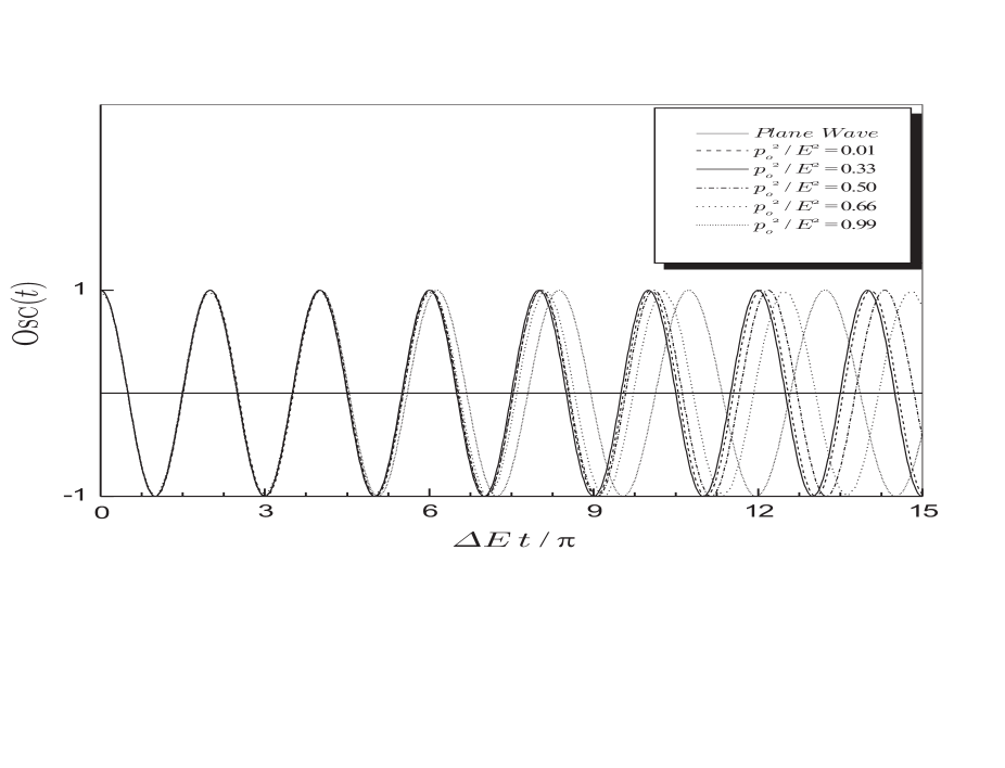
Figure 1: The time-behavior of $\mbox{\sc Osc}(t)$ compared with the standard plane-wave oscillation given by $\cos{[\Delta E\,t]}$ for different propagation regimes. The additional phase $\Theta(t)$ changes the oscillating character after some time of propagation. The minimal deviation occurs for $\frac{p_{\mbox{\tiny$0$}}^{\mbox{\tiny$2$}}}{\bar{E}^{\mbox{\tiny$2$}}}\approx\frac{1}{3}$ which is represented by a solid line superposing the plane-wave case.

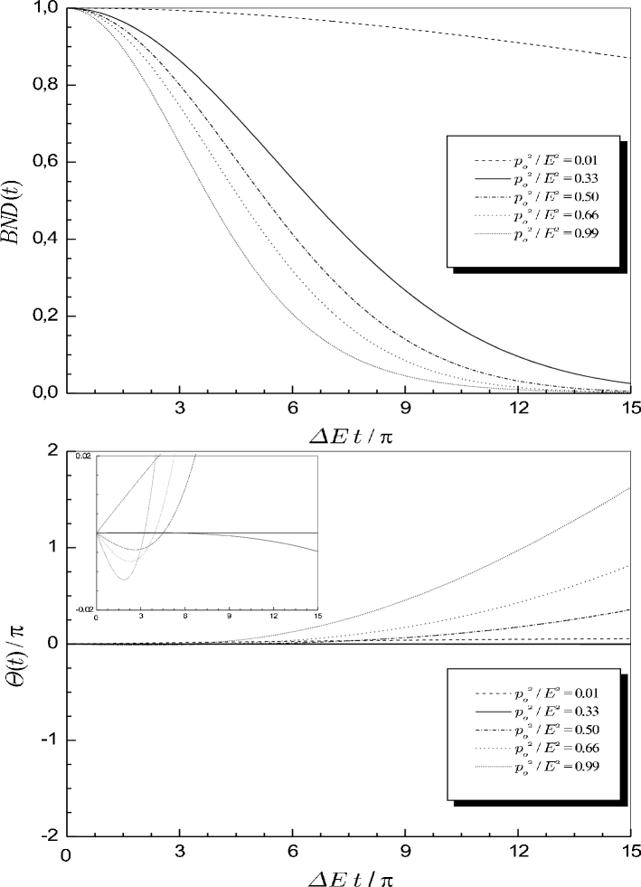
Figure 2: The values assumed by $\Theta(t)$ are effective while the interference term does not vanish. In the upper box we can observe the behavior of $\mbox{\sc Bnd}(t)$ which determines the limit values effectively assumed by $\Theta(t)$ for each propagation regime. For relativistic regimes with $\frac{p_{\mbox{\tiny$0$}}^{\mbox{\tiny$2$}}}{\bar{E}^{\mbox{\tiny$2$}}}>\frac{1}{3}$, the function $\Theta(t)$ rapidly reaches its lower limit as we can observe in the small box above. We have used $a\,\bar{E}=10$.

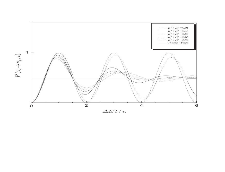
Figure 3: Flavor conversion probability time dependence obtained with the introduction of second-order corrections in the series expansion of the energy for a strictly peaked momentum distribution ($\mathcal{O}(\sigma_{\mbox{\tiny$i$}}^{\mbox{\tiny$3$}})$). By comparing with the PW predictions, depending on the propagation regime, the additional time-dependent phase $\Delta\Phi(t)\equiv\,\Delta E\,t+\Theta(t)$ produces a delay/advance in the local maxima of flavor detection. Phenomenologically, it can introduce small quantifiable deviations to the averaged detected values of neutrino oscillation parameters. Essentially, it depends on the product of the wave-packet width $a$ by the averaged energy $\bar{E}$.

References

[1]\NameK. Zuber
\REVIEWPhys. Rep.3051998295.
[2]\NameW. M. Alberico S. M. Bilenky
\REVIEWProg. Part. Nucl.352004297.
[3]\NameR. D. McKeown P. Vogel
\REVIEWPhys. Rep.3952004315.
[4]\NameM. Beuthe
\REVIEWPhys. Rep.3752003105.
[5]\NameC. Giunti C. W. Kim
\REVIEWPhys. Rev. D581998017301.
[7]\NameA. E. Bernardini S. De Leo
\REVIEWPhys. Rev. D712005076008.
[8]\NameM. Blasone G. Vitiello
\REVIEWAnn. Phys.2441995283.
[9]\NameC. Giunti
\REVIEWJ. High Energy Phys.02112002017.
[10]\NameC. Cohen-Tannoudji, B. Diu F. Laloe
\BookQuantum Mechanics
\Vol1
\PublJohn Wiley & Sons, Paris
\Year1977.
[11]\NameM. Blasone, P. P. Pacheco H. W. Tseung
\REVIEWPhys. Rev. D672003073011.
[12]\NameB. Kayser
\REVIEWPhys. Rev. D241981110.
[13]\NameB. Kayser, F. Gibrat-Debu F. Perrier
\BookThe Physics of Massive Neutrinos
\PublCambridge University Press, Cambridge
\Year1989.
[14]\NameB. Kayser
\REVIEWPhys. Lett. B5922004145, in [PDG Collaboration].
[15]\NameS. De Leo, C. C. Nishi P. Rotelli
\REVIEWInt. J. Mod. Phys. A192004677.
[16]\NameJ. Rich
\REVIEWPhys. Rev. D4819934318.
[17]\NameA. E. Bernardini S. De Leo
\REVIEWEur. Phys. J. C372004471.