Inflation from D3-brane motion in the background of D5-branes

Abstract

We study inflation arising from the motion of a Bogomol’nyi-Prasad-Sommerfield (BPS) D3-brane in the background of a stack of $k$ parallel D5-branes. There are two scalar fields in this set up– (i) the radion field $R$, a real scalar field, and (ii) a complex tachyonic scalar field $\chi$ living on the world volume of the open string stretched between the D3 and D5 branes. We find that inflation is realized by the potential of the radion field, which satisfies observational constraints coming from the Cosmic Microwave Background. After the radion becomes of order the string length scale $l_{s}$, the dynamics is governed by the potential of the complex scalar field. Since this field has a standard kinematic term, reheating can be successfully realized by the mechanism of tachyonic preheating with spontaneous symmetry breaking.

I Introduction

There has been a resurgence of interest in the time-dependent dynamics of extended objects found in the spectrum of string theory, inspired in part by Sen’s construction of a boundary state description of open string tachyon condensation. See, for example, Ref. senrev for review. This description has been supplemented well by an effective theory described by a Dirac Born Infeld (DBI) type action for the tachyon field DBI . More recent work has focused on the dynamics of a probe BPS D-brane in a variety of gravitational backgrounds inspired by the observation that there exists a similarity between the late time dynamics of the probe D-branes and the condensation of the open string tachyon on the world-volume of non-BPS brane in flat space. The latter dynamics is also described by the DBI action kutasov , see also Refs. Sahakyan ; pani ; TW . Both systems describe rolling matter fields which have a vanishing pressure at late times. As a result we can, through an appropriate field transformation, investigate the physics of gravitational backgrounds in terms of non-trivial fields on a brane in flat space using the DBI effective action. This has led to the interesting proposal that the open string tachyon may be geometrical in nature.

Many of the backgrounds that have been probed in this manner have been supergravity (SUGRA) brane solutions of type II string theory. By ensuring that the number of background branes is large we can trust our SUGRA solutions. Moreover we can neglect any back reaction of the probe upon the background geometry. This allows us to use the DBI action to effectively determine the relativistic motion of extended objects in a given background. Quantum corrections can also be calculated in those backgrounds that have an exact Conformal Field Theory (CFT) description Sahakyan . The dynamics of branes in various backgrounds is expected to be relevant for string theory inspired cosmology, just as in the case of open string tachyon matter tachinfl since the field (radion) which parameterizes the distance between the probe brane and the static background branes is a scalar and may be a potential candidate for being the inflaton.

One of the most important theoretical advances in modern cosmology has been the inflationary paradigm, which relies on a scalar field to solve the horizon and flatness problems in the early universe (see Refs. inflation for review). Recent observations from WMAP WMAP , SDSS SDSS and 2dF 2dF impose tight restrictions on the possible mechanisms that can satisfy the paradigm general , and hence provide the interesting possibility for us to test string theoretic inflation models. The observations of Supernova Ia SNIa also suggest that our universe is currently undergoing a period of accelerated expansion, which is attributed to dark energy. It still remains a fundamental problem to describe dark energy in a purely stringy context, although there has been several recent developments darkenergy .

There have been many attempts to embed inflation within string theory. The most popular approach has been to invoke the use of the open string tachyon living on a non-BPS brane as a candidate for the inflaton tachinfl (see Refs. cospep for a number of cosmological aspects of tachyon). Unfortunately it has been shown that this cannot be implemented in a consistent manner, at least in the simplest scenarios KL02 ; Frolov . The other common approach is so-called D-brane inflation in which the separation between branes plays the role of the inflation Dvali ; braneantibrane ; Garcia ; Hirano . In particular this is well accommodated in a form of hybrid inflation where tachyonic open string fluctuations are the fields which end inflation, and another field is chosen to be the inflaton. These open string fluctuations arise in the context of all D-brane cosmological models once the branes are within a string length of one another. A concrete example of this occurs in brane/anti-brane inflation braneantibrane and recently in the context of more phenomenological warped compactifications kklmmt (see also Refs. dbranepapers ). It should be noted that most of the work done in this direction assumes that the dimensionalities of the brane and anti-brane are the same apart from D3/D7 brane inflation models studied in Refs. D3D7 which does not include the open string tachyon dynamics at late times. On the contrary, in our model a probe D3 brane is used to lead to inflation in the presence of static D5 branes (see Refs. TWinf ; PST for related works) and the open string tachyon dynamics naturally comes in. In any event there has been very little work done on trying to understand the relationship between inflation and the current dark energy phase which we observe.

A potential solution for both inflation and dark energy, in this context, can be obtained as a mixture of these two scenarios. We require a mechanism which drives inflation independently of the open string tachyon, but then falls into the tachyonic state at late times. This can be achieved by considering the motion of a D3-brane in a type IIB background. By switching to our holographic picture of a non-trivial field on a non-BPS brane kutasov we will find that the radion field naturally exits from inflation once it reaches a critical velocity. If this occurs at a distance larger than the string length, we can then use the open string tachyon, which sets in at a distance equal to or less than the string length, to explain the dark energy content of the universe.

In this paper we aim to explore the motion of a probe D3-brane in the background of $k$ coincident, static D5-branes. For simplicity we will neglect any closed string radiation which would be emitted from the probe brane as it travels down the throat generated by the background branes. We will also neglect any gauge fields which may exist on the D3-brane world-volume. Note that this is S-dual to the solution considered in Ref. kutasov . In order to make contact with four dimensional physics we must consider the dual picture of a non-trivial field on a non-BPS brane in flat space, where we also toroidally compactify the remaining six dimensions. We will assume that there is some mechanism which freezes the various moduli of the compactification manifold so that they do not appear in the effective action. The resulting theory should represent the leading order contribution which would arise from compactifying the full type IIB background. At distances large compared to the string scale, the DBI description is known to be valid, however once the probe brane approaches small distances (order of string length scale) we must switch to the open string analysis. Open strings will stretch from the D3-brane to the D5-branes, and their fluctuation spectrum contains a tachyonic mode. Thus when the separation is order of the string length, the DBI description will no longer be valid and we must resort to a purely open string analysis. We expect that inflation will occur in the large field (radion) regime and it ends before the separation comes closer to string length and that as the branes get closer, the open string tachyon reheats the universe.

This paper is organized as follows. In the next section we describe the dynamics of a single probe D3-brane in the presence of a large number of static background D5-branes. Because of the dimensionalities of the branes we expect to find an open string tachyonic mode once we begin to probe distances approaching the string length branonium . In section III, we present the inflation dynamics and observational constraints on the various parameters of our model. In section IV, we discuss the role of the open string tachyon after the inflationary phase and the possibility of reheating in our model and a brief discussion on dark energy. In the last section, we present some of our conclusions and future outlook.

II D3-brane dynamics in D5-brane background

In this section we analyze the motion of a probe BPS D3-brane in the background generated by a stack of coincident and static BPS D5-branes. The background fields, namely the metric, the dilaton $(\phi)$ and the Ramond-Ramond (RR) field $(C)$ for a system of $k$ coincident D5-branes are given by Callan ; kutasov

$$g_{\alpha\beta} = F^{-1/2}\eta_{\alpha\beta},~{}~{}g_{mn}=F^{1/2}\delta_{mn},$$

$$e^{2\phi} = F^{-1}=~{}C_{0...5},~{}~{}F=1+\frac{kg_{s}l_{s}^{2}}{r^{2}}\,,$$ (1)

where $\alpha,\beta=0,..,5;~{}m,n=6,...,9$ denote the indices for the world volume and the transverse directions respectively and $F$ is the harmonic function describing the position of the $k$ D5-branes and satisfying the Green function equation in the transverse four dimensional space. Here $g_{s}$ and $l_{s}=\sqrt{\alpha^{\prime}}$ are the string coupling and the string length, respectively. $r$ is the radial coordinate away from the D5-branes in the transverse direction. The solution parameterizes a throat-like geometry which becomes weakly coupled as we approach the source branes.

The motion of the D3-brane in the above background can be studied in terms of an effective DBI action, on its world volume, given by kutasov

$${\mathcal{S}_{0}}=-\tau_{3}\int{\rm d}^{4}xF^{-1/2}\sqrt{1+F\partial_{\alpha}R\partial^{\alpha}R}\,,$$ (2)

where $\tau_{3}$ is the tension of the 3-brane. Here the motion of the probe brane is restricted to be purely radial fluctuation, denoted by the mode $R$, along the common four dimensional transverse space. This action is the same as that considered in Ref. kutasov . The background considered here is the S-dual to the background considered there and we have not kept the contribution of the RR fields in the action. The form of the above action resembles the DBI action of the tachyon field in the open string ending on a non-BPS D3-brane in a flat background. This is given by

$${\mathcal{S}_{1}}=-\int{\rm d}^{4}xV(T)\sqrt{1+\partial_{\alpha}T\partial^{\alpha}T}\,.$$ (3)

Comparison of the above two actions defines a “tachyon” field $T$ by the relation:

$$\frac{{\rm d}T}{{\rm d}R}=\sqrt{F(R)}=\sqrt{1+L^{2}/R^{2}}\,,$$ (4)

where

$$L\equiv\sqrt{kg_{s}}l_{s}\,.$$ (5)

In terms of this field the “tachyon potential” in Eq. (3) is given by

$$V=\frac{\tau_{3}}{\sqrt{F(R)}}=\frac{\tau_{3}}{\sqrt{1+L^{2}/R^{2}}}\,.$$ (6)

One can solve Eq. (4) for the $T(R)$ and find it to be a monotonically increasing function kutasov :

$$T(R)=\sqrt{L^{2}+R^{2}}+{1\over 2}L\ln{{\sqrt{L^{2}+R^{2}}-L}\over{{\sqrt{L^{2}+R^{2}}+L}}}.$$ (7)

This function is non-invertible but can be simplified by exploring limits of the field space solution. As $R\rightarrow 0$ we have $T(R)\rightarrow-\infty$ with dependence

$$T(R\rightarrow 0)\simeq L\ln{{R\over L}}\,.$$ (8)

As $R\rightarrow\infty$ we have $T(R)\rightarrow\infty$ with

$$T(R\rightarrow\infty)\simeq R\,.$$ (9)

The effective potential in these two asymptotic regions is given by:

$$\frac{V(T)}{\tau_{3}} \simeq \exp\left(\frac{T}{L}\right)\qquad{\rm for}\quad T\rightarrow-\infty\,,$$ (10)

$$\simeq 1-\frac{1}{2}\frac{L^{2}}{T^{2}}\qquad{\rm for}\quad T\rightarrow\infty\,.$$ (11)

Figure 1: The potential of the field $T$. The value $T_{*}=[\sqrt{2}+{\rm ln}\,(\sqrt{2}-1)]L$ is determined by the condition $R=L$. The potential of the region (i) is approximately given by $V(T)=\tau_{3}\exp(T/L)$, whereas $V(T)=\tau_{3}(1-L^{2}/2T^{2})$ in the region (ii).

Thus in the limit $T\rightarrow-\infty$, corresponding to $R\rightarrow 0$, one observes that the potential goes to zero exponentially (see Fig. 1). This is consistent with the late time behavior for the open string tachyon potential in the rolling tachyon solutions and leads to exponential decrease of the pressure at late times sen2 . The “tachyon field” has a geometric meaning signifying the distance between the probe brane and the D5-branes. At large distances, the DBI action interpolates smoothly between standard gravitational attraction among the probe and the background branes and a “radion matter” phase when the probe brane is close to the five branes. The transition between the two behaviors occurs at $R\sim L$.

It is important to note that when the probe brane is within the distance $R\sim l_{s}$, the above description in terms of the closed string background is inappropriate and the system should be studied using upon strings stretched between the probe brane and the five branes. To be more precise, when the probe brane comes to within a distance between $l_{s}$ from the D5-branes, a tachyon appears in the open string spectrum and in principle the dynamics of the system will be governed by its condensation from that point on.

Thus the full dynamics can be divided into two regimes. When the distance $R$ between the D3-brane and the D5-branes is much smaller than $L$ but larger than $l_{s}$, we can describe the dynamics of the radial mode $R(x^{\mu})$ by the tachyon matter Lagrangian (3) with an exponentially decaying potential given by (10) (note that $T$ is going toward $-\infty$). On the contrary, when $R$ is of the order of $l_{s}$, the dynamics would be be governed by the conventional Lagrangian describing the complex tachyonic scalar field $\chi$ present in the open string stretched between the D3-brane and the $k$ D5-branes. The potential for such open string tachyon field has already been calculated Gava . Thus the dynamics of $\chi$ is described by the action:

$${\mathcal{S}_{2}}=\int{\rm d}^{4}x[-\partial_{\alpha}\chi\partial^{\alpha}\chi^{*}-U(\chi,\chi^{*})]\,,$$ (12)

where the potential, up to quartic order, is given by:

$$U(\chi,\chi^{*})=\frac{1}{4\pi^{4}l_{s}^{4}g_{s}k}\left[\pi(k+1)(\chi\chi^{*})^{2}-v\chi\chi^{*}\right]\,.$$ (13)

Note that $\chi$ and $v$ are dimensionless quantities. Here $v$ is a small parameter ($v\ll k$) corresponding to the volume of a two torus. This arises as we are toroidally compactifying the directions transverse to the D3-brane, but parallel to the D5-branes, in order to describe the dynamics of the open string tachyon. When we map the theory to our purely $3+1$ dimensional subspace, we will neglect any string winding modes arising from this torus. Furthermore it can be seen that our fully compactified theory is actually not $T^{6}$ but the product space $T^{4}\times T^{2}$ but for simplicity we shall assume that the relevant radii are approximately equal.

Let us briefly recapitulate and consider the bulk dynamics in more detail. At distances larger than the string length we know that the DBI action provides a good description of the low energy physics for a probe brane in the background geometry. As mentioned in the introduction, the D3-brane is much lighter than the coincident D5-branes and so we can neglect the back reaction upon the geometry. Furthermore the SUGRA solution indicates that the string coupling tends to be zero as we probe smaller distances, providing a suitable background for perturbative string theory and implying that we can trust our description down to small distances without requiring a bound on the energy kutasov .

Because of the dimensionalities of the branes in the problem there is no coupling of the D3-brane to the bulk RR six form. This is because the only possible Wess-Zumino interaction between the probe brane and the background can be through the self dual field strength $\tilde{f}={\rm d}\tilde{C}_{(4)}$. However this field strength must be the Hodge dual of the background field strength - which is given here by $f={\rm d}C_{(6)}$ for D5-branes - clearly this inconsistency implies that the coupling term will vanish. For a more detailed explanation of the more general case we refer the reader to the paper branonium , however the basic result for our purpose is that there is only a non-zero interaction term when either the dimensionality of probe and background branes are the same, or they add up to six. The probe brane however does possess its own RR charge which ought to be radiated as the brane rolls in the background, but for simplicity we will neglect this in our analysis.

The energy-momentum tensor density of the probe brane in the background can be calculated as

$$T_{ab} = \frac{\tau_{3}}{\sqrt{F}}\Biggl{(}\frac{F\partial_{a}R\partial_{b}R}{\sqrt{1+F\eta^{cd}\partial_{c}R\partial_{d}R}}$$ (14)

$$-\eta_{ab}\sqrt{1+F\eta^{cd}\partial_{c}R\partial_{d}R}\Biggr{)},$$

where the roman indices are directions on the world-volume. As we are only interested in homogenous scalar fields in this paper, we find that this expression reduces to

$$T_{00} = \frac{\tau_{3}}{\sqrt{F}\sqrt{1-F\dot{R}^{2}}}\,,$$

$$T_{ij} = -\frac{\tau_{3}\delta_{ij}\sqrt{1-F\dot{R}^{2}}}{\sqrt{F}},$$ (15)

where $i,j$ are now the spatial directions on the D3-brane.

Using the energy conservation we can obtain the equation of motion for the probe brane in our background and estimate its velocity. By imposing the initial condition that the velocity is zero at the point $R=R_{0}$ we find that the expression for the velocity reduces to

$$\dot{R}^{2}=\frac{R^{2}L^{2}}{(R^{2}+L^{2})^{2}}\left(1-\frac{R^{2}}{R_{0}^{2}}\right),$$ (16)

which is obviously valid for $R\leq R_{0}$ and in fact as expected it vanishes identically at $R=R_{0}$. We typically would expect $R_{0}$ to be extremely large. Note that in the two asymptotic regions of small and large $R$ the velocity is tending to zero. This is understood because the throat geometry acts as a gravitational red-shift, giving rise to D-cceleration phenomenon tong . It should be emphasised that the asymptotic limit $R\to 0$ is unphysical because the DBI is not valid once we reach energies of the order of string mass $M_{s}$, and so it is not strictly correct to say that the velocity goes to zero in the small $R$ approximation. However note that when $R\rightarrow l_{s}$ we have $\dot{R}^{2}\sim l_{s}^{2}/L^{2}=1/kg_{s}$ which is also negligibly small for large $k$. From our perspective this implies that the kinetic energy of the scalar field become sub-dominant at small distances. It is essentially frozen out and the dynamics of the open string tachyonic modes come to dominate. Once the probe brane reaches distances comparable with the string length our closed string description is no longer valid. Instead we must switch over to an open string description of the tachyonic modes $\chi$ described by the action (12).

It is worth pointing out that our discussion so far seems to suggest that the radionic mode and the open string tachyonic mode which are being described by two different action functionals have nothing in common and can be described independent of each other. However, it is not so. First the number of background branes have to be same. Secondly, unlike the open string tachyon on the world volume of a non-BPS brane or a brane/anti-brane pair, the dynamics of the tachyon on the open string connecting a BPS D$p$-brane and a BPS D$(p+2)$-brane is not described by a DBI type action. If this would have been the case, the above two fields could have been combined together with keeping in mind about their region of validity.

However, even in the present context we can combine the two actions by introducing an interaction term like $\lambda T^{2}\chi^{2}$ where the coupling $\lambda$ will be zero for values of the field $T$ corresponding to $R$ greater than $l_{s}$. Provided that inflation ends for $R>l_{s}$, this term does not affect the dynamics of inflation and for simplicity we have ignored it in the action functional. However, such a term may play an important role in a possible reheating phase. We can now proceed with our analysis of inflation using the full form of the harmonic function - which specifies the scalar field potential in terms of the geometrical tachyon field rather than the radion field.

III Inflation and observational constraints from CMB

In this section we shall discuss the dynamics of inflation and observational constraints on the model (6) from CMB. Introducing a dimensionless quantity $x\equiv R/L$, the full potential (6) of the field $T$ is written as

$$V=\frac{x}{\sqrt{x^{2}+1}}\tau_{3}\,,$$ (17)

where $\tilde{T}\equiv T/L$ is related to $x$ via

$$\frac{{\rm d}\tilde{T}}{{\rm d}x}=\frac{\sqrt{x^{2}+1}}{x}=\frac{1}{\tilde{V}}\,,$$ (18)

where $\tilde{V}\equiv V/\tau_{3}$. We require that $R$ is larger than $l_{s}$, which translates into the condition $x>1/\sqrt{kg_{s}}$.

In a flat Friedmann-Robertson-Walker background with a scale factor $a$ the field equations are cospep

$$H^{2}=\frac{1}{3M_{p}^{2}}\frac{V(T)}{\sqrt{1-\dot{T}^{2}}}\,,$$ (19)

$$\frac{\ddot{T}}{1-\dot{T}^{2}}+3H\dot{T}+\frac{V_{T}}{V}=0\,,$$ (20)

where $H\equiv\dot{a}/a$ is the Hubble rate, $V_{T}\equiv{\rm d}V/{\rm d}T$, and $M_{p}=1/\sqrt{8\pi G}$ is the 4-dimensional reduced Planck mass ($G$ is the gravitational constant).

Combining Eq. (19) and (20) gives the relation $\dot{H}/H^{2}=-3\dot{T}^{2}/2$. Then the slow-roll parameter is given by

$$\epsilon \equiv -\frac{\dot{H}}{H^{2}}=\frac{3}{2}\dot{T}^{2}\simeq\frac{M_{p}^{2}}{2}\frac{V_{T}^{2}}{V^{3}}$$ (21)

$$= \frac{1}{2s}\frac{\tilde{V}_{x}^{2}}{\tilde{V}}=\frac{1}{2s}\frac{1}{x(x^{2}+1)^{5/2}}\,,$$

where $s$ is defined by

$$s\equiv\frac{L^{2}\tau_{3}}{M_{p}^{2}}\,.$$ (22)

In deriving the slow-roll parameter we used the slow-roll approximation $\dot{T}^{2}\ll 1$ and $|\ddot{T}|\ll 3H|\dot{T}|$ in Eqs. (19) and (20). Equation (21) shows that $\epsilon$ is a decreasing function in terms of $x$. Hence $\epsilon$ increases as the field evolves from the large $R$ region to the small $R$ region, marking the end of inflation at $\epsilon=1$.

The number of $e$-foldings from the end of inflation is

$$N \equiv \int_{t}^{t_{f}}H{\rm d}t\simeq\int^{T}_{T_{f}}\frac{V^{2}}{M_{p}^{2}V_{T}}{\rm d}T$$ (23)

$$= s\int^{x}_{x_{f}}(x^{2}+1)^{3/2}{\rm d}x\,.$$

This is integrated to give

$$N=s[f(x)-f(x_{f})]\,,$$ (24)

where

$$f(x) = \frac{1}{4}x(x^{2}+1)^{3/2}+\frac{3}{8}x\sqrt{x^{2}+1}$$ (25)

$$+\frac{3}{8}{\rm ln}\left|x+\sqrt{x^{2}+1}\right|\,.$$

The function $f(x)$ grows monotonically from $f(0)=0$ to $f(\infty)=\infty$ with the increase of $x$. In principle we can obtain a sufficient amount of inflation to satisfy $N>70$ if either $s$ or $x$ is large.

In order to confront with observations we need to consider the spectra of scalar and tensor perturbations generated in our model. The power spectrum of scalar metric perturbations is given by Hwang ; SV04 ; GST

$${\cal P}_{\rm S} = \frac{1}{12\pi^{2}M_{p}^{6}}\left(\frac{V^{2}}{V_{T}}\right)^{2}=\frac{\tau_{3}^{2}L^{2}}{12\pi^{2}M_{p}^{6}}\left(\frac{\tilde{V}}{\tilde{V}_{x}}\right)^{2}$$ (26)

$$= \frac{s^{2}}{12\pi^{2}kg_{s}(l_{s}M_{p})^{2}}x^{2}(x^{2}+1)^{2}\,.$$

The COBE normalization corresponds to ${\cal P}_{\rm S}=2\times 10^{-9}$ around $N=60$ inflation , which gives

$$kg_{s}(l_{s}M_{p})^{2}=\frac{10^{9}}{24\pi^{2}}s^{2}x_{60}^{2}(x_{60}^{2}+1)^{2}\,.$$ (27)

The spectral index of curvature perturbations is given by Hwang ; SV04 ; GST

$$n_{\rm S}-1 = -4\frac{M_{p}^{2}V_{T}^{2}}{V^{3}}+2\frac{M_{p}^{2}V_{TT}}{V^{2}}$$ (28)

$$= -\frac{2}{s}\frac{1+3x^{2}}{x(1+x^{2})^{5/2}}\,,$$

whereas the ratio of tensor to scalar perturbations is

$$r=8\frac{V_{T}^{2}M_{p}^{2}}{V^{3}}=\frac{8}{s}\frac{1}{x(x^{2}+1)^{5/2}}\,.$$ (29)

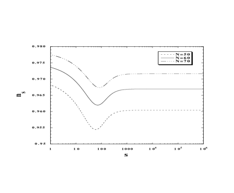
Figure 2: The spectral index $n_{\rm S}$ of scalar metric perturbations as a function of $s$ with three different number of $e$-foldings ($N=50,60,70$). This figure corresponds to the case in which inflation ends in the region $x_{f}\ll 1$.

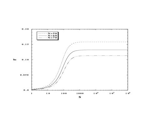
Figure 3: The tensor-to-scalar ratio $r$ as a function of $s$ with three different number of $e$-foldings ($N=50,60,70$).

We shall study the case in which the end of inflation corresponds to the region with an exponential potential, i.e., $x_{f}\ll 1$. When $s=1$, Eq. (21) shows that inflation ends around $x_{f}\sim 0.5$. Hence the approximation, $x_{f}\ll 1$, is valid when $s$ is larger than of order unity. In this case one has $x_{f}\simeq 1/2s$ from Eq. (21). Since $f(x)\simeq x$ for $x\ll 1$, we find

$$f(x)=(N+1/2)/s\,.$$ (30)

In the regime of an exponential potential ($x\ll 1$) we have $sx\simeq N+1/2$. In this case Eqs. (28) and (29) give

$$n_{\rm S}-1 = -\frac{4}{2N+1}\,,$$ (31)

$$r = \frac{16}{2N+1}\,.$$ (32)

Hence $n_{\rm S}$ and $r$ are dependent on the number of $e$-foldings only. From Eqs. (31) and (32) we find that $n_{\rm S}=0.9669$ and $r=0.1322$ for $N=60$. It was shown in Ref. GST that this case is well inside the $1\sigma$ contour bound coming from the observational constraints of WMAP, SDSS and 2dF (see also Ref. SV04 ).

Figure 4: The quantity $kg_{s}(l_{s}M_{p})^{2}$ as a function of $s$. This is derived by the COBE normalization at $N=60$.

Of course there is a situation in which cosmologically relevant scales ($55\lesssim N\lesssim 65$) correspond to the region $x\gtrsim 1$. In Figs. 2 and 3 we plot $n_{\rm S}$ and $r$ as a function of $s$ for three different values of $N$. For large $s(\gg 1)$, we find that the quantity $x$ is much smaller than unity from the relation (30). Hence $n_{\rm S}$ and $r$ are given by the formula (31) and (32). For smaller $s$ the quantity $x$ becomes larger than of order unity, which means that the results (31) and (32) can no longer be used. In Fig. 2 we find that the spectral index has a minimum around $s=70$ for $N=60$. This roughly corresponds to the region $x=R/L\sim 1$. As we see from Fig. 1 the potential becomes flatter for $x\gtrsim 1$. This leads to the increase of the spectral index toward $n_{\rm S}=1$ with the decrease of $s$. Recent observations show that $n_{\rm S}=0.98\pm 0.02$ at the 95% confidence level Seljak (see also Refs. inobser ). As we find in Fig. 2 this condition is satisfied for $N\gtrsim 60$.

The tensor-to-scalar ratio is given by Eq. (32) for $s\gg 1$. For a fixed value of $N$ this ratio gets smaller with the decrease of $s$. This is understandable, since the potential becomes flatter as we enter the region $x\gtrsim 1$. The tensor-to-scalar ratio is constrained to be $r<0.36$ at the 95% confidence level from recent observations Seljak . Hence our model satisfies this observational constraint.

When $x_{60}\ll 1$ the condition of the COBE normalization (27) gives

$$kg_{s}(l_{s}M_{p})^{2}\simeq\frac{10^{9}}{24\pi^{2}}(60+1/2)^{2}\simeq 1.55\times 10^{10}\,,$$ (33)

which is independent of $s$. As we see from Fig. 4 the quantity $kg_{s}(l_{s}M_{p})^{2}$ departs from the value (33) for smaller $s$. However $kg_{s}(l_{s}M_{p})^{2}$ is of order $10^{10}$ for $s\gtrsim 1$. It is interesting to note that the COBE normalization uniquely fixes the value of the potential at the end of inflation if it happens in the regime of an exponential potential independently of the fact where inflation had commenced. In fact using Eq. (17) gives

$$V_{\rm end}\simeq x_{f}\tau_{3}=\frac{1}{2kg_{s}(l_{s}M_{p})^{2}}M_{p}^{4}\simeq 3.2\times 10^{-11}M_{p}^{4}\,.$$ (34)

This sets the energy scale to be $V^{1/4}_{\rm end}\simeq 2.3\times 10^{-3}M_{p}$.

The above discussion corresponds to the case in which inflation ends in the region $x_{f}\ll 1$. In order to understand the behavior of another asymptotical region, let us consider a situation when inflation ends for $x_{f}\gg 1$. In this case the end of inflation is characterized by $x_{f}^{6}\simeq 1/(2s)$. Since $x_{f}\gg 1$, we are considering a parameter range $s\ll 1$. When $x\gg 1$ the function $f(x)$ behaves as $f(x)\simeq x^{4}/4$, which gives the relation $x^{4}\simeq 4N/s$. Hence we obtain

$$n_{\rm S}-1 = -\frac{3}{2N}\,,$$ (35)

$$r = \frac{\sqrt{s}}{N^{3/2}}\,,$$ (36)

$$kg_{s}(l_{s}M_{p})^{2} = \frac{10^{9}\sqrt{2}N^{3/2}}{6\pi^{2}}\sqrt{s}\,.$$ (37)

While $n_{\rm S}$ is independent of $s$, both $r$ and $kg_{s}(l_{s}M_{p})^{2}$ are dependent on $s$ and $N$. For example one has $n_{\rm S}=0.975$, $r=0.003\sqrt{s}$ and $kg_{s}(l_{s}M_{p})^{2}=1.11\times 10^{10}\sqrt{s}$ for $N=60$. From Fig. 2 we find that $n_{\rm S}$ increases with the decrease of $s$ in the region $1\lesssim s\lesssim 50$ for a fixed $N$. This tendency persists for $s\lesssim 1$ and $n_{\rm S}$ approaches a constant value given by Eq. (35) as $s$ decreases. We note that the spectral index $n_{\rm S}$ satisfies the observational constraint coming from recent observations. The tensor-to-scalar ratio is strongly suppressed in the region $s<1$, which also satisfies the observational constraint. The quantity $kg_{s}(l_{s}M_{p})^{2}$ gets smaller with the decrease of $s$.

We can estimate the the potential energy at the end of inflation in the regime described by $x_{f}\gg 1$, as

$$V_{\rm end} \simeq \tau_{3}\,,$$ (38)

$$\tau_{3} = \frac{s}{kg_{s}(l_{s}M_{p})^{2}}M_{p}^{4}\simeq 9.0\times 10^{-11}\sqrt{s}M_{p}^{4}\,.$$ (39)

In this case $V_{\rm end}$ depends on the value of $s$. The order of the energy scale does not differ from (34) provided that $s$ is not too much smaller than unity.

In summary we find that $n_{\rm S}$ and $r$ in our model satisfy observational constraints of CMB for any values of $s$, which means that we do not obtain the constraint on $s$. This is different from the geometrical tachyon inflation with potential $V=V_{0}\cos(T/\sqrt{kl_{s}^{2}})$ in which the spectral index $n_{\rm S}$ provides constrains on model parameters PST . The only constraint in our model is the COBE normalization. If we demand that the value of $R$ at the end of inflation is larger than $l_{s}$, this gives

$$k<16\pi^{6}g_{s}\left(\frac{M_{p}}{M_{s}}\right)^{4}\,,$$ (40)

where we used $\tau_{3}=M_{s}^{4}/(2\pi)^{3}g_{s}$.

Combining this relation with the condition of the COBE normalization: $kg_{s}(l_{s}M_{p})^{2}\simeq 10^{10}$ for $s\gtrsim 1$, we find

$$g_{s}>\frac{10^{5}}{4\pi^{3}}\left(\frac{M_{s}}{M_{p}}\right)^{3}\,.$$ (41)

Since we require the condition $g_{s}\ll 1$ for the validity of the theory, this gives the constraint

$$M_{s}/M_{p}\ll 0.1\,.$$ (42)

After the field reaches the point $R=l_{s}$, we assume that the field $T$ is frozen at this point, which is a reasonable assumption given what we understand from the bulk description of the dynamics. This gives us a positive cosmological constant in the system.

IV After the end of inflation

The first phase driven by the field $T$ is triggered by the second phase driven by the field $\chi$. Introducing new variables $\chi=\chi_{1}+i\chi_{2}$, $X^{2}=\chi_{1}^{2}+\chi_{2}^{2}$, $\tilde{X}=M_{p}X$ and $\tilde{v}=M_{p}^{2}v$, the potential (13) of the field $X$ reduces to

$$U(\tilde{X})=\frac{1}{4\pi^{4}(l_{s}M_{p})^{4}g_{s}k}\left[\pi(k+1)\tilde{X}^{4}-\tilde{v}\tilde{X}^{2}\right]\,.$$ (43)

This potential has two local minima at $\tilde{X}_{c}=\pm\sqrt{\tilde{v}/(2\pi(k+1))}$ with negative energy

$$U(\tilde{X}_{c})=-\frac{\tilde{v}^{2}}{16\pi^{5}k(k+1)(l_{s}M_{p})^{4}g_{s}}\,.$$ (44)

One can cancel (or nearly cancel) this term by taking into account the energy of the field $T$ at $R=l_{s}$. Since this is given by $V(R=l_{s})=\tau_{3}/\sqrt{kg_{s}}$, the condition $V(R=l_{s})+U(\tilde{X}_{c})=0$ leads to

$$\tilde{v}^{2}=16\pi^{5}(k+1)\tau_{3}(l_{s}M_{p})^{4}\sqrt{kg_{s}}\,.$$ (45)

Using the relation $\tau_{3}=M_{s}^{4}/(2\pi)^{3}g_{s}$, this can be written as

$${\tilde{v}}^{2}=\frac{2\pi^{2}\sqrt{k}(k+1)}{\sqrt{g_{s}}}\,.$$ (46)

Then the total potential of our system is

$$W=A\left(\tilde{X}^{2}-\tilde{X}_{c}^{2}\right)^{2}\,,$$ (47)

where

$$A\equiv\frac{k+1}{4\pi^{3}(l_{s}M_{p})^{4}g_{s}k}\,.$$ (48)

The mass of the potential at $\tilde{X}=0$ is given by

$$m^{2}\equiv\frac{{\rm d}^{2}W}{{\rm d}\tilde{X}^{2}}(\tilde{X}=0)=-4A\tilde{X}_{c}^{2}\,.$$ (49)

Meanwhile the square of the Hubble constant at $\tilde{X}=0$ is

$$H_{0}^{2}=\frac{A\tilde{v}^{2}}{12\pi^{2}(k+1)^{2}M_{p}^{2}}\,.$$ (50)

Then we obtain the following ratio

$$\frac{|m^{2}|}{H_{0}^{2}}=\frac{24\pi(k+1)}{v}=\frac{12\sqrt{2}(k+1)^{1/2}}{k^{1/4}}g_{s}^{1/4}\,,$$ (51)

where we used Eq. (46) in the second equality.

As we showed in the previous section, the COBE normalization gives $kg_{s}(l_{s}M_{p})^{2}\simeq 10^{10}$ for $s\gtrsim 1$. Then the ratio (51) can be estimated as

$$\frac{|m^{2}|}{H_{0}^{2}} \simeq 5\times 10^{3}\left(\frac{k+1}{k}\right)^{1/2}\left(\frac{M_{s}}{M_{p}}\right)^{1/2}$$ (52)

$$\simeq 5\times 10^{3}\left(\frac{M_{s}}{M_{p}}\right)^{1/2}\,.$$

Then we have $|m^{2}|>H_{0}^{2}$ for

$$M_{s}/M_{p}>4\times 10^{-8}\,.$$ (53)

This means that the second stage of inflation does not occur for the field $\chi$ provided that the string mass scale $M_{s}$ satisfies the condition (53). When $4\times 10^{-8}<M_{s}/M_{p}\ll 10^{-1}$, inflation ends before the field $T$ reaches the point $R=l_{s}$, which is triggered by a fast roll of the field $\chi$. This situation is similar to the original hybrid inflation model Linde94 .

When $M_{s}/M_{p}<4\times 10^{-8}$, double inflation occurs even after the end of the first stage of inflation. In this case the CMB constraints discussed in the previous section need to be modified. However the second stage of inflation is absent for the natural string mass scale which is not too much smaller than the Planck scale.

We note that the vacuum expectation value of the field $\tilde{X}$ is given by

$${\tilde{X}}_{c}=2\sqrt{3}\frac{H_{0}}{|m|}M_{p}\,.$$ (54)

When $|m|\gtrsim H_{0}$ we find that $\tilde{X}_{c}$ is less than of order the Planck mass. When double inflation occurs ($|m|\lesssim H_{0}$), the amplitude of symmetry breaking takes a super-Planckian value $\tilde{X}_{c}\gtrsim M_{p}$. In this sense the latter case does not look natural compared to the case in which the second stage of inflation does not occur.

Since the field $\chi$ has a standard kinematic term, reheating proceeds as in the case of potentials with spontaneous symmetry breaking. This is in contrast to a tachyon field governed by the DBI action in which the energy density of the tachyon overdominates the universe soon after the end of inflation. Thus the problem of reheating present in DBI tachyon models KL02 ; Frolov is absent in our model. Since the potential of the field $X$ has a negative mass given by Eq. (49), this leads to the exponential growth of quantum fluctuations of $X$ with momenta $k<|m|$, i.e., $\delta X_{k}\propto\exp(\sqrt{|m^{2}|-k^{2}}\,t)$ Boy . This negative instability is so strong that one can not trust perturbation theory including the Hartree and $1/N$ approximations. We require lattice simulations in order to take into account rescattering of created particles and the production of topological defects Felder .

It was shown in Refs. Felder that symmetry breaking ends after one oscillation of the field distribution as the field evolves toward the potential minimum. This refects the fact that gradient energies of all momentum modes do not return back to the original state at $X=0$ because of a very complicated field distribution after the violent growth of quantum fluctuations.

Finally we should mention that de-Sitter vacua can be obtained provided that the potential energy $V(R=l_{s})$ does not exactly cancel the negative energy $U(\tilde{X}_{c})$. In order to match with the current energy scale of dark energy, we require an extreme fine tuning $V(R=l_{s})+U(\tilde{X}_{c})\simeq 10^{-123}M_{p}^{4}$. However this kind of fine tuning is a generic problem of dark energy.

V Conclusions

In this paper we studied the motion of a BPS D3-brane in the presence of a stack of $k$ parallel D5-branes in type II string theory. Inflation is realized by the potential energy of a radion field $R$ which characterizes the distance of D3 and D5 branes. This potential is not in general written explicitly, but is approximately given by (10) for $R\ll\sqrt{kg_{s}}l_{s}$ and (11) for $R\gg\sqrt{kg_{s}}l_{s}$. We evaluated the spectral index of scalar metric perturbations and the tensor-to-scalar ratio together with the number of $e$-foldings under the condition that inflation ends in the region $R\ll\sqrt{kg_{s}}l_{s}$. This model satisfies observational constraints coming from CMB, SDSS and 2dF independently of the value of $s$ defined by Eq. (22). We also note that this result does not change even when inflation ends in the region $R\gg\sqrt{kg_{s}}l_{s}$.

The only strong constraint coming from CMB is the COBE normalization, i.e., $kg_{s}(l_{s}M_{p})^{2}\simeq 10^{10}$ for $s\gtrsim 1$. If we demand that the inflationary period is over before the radion reaches the point $R=l_{s}$, this gives the constraint on the number of D5-branes; see Eq. (40). Combining this with the condition of the COBE normalization, the string mass scale is constrained to be $M_{s}/M_{p}\ll 0.1$ for the validity of the weak-coupling approximation ($g_{s}\ll 1$).

When the radion field enters the region $R\lesssim l_{s}$, the description of closed string background is no longer valid. Instead the dynamics should be studied using a complex scalar field $\chi$ living on the world volume of open strings stretched between the probe D3-brane and the D5-branes. We assumed that the radion field is frozen in the region $R\lesssim l_{s}$, which gives rise to a positive cosmological constant. The potential of the field $\chi$ is given by Eq. (13), which has a negative energy at the potential minimum. If this energy is cancelled by the positive cosmological constant, we obtain the double-well potential given by Eq. (47).

We found that the absolute value of the mass of this double-well potential at $\chi=0$ is larger than the Hubble parameter provided that $M_{s}/M_{p}>4\times 10^{-8}$. Hence in this case the second stage of inflation does not occur and the evolution of the field $\chi$ is described by a fast roll. Since the action of the complex field has a standard kinematic term, the problem of reheating present in DBI tachyon models is absent in our scenario. Reheating in our model is described by tachyonic preheating in which quantum fluctuations grow exponentially by a negative instability. The symmetry breaking would end after one oscillation of the field distribution as the field evolves toward the potential minimum.

It is also possible to explain the origin of dark energy if a positive cosmological constant does not exactly cancel the negative potential energy of the field $\chi$. Although this requires a fine tuning, it is intriguing that our model provides a number of promising ways to provide viable cosmological evolution.

One of the potential problems with our model is that the compactification is not necessarily realistic. Although we can encode the physics of the gravity background as a non-trivial scalar field on a flat brane, we are treating this latter object as being fundamental. Thus by compactifying this on a $T^{6}$ we will be missing higher order terms coming from the full compactification of the D5-solution. These terms may play a more important role in the cosmological theory on the D3-brane. It may be useful to compare the results obtained in this paper with a full string compactification by smearing the SUGRA harmonic function on a $T^{4}$ and compactifying the remaining directions on the two-cycles of a torus. The resultant analysis is complicated since the DBI may not be valid, however this is beyond the scope of the current endeavor.

References

- (1) A. Sen, arXiv:hep-th/0410103.
- (2) A. Sen, JHEP 9910, 008 (1999); M. R. Garousi, Nucl. Phys. B584, 284 (2000); Nucl. Phys. B 647, 117 (2002); JHEP 0305, 058 (2003); E. A. Bergshoeff, M. de Roo, T. C. de Wit, E. Eyras, S. Panda, JHEP 0005, 009 (2000); J. Kluson, Phys. Rev. D 62, 126003 (2000); D. Kutasov and V. Niarchos, Nucl. Phys. B 666, 56 (2003).
- (3) D. Kutasov, arXiv:hep-th/0405058; arXiv:hep-th/0408073.
- (4) D. A. Sahakyan, JHEP 0410, 008 (2004).
- (5) K. L. Panigrahi, Phys. Lett. B 601, 64 (2004).
- (6) S. Thomas and J. Ward, JHEP 0502, 015 (2005); S. Thomas and J. Ward, JHEP 0510, 098 (2005).
- (7) A. Mazumdar, S. Panda and A. Perez-Lorenzana, Nucl. Phys. B 614, 101 (2001); M. Fairbairn and M. H. G. Tytgat, Phys. Lett. B 546, 1 (2002); A. Feinstein, Phys. Rev. D 66, 063511 (2002); M. Sami, P. Chingangbam and T. Qureshi, Phys. Rev. D 66, 043530 (2002); M. Sami, Mod. Phys. Lett. A 18, 691 (2003); Y. S. Piao, R. G. Cai, X. m. Zhang and Y. Z. Zhang, Phys. Rev. D 66, 121301 (2002).
- (8) A. Linde, Particle Physics and Inflationary Cosmology, Harwood, Chur (1990) [arXiv:hep-th/0503203]; D. H. Lyth and A. Riotto, Phys. Rept. 314, 1 (1999); A. R. Liddle and D. H. Lyth, Cosmological inflation and large-scale structure, Cambridge University Press (2000); B. A. Bassett, S. Tsujikawa and D. Wands, arXiv:astro-ph/0507632.
- (9) D. N. Spergel et al., Astrophys. J. Suppl. 148, 175 (2003); H. V. Peiris et al., Astrophys. J. Suppl. 148, 213 (2003).
- (10) M. Tegmark et al., Phys. Rev. D 69, 103501 (2004); K. Abazajian et al., Astron. J. 128, 502 (2004).
- (11) W. J. Percival et al., Mon. Not. Roy. Astron. Soc. 327, 1297 (2001); S. Cole et al., Mon. Not. Roy. Astron. Soc. 362, 505 (2005).
- (12) F. Quevedo, Class. Quant. Grav. 19, 5721-5779 (2002); A. Linde, J. Phys. Conf. Ser. 24, 151-160 (2005).
- (13) S. Perlmutter et al., Astrophys. J. 517, 565 (1999); A. G. Riess et al., Astron. J. 116, 1009 (1998); Astron. J. 117, 707 (1999).
- (14) R. Bousso and J. Polchinski, JHEP 0006, 006 (2000); T. Banks and M. Dine, JHEP 0110, 012 (2001); A. Albrecht, C. P. Burgess, F. Ravndal and C. Skordis, Phys. Rev. D 65, 123507 (2002); S. Kachru, R. Kallosh, A. Linde and S. P. Trivedi, Phys. Rev. D 68, 046005 (2003); R. Kallosh and A. Linde, Phys. Rev. D 67, 023510 (2003); C. P. Burgess, R. Kallosh and F. Quevedo, JHEP 0310, 056 (2003); C. P. Burgess, AIP Conf. Proc. 743, 417 (2005) [arXiv:hep-th/0411140]; I. Ya. Aref’eva, arxiv:astro-ph/0410443; E. J. Copeland, M. Sami and S. Tsujikawa, arXiv:hep-th/0603057.
- (15) G. W. Gibbons, Phys. Lett. B 537, 1 (2002); S. Mukohyama, Phys. Rev. D 66, 024009 (2002); Phys. Rev. D 66, 123512 (2002); D. Choudhury, D. Ghoshal, D. P. Jatkar and S. Panda, Phys. Lett. B 544, 231 (2002); G. Shiu and I. Wasserman, Phys. Lett. B 541, 6 (2002); T. Padmanabhan, Phys. Rev. D 66, 021301 (2002); J. S. Bagla, H. K. Jassal and T. Padmanabhan, Phys. Rev. D 67, 063504 (2003); G. N. Felder, L. Kofman and A. Starobinsky, JHEP 0209, 026 (2002); J. M. Cline, H. Firouzjahi and P. Martineau, JHEP 0211, 041 (2002); J. g. Hao and X. z. Li, Phys. Rev. D 66, 087301 (2002); C. j. Kim, H. B. Kim and Y. b. Kim, Phys. Lett. B 552, 111 (2003); T. Matsuda, Phys. Rev. D 67, 083519 (2003); A. Das and A. DeBenedictis, arXiv:gr-qc/0304017; Z. K. Guo, Y. S. Piao, R. G. Cai and Y. Z. Zhang, Phys. Rev. D 68, 043508 (2003); L. R. W. Abramo and F. Finelli, Phys. Lett. B 575 (2003) 165; G. W. Gibbons, Class. Quant. Grav. 20, S321 (2003); M. Majumdar and A. C. Davis, Phys. Rev. D 69, 103504 (2004); S. Nojiri and S. D. Odintsov, Phys. Lett. B 571, 1 (2003); E. Elizalde, J. E. Lidsey, S. Nojiri and S. D. Odintsov, Phys. Lett. B 574, 1 (2003); V. Gorini, A. Y. Kamenshchik, U. Moschella and V. Pasquier, Phys. Rev. D 69, 123512 (2004); L. P. Chimento, Phys. Rev. D 69, 123517 (2004); J. M. Aguirregabiria and R. Lazkoz, Phys. Rev. D 69, 123502 (2004); M. B. Causse, arXiv:astro-ph/0312206; B. C. Paul and M. Sami, Phys. Rev. D 70, 027301 (2004); G. N. Felder and L. Kofman, Phys. Rev. D 70, 046004 (2004); J. M. Aguirregabiria and R. Lazkoz, Mod. Phys. Lett. A 19, 927 (2004); L. R. Abramo, F. Finelli and T. S. Pereira, Phys. Rev. D 70, 063517 (2004); G. Calcagni, Phys. Rev. D 70, 103525 (2004); G. Calcagni and S. Tsujikawa, Phys. Rev. D 70, 103514 (2004); J. Raemaekers, JHEP 0410, 057 (2004); P. F. Gonzalez-Diaz, Phys. Rev. D 70, 063530 (2004); S. K. Srivastava, arXiv:gr-qc/0409074; gr-qc/0411088; P. Chingangbam and T. Qureshi, Int. J. Mod. Phys. A 20, 6083 (2005); S. Tsujikawa and M. Sami, Phys. Lett. B 603, 113 (2004); M. R. Garousi, M. Sami and S. Tsujikawa, Phys. Lett. B 606, 1 (2005); Phys. Rev. D 71, 083005 (2005); N. Barnaby and J. M. Cline, Int. J. Mod. Phys. A 19, 5455 (2004); E. J. Copeland, M. R. Garousi, M. Sami and S. Tsujikawa, Phys. Rev. D 71, 043003 (2005); B. Gumjudpai, T. Naskar, M. Sami and S. Tsujikawa, JCAP 0506, 007 (2005); M. Novello, M. Makler, L. S. Werneck and C. A. Romero, Phys. Rev. D 71, 043515 (2005); A. Das, S. Gupta, T. D. Saini and S. Kar, Phys. Rev. D 72, 043528 (2005); H. Singh, arXiv:hep-th/0505012; S. Tsujikawa, arXiv:astro-ph/0508542; P. Chingangbam, S. Panda and A. Deshamukhya, JHEP 0502, 052 (2005); D. Cremades, F. Quevedo and A. Sinha, JHEP 0510, 106 (2005); L. Amendola, S. Tsujikawa and M. Sami, Phys. Lett. B 632, 155 (2006); G. Calcagni, arXiv:hep-th/0512259; A. Ghodsi and A. E. Mosaffa, Nucl. Phys. B 714, 30 (2005).
- (16) L. Kofman and A. Linde, JHEP 0207, 004 (2002).
- (17) A. V. Frolov, L. Kofman and A. A. Starobinsky, Phys. Lett. B 545, 8 (2002).
- (18) G. R. Dvali and S. H. H. Tye, Phys. Lett. B 450, 72 (1999); G. R. Dvali, Q. Shafi and S. Solganik, arXiv:hep-th/0105203.
- (19) C. P. Burgess, M. Majumdar, D. Nolte, F. Quevedo, G. Rajesh and R. J. Zhang, JHEP 0107, 047 (2001); C. P. Burgess, P. Martineau, F. Quevedo, G. Rajesh and R. J. Zhang, JHEP 0203, 052 (2002); D. Choudhury, D. Ghoshal, D. P. Jatkar and S. Panda, JCAP 0307, 009 (2003).
- (20) J. Garcia-Bellido, R. Rabadan and F. Zamora, JHEP 0201, 036 (2002); N. Jones, H. Stoica and S. H. H. Tye, JHEP 0207, 051 (2002); M. Gomez-Reino and I. Zavala, JHEP 0209, 020 (2002).
- (21) C. Herdeiro, S. Hirano and R. Kallosh, JHEP 0112, 027 (2001).
- (22) S. Kachru, R. Kallosh, A. Linde, J. Maldacena, L. McAllister and S. P. Trivedi, JCAP 0310, 013 (2003).
- (23) C. P. Burgess, J. M. Cline, H. Stoica and F. Quevedo, JHEP 0409, 033 (2004); O. DeWolfe, S. Kachru and H. L. Verlinde, JHEP 0405, 017 (2004); N. Iizuka and S. P. Trivedi, Phys. Rev. D 70, 043519 (2004); A. Buchel and A. Ghodsi, Phys. Rev. D 70, 126008 (2004); J. J. Blanco-Pillado et al., JHEP 0411, 063 (2004); M. Berg, M. Haack and B. Kors, Phys. Rev. D 71, 026005 (2005); M. Berg, M. Haack and B. Kors, hep-th/0404087.
- (24) K. Dasgupta, C. Herdeiro, S. Hirano and R. Kallosh, Phys. Rev. D 65, 126002 (2002); J. P. Hsu, R. Kallosh and S. Prokushkin, JCAP 0312, 009 (2003); F. Koyama, Y. Tachikawa and T. Watari, Phys. Rev. D 69, 106001 (2004) [Erratum-ibid. D 70, 129907 (2004)]; K. Dasgupta, J. P. Hsu, R. Kallosh, A. Linde and M. Zagermann, JHEP 0408, 030 (2004); H. Firouzjahi and S. H. H. Tye, Phys. Lett. B 584, 147 (2004).
- (25) S. Thomas and J. Ward, Phys. Rev. D 72, 083519 (2005).
- (26) S. Panda, M. Sami and S. Tsujikawa, arXiv:hep-th/0510112.
- (27) A. Kehagias and E. Kiritsis, JHEP 9911, 022 (1999).
- (28) C. P. Burgess, P. Martineau, F. Quevedo and R. Rabadan, JHEP 0306, 037 (2003); C. P. Burgess, N. E. Grandi, F. Quevedo and R. Rabadan, JHEP 0401, 067 (2004); K. Takahashi and K. Ichikawa, Phys. Rev. D 69, 103506 (2004).
- (29) C. G. Callan, J. A. Harvey and A. Strominger, Nucl. Phys. B 367, 60 (1991).
- (30) A. Sen, Mod. Phys. Lett. A 17, 1797 (2002).
- (31) E. Gava, K. S. Narain and M. H. Sarmadi, Nucl. Phys. B 504, 214 (1997).
- (32) E. Silverstein and D. Tong, Phys. Rev. D 70, 103505 (2004).
- (33) J. c. Hwang and H. Noh, Phys. Rev. D 66, 084009 (2002).
- (34) D. A. Steer and F. Vernizzi, Phys. Rev. D 70, 043527 (2004).
- (35) M. R. Garousi, M. Sami and S. Tsujikawa, Phys. Rev. D 70, 043536 (2004).
- (36) U. Seljak et al., Phys. Rev. D 71, 103515 (2005).
- (37) V. Barger, H. S. Lee, and D. Marfatia, Phys. Lett. B 565, 33 (2003); W. H. Kinney, E. W. Kolb, A. Melchiorri and A. Riotto, Phys. Rev. D 69, 103516 (2004); S. M. Leach and A. R. Liddle, Phys. Rev. D 68, 123508 (2003); M. Tegmark et al., Phys. Rev. D 69, 103501 (2004); S. Tsujikawa and A. R. Liddle, JCAP 0403, 001 (2004); S. Tsujikawa and B. Gumjudpai, Phys. Rev. D 69, 123523 (2004); L. Alabidi and D. H. Lyth, arXiv:astro-ph/0510441; arXiv:astro-ph/0603539.
- (38) A. D. Linde, Phys. Rev. D 49, 748 (1994).
- (39) D. Boyanovsky et al., Phys. Rev. D 57, 2166 (1998); D. Cormier and R. Holman, Phys. Rev. D 60, 041301 (1999); S. Tsujikawa and T. Torii, Phys. Rev. D 62, 043505 (2000).
- (40) G. N. Felder et al., Phys. Rev. Lett. 87, 011601 (2001); G. N. Felder, L. Kofman and A. D. Linde, Phys. Rev. D 64, 123517 (2001).