Canonical Coordinates and Meson Spectra for Scalar Deformed ${\cal N}=4$ SYM from the AdS/CFT Correspondence

Jonathan P. Shock

Institute of Theoretical Physics

Chinese Academy of Sciences

P.O. Box 2735

Beijing 100080, CHINA

Abstract

Two points on the Coulomb branch of ${\cal N}=4$ super Yang Mills are investigated using their supergravity duals. By switching on condensates for the scalars in the ${\cal N}=4\$multiplet with a form which preserves a subgroup of the original $R$-symmetry, disk and sphere configurations of D3-branes are formed in the dual supergravity background. The analytic, canonical metric for these geometries is formulated and the singularity structure is studied. Quarks are introduced into the corresponding field theories using D7-brane probes and the meson spectrum is calculated. For one of the condensate configurations, a mass gap is found and shown analytically to be present in the massless limit. It is also found that there is a stepped spectrum with eigenstate degeneracy in the limit of small quark masses and this result is shown analytically. In the second, similar deformation it is necessary to understand the full D3-D7 brane interaction to study the limit of small quark masses. For quark masses larger than the condensate scale the spectrum is calculated and shown to be discrete as expected.

1 Introduction

Substantial effort has gone into understanding the properties of gauge theories dual to supergravity backgrounds which asymptote to $\mathrm{AdS_{5}\times S^{5}}$ . This progress has been made possible by the conjectured AdS/CFT correspondence [1, 2, 3]. In particular, there has been much interest in attempting to obtain QCD-like models by breaking the supersymmetry and conformal symmetry via the inclusion of relevant operators [4, 5, 6, 7]. The addition of quarks [8, 9, 10, 11, 12, 13, 14, 15, 16, 17, 18, 19, 20, 21, 22, 23, 24, 25, 26] has also heralded a great leap in creating realistic models and has allowed us to calculate many non-perturbative quantities. Over the last year several toy models of five-dimensional holography have also made progress in describing theories with a small number of colours and even the most naive of these scenarios appears to give remarkable agreement with lattice QCD and experimental observations of meson masses and decay constants [27, 28, 29, 30, 31, 32]. Generally, even in the simplest deformations, calculations must be performed numerically in order to find solutions to five and ten-dimensional equations of motion. Similar models of AdS slices were also considered in [33, 34] where glueball spectra were studied.

In this paper we study one particular deformation [35] of the $\mathrm{AdS_{5}\times S^{5}}$ geometry using D7-brane probes. The field theory dual to this geometry retains the full ${\cal N}=4$ supersymmetry but breaks the $SU(4)_{R}$ symmetry by the addition of condensates for the three complex scalar fields. Two point correlation functions and Wilson loops have been studied in this theory on the Coloumb branch of ${\cal N}=4$ Super Yang-Mills and the features of the scalar spectrum and screening have been explained in terms of ensembles of brane distributions. In the current work, the supersymmetry allows the analytic form of the metric to be obtained which encodes the field theory in its canonically normalised form, a task which is more difficult in non-supersymmetric backgrounds. In the canonically normalised coordinates the meson spectrum can be calculated as a function of quark mass once D7-branes have been introduced.

The addition of fundamental matter to the theory under consideration has been studied briefly in [24]. When the D7-brane flow was calculated in this geometry, there appeared to be a small but finite quark bilinear condensate for non-zero quark mass. This result is surprising because this supersymmetric theory should not support a chiral condensate. This anomalous result is however due to the use of an unsuitable basis with which to describe the geometry in a holographic setting. The details of this are addressed in section 4.1. It is trivial to prove that any supersymmetric background when written in canonical form will define a stable field theory with zero vacuum expectation value for the quark bilinears. It was shown using this background as a simple example that the original, geometric interpretation of chiral symmetry breaking was not sufficient for the analysis of backgrounds out of their canonical form. A method was developed by which the potential felt by a D7-brane in the singular region could be studied out of canonical form. It is the aim of the current paper to find the canonical basis with which to describe the field theory and study the spectrum therein.

2 The Supergravity Geometries

The two geometries of interest in this paper are two of a set of five solutions discussed in [35] which are all asymptotically $\mathrm{AdS_{5}\times S^{5}}$ and are sourced purely by D3-branes. Each background is formulated in terms of a D3-brane density distribution function.

It is possible to find the analytic, canonical form for all five of these supergravity backgrounds though only in two of the cases is the form of the metric simple enough to calculate the meson spectrum.

Each background is dual to an ${\cal N}=4$ field theory with a scalar condensate, preserving a subgroup of the original $SU(4)_{R}$ symmetry. In each case the metric is given by

$$ds^{2}=\frac{1}{\sqrt{H}}dx_{\cal M}^{2}-\sqrt{H}\sum_{i=1}^{6}dy_{i}^{2}\ ,$$ (1)

where the warp factor is

$$H=\int_{|\vec{\omega}|<l}d^{n}\omega\sigma(\vec{\omega})\frac{L^{4}}{|\vec{y}-\vec{\omega}|^{4}}\ .$$ (2)

$\vec{\omega}$ is a vector in $n$ of the six dimensions transverse to the D3-brane worldvolume and $\vec{y}$ is a vector in all six of these dimensions. $l$ parametrises the size of the D3-brane distribution and is the single, extra, free parameter in each of these geometries. The integral is performed over the region of space with support from the distribution function. The dimension of the distribution, $n$, together with the density function, the preserved symmetry and the form of the scalar condensate are provided in table 1.

$n$	$\sigma(\vec{\omega})$	Preserved Symmetry	Scalar Condensate
1	$\frac{2}{\pi l^{2}}\sqrt{l^{2}-\omega^{2}}$	$SO(5)$	$\frac{1}{15}(1,1,1,1,1,-5)$
2	$\frac{1}{\pi l^{2}}\theta(l^{2}-\omega^{2})$	$SO(4)\times SO(2)$	$\frac{1}{6}(1,1,1,1,-2,-2)$
3	$\frac{1}{\pi^{2}l^{2}}\frac{1}{\sqrt{l^{2}-\omega^{2}}}$	$SO(3)\times SO(3)$	$\frac{1}{3}(1,1,1,-1,-1,-1)$
4	$\frac{1}{\pi^{2}l^{2}}\delta(l^{2}-\omega^{2})$	$SO(2)\times SO(4)$	$\frac{1}{6}(2,2,-1,-1,-,1-,1)$
5	$\frac{1}{\pi^{3}l^{2}}\left(\frac{\delta(l^{2}-\omega^{2})}{\sqrt{l^{2}-\omega^{2}}}-\frac{\theta(l^{2}-\omega^{2})}{2(l^{2}-\omega^{2})^{\frac{3}{2}}}\right)$	$SO(5)$	$\frac{1}{15}(5,-1,-1,-1,-1,-1)$

Table 1: D3-brane density distribution functions preserving subgroups of the $SO(6)$ symmetry. The condensate is a vector in the six-dimensional space of real scalars of ${\cal N}=4$ SYM.

3 Obtaining the Canonical Coordinates

The two backgrounds of interest are those which preserve $SO(2)\times SO(4)$ subgroups of the original $SO(6)$ symmetry. These are particularly interesting because once fundamental matter is added, the chiral symmetry is described explicitely by the $SO(2)$ geometrical symmetry.

A non-canonical analytic form for these backgrounds has been given in [35]. From this form of the metric it is simple to find the canonical system. A D3-brane is introduced which describes a field theory with six scalar fields. The canonical metric is defined as that in which the six scalar fields are simultaneously canonically normalised..

Note that recent work [39] describes an unambiguous method of finding the natural coordinate system for supersymmetric deformations using holographic renormalisation.

One of the backgrounds of interest dual to ${\cal N}=4$ SYM with an adjoint scalar condensate has been studied previously [42, 24] in the context of flavoured holographic models. This geometry was conjectured to be equivalent to the $n=2$ geometry of table 1, though we show in this section that it is really another parametrisation of the $n=4$ deformation.

The original coordinate system used to study mesons in this background is a limiting case of the ${\cal N}=2$ background of [6]. To return to the full ${\cal N}=4$ theory, the two five-dimensional supergravity scalar fields are equated to acquire a theory with six scalar vevs of the form in table 1. In this particular, limiting case of the supergravity solution, the dilaton becomes constant. It may be interesting to study those geometries with a running dilaton in their canonical coordinates in the future.

In this supergravity background, there are two fields of interest. One is the five-dimensional scalar field, $\chi$, and the other is the warp factor, $A$, multiplying the Minkowski space-time components in the five-dimensional truncation of the ten-dimensional metric. In [35] the lift of the five-dimensional supergravity theory was obtained and we use the resulting metric in what follows.

The equations of motion for the scalar field and warp factor are

$$\frac{d\chi}{du}=\frac{1}{3R}\left(\frac{1}{\chi}-\chi^{5}\right)\ ,$$ (3)

and

$$e^{2A}=\frac{l^{2}}{R^{2}}\frac{\chi^{4}}{\chi^{6}-1}\ .$$ (4)

The metric for this background in the unphysical coordinates is given by

$$ds^{2}=\frac{\sqrt{X}}{\chi}e^{2A}dx_{\cal M}^{2}-\frac{\sqrt{X}}{\chi}\left(du^{2}+\frac{R^{2}}{\chi^{2}}\left(d\theta^{2}+\frac{\sin^{2}\theta}{X}d\phi^{2}+\frac{\chi^{6}\cos^{2}\theta}{X}d\Omega_{3}^{2}\right)\right)\ ,$$ (5)

where

$$X=\cos^{2}\theta+\chi^{6}\sin^{2}\theta\ .$$ (6)

By probing with a D3-brane, the action for the six scalar fields is seen not to be canonically normalised, though the moduli space is manifest. In this case it is possible to use the first order supergravity equations of motion to find the correct coordinate system in which to describe the field theory in its canonical form. The result of this transformation is given by

$$ds^{2}=H^{-\frac{1}{2}}dx_{\cal M}^{2}-H^{\frac{1}{2}}\left(d\rho^{2}+d\omega_{5}^{2}+d\omega_{6}^{2}+\rho^{2}d\Omega_{3}^{2}\right)\ ,$$ (7)

where the warp factor is

$$H(\rho,\omega,l)=\frac{2R^{4}}{l^{4}+2l^{2}(\omega^{2}-\rho^{2})+(\omega^{2}+\rho^{2})^{2}+(l^{2}+\omega^{2}+\rho^{2})\sqrt{(\omega^{2}+(l-\rho)^{2})(\omega^{2}+(l+\rho)^{2})}}\ .$$ (8)

H is plotted in the $(\omega,\rho)$ plane in figure 1 in order to illuminate the singularity structure.

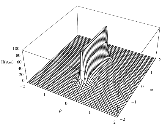
Figure 1: Singularity structure of the warp factor for the $n=4$ geometry in the $(\omega,\rho)$ plane with $l^{2}=-1$.

This deformation corresponds to an $S^{3}$ distribution of D3-branes spanning the locus $\rho=l$ in the $\mathbf{R}^{4}=S^{3}\times\rho$ plane. This is therefore the analytic, canonical form of the $n=4$ metric in [35] which describes an ${\cal N}=4$ field theory with vacuum expectation values for all six scalar fields in the configuration $(2,2,-1,-1,-1,-1)$. The original metric also encodes the $n=2$ solution with scalar vev $(1,1,1,1,-2,-2)$, however this configuration has negative $l^{2}$ as discussed in [35].

The warp factor for the $n=2$ configuration can be plotted in the same way and is illustrated in figure 2.

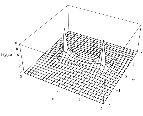
Figure 2: Singularity structure of the warp factor for the $n=2$ geometry in the $(\omega,\rho)$ plane as in figure 1 but with $l^{2}=1$.

This corresponds to a $D^{2}$ distribution spanning the $(\omega_{5},\omega_{6})$ two-plane. It is possible to calculate the canonical, analytic form for the other three metrics in [35] which preserve different subgroups of the original $SO(6)$ symmetry. However, the analytic form for these backgrounds are too complicated to calculate the meson spectra so will be discussed no further.

4 Mesons from D7-Brane Probes

Having found the correct coordinate system in which to describe a canonically normalised field theory living on the D3-branes, we can study the theory with the addition of quarks.

We start with the background described by equation 7 with positive $l^{2}$, which preserves an $SO(4)\times SO(2)$ subgroup of the original symmetry. The D7-brane is embedded by filling the four Minkowski space-time directions, the $\rho$-direction and wrapping the $S^{3}$. This wrapped cycle ensures the stability of the brane configuration.

Before calculating the $x$-dependent excitations of the brane, we must study its flow purely in the $\rho$-direction. This corresponds to calculating $\omega_{5}$ and $\omega_{6}$ as a function of $\rho$. However, because of the supersymmetric nature of this background, the warp factor in front of the $\mathbf{R}^{6}$ is the inverse of that in front of the ${\cal M}^{4}$ plane. This means that the $x$-independent flow is exactly the same as in the $\mathrm{AdS_{5}\times S^{5}}$ background to which the solution is known analytically.

We can solve the equation of motion and obtain the following solutions.

$$\omega=\int\frac{c_{1}}{\sqrt{\rho^{6}-c_{1}^{2}}}d\rho+c_{2}\ ,$$ (9)

where $\omega=\sqrt{\omega_{5}^{2}+\omega_{6}^{2}}$. It is clear that this function will not be real all the way to $\rho=0$ for $c_{1}\neq 0$. The physical solution, corresponding to the renormalisation group flow of the brane, must therefore be $\omega=c_{2}$, equivalent to a quark mass but no quark bilinear condensate. This will always be the case for a supersymmetric solution where the warp factors cancel leaving the $\mathrm{AdS_{5}\times S^{5}}$ equation of motion (excluding $x$-dependent fluctuations).

Because of the manifest $SO(2)$ symmetry between $\omega_{5}$ and $\omega_{6}$, we are free to choose the direction in which to explicitly break this rotational invariance. For simplicity, we choose the solution $\omega_{5}=m$ and $\omega_{6}=0$. We now want to study the mesonic fluctuations about this brane flow. We study the modes in the $\omega_{6}$-direction given by $\omega_{6}=0+\tilde{\omega}_{6}(\rho,x)$. Note that because there is no chiral symmetry breaking in this background, the mesonic excitations in the $\omega_{5}$ and $\omega_{6}$-directions will be identical. This means that the positive and negative parity states will be degenerate.

The action for $\tilde{\omega}_{6}$ up to quadratic order is given by

$$S = \int d^{8}\zeta\rho^{3}\left(\left({\frac{\partial\tilde{\omega}_{6}}{\partial\rho}}\right)^{2}\right.$$

$$+ \left.\left({\frac{\partial\tilde{\omega}_{6}}{\partial x}}\right)^{2}\frac{2R^{4}}{l^{4}+2l^{2}(m^{2}-\rho^{2})+(m^{2}+\rho^{2})^{2}+(l^{2}+m^{2}+\rho^{2})\sqrt{(m^{2}+(l-\rho)^{2})(m^{2}+(l+\rho)^{2})}}\right)\ .$$

For small oscillations about the flow $\omega_{5}(\rho)$, the meson interaction terms will be subdominant and the function $\tilde{\omega}_{6}$ can be treated as a plane wave in the Minkowski space-time directions and therefore the ansatz for this function is given by

$$\tilde{\omega}_{6}=f(\rho)e^{ik.x}\ .$$ (11)

This ansatz which is independent of the three-sphere coordinates corresponds to an $R$-singlet, spinless meson wavefunction. The equation of motion for $f(\rho)$ is given by

$$\frac{2M^{2}\rho R^{4}f(\rho)}{l^{4}+2l^{2}(m^{2}-\rho^{2})+(m^{2}+\rho^{2})^{2}+(l^{2}+m^{2}+\rho^{2})\sqrt{(m^{2}+(l-\rho)^{2})(m^{2}+(l+\rho)^{2})}}+3f^{\prime}(\rho)+\rho f^{\prime\prime}(\rho)=0\ ,$$ (12)

where $M^{2}=-k^{2}$. The eigenvalues, $M$, are given by the values for which the flow of $f$ is well behaved all the way to $\rho=0$ and normalisable in the UV. It must also have the correct scaling dimensions in the $\mathrm{AdS_{5}\times S^{5}}$ limit to describe a mesonic excitation. Of the two UV solutions, the solution corresponding to meson fluctuations, as opposed to an $x$-dependent mass is $f(\rho)\rightarrow\frac{c}{\rho^{2}}$.

It is possible to remove the explicit $R$ and $l$ dependence in the above equation of motion by performing the following rescaling:

$$m=\tilde{m}l,\hskip 14.22636pt\rho=\tilde{\rho}l,\hskip 14.22636ptMR^{2}=\tilde{M}l,$$ (13)

giving us the following equation of motion

$$\frac{2\tilde{M}^{2}\tilde{\rho}f(\tilde{\rho})}{1+2(\tilde{m}^{2}-\tilde{\rho}^{2})+(\tilde{m}^{2}+\tilde{\rho}^{2})^{2}+(1+\tilde{m}^{2}+\tilde{\rho}^{2})\sqrt{(\tilde{m}^{2}+(1-\tilde{\rho})^{2})(\tilde{m}^{2}+(1+\tilde{\rho})^{2})}}+3f^{\prime}(\tilde{\rho})+\tilde{\rho}f^{\prime\prime}(\tilde{\rho})=0\ ,$$ (14)

Before performing this rescaling we can take the $l\rightarrow 0$ limit and find that the numerical values coincide with the known analytic results of the pure $\mathrm{AdS_{5}\times S^{5}}$ spectrum [41]:

$$M=\frac{2m}{R^{2}}\sqrt{(n+1)(n+2)}\ ,\hskip 28.45274ptn=0,1,...$$ (15)

showing that in this limit the numerics are under control. For the rescaled equation (eq.14) we can study the lowest mass meson as a function of the quark mass. Figure 3 shows the value of the first meson mass as a function of the quark mass. The important point to note here is that there appears to be a mass gap in the $m\rightarrow 0$ limit for $l\neq 0$. The numerics make this calculation difficult, though at $m=10^{-10}$ the value of $M_{1}$ is $0.28$. Note that in contrast to the equation of motion with $l=0$, the D7-brane equation is perfectly well behaved in this limit and has discrete eigenvalues. This will be shown analytically in section 4.2.

Figure 3: $M_{1}$ against $\log_{10}m$ for $l=1,R=1$ (solid line). This becomes exactly degenerate with $M_{1}$ for $l=0,R=1$ (dashed line) in the large $m$ limit. Note the appearance of a mass gap. The scale is set by the AdS radius $R$ which can be tuned by hand to compare with lattice data.

Having calculated the first meson mass, we can study the spectrum for the higher excited states. The results of this are shown in figure 4.

Figure 4: $M_{n}$ against $m$ for the first seven states. For large quark masses the behaviour is simple as the brane cannot resolve the double singularity structure, in the small mass limit there is a degeneracy of states. In the large quark mass limit the spectrum goes like $MR^{2}=2m\sqrt{(n+1)(n+2)}$ just as in the pure $\mathrm{AdS_{5}\times S^{5}}$ case.

We can see from figure 4 that there is a degeneracy for quark masses much less than the condensate scale (given by the gap between the singularities in the supergravity geometry). For large quark masses, corresponding to the D7-brane lying far from the singular region, there is a spectrum which is given by

$$MR^{2}=2m\sqrt{(n+1)(n+2)},\hskip 14.22636ptn=0,1,...$$ (16)

as expected because the brane cannot resolve the separated singularities for large quark masses. For smaller masses however we see that pairs of excited states become degenerate and indeed there appears to be an exact degeneracy as we get to the massless limit. The lowest state however does not appear to have a degeneracy and we will show in section 4.2 that this mode does not appear in the exact massless limit when we study the equations analytically.

4.1 Significance of the Canonical Coordinates

It is important at this stage to note why we are interested in finding one particular coordinate system for this problem. Though it appears strange that coordinates matter in what is essentially an eigenvalue problem we see in the following that this canonical coordinate system simplifies the calculations considerably. Without the change of coordinates not only would we be unable to obtain an analytic expression for the meson spectrum in the massless quark limit but because of the numerical behaviour of the supergravity field, $\chi$, we would not be able to obtain a reliable spectrum at all. This means that the numerical instabilities are critical to the eigenvalue problem.

These instabilities stem from two regions in the geometry. The first of these is the singular region where the supergravity field, $\chi$, asymptotes to infinity. The second region is where the space returns to pure $\mathrm{AdS_{5}\times S^{5}}$. In this region the supergravity field asymptotes to unity but the further we go into the ultraviolet, the more significant becomes the accuracy of the solution in insuring a numerically stable geometry. This necessity for ever higher numerical accuracy in the ultraviolet can be seen in equations 3 and 4. In the canonical basis the singular behaviour cancels explicitly in the flow equation for the D7-brane.

The first hint that these instabilities are critical is seen when we calculate the stable value of the quark bilinear condensate as a function of the quark mass. The stable flows of the D7-brane for various quark masses and the quark bilinear condensate versus quark mass are plotted in figures 5 and 6 respectively.

Figure 5: Stable D7-brane flows for varying quark masses. For ease of visualisation the flows are plotted using the coordinates $r^{2}+v^{2}=R^{2}e^{2u}$ and $\frac{v}{r}=\tan{\theta}$ with a singularity at radius $R$.

Figure 6: Quark bilinear condensate versus quark mass calculated from the stable D7-brane flows in figure 5.

In the canonical coordinates we see analytically that there is no condensate present for any quark mass. However, in the original coordinate system (equation 5), we see that for finite $r$ the stable D7-brane solution does not lie flat with respect to the $r$ axis indicating a condensate present for non-zero quark mass. In theory we should be calculating the condensate at infinite energy, where the space returns to pure $\mathrm{AdS_{5}\times S^{5}}$ . This is not possible as we have had to solve the equation numerically. Solving for finite $r$ will always give a non-zero condensate for non-zero quark mass. As we perform the calculation further into the UV where this calculation should be more accurate, the numerical instabilities of the scalar supergravity field become critical and a meaningful result becomes harder to calculate.

When calculating the meson spectrum as a function of the quark mass, the spectrum which is obtained is also found to be a chaotic one, clearly influenced by the singular behaviour in the IR and the numerical instabilities in the UV, especially in the region of small quark mass which is the domain of most interested. This instability is critical to the calculation and means that the interesting properties which can be found analytically and are discussed in the next section are not observable in the original basis using the computational techniques employed here.

4.2 Analytical Results

Though we know from the $m\rightarrow 0$ limit of equation 15 (The $\mathrm{AdS_{5}\times S^{5}}$ meson spectrum) that at $m=0$ the spectrum becomes continuous, this appears not to be the case from the numerical calculation in the $l\neq 0$ deformation. In this case, we can take the $m=0$ limit explicitly in the equation of motion and retain a discrete spectrum.

$$M^{2}\rho R^{4}f(\rho)+l^{2}(l^{2}-\rho^{2})(3f^{\prime}(\rho)+\rho f^{\prime\prime}(\rho))=0\ .$$ (17)

The solution to this equation is given in [35, 36] for the case of the glueball spectrum and is given by:

$$MR^{2}=2l\sqrt{(n+1)(n+2)}\,\hskip 28.45274ptn=0,1,...$$ (18)

(see also [38] for higher angular momentum eigenvalues). It is also precisely the same spectrum as the $\mathrm{AdS_{5}\times S^{5}}$ spectrum with an interchange of the quark mass, $m$ and the deformation parameter, $l$ (the magnitude of the scalar condensate). It is particularly interesting that at this point on the moduli space the spectrum of ${\cal N}=2$ quarks has the same spectrum of states as the ${\cal N}=4$ theory.

There is an apparent discrepancy between the analytical and numerical values calculated in the $m\rightarrow 0$ limit. Interestingly, the masses using the numerical and analytic methods are exactly equal except for the very first state. However, because the infinitesimal and exact massless limits are qualitatively different we may expect a discrete change in behaviour.

For the numerical calculation, in the case, $m=10^{-10}$ and $l=R=1$, the spectrum is given by the values in table 2. The degeneracy is given by the number of mesons with approximately the same eigenvalue.

M	Degeneracy
0.28	1
2.8	2
4.9	2
6.9	2
8.9	2

Table 2: The mass spectrum for $l=R=1$ and $m\rightarrow 0$ calculated numerically. The degeneracy is given by the number of states with converging eigenvalues.

This should be compared with the exact $m=0$ result obtained analytically where the degeneracy is not obtainable. These results are given in table 3.

M	Degeneracy
2.8	n.a
4.9	n.a
6.9	n.a
8.9	n.a

Table 3: The mass spectrum for $l=R=1$ and $m=0$ calculated analytically. The degeneracy is not possible to study in the analytic massless limit because it is not possible to calculate the number of eigenstates of a given eigenvalue.

4.3 The $n=2$ Spectrum

As discussed in section 3 this deformation is obtained from the $n=4$ deformation with the interchange $l^{2}\rightarrow-l^{2}$. This transformation however has a significant effect on the nature of this geometry from the point of view of a D7-brane probe. Again, we can see from the simple product form of the geometry with inverse warp factors for the ${\cal M}^{4}$ and $\mathbf{R}^{6}$ that to zeroth order in mesonic excitations, the D7-branes will lie flat and not notice the singular structure. In figure 2, it was shown that there is a disk singularity lying in the $(\omega_{5},\omega_{6})$ plane of radius $l$. This means that a brane corresponding to adding quarks of mass $m$ for $m<l$ will pass straight through the singular region. We know that this is not a physical configuration and the full interaction between the D3-brane stack and the D7-brane probe would be needed to understand this case fully. It is however possible to study quarks with $m>l$ in the supergravity, probe approximation. We find that as expected, for large masses, the spectrum returns to the $\mathrm{AdS_{5}\times S^{5}}$ values, just as in the large mass limit of the $n=4$ geometry. The spectrum down to $m=l$ is provided in figure 7

Figure 7: $M_{n}$ against $m$ for the first seven states of the $n=2$ deformation for $m>l$ (solid lines).

Though it appears from this diagram that the states may become degenerate (and possibly massless) at $m=l$ this is not apparently the case from these numerical computations, The first seven states are given by the following values at $m=l$:

$$M_{n}=\{1.46,1.59,1.77,2.00,2.26,2.54,2.84\}$$ (19)

In fact the equations are perfectly well behaved for $m<l$ and the spectrum is calculable in this region, however the results should not be trusted as clearly interactions between the D7-brane and the singular D3-brane distribution must be understood fully away from the supergravity limit.

We find that $M_{n}$ is linear in $l$ for $m=l$, though the $n$-dependence is not as simple as the massless $n=4$ geometry. Although the equation of motion simplifies significantly to

$$\frac{2\tilde{M}^{2}f[\tilde{\rho}]}{4+\tilde{\rho}^{2}+\tilde{\rho}\sqrt{4+\tilde{\rho}^{2}}}+3\tilde{\rho}f^{\prime}[\tilde{\rho}]+\tilde{\rho}^{2}f^{\prime\prime}[\tilde{\rho}],$$ (20)

no analytic solution to this equation was obtained.

The qualitative difference between the meson spectrum in this geometry and the $n=4$ case is that there does not appear to be a degenerate spectrum here. The qualitative difference from the point of view of the D7-brane is that there is a continuous distribution of branes rather than a set of singular points with a separation of $2l$.

5 Conclusions

We have found an analytic, canonical form for two scalar deformations formulated in [35]. The singularity structures are exactly as expected from the D3-brane density distribution functions. In these two cases the $SO(6)$ symmetry is broken to $SO(4)\times SO(2)$ which encodes the chiral symmetry of the field theory explicitly, it is possible to calculate the meson spectrum from excitations of probe D7-branes. Interestingly, in one of these backgrounds, it is possible to find the spectrum analytically in the limit of exactly massless quarks. This result includes the existence of a mass gap proportional to the deformation parameter with exactly the same spectrum as the adjoint scalar two point Greens function of the ${\cal N}=4$ theory of [35]. A degeneracy is discovered in the limit of small quark masses (c.f the deformation parameter $l$).

In the second $SO(4)\times SO(2)$ preserving background, it is possible to find the spectra for quarks with larger masses, $m$, than the deformation parameter, $l$. The spectrum in this case does not appear to be degenerate though to fully understand the $m\sim l$ limit, higher order corrections to the supergravity limit must be calculated. The overall conclusion is that by finding the correct analytic, physical coordinates in which to describe the dual gravity theory, we can study the elaborate structure of meson spectra in field theories with complicated condensate terms switched on. If we can do the same thing in the non-supersymmetric analogues of these geometries, we may be able to gain some more insight into real world hadron spectra.

6 Acknowledgements

I would like to thank K Sfetsos for pointing out previous, similar work plus errors in the original version of this paper. I would also like to thank Nick Evans and Feng Wu for helpful discussions and clarification. This project is funded by the Project of Knowledge Innovation Program (PKIP) of the Chinese Academy of Science (CAS).

References

- [1] J. M. Maldacena, Adv. Theor. Math. Phys. 2, 231 (1998) [Int. J. Theor. Phys. 38, 1113 (1999)] [arXiv:hep-th/9711200].
- [2] S. S. Gubser, I. R. Klebanov and A. M. Polyakov, Phys. Lett. B 428, 105 (1998) [arXiv:hep-th/9802109].
- [3] E. Witten, Adv. Theor. Math. Phys. 2, 253 (1998) [arXiv:hep-th/9802150].
- [4] L. Girardello, M. Petrini, M. Porrati and A. Zaffaroni, JHEP 9905, 026 (1999) [arXiv:hep-th/9903026].
- [5] L. Girardello, M. Petrini, M. Porrati and A. Zaffaroni, Nucl. Phys. B 569, 451 (2000) [arXiv:hep-th/9909047].
- [6] K. Pilch and N. P. Warner, Nucl. Phys. B 594, 209 (2001) [arXiv:hep-th/0004063].
- [7] J. Polchinski and M. J. Strassler, arXiv:hep-th/0003136.
- [8] A. Karch and E. Katz, JHEP 0206, 043 (2002) [arXiv:hep-th/0205236].
- [9] A. Karch, E. Katz and N. Weiner, Phys. Rev. Lett. 90, 091601 (2003) [arXiv:hep-th/0211107].
- [10] M. Kruczenski, D. Mateos, R. C. Myers and D. J. Winters, JHEP 0307, 049 (2003) [arXiv:hep-th/0304032].
- [11] T. Sakai and J. Sonnenschein, JHEP 0309, 047 (2003) [arXiv:hep-th/0305049].
- [12] J. Babington, J. Erdmenger, N. J. Evans, Z. Guralnik and I. Kirsch, Phys. Rev. D 69, 066007 (2004) [arXiv:hep-th/0306018].
- [13] C. Nunez, A. Paredes and A. V. Ramallo, JHEP 0312, 024 (2003) [arXiv:hep-th/0311201].
- [14] P. Ouyang, Nucl. Phys. B 699, 207 (2004) [arXiv:hep-th/0311084].
- [15] X. J. Wang and S. Hu, JHEP 0309, 017 (2003) [arXiv:hep-th/0307218].
- [16] S. Hong, S. Yoon and M. J. Strassler, JHEP 0404, 046 (2004) [arXiv:hep-th/0312071].
- [17] N. J. Evans and J. P. Shock, Phys. Rev. D 70, 046002 (2004) [arXiv:hep-th/0403279].
- [18] B. A. Burrington, J. T. Liu, L. A. Pando Zayas and D. Vaman, JHEP 0502, 022 (2005) [arXiv:hep-th/0406207].
- [19] J. Erdmenger and I. Kirsch, JHEP 0412, 025 (2004) [arXiv:hep-th/0408113].
- [20] M. Kruczenski, L. A. P. Zayas, J. Sonnenschein and D. Vaman, JHEP 0506, 046 (2005) [arXiv:hep-th/0410035].
- [21] S. Kuperstein, JHEP 0503, 014 (2005) [arXiv:hep-th/0411097].
- [22] A. Paredes and P. Talavera, Nucl. Phys. B 713, 438 (2005) [arXiv:hep-th/0412260].
- [23] T. Sakai and S. Sugimoto, Prog. Theor. Phys. 113, 843 (2005) [arXiv:hep-th/0412141].
- [24] N. Evans, J. Shock and T. Waterson, JHEP 0503, 005 (2005) [arXiv:hep-th/0502091].
- [25] K. Peeters, J. Sonnenschein and M. Zamaklar, arXiv:hep-th/0511044.
- [26] A. L. Cotrone, L. Martucci and W. Troost, arXiv:hep-th/0511045.
- [27] J. Erlich, E. Katz, D. T. Son and M. A. Stephanov, arXiv:hep-ph/0501128.
- [28] L. Da Rold and A. Pomarol, Nucl. Phys. B 721, 79 (2005) [arXiv:hep-ph/0501218].
- [29] G. F. de Teramond and S. J. Brodsky, Phys. Rev. Lett. 94, 201601 (2005) [arXiv:hep-th/0501022].
- [30] K. Ghoroku, N. Maru, M. Tachibana and M. Yahiro, arXiv:hep-ph/0510334.
- [31] J. Shock and F. Wu, [arXiv:hep-ph/0603142].
- [32] N. Evans and T. Waterson, [arXiv:hep-ph/0603249].
- [33] H. Boschi-Filho and N. R. F. Braga, Eur. Phys. J. C 32, 529 (2004) [arXiv:hep-th/0209080].
- [34] H. Boschi-Filho and N. R. F. Braga, JHEP 0305, 009 (2003) [arXiv:hep-th/0212207].
- [35] D. Z. Freedman, S. S. Gubser, K. Pilch and N. P. Warner, JHEP 0007, 038 (2000) [arXiv:hep-th/9906194].
- [36] A. Brandhuber and K. Sfetsos, Adv. Theor. Math. Phys. 3, 851 (1999) [arXiv:hep-th/9906201].
- [37] K. Sfetsos, JHEP 9901, 015 (1999) [arXiv:hep-th/9811167].
- [38] R. Hernandez, K. Sfetsos and D. Zoakos, JHEP 0603, 069 (2006) [arXiv:hep-th/0510132].
- [39] A. Karch, A. O’Bannon and K. Skenderis, arXiv:hep-th/0512125.
- [40] D. E. Crooks and N. J. Evans, arXiv:hep-th/0302098.
- [41] M. Kruczenski, D. Mateos, R. C. Myers and D. J. Winters, JHEP 0405, 041 (2004) [arXiv:hep-th/0311270].
- [42] J. Babington, N. J. Evans and J. Hockings, JHEP 0107, 034 (2001) [arXiv:hep-th/0105235].