Classical Propagation of Strings across a Big Crunch/Big Bang Singularity

Abstract

One of the simplest time-dependent solutions of M theory consists of nine-dimensional Euclidean space times 1+1-dimensional compactified Milne space-time. With a further modding out by $Z_{2}$, the space-time represents two orbifold planes which collide and re-emerge, a process proposed as an explanation of the hot big bang ekpyrotic ; cyclic ; turok . When the two planes are near, the light states of the theory consist of winding M2-branes, describing fundamental strings in a particular ten-dimensional background. They suffer no blue-shift as the M theory dimension collapses, and their equations of motion are regular across the transition from big crunch to big bang. In this paper, we study the classical evolution of fundamental strings across the singularity in some detail. We also develop a simple semi-classical approximation to the quantum evolution which allows one to compute the quantum production of excitations on the string and implement it in a simplified example.

I Introduction

Recently, an M theory model of a big crunch/big bang transition has been proposed. The model consists of two empty, parallel orbifold planes colliding and re-emerging. Close to the collision, the spectrum of the theory splits into two types of states. The light states are winding M2-branes describing perturbative string theory, including gravity. The massive states, corresponding to higher Kaluza-Klein modes associated with the M theory dimension, are non-perturbative D0-brane states whose masses diverge as the collision approaches. In Ref. turok , it was shown that the equations of motion of the winding M2-branes are regular at the brane collision and yield an an unambiguous classical evolution across it. Since these states describe gravity in quantized string theory, the suggestion is that gravity is better-behaved in this situation than it is in general relativity. If this is true then, rather than seeding a gravitational instability, the massive Kaluza-Klein states may simply decouple around the collision. Provided their density is negligible in the incoming state, as it is in the ekpyrotic and cyclic models ekpyrotic ; cyclic ; wesley , then the entire transition may be describeable using the perturbative string theory states alone.

In this paper, we will assume the massive states can be neglected and focus on the evolution of the fundamental string states across a big crunch/big bang transition of this type. By solving the string evolution equations numerically we show how the higher string modes become excited in a well-defined way as strings cross the transition. We also develop a simple approximation whereby quantum production of excited modes on the string may be computed in a semi-classical manner. Related work may be found in Ref. tolley . Earlier work on strings in cosmological backgrounds is reviewed in Ref. sanchez .

The background space-time we are interested in is most simply understood in eleven-dimensional terms. Near the orbifold plane collision, the line element reduces to that for a $Z_{2}$-compactified Milne universe times $R^{9}$, namely

$$ds^{2}=-dt^{2}+t^{2}d\theta^{2}+\sum_{i=1}^{9}(dx^{i})^{2},$$ (1)

where $0\leq\theta\leq\theta_{0}$, and a $Z_{2}$ reflection is imposed about each end point. For $t<0$ ($t>0$), the two orbifold planes approach (recede) with relative rapidity $\theta_{0}$. Away from the singularity at $t=0$ the space-time is flat and hence an automatic solution of any theory governed by field equations involving purely geometrical terms  geom . At $t=0$ the metric degenerates and the equations of general relativity become singular. Nevertheless, one can analytically continue the background solution through $t=0$. As mentioned, the equations governing the winding M2-branes are regular at $t=0$, so the M2-branes evolve smoothly across the big crunch/big bang transition.

The winding M2-branes reduce to fundamental strings when the M theory dimension is small, so one can also describe the situation in ten-dimensional terms. In string frame, the dimensionally-reduced metric takes the form $g_{\mu\nu}=|t/t_{s}|\eta_{\mu\nu}$, with a time-dependent dilaton, $\phi={3\over 2}{\rm ln}|t/t_{s}|$. Here $e^{\phi}$ is the string coupling and $t_{s}$ is by definition the time when the string coupling is unity  seiberg . For $|t|\ll t_{s}$, stringy interactions are weak and one can, to a first approximation, treat the strings as free. For $|t|$ greater than or of order $t_{s}$, however, the string theory is at strong coupling and one must switch to an eleven-dimensional supergravity description  witten ; ovrut . Recently, techniques for solving the relevant higher-dimensional Einstein equations have been developed paul , which can be applied to this situation. As long as one is considering long-wavelength cosmological perturbations, evolving classically, the transition from the supergravity regime to the string theory ($\alpha^{\prime}$ expansion) regime appears unproblematic: the eleven-dimensional Einstein equations should reduce to the appropriate ten dimensional Einstein-dilaton effective theory as the branes become near. In this paper, our main focus is on the classical dynamics of the string near $t=0$. In a companion paper we provide a complementary treatment, studying the stringy $\beta$ function equations in the usual $\alpha^{\prime}$ expansion to see whether higher order corrections are significant when the string scale crosses the Hubble radius alphacorrections .

In the eleven dimensional picture, there is no dilaton field. The unique mass scale is set by the M2-brane tension $\mu_{2}\equiv M_{11}^{3}$, where $M_{11}$ is the eleven-dimensional Planck mass  tension . Winding membranes, of length $\theta_{0}|t|$ behave like strings with a time-dependent tension, $\mu_{1}=M_{11}^{3}\theta_{0}|t|$, in Minkowski space-time. One can equally well view the strings as having a fixed tension, $\mu_{1}=M_{11}^{3}\theta_{0}|t_{s}|$, but living in a string-frame background metric, $g_{\mu\nu}^{s}=|t/t_{s}|\eta_{\mu\nu}$. The string coupling constant is set by the size of the M theory dimension in eleven-dimensional Planck units: $e^{\phi}=(M_{11}\theta_{0}|t|)^{3\over 2}\equiv|t/t_{s}|^{3\over 2}$.

Starting well away from the collision, at large times $|t|$ the system is described by eleven-dimensional supergravity. As one approaches the collision the string coupling falls below unity, when $|t|$ falls below

$$t_{s}=\theta_{0}^{-1}M_{11}^{-1}.$$ (2)

When $|t|=t_{s}$, the string mass scale is $M_{11}$ and the string length is $l_{s}\sim M_{11}^{-1}\sim\theta_{0}t_{s}$. For small $\theta_{0}$, $l_{s}$ is far smaller than the Hubble horizon scale $t_{s}$ so the characteristic oscillations of the string are little affected by the expansion of the universe. Corrections due to the background space-time curvature are small and the usual $\alpha^{\prime}$ expansion holds good. However, as $|t|$ decreases further, the physical size of an oscillating string remains approximately constant while the physical Hubble radius falls as $|t|(|t|/t_{s})^{1\over 2}$. The string length crosses the Hubble radius at a time

$$t_{X}\sim\theta_{0}^{2\over 3}t_{s}=\theta_{0}^{-{1\over 3}}M_{11}^{-1}.$$ (3)

Thereafter, the string tends towards an ultralocal evolution in which the curvature of the string is unimportant and each bit of the string evolves independently. This is the regime of the $1/\alpha^{\prime}$ expansion discussed in Ref. turok . Figure 1 illustrates the three regimes: from strong to weak coupling at $t_{s}\sim\theta_{0}^{-1}M_{11}^{-1}$ and from flat space to ultralocal evolution at $t_{X}\sim\theta_{0}^{-{1\over 3}}M_{11}^{-1}$. For small $\theta_{0}$, as we shall assume throughout this paper, these times are well-separated.

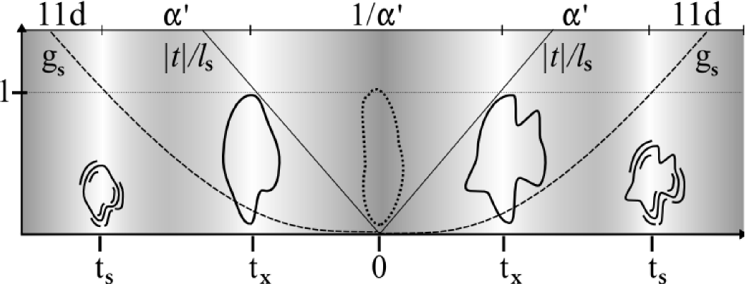
Figure 1: Three phases of an orbifold plane collision, with rapidity $\theta_{0}<1$. Cosmological perturbations are created when the effective theory is the low energy limit of M-theory in eleven dimensions. After the orbifolds get closer and the string coupling ($g_{s}\sim|t/t_{s}|^{3/2}$) falls below unity, the system is better described in terms of perturbative string theory and the usual expansion in $\alpha^{\prime}$. A second transition occurs when the string scale leaves the Hubble radius. Here the string tension becomes dynamically subdominant and the theory is better described by an expansion in $1/\alpha^{\prime}$. In this regime the string is better-described as a collection of independent ‘bits’ whose evolution across the singularity is smooth. After $t=0$ the string tension is reconstituted and the system runs back through the two abovementioned transitions.

In this paper, we wish to study the weak coupling regime, $|t|<t_{s}$, during which the strings cross the singularity. In this regime, for $|t|<t_{X}$, the usual $\alpha^{\prime}$ expansion fails and we must replace it with an expansion in the string tension, proportional to $1/\alpha^{\prime}$. Our ultimate goal is to compute a ‘mini S-matrix’, evolving weakly-coupled incoming string states from an initial time just after $-t_{s}$ to a final time just before $+t_{s}$. In this paper we shall make modest progress towards this goal by computing the ‘mini S-matrix’ in a first, classical approximation.

Any classical solution of the string equations also solves the Heisenberg operator equations for the string field $x^{\mu}(\tau,\sigma)$, to leading order in $\hbar$. For highly excited string states, involving large occupation numbers, the classical approximation should be reasonable. However, to describe gravity we are really more interested in the low-lying states. For these states, quantum corrections are likely to be significant and there is less we can say with precision.

Nevertheless, there are arguments which suggest that quantum corrections may be manageable in the relevant regime. The usual $\alpha^{\prime}$ expansion is based on the approximating space-time as locally flat, and solving the string equations of motion in an expansion in the space-time curvature. This approximation clearly fails to describe even the classical motion of the fundamental strings near $t=0$. Hence the failure of the $\alpha^{\prime}$ expansion in the quantum theory does not, on its own, imply that quantum corrections to the string evolution are largedevega . Second, the key phenomena relevant to the small time regime take place when the background curvature length (i.e. the Hubble radius) falls below the string scale. The string dynamics becomes ultralocal in this regime: in cosmological terms, the string is ‘super-horizon’ and hence may be expected to evolve in a classical manner.

In flat spacetime, the most dramatic consequence of quantizing the string is that the first excited states of the string are massless instead of massive as a classical treatment would suggest. This is due to quantum mechanical renormalization of the mass squared operator, $m^{2}=(p^{0})^{2}-\vec{p}^{2}$, where $p^{\mu}$ is the string’s centre of mass momentum. The renormalized mass squared operator is lowered by one quantized unit relative to the normal ordered classical expression, and this lowering causes the first excited states to become massless. As a result, the string centre of mass trajectory $x_{cm}^{\mu}=q^{\mu}+p^{\mu}\tau$ is altered from the classical expression by $(p^{0})^{2}\rightarrow(p^{0})^{2}-M^{2}$ with $M$ a constant so that the quantum corrected trajectory is null instead of spacelike. Note, however, that this shift in the energy $p^{0}$ merely alters the time coordinate of the centre of mass of the string and it does not affect the string spatial coordinates and momenta, which obey exactly the same equations as in the classical theory. Again, this discussion suggests that quantum effects may be relatively modest in the situation we are interested in.

In this paper, we focus on the classical evolution of the string across $t=0$. Starting at a time $t$ of order $-t_{s}$, we expect the string to oscillate nearly adiabatically and with almost fixed physical size until the string scale crosses the Hubble radius at time $t=-t_{X}$. For small $\theta_{0}$, $t_{s}\gg t_{X}$, hence there is a large range of time over which adiabatic evolution holds. This allows us to clearly identify the incoming and outgoing states in terms of the usual flat space-time modes. As we have already mentioned, the natural size scale for the incoming states we are interested in (i.e. the graviton, dilaton or antisymmetric tensor states) is the string scale at $t_{s}$,

$$\Delta x\sim\ M_{11}^{-1}\sim\theta_{0}t_{s}.$$ (4)

By the same token, the natural measure for the spatial momentum of the string state at this time is

$$P\sim M_{11}\sim(\theta_{0}t_{s})^{-1},$$ (5)

and we shall always measure the momentum of the incoming string in this basic units.

One of the nice features of the problem at hand is that the string tends to simple flat space evolution at large asymptotic times:

$$x^{\mu}(\tau,\sigma)\rightarrow\,^{(in)}\!\,\,\!x^{\mu}(\tau,\sigma)\qquad t\rightarrow-t_{s},$$ (6)

and

$$x^{\mu}(\tau,\sigma)\rightarrow\,^{(out)}\!\,\,\!x^{\mu}(\tau,\sigma)\qquad t\rightarrow+t_{s},$$ (7)

where ${}^{in}x^{\mu}(\tau,\sigma)$ and ${}^{out}x^{\mu}(\tau,\sigma)$ are free string fields evolving adiabatically in the usual flat space string modes. The limits should, strictly speaking, be expressed in terms of a $t_{c}<t_{s}$ so that we are always studying times for which the string coupling is smaller than unity. In practice this will not be an important distinction since as long as $\theta_{0}$ is small, the string states we study tend to their asymptotic behavior at times $t_{X}\ll t_{s}$.

In a linear field theory in a time-dependent background, where the field tends to the usual Minkowski evolution in the asymptotic past, all of the information regarding quantum amplitudes may be obtained from real solutions of the classical field equations (see e.g.  birrell ). One simply expresses the incoming field as a linear combination of creation and annihilation operators, defined by their action on the incoming vacuum state, multiplied by the appropriate positive and negative frequency modes. The classical field equations then determine the quantum Heisenberg field for all time. Using the time-dependent field, one can then compute any correlation function of interest, evaluated in any incoming state expressed in terms of incoming creation operators acting on the incoming vacuum.

The main difference in our situation is that the string evolution is nonlinear. Nevertheless, the nonlinearity turns out to be of a very simple form, where one can apply a semi-classical approximation in a self-consistent way. One can follow a similar procedure to that in the linear case to compute the quantum production of string excitations due to passage across the singularity. We shall explain this calculation, for a specially simple case – a circular loop – in the final section of this paper. The calculation may be generalized to higher modes of the string and we shall do so in a future publication.

The outline of this paper is as follows. In section II we present the equation governing winding membranes, discuss their adiabatic solutions and define various quantities of interest. In section III we study the classical evolution of a circular loop, representing the dilaton and its massive counterparts. In section IV we study the classical evolution of a rotor, representing the modes of maximal spin (for example, the graviton), at each mass level. Section V describes the classical evolution of a state of intermediate angular momentum, representing an antisymmetric tensor state and massive analogs. Section VI gives an example of a quantum transmutation amplitude computed for an incoming dilaton-like state. In section VII we give a brief summary with future proposals. In Appendix A we give an analytic solution method for the classical string equations, representing an expansion in powers of the string tension, i.e., inverse powers of $\alpha^{\prime}$, which accurately describes the passage of a circular loop across the singularity. Intriguingly, in this regime polylogarithm functions enter, perhaps hinting at some deeper analytic solution yet to be found. We also present an analytic solution to second order in $1/\alpha^{\prime}$ for a more general string configuration. Finally, Appendix B is devoted to some numerical checks on the right/left mover decomposition for the special case of a classical rotor.

II Equations of motion for a winding membrane

Our starting point is the Nambu-Goto action for a membrane,

$${\cal S}=-\mu_{2}\int d^{3}\sigma\sqrt{-\mathrm{Det}(G^{(3)}_{ab})},$$ (8)

where $\sigma^{a}$ ($a=0,1,2$) are the three world-volume coordinates, $G_{ab}\equiv\partial_{a}x^{A}\partial_{b}x^{B}g_{AB}$ is the induced metric on the world-volume, $x^{A}=(t,\vec{x},y)$ are the space-time embedding coordinates and $\mu_{2}$ is the membrane tension. For a winding membrane in its lowest Kaluza-Klein state, we can set $\sigma^{2}=\theta$ in the Milne metric (1). The action (8) then reduces to

$$S=-\mu_{2}\int\theta_{0}|t|d^{2}\sigma\sqrt{-\mathrm{Det}(G^{(2)}_{\alpha\beta})},$$ (9)

where now $G^{(2)}_{\alpha\beta}$ is the induced metric on the two-dimensional world sheet with coordinates $\sigma^{0}\equiv\tau$ and $\sigma^{1}\equiv\sigma$. Henceforth dots shall denote derivatives with respect to $\tau$ and primes derivatives with respect to $\sigma$.

The action (9) may be viewed as describing a string moving in flat space-time with a tension $\mu_{2}\theta_{0}|t|$ tending to zero as the string approaches the singularity. Hence one expects all points on the string to move with the speed of light in this limit. Equivalently, the same action may be viewed as describing a string of fixed tension $\mu_{2}\theta_{0}t_{s}$, moving in a time-dependent background with metric $g_{\mu\nu}=|t/t_{s}|\eta_{\mu\nu}$. We shall adopt this latter point of view throughout the paper.

The action (9) is invariant under reparametrizations of the string world sheet. In particular, we can choose timelike gauge $x^{0}\equiv t=\tau$, and also $\dot{\vec{x}}\cdot\vec{x}\,^{\prime}=0$. In this gauge, the string spatial coordinate $\vec{x}(t,\sigma)$ obeys the following classical equations of motion:

$$\partial_{t}\big{(}\epsilon\dot{\vec{x}}\big{)}=\partial_{\sigma}\Big{(}\frac{t^{2}\partial_{\sigma}\vec{x}}{\epsilon}\Big{)},\qquad\partial_{t}\epsilon = t\frac{(\vec{x}^{\prime})^{2}}{\epsilon},$$ (10)

where $\epsilon$ is an auxiliary quantity (roughly speaking, the ‘relativistic energy density’ for the string), defined by

$$\epsilon=\sqrt{\frac{t^{2}(\vec{x}^{\prime})^{2}}{(1-{\dot{\vec{x}}}\,^{2})}}.$$ (11)

Equations (10) and (11) imply that

$$\partial_{t}(\epsilon^{2})=\frac{2}{t}(1-\dot{\vec{x}}\,^{2})\,\epsilon^{2},$$ (12)

which will be useful later. Notice in particular that as $t$ tends to zero, from (10) $\epsilon$ tends to a constant. Hence from from (12) the speed of the string tends to unity. As pointed out in Ref.  turok , for generic string states, equations (10) are regular for all $t$.

As in flat space-time, it is useful to rewrite these equations in terms of left and right moving modes, defined by

$$\vec{r}=\dot{\vec{x}}-\frac{|t|}{\epsilon}{\vec{x}}\,^{\prime},\qquad\qquad\vec{l}=\dot{\vec{x}}+\frac{|t|}{\epsilon}{\vec{x}}\,^{\prime}.$$ (13)

It is easy to show that $\vec{l}$ and $\vec{r}$ are unit vectors, $\vec{r}\,^{2}=1=\vec{l}\,^{2}$, as in flat space kibble . For a closed string, they each describe a closed curve on a unit sphere. Notice also that whereas the timelike gauge we have chosen is invariant under reparameterizations of $\sigma$, the the left and right movers are themselves reparameterization invariant. Many of the properties of oscillating loops can be seen most directly by picturing the left and right movers as curves on a unit sphere. In three spatial dimensions, even in flat space-time such curves generically cross. Where this happens the left and right movers coincide, and it follows that the string moves at the speed of light for an instant  ntnpb . As we have already mentioned, in the background of interest, at $t=0$ every point on the string must move at the speed of light. Hence, at this moment, the the left and right mover curves must actually coincide.

In terms of the left and right movers, the equations of motion (10) read

$$\dot{\vec{r}}+\frac{|t|}{\epsilon}\vec{r}\,^{\prime}+\frac{1}{2t}\left(\vec{l}-(\vec{r}\cdot\vec{l})\vec{r}\right) = 0,$$

$$\dot{\vec{l}}-\frac{|t|}{\epsilon}\vec{l}\,^{\prime}+\frac{1}{2t}\left(\vec{r}-(\vec{r}\cdot\vec{l}).\vec{l}\right) = 0.$$ (14)

In the limit $t\rightarrow 0$, the last terms in each equation force

$$\vec{r}\rightarrow\vec{l},$$ (15)

so that, as explained earlier, all points on the string reach the speed of light. Conversely, in the limit of large times, when a loop is well inside the Hubble horizon, one expects it to evolve as in flat space-time. As explained below, when we convert to proper time and space coordinates, the right and left movers defined in (13) correspond to flat space-time right and left movers after a reparameterization of $\sigma$. Our numerical calculations verify that $\vec{r}$ and $\vec{l}$ tend towards fixed curves at large times, providing a straightforward matching onto flat space-time solutions in this asymptotic regime.

The equations of motion are non-linear and hard to solve analytically. We have therefore resorted to a numerical study of a variety of cases. We have also developed analytic approximations in the large time and small time limits, which we compare to the numerical results. Recall that the string length is $\sim M_{11}^{-1}$ when we start our evolution, and the Hubble radius is larger by a factor $\theta_{0}^{-1}$. As time runs forward, the comoving Hubble radius shrinks as $|t|$ and the comoving loop size grows as $|t/t_{s}|^{-{1\over 2}}$. Once the string crosses the Hubble radius, its vibrations cease and the string follows a kinematical super-Hubble evolution.

The ‘freezing’ of the string outside the Hubble radius is, as we will discuss below, like a sort of measurement process. Depending on the phase of oscillation of the string, either the string coordinate can be frozen, or its momentum. In either case, the conjugate variable then acquires a large kick following $t=0$. After crossing the singularity, the loop re-enters the Hubble radius and starts oscillating as in flat space once again (see Figure 1).

II.1 Asymptotic states: flat space description

At early and late times the string loop is well inside the Hubble radius and we expect it to follow standard flat space-time evolution, which we now pause to review. In standard flat coordinates,

$$ds_{fl}^{2}=-dT^{2}+(d\vec{X})^{2},$$ (16)

we can choose timelike, orthonormal gauge, $T=\tau$ and $(\partial_{T}\vec{X})\cdot(\partial_{\sigma}\vec{X})=0$. The string then evolves according to the wave equation

$$\partial_{T}^{2}\vec{X}=\partial_{\sigma}^{2}\vec{X},$$ (17)

with the constraint

$$(\partial_{T}\vec{X})^{2}+(\partial_{\sigma}\vec{X})^{2}=1.$$ (18)

The usual left and right movers are given by

$$\vec{R}=\partial_{T}\vec{X}-\partial_{\sigma}\vec{X},\qquad\qquad\vec{L}=\partial_{T}\vec{X}+\partial_{\sigma}\vec{X},$$ (19)

and the equations of motion may be written

$$\partial_{T}\vec{R}+\partial_{\sigma}\vec{R}=0,\qquad\qquad\partial_{T}\vec{L}-\partial_{\sigma}\vec{L}=0.$$ (20)

The solutions may be expressed as a sum over Fourier modes,

$$R^{i}(T-\sigma)=\sum_{n=-\infty}^{+\infty}\alpha^{i}_{n}e^{-in(T-\sigma)},\qquad\qquad{L}^{i}(T+\sigma)=\sum_{n=-\infty}^{+\infty}\tilde{\alpha}^{i}_{n}e^{-in(T+\sigma)},$$ (21)

where reality imposes $(\tilde{\alpha}^{i}_{n})^{*}=\tilde{\alpha}^{i}_{-n}$ and ${(\alpha_{n}^{i})}^{*}=\alpha^{i}_{-n}$. To quantize the string, these Fourier parameters are promoted to operators. After following the canonical procedure, and regularizing and renormalizing the nonlinear constraints, one finds there are three massless excitations, consisting of states of the form $\alpha_{-1}^{\mu}\tilde{\alpha}_{-1}^{\nu}|0\rangle$ where $|0\rangle$ is the oscillator vacuum state. These states consist of a space-time scalar (the dilaton), a symmetric and traceless tensor (the graviton) and an antisymmetric tensor. These modes are the most relevant cosmological perturbation theory and evolving perturbations through the bounce. Hence, the rest of the paper will be dedicated to their classical analogs. We shall not, however, study the important issue of mass renormalization, which we defer to future work.

The classical string configuration with no angular momentum, hence corresponding to a dilaton-like state, consists of a circular loop. In its rest frame, a loop in the $XY$ plane takes the form:

$$\vec{X}_{D}=\mathrm{cos}(T)\bigl{(}\mathrm{cos}(\sigma),\mathrm{sin}(\sigma),0,\dots,0\bigr{)},\qquad 0<\sigma\leq 2\pi.$$ (22)

In contrast, the state with maximal angular momentum for a given energy, analogous to the graviton, takes the form of a rotor, a spinning doubled line:

$$\vec{X}_{G}=\mathrm{cos}(\sigma)\bigl{(}\mathrm{cos}(T),\mathrm{sin}(T),0,\dots,0\bigr{)},\qquad 0<\sigma\leq 2\pi.$$ (23)

The left and right movers are easily calculated: they are circles in the $XY$ plane which are parallel in the case of the dilaton-like state and antiparallel in the graviton-like state. A state of intermediate angular momentum may be constructed by taking the left and right movers to trace out two circles in perpendicular planes. Choosing the right mover in the $XY$ plane, and the left mover in the $XZ$ plane, the classical solution is

$$\vec{X}_{A} = \frac{1}{2}\Big{(}\,2\,\mathrm{cos}(T)\mathrm{sin}(\sigma),\,\mathrm{cos}(T-\sigma),\,\mathrm{cos}(T+\sigma),\,0,\dots,\,0\,\Big{)},$$ (24)

The three solutions and their description in terms of left and right movers on the sphere are depicted in Figure 2.

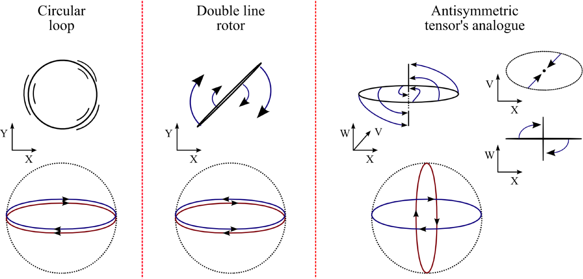
Figure 2: Classical flat space-time solutions consisting of the lowest mode excitations with minimal, maximal and intermediate angular momentum. To get zero angular momentum the right and left movers lie in the same plane with parallel orientation. This configuration corresponds to an oscillating circular loop. The solution with maximal angular momentum is similar but has the left and right movers oppositely oriented. This solution describes a spinning doubled line, or rotor. A classical solution with intermediate angular momentum is achieved by taking the right mover circle to lie in a plane orthogonal to the left mover circle. The solution is three-dimensional. However, under a suitable projection it appears as an elliptical loop, spinning through an intermediate doubled-line configuration. The $WV$ plane is spanned by $\hat{V}=(0,1,1,0,...,0)/\sqrt{2}$ and $\hat{W}=(0,-1,1,0,...,0)/\sqrt{2}$.

In order to connect these flat space-time solutions to those solutions in an expanding universe, we need to relate comoving coordinates $\vec{x}$ and conformal time $t$ to physical coordinates $\vec{X}$ and proper time $T$. Since $d\vec{X}=a\,d\vec{x}$ and $dT=a\,dt$, the factors of the scale factor $a$ cancel out in the velocity. One can also show, using the result of Ref.  turokv2 that the time-averaged velocity squared of a loop in its center of mass frame is ${1\over 2}$, that (12) implies that $\int\epsilon d\sigma\propto|t|^{1\over 2}\propto a(t)$. Using this result, one can show using an appropriate reparameterization of $\sigma$ that the left and right movers (13) map precisely onto the flat space left and right movers (19). This makes it easy to send in states of any desired asymptotic form, and to read off the states in which they come out. A further convenience of the timelike orthonormal gauge we use is that we do not need to actually perform the reparameterization of $\sigma$. At any value of $\sigma$ one can read off the left and right movers as functions of the time $t$.

II.2 Conventions and important quantities for the incoming/outcoming modes

As noted above, we will generally choose $\sigma$ to run from 0 to $2\pi$. Moreover, in our convention capital letters (like $X$, $E$, etc.) denote flat space-time quantities, i.e. those which correspond to flat space-time variables in the regime where the expansion of the universe is adiabatic (i.e. where the string loop is well inside the Hubble radius). On the other hand, lower case symbols (like $x$, $\epsilon$, $t$, etc) describe coordinates or quantities in the cosmological background. To specify an incoming mode, for the circle or rotor we will assume the initial string configuration is in the $xy$ plane, with some center of mass velocity in the $z$ direction. We define the latter by

$$v_{z}=\frac{\int\epsilon\,\dot{{z}}\,d\sigma}{\int\epsilon\,d\sigma},$$ (25)

calculated at a time where we start the evolution, which we shall formally denote $-t_{s}$. The flat space solutions used to specify initial conditions are obtained by Lorentz boosting those given above. Moreover, we will define the comoving string size at $t_{s}$ to be

$$\Delta x=\frac{1}{2\pi}\int d\sigma|\vec{x}\,^{\prime}|.$$ (26)

and we shall choose this to be unity in the initial state. For each choice of the initial time $t_{s}$, there will be an associated orbifold rapidity $\theta_{0}=t_{s}^{-1}$. Finally, to get a quantitative measure of how much energy was produced (or lost) during the $t=0$ transition, one can define a flat-space-time energy

$$E=\int d\sigma\epsilon\,|t_{s}t|^{-1/2}$$ (27)

which approaches a constant for large values of $|t|$, as explained above. The energy ratio between an incoming mode and an outgoing one ($\eta=E_{in}/E_{out}$) provides a measure of how much energy was produced during the string’s passage across the singularity.

We will now consider separately the behavior of the circle, the rotor and the classical analog of the antisymmetric tensor.

III Circular loop

The simplest nontrivial case to study is a circular loop, where the symmetry reduces the problem to a single dynamical variable. Employing the symmetric ansatz $\vec{x}(\tau,\sigma)=\rho(\tau)\left(\,\cos(\sigma),\,\sin(\sigma),\,0,...,0\,\right)$ where $\rho$ is the comoving radius of the loop, in the gauge $t=\tau$ the string action (9) reduces to

$${\cal S}=-2\pi\mu_{2}\int dt\theta_{0}|t||\rho|\sqrt{1-\dot{\rho}^{2}}.$$ (28)

To minimize clutter, from now on we shall work in time and length units in which $2\pi\mu_{2}\theta_{0}=1$. The canonical momentum $p$ conjugate to $\rho$ and the Hamiltonian are found respectively to be

$$p={d\rho\over dt}{|t|S|\rho|\over\sqrt{(1-\dot{\rho}^{2})}},\qquad H=\epsilon=\sqrt{p^{2}+t^{2}\rho^{2}},$$ (29)

and Hamilton’s equations are

$${dp\over dt}=-{t^{2}\,\rho\over H},\qquad{d\rho\over dt}={p\over H}.$$ (30)

Finally, because the Hamiltonian is expicitly time-dependent, we obtain

$${dH^{2}\over dt}=2t\rho^{2}.$$ (31)

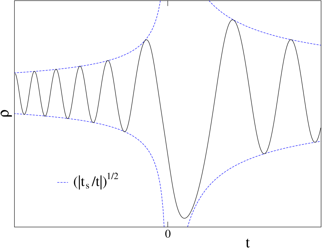
Figure 3: Numerical solution to equations (29)-(31). For large $|t|$, the comoving radius $\rho$ oscillates, with an envelope growing as $|t_{s}/t|^{1/2}$. The evolution across $t=0$ is smooth and, in this particular example, it results in a larger amplitude oscillation after the transition.

The qualitative properties of the solutions to (29)-(31) are easily seen. The energy density $\epsilon=H$ takes its minimal value at $t=0$, where the radial speed $d\rho/dt$ reaches unity. This last effect triggers interesting effects which we shall describe below. The solutions are regular for all $t$ except for the special case where the momentum $p$ vanishes at $t=0$. For that case, (31) implies that $H\sim\rho_{0}|t|$ at small $t$. From (30) and (29), one finds that $p$ is very mildly non-analytic, $p\sim-{1\over 2}t^{2}{\rm sign}(t)$, whereas $\rho\sim\rho_{0}-{1\over 4}t^{2}/\rho_{0}$ is regular.

Equations (29)-(31) are invariant under the rescaling $t\rightarrow\Lambda t$, $\epsilon\rightarrow\Lambda^{2}\epsilon$, $p\rightarrow\Lambda^{2}p$ and $\rho\rightarrow\Lambda\rho$, hence solutions for loops of different sizes are trivially related, and inequivalent solutions are labelled by only one parameter, which may, for example, be taken to be the asymptotic phase of the oscillation.

The motion of the loop is simplest to describe in two asymptotic regimes, corresponding to large and small $|t|$, when the loop’s radius $\rho$ is well within, or outside, the Hubble radius. In the first regime the loop oscillates with fixed amplitude and period in proper time. In comoving coordinates and conformal time the oscillation amplitude changes as $a(t)^{-1}=(t_{s}/|t|)^{1/2}$, and the frequency changes as $a(t)\propto(|t|/t_{s})^{1/2}$, as illustrated in Figure 3. The energy density $\epsilon$ scales as $a(t)=(|t|/t_{s})^{1/2}$ in this regime.

Once the comoving Hubble radius $|t|$ falls below the loop radius $\rho$, the loop enters a new kinematical regime in which the tension plays a subdominant role. As the time tends to zero, all points on the string approach the speed of light. The loop receives a ‘kick’ from passing through $t=0$ and emerges with a shift in its its oscillation phase and a net energy gain or loss. In the case of a circular loop, if the radius is expanding at $t=0$ the loop gains energy, whereas if it is contracting the loop loses energy. Time reversal, which is a symmetry of the equations, relates these two situations. Figure 4 shows two examples.

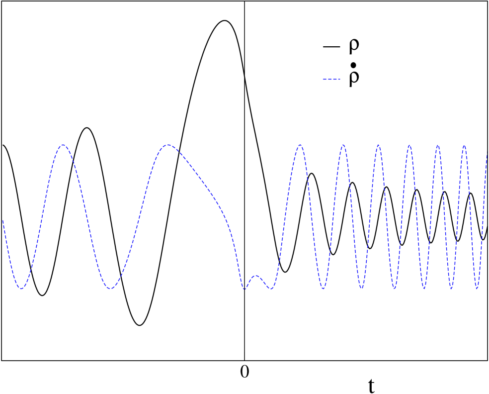
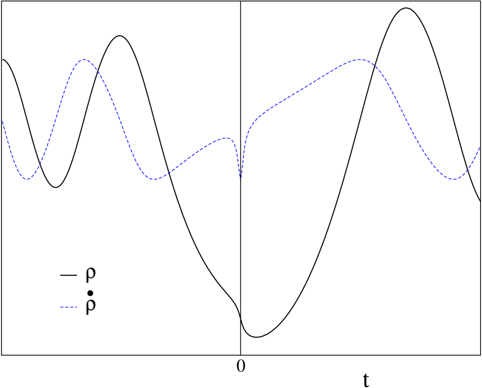
Figure 4: The radius (solid black line) and the velocity (blue dashed line) are plotted for two different circular loops. In the left plot the singularity is crossed after a maximum in the radius and almost at a minimum in the velocity. In this particular case, there is a loss of energy after the transition: the outgoing mode has a smaller amplitude than the incoming one. The right plot shows the opposite situation, with the radial coordinate approaching a maximum at the singularity, and energy being produced.

III.1 Asymptotic states at large $|t|$

In order to parameterize the incoming and outgoing states, it is helpful to perform a canonical transformation to new coordinates ($\phi,\,\mathcal{P}$):

$$\mathcal{P}=\frac{p^{2}+t^{2}\rho^{2}}{2|t|},\qquad\qquad\tan(\phi)=\frac{\rho|t|}{p}.$$ (32)

At large times, the angle $\phi$ represents the oscillation phase while the conjugate momentum $\mathcal{P}$ tends to a constant measuring the energy stored in the loop. The Hamiltonian equations now read

$${d{\mathcal{P}}\over dt} = -\frac{\mathcal{P}}{t}\cos(2\phi),$$

$${d{\phi}\over dt} = \sqrt{\frac{|t|}{2\mathcal{P}}}+\frac{1}{2t}\sin(2\phi).$$ (33)

These equations are readily solved at large times, giving

$$\mathcal{P}\rightarrow\mathcal{P}_{\infty}=\mathrm{const.},\qquad\qquad\phi\rightarrow\int\sqrt{\frac{t}{2\mathcal{P}}}dt\sim\pm\frac{2}{3}\sqrt{\frac{|t|^{3}}{2\mathcal{P}_{\infty}}}+\phi_{0},$$ (34)

where $\phi_{0}$ is a constant phase. From (32) it follows that the energy (27) $E\propto\sqrt{\mathcal{P}}$ and hence it tends to a constant at large times, as expected. In the usual comoving $\rho$ coordinate, the asymptotic behavior of the solution at large times is

$$\rho\sim\sqrt{\frac{2\mathcal{P}_{\infty}}{t}}\sin\left(\frac{2}{3}\sqrt{\frac{t^{3}}{2\mathcal{P}_{\infty}}}+\phi_{0}\right).$$ (35)

Upon identifying proper time and radius, this takes the form of the flat space solution (22), up to an arbitrary phase. Due to the rescaling symmetry discussed above, the only nontrivial parameter in the incoming state is the phase $\phi_{0}=\phi_{in}$. The outgoing state may be completely characterized by a similar phase $\phi_{out}$, and by the energy ratio $\eta=E_{in}/E_{out}$, both of which can be expressed as a function of the incoming phase. Figure 5 shows all the information needed to describe the classical transition, i.e., the outgoing energy and phase in term of similar ingoing quantities. In the case of the energy ratio $\eta$, one can determine the energy production for an incoming mode with fixed amplitude but unknown phase, or equivalently, the average energy production weighted by the Liouville measure. By integrating the curve in Figure 5, we find

$$<\eta>=\frac{1}{2\pi}\int_{0}^{2\pi}\eta\ d\phi_{in}=2.12.$$ (36)

Before moving into the regime close to the singularity let us briefly comment on the consequences of including a non-zero center of mass velocity. As we increase the initial center of mass velocity $v_{z}$, the energy production decreases so that the plot for $\eta$ (Figure 5) shrinks in the vertical direction. This is to be expected since the $z$ component of the string’s velocity means that it is closer to the speed of light and hence suffers less of a ‘kick’ as it passes through $t=0$. This translates into less energy production or energy loss.

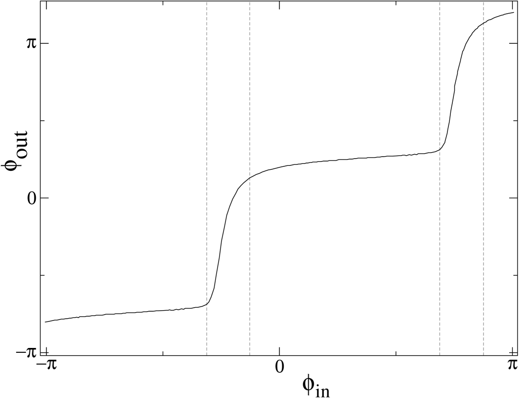
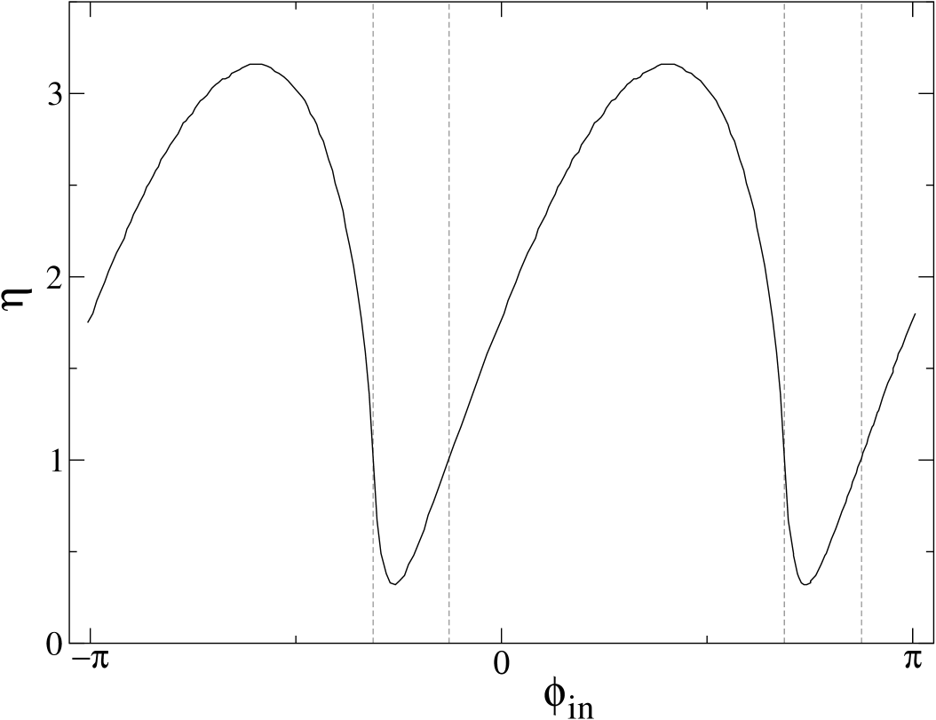
Figure 5: The outgoing phase $\phi_{out}$ measured at large times is shown as a function of the incoming phase $\phi_{in}$ (left plot). There are two different regions, one where $\phi_{out}$ varies steeply and the other where it is almost flat. The right hand plot shows the energy production ratio $\eta=E_{out}/E_{in}$ as a function of the incoming phase $\phi_{in}$. The ratio $\eta$ is less than one in the steep region of the left hand plot, and greater than one outside it. Two neighboring regions are related by time-reversal (which sends $\eta$ to $1/\eta$), and they are separated by special points at which $\eta=1$. These special points, denoted by the vertical dashed lines, correspond to the loop crossing $t=0$ with either zero momentum or zero radius.

III.2 Behavior near the singularity

Classically, the state of a circular loop with zero center of mass velocity is specified by two numbers, its radius and the canonically conjugate momentum. However because of the scaling symmetry discussed above, there is really only one physical parameter. Near the singularity, we can choose the scale-invariant combination $|p_{0}/\rho_{0}^{2}|$, where $p_{0}$ and $\rho_{0}$ are the values of $p(t)$ and $\rho(t)$ at $t=0$. This combination compares the radial momentum to the size of the loop at the singularity: if $|p_{0}/\rho_{0}^{2}|\ll 1$, then the radius is large and not much changed during the transition across the singularity. In contrast, if $|p_{0}/\rho_{0}^{2}|\gg 1$, then the momentum is hardly changed during the transition. In each case, the conjugate variable undergoes a large change across the transition. Heuristically, one can think of the transition as ‘measuring’ the loop radius or its momentum in the two cases, so that the conjugate variable acquires a large jump, as a consequence of Liouville’s theorem. Figures 6 and 7 illustrate the two situations. The former situation, where the radius is ‘frozen’ during the transition, describes the rising portion of the $\eta(\phi_{in})$ curve in Figure 5. As can be seen from the plot, this is the more common situation for initial states with uniformly chosen $\phi_{in}$.

Likewise, certain features of Figure 5 are readily understood. Recalling that the phase $\phi$ and the ‘energy’ $\mathcal{P}$ defined in (32) are canonically conjugate, one sees how the squeezing of the outgoing phase causes the loop energy to be amplified, and vice versa.

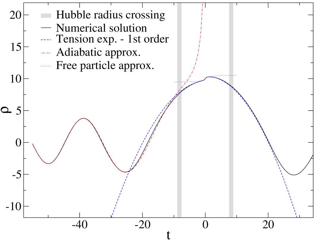
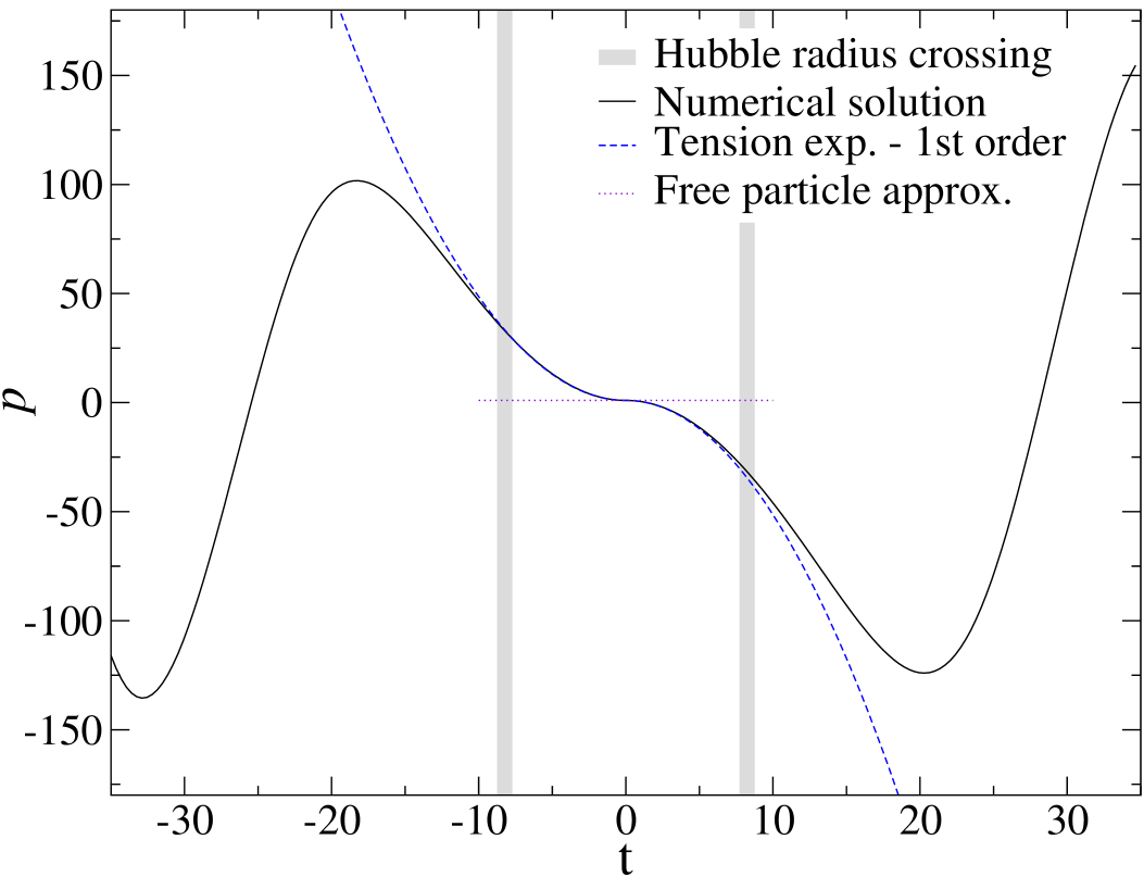
Figure 6: Both numerical simulations and analytical approximations for the radius $\rho$ (left plot) and the canonical momentum (right plot) are shown as a function of time for a circular loop. Due to the small invariant parameter $|p_{0}/\rho_{0}^{2}|=0.1$, it is the loop radius (left plot), not the momentum (right plot) that ‘freezes’ during the transition. The expansion in the string tension (see text) works well in this case, even beyond Hubble crossing. In contrast, the free particle approximation only agrees with the numerics close to $t=0$, where there is drastic change in the string momentum. If the loop radius is taken to be of order the string length $l_{s}$ at a time $t_{s}$, then this case corresponds to $\theta_{0}\sim 1/260$.

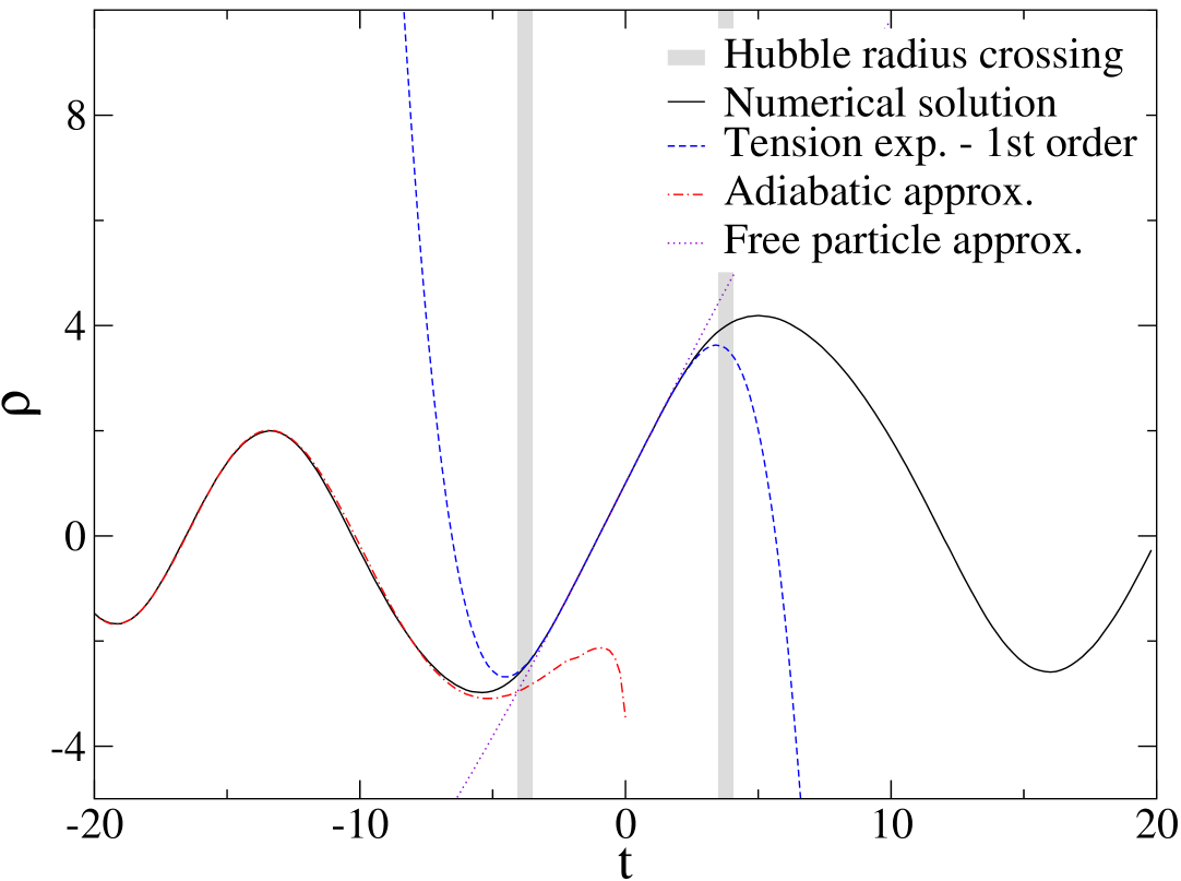
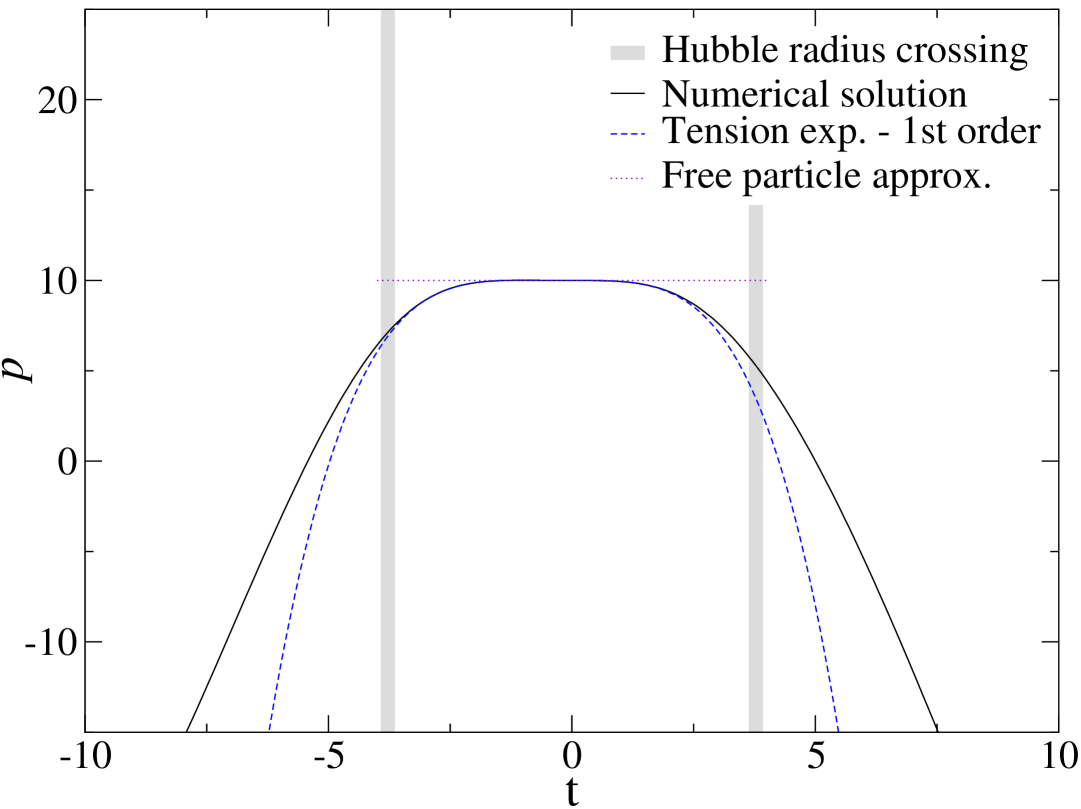
Figure 7: Another circular loop example, where in contrast to the situation in Figure 6, the ratio $|p_{0}/\rho_{0}^{2}|=10$ so that the momentum $p$ is nearly frozen across the transition, whereas the radius $\rho$ changes significantly - undergoing a complete oscillation. In this case, the expansion in the string tension works only until Hubble crossing, and describes the maximum and minimum with less precision. If the loop radius is taken to be of order the string length $l_{s}$ at a time $t_{s}$, then this case corresponds to $\theta_{0}\sim 1/128$.

III.3 Analytical treatment: an expansion in the string tension

To understand the behavior near the singularity better, we consider expanding about $t=0$. The simplest possibility is merely to perform a Taylor series in $t$, but this expansion is poorly convergent. Instead, we have developed an analytic solution method which is formally an expansion in the string tension, or $1/\alpha^{\prime}$.

To perform this expansion, let us introduce a formal parameter $\lambda$ multiplying the tension term in the Hamiltonian, so that

$$H\rightarrow\sqrt{p^{2}+\lambda t^{2}\rho^{2}}.$$ (37)

We now calculate the Hamiltonian equations as before, using (37) to eliminate the $\lambda$-dependence of the equation for the time-dependence of the Hamiltonian. We obtain

$${dp\over dt}=-\lambda{t^{2}\,\rho\over H},\qquad{d\rho\over dt}={p\over H},\qquad{dH^{2}\over dt}={2\over t}(H^{2}-p^{2}).$$ (38)

In this form, $\lambda$ appears in only one term in the equations of motion. We can solve the equations as a power series in $\lambda$ by inserting the lower order solution into the term involving $\lambda$ at each new order. At the end of the calculation, we set $\lambda=1$ and fix all remaining integration constants. Notice that we do not allow powers of $\lambda$ in the initial conditions: the approximation applies only to the dynamical evolution.

The zeroth order solution is found by setting $\lambda=0$ in equations (38). The first equation implies $p=p_{0}$, a constant. The last equation then implies $H=\sqrt{p_{0}^{2}+C^{2}t^{2}}$, with $C$ a constant. Finally, the equation for $\rho$ is easily integrated. Finally, we set $\lambda=1$ and identify the integration constant $C$. Comparing the expression for $H$ in our solution with the exact Hamiltonian, we can see that $C=\rho_{0}$, the radius of the loop at $t=0$. Hence we obtain the zeroth order solution

$$\rho=\rho_{0}+\frac{p_{0}}{\rho_{0}}\sinh^{-1}\Big{(}\frac{\rho_{0}}{|p_{0}|}t\Big{)}.$$ (39)

This solution is the same as that for a winding string, behaving as a particle of mass $M\propto|t|$, which reaches the speed of light instantaneously at $t=0$ as described in Ref. turok .

It is straightforward to compute the solution to higher order in $\lambda$, although the integrals become increasingly difficult. Details are given in Appendix A. In general, the series solution for $\rho$ and $p$ to a given order are truncated polynomials in $p_{0}/\rho_{0}^{2}$, where the coefficients are functions of $\chi\equiv\sinh^{-1}\Big{(}\frac{\rho_{0}}{|p_{0}|}t\Big{)}$. The series converges for much larger times than a simpler Taylor series in $t$ in part because $\chi$ only grows logarithmically with time. If $p$ consists of a polynomial of order $n$ in $p_{0}/\rho_{0}^{2}$, then $\rho$ consists of terms up to order $n+1$. Therefore, if $|p_{0}/\rho_{0}^{2}|\gg 1$ the higher power terms will be more important than the lower power ones, and vice versa for $|p_{0}/\rho_{0}^{2}|\ll 1$. To second or higher orders in the expansion, the time-dependent series coefficients include polylogarithm functions, which appear naturally in Feynman diagrams  kreimer , and in number theory. This may be a sign of deeper underlying simplicity.

In Figures 6 and 7, the expansion in the string tension, taken to second order, is compared with numerical solutions. The analytic approximation shows good agreement with the numerics up to times where the loop is starting to be well described by the appropriate adiabatic flat-space oscillatory solutions, i.e., when the loop is inside the Hubble radius. We conclude that the expansion in the string tension which we have defined is a powerful tool for studying classical evolution right across the transition.

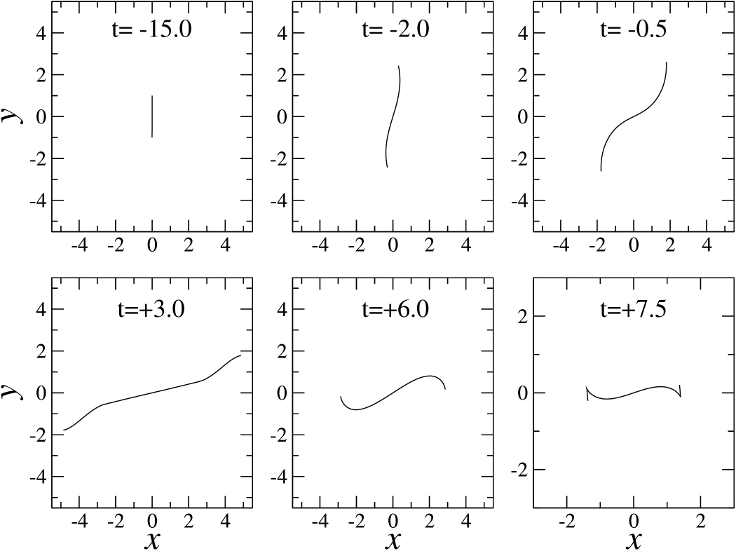
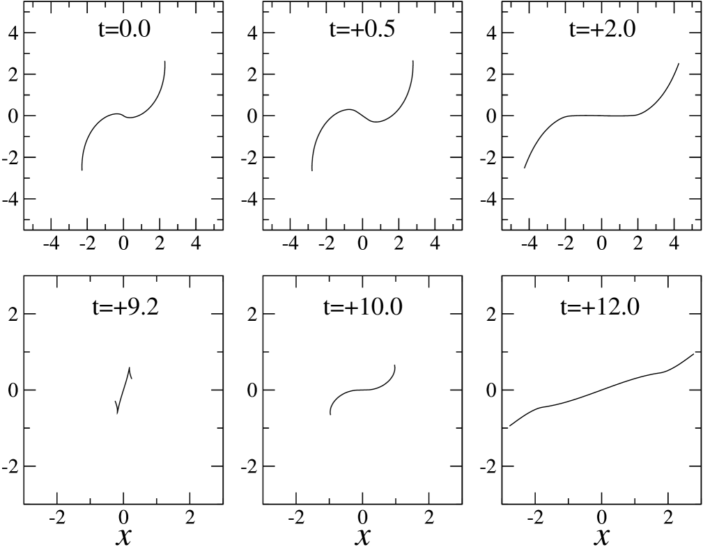
Figure 8: An incoming flat space-time rotor solution (23), with a small initial center of mass velocity, $v_{z}=0.01$ and $t_{s}=25$. The rotor evolves into an “S” shape in the $XY$ plane as the two opposite arms speed up towards the speed of light. The outgoing state involves a superposition of higher oscillation modes of the string, as may be seen from its evolution.

IV Rotor

The classical analogue of the graviton is a rotor solution, a spinning doubled line whose ends move at the speed of light. The flat space-time solution representing this incoming state is given by equation (23) or, if it has nonzero center of mass velocity, a Lorentz-boosted version of it. The appropriate initial conditions for the time-dependent background we study are given by computing the flat space-time left and right movers, and translating these into expanding universe left and right movers at the initial time. The solutions take the form of a doubled line for all time and the two end-points always move at the speed of light. The evolution is more complicated than that for a circular loop because there is a non-trivial dependence on $\sigma$.

There is a set of measure zero on the space of initial conditions where the evolution is singular, when the center of mass momentum of the rotor is precisely zero. Since there is no preferred direction orthogonal to the plane of the rotor, its central point must remain at rest for all $t$. This conflicts with the requirement that all points must move at the speed of light at $t=0$, hence the solution must go singular. However, we do not believe this will cause any problem in the quantum theory. States of zero momentum are of zero measure on phase space. So we shall study the behavior of a rotor with nonzero center of mass momentum $p_{z}$, in the limit as $p_{z}$ tends to zero. We shall find that the resulting non-analyticity in the classical solution is rather mild, and thus likely to overwhelmed by the measure in any physically realistic calculation.

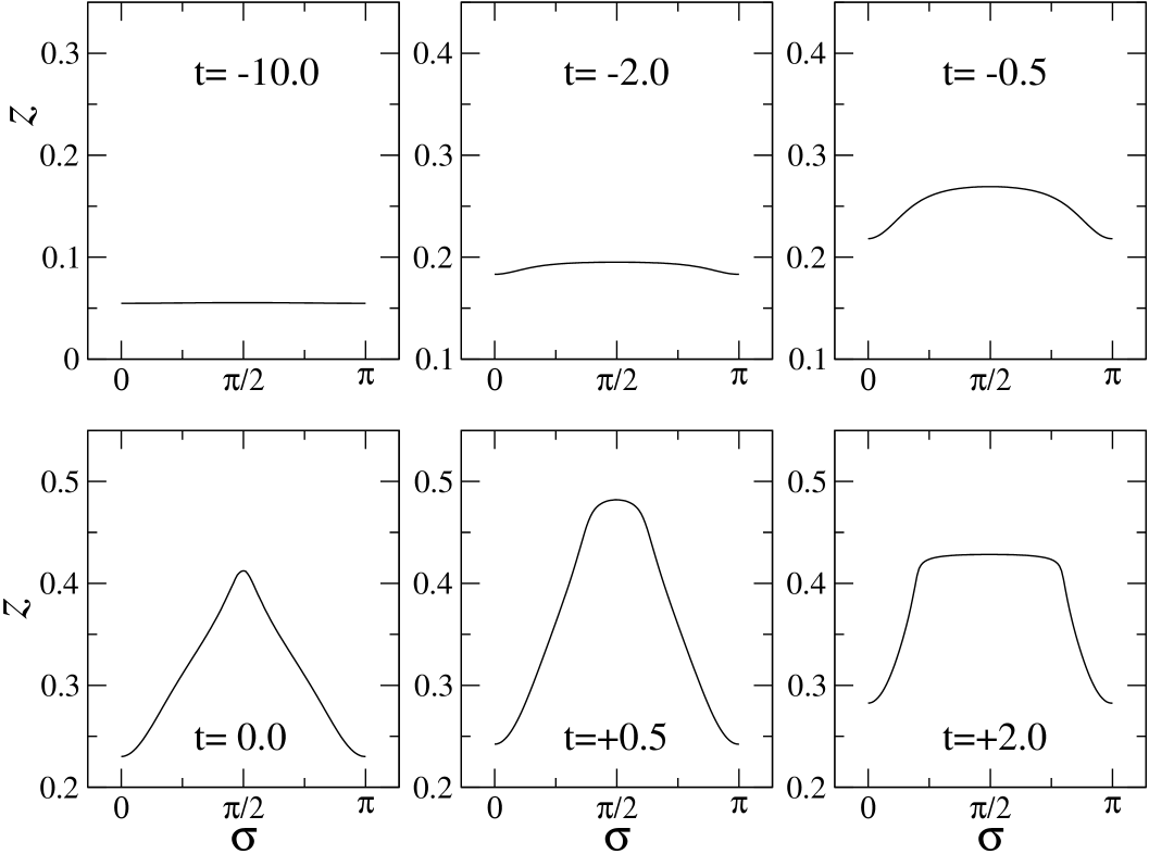
Figure 9: The profile of the incoming rotor shown in Figure 8, in the $z$ direction. The passage through $t=0$ results in a kink being produced at $t=0$, which then propagates outwards across the string.

By boosting the static solution (23) we can obtain a solution with arbitrary $v_{z}$, as defined in (25). Any simulation is then characterized by the starting time $t_{s}$ and the initial center of mass velocity $v_{z}$. Contrary to the circular loop, the oscillation phase of the incoming rotor is of no physical significance since it can be removed by a spatial rotation. Therefore, as far as the classical dynamics is concerned, the solution for a rotor depends only upon $v_{z}$ and there are no other parameters to consider.

The evolution of such a moving rotor across $t=0$ is illustrated in Figures 8 and 9. In the $XY$ plane, it develops an ‘S’ shape. This may be understood as a consequence of the opposite arms of the rotor speeding up to the speed of light in opposite directions as $t=0$ approaches. In the $Z$-direction, as the central point speeds up to the speed of light it creates a kink which then runs out across the string.

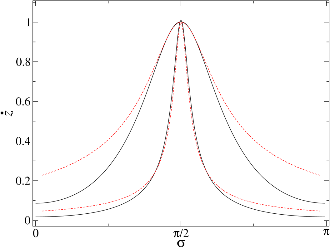
Figure 10: The kink in the transverse velocity $\dot{z}$ around the middle of the rotor, for two very small velocities. The profile (41) fits the shape very well for small transverse velocities (red dashed line), where the quantity $<\dot{z}_{0}>\equiv\int\epsilon_{0}\dot{z}_{0}d\sigma/\int\epsilon_{0}d\sigma$ measures the center of mass velocity at $t=0$ in the $z$ direction. The initial conditions were: $t_{s}=5$, $v_{z}=0.05$ for the wider curve and $v_{z}=0.01$ for the narrower curve.

IV.1 Profile of the Kink

As the rotor approaches $t=0$, it develops a kink in the direction of its motion, whose size and shape depends on the magnitude of the transverse momentum. For zero transverse momentum, the classical evolution is ill-defined. This is a set of measure zero, but the breakdown of the classical equations at $p_{z}=0$ may be indicative of some divergence. Therefore it is important to study the evolution for small $p_{z}$ to see whether physical quantities diverge that limit.

As the transverse momentum gets smaller, the kink gets narrower and narrower, as shown in Figure 10.

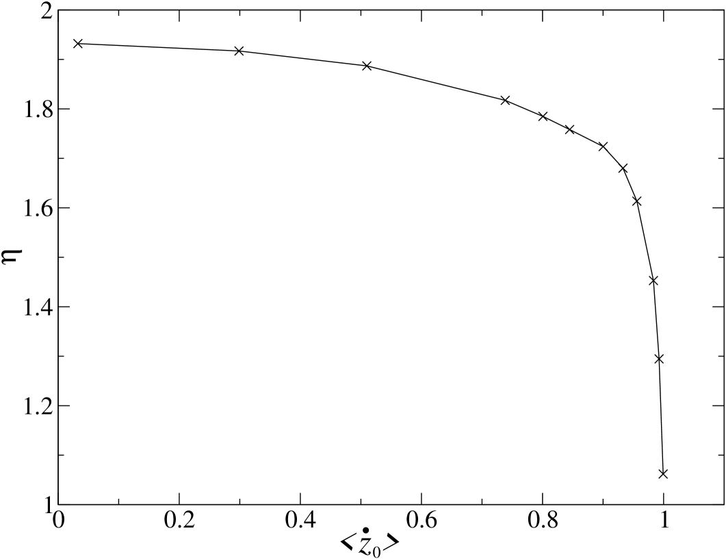
Figure 11: The energy ratio $\eta=E_{out}/E_{in}$ for a rotor is plotted against the average center of mass speed of the loop at $t=0$, i.e., $<\dot{z}_{0}>\equiv\int\epsilon_{0}\dot{z}_{0}d\sigma/\int\epsilon_{0}d\sigma$, showing that the net energy production is unaffected by the non-analytic spike produced in the limit of small transverse momentum.

The profile of the kink may be modeled analytically as follows. Consider the equation for the velocity of the string in the $z$ direction, $\dot{z}$. From equation (10), at $t=0$ we have

$$\dot{z}=\frac{\pi_{z}(0)}{\epsilon(0)}=\frac{\pi_{z}(0)}{\sqrt{\vec{\pi}\,(0)^{2}}},$$ (40)

where $\vec{\pi}=\epsilon\dot{\vec{x}}$ is the canonical momentum density at each point on the string, and we used (11) to get the last equality. For small transverse velocities, near the center of the rotor we can replace $\pi_{z}\sim<\dot{z}_{0}>\equiv\int\epsilon_{0}\dot{z}_{0}d\sigma/\int\epsilon_{0}d\sigma$ and use the Taylor expansion $\pi_{x}^{2}+\pi_{y}^{2}\sim(C\,\sigma)^{2}$, with $C$ a constant. Therefore, near the center of the rotor, the kink’s profile at $t=0$ is approximated by

$$\dot{z}=\frac{1}{\sqrt{1+\left(\frac{C\,\sigma}{<\dot{z}_{0}>}\right)^{2}}}.$$ (41)

This fit works well against our numerical results, as shown in Figure 10, with $C^{2}\sim 0.2$. As we take the centre of mass momentum of the loop to zero, the kink becomes more and more strongly localized and involves higher and higher oscillation modes of the string. However, these do not contribute significantly to the energy. Figure 11 shows $\eta=E_{out}/E_{in}$ as a function of the loop momentum. In the limit of small momentum, $\eta$ tends to a finite constant $\sim 1.93$, showing that there is little energy associated with the spike generated at the center of the rotor. We conclude that at low momenta, we produce a a non-differentiable but finite spike, although physical quantities like the energy or momentum remain perfectly finite.

IV.2 Expansion in the String Tension

Just as we have done for the circular loop, we can describe more general string states, including the rotor, using a formal expansion in the string tension. The details are given in Appendix A. Following the same general method as given for the circular loop, the zeroth order solution is given as

$$\vec{x}=\vec{x}_{0}+\frac{\vec{p}_{0}}{|\vec{x}^{\prime}_{0}|}\,\mathrm{sinh}^{-1}\bigg{(}\frac{|\vec{x}^{\prime}_{0}|}{|\vec{p}_{0}|}t\bigg{)},$$ (42)

where $\vec{p}_{0}$, $\vec{x}_{0}$ and $\vec{x}^{\prime}_{0}$ are functions of $\sigma$.

Higher terms in the expansion are more difficult to calculate and the integrals can only be done numerically (see Appendix A for details). Figure 12 shows the numerical solution plotted against the zeroth order term in the expansion, the first order term, and the flat space approximation, respectively. The comparison is made for an end point of the rotor (right plot) and a representative point further in (left plot). For the former, the adiabatic approximation holds very accurately up to Hubble crossing. Since the point is moving at the speed of light, the zeroth and first order terms of the expansion are nearly identical, providing a good approximation to the motion outside the Hubble radius. At Hubble re-entry, the solution reverts to a form close to flat-space evolution but this is more complex to determine hence we have not attempted to graph it. For generic points on the rotor, the adiabatic approximation is less accurate at earlier times: the speeding up of the central point as the kink is created in effect extracts energy from the normal spinning motion. As can be seen from the diagram, the first order expansion in the string tension does reasonably well in modeling the behavior around $t=0$ up to the first turning point.

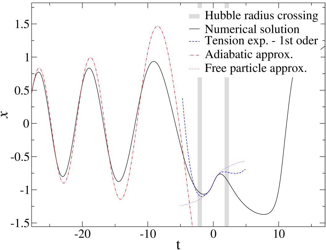
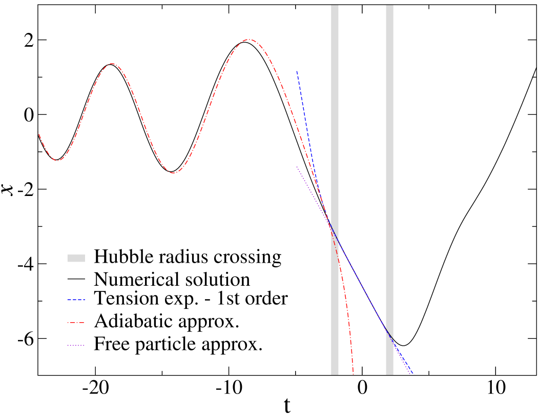
Figure 12: The numerical solution for two points on a rotor. The left plot shows the $x$ coordinate at $\sigma=\pi/4$ and the right plot shows the $x$ coordinate of the end point $\sigma=0$. The adiabatic flat space approximation reproduces the numerical solution reasonably well until the loop crosses the Hubble radius. Beyond this point, an expansion in the string tension becomes a much better description. In this plot, the initial center of mass speed was $v_{z}=0.05$ and $t_{s}$ was taken as $35$.

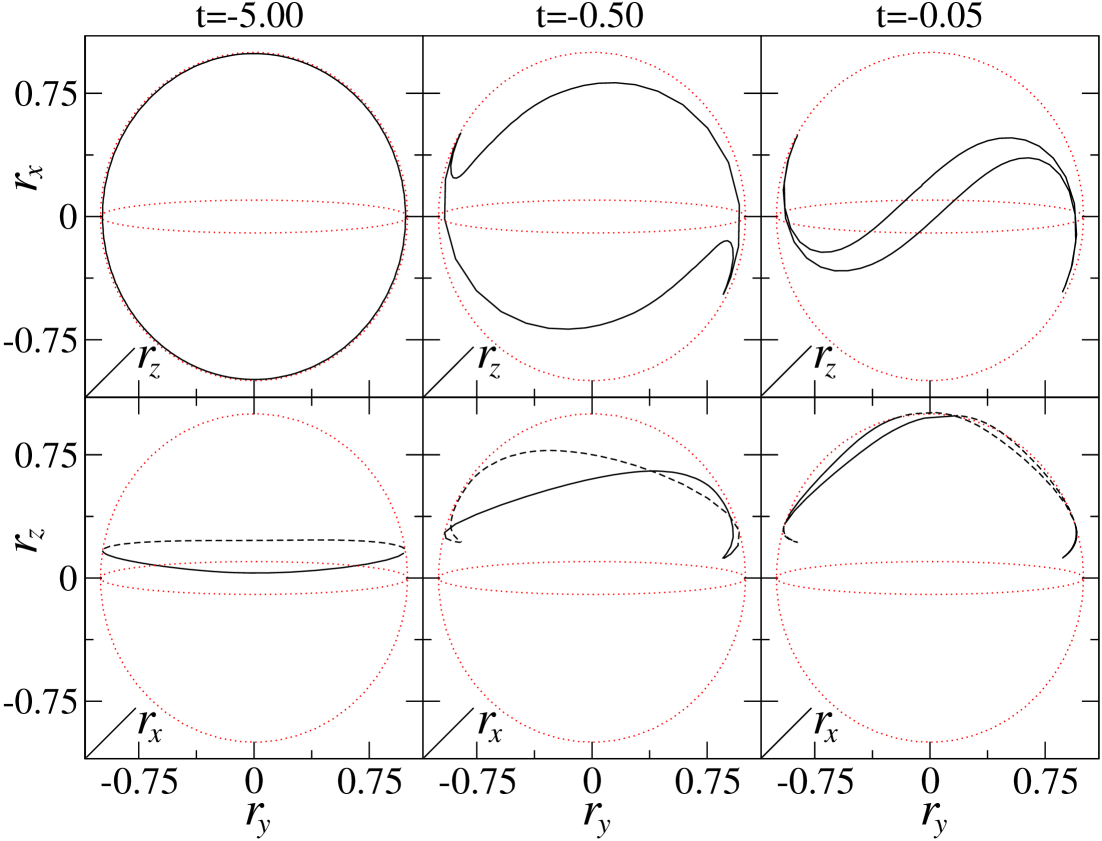
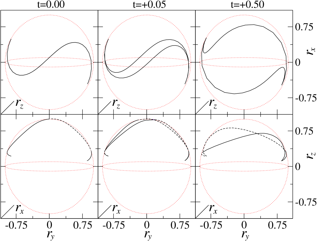
Figure 13: The evolution of the left mover $\vec{l}$ for an incoming rotor. The left mover defines a closed curve on a three-sphere. The right mover follows the same curve but with the opposite orientation. The condition (15) that the left and right movers coincide $t=0$, means that the evolution must deform the trajectories over the north pole of the three sphere. The only way to get the two curves to coincide is by deforming them into a double line at $t=0$, running directly through the north pole (or the south pole if $v_{z}$ is negative). The initial parameters here were $v_{z}=0.05$, $t_{s}=45$.

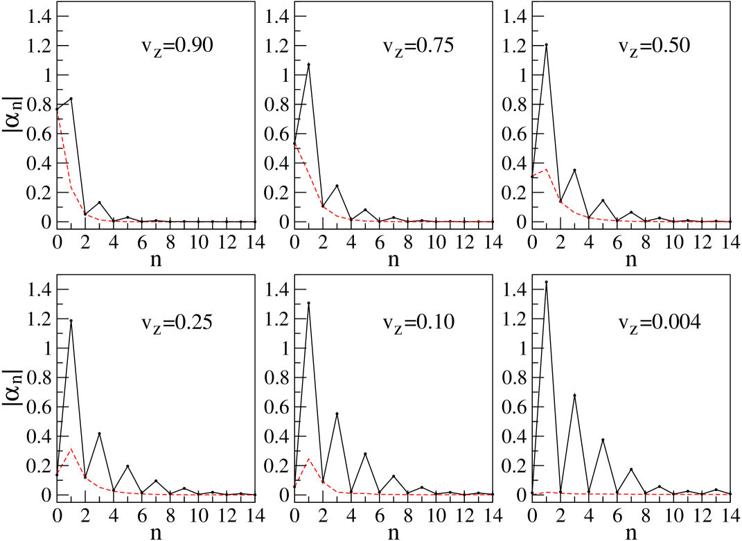
Figure 14: Fourier amplitudes of outgoing right movers calculated in the asymptotic adiabatic regime for different initial transverse speeds. The red dashed line shows the $z$ component only, hence $\alpha^{z}_{0}$ (the $n=0$ value of the red dashed line) is the final speed $v_{z}$. By symmetry, $\alpha^{x}$ and $\alpha^{y}$ have only odd-$n$ modes whereas $\alpha^{z}$ has both odd and even $n$ components. In these plots $t_{s}=25$.

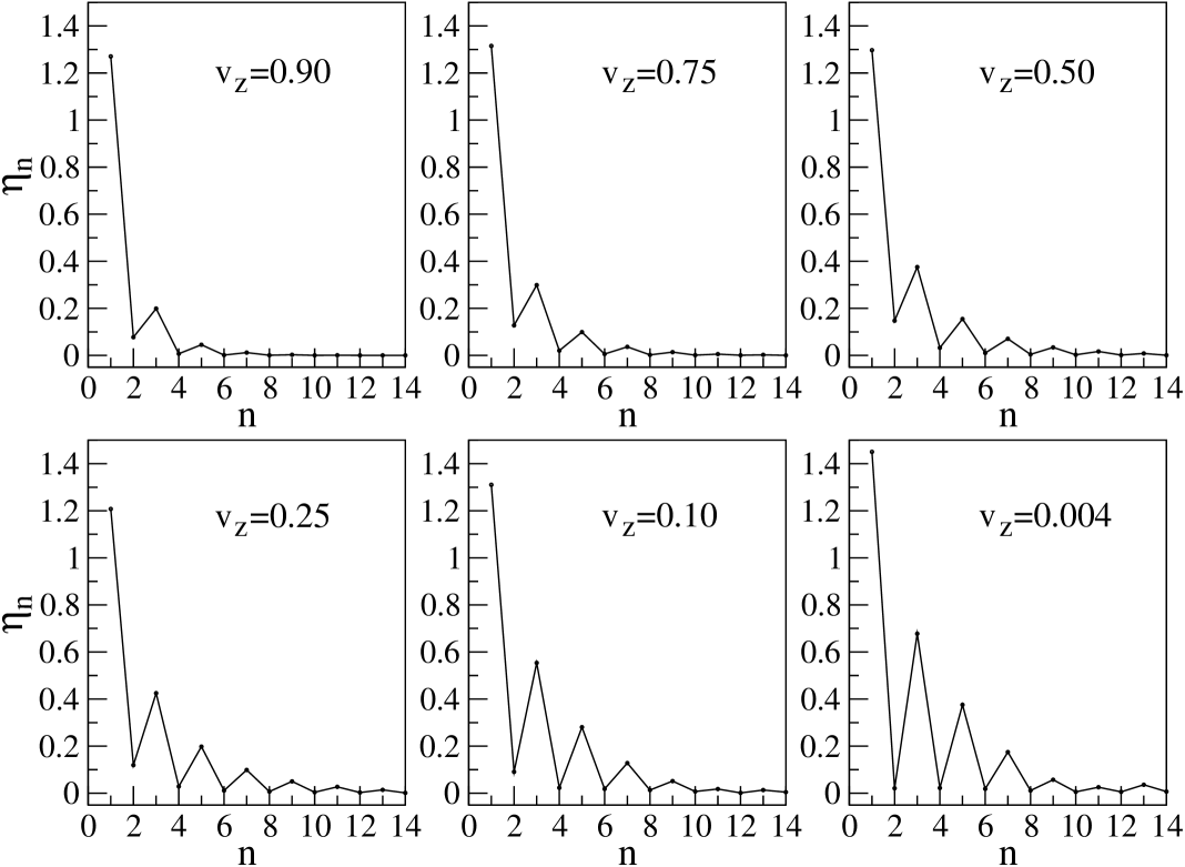
Figure 15: The energy ratio $\eta$ for each mode number $n$, representing the amplitude of each outgoing mode divided by the amplitude of the incoming mode. Larger initial speeds $v_{z}$ generate smaller amplitudes in the higher modes. The decay of $\eta$ with $n$ resembles the plane wave estimate ($\sim e^{-\beta\sqrt{n}}/\sqrt{n}$) found in  tolley for high velocities, but at low velocities $\eta$ decays more rapidly than expected from that work, and in particular the production of high $n$ modes remains finite.

IV.3 Outgoing state

When the rotor is evolved forward to large times, the outgoing state consists of a complicated mixture of higher oscillation modes. The precise mixture is most easily understood by representing the outgoing solution in left and right moving modes, which tend to fixed curves on the unit sphere at late times. One can also use the right and left movers to understand the motion of the rotor across the singularity (Figure 13). The two curves start out near the equator (for small $v_{z}$) and oppositely oriented. For zero center of mass velocity, the the curves are confined to the $xy$ plane and there is no way for them to coincide at $t=0$. However, if $v_{z}$ is positive (or negative), the curves sweep over the north (or south) pole and coincide at $t=0$.

To quantify the level of excitation produced in the passage across $t=0$, we can track the the evolution of the right and left movers in time at one particular value of $\sigma$ on the string. For very large times, the right and left movers look like flat space solutions and become periodic functions of proper time. Once the loop is well inside the Hubble radius, for a single period the difference between conformal time and proper time is negligible. Hence we can just choose one value of $\sigma$ and follow the evolution of left and right movers there. We write the expansion of the left and right movers (21) as

$$r^{i}=\sum_{n=-\infty}^{+\infty}\alpha^{i}_{n}e^{-in(t-\sigma)},\qquad\qquad l^{i}=\sum_{n=-\infty}^{+\infty}\tilde{\alpha}^{i}_{n}e^{-in(t+\sigma)},$$ (43)

and compute the $\alpha^{i}_{n}$ and $\tilde{\alpha}^{i}_{n}$ by Fourier transforming the solution with respect to $t$ over a single period. As is seen in Figure 19, identifying the periodicity is straightforward. As the initial center of mass velocity $v_{z}$ is tuned down, modes at higher and higher $n$ are excited, although as shown above, the total energy in the outgoing string converges to a finite limit as $v_{z}$ tends to zero.

 

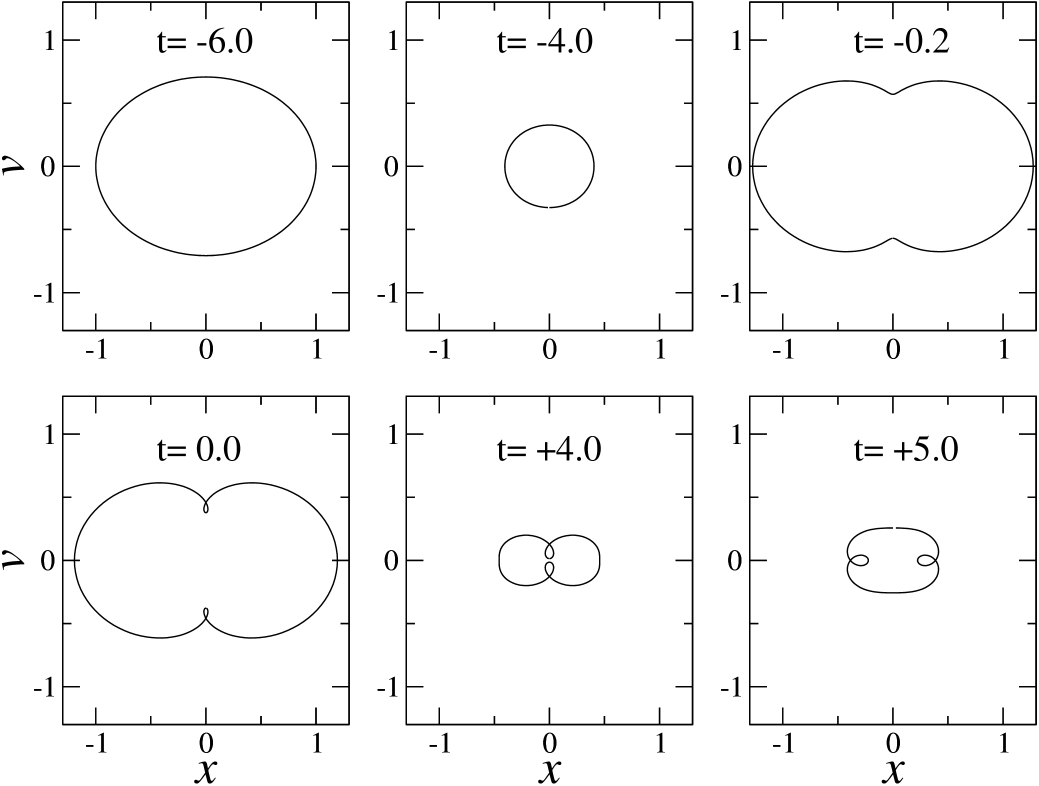
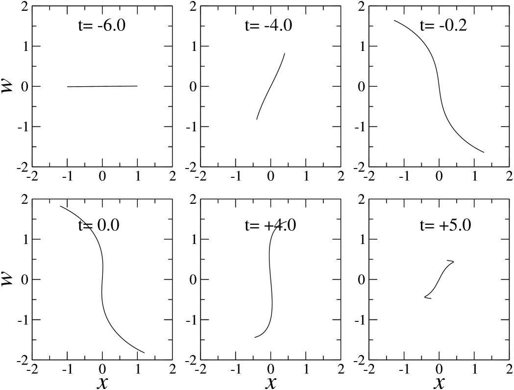
Figure 16: Evolution of the classical analog of the antisymmetric tensor (24) across the singularity. The six plots on the left show the behavior in the $xv$ plane, where, inside the Hubble radius, the solution is an oscillating elliptical loop. Higher modes are excited as $t=0$ is crossed. The plots on the left show the projection into the $xw$ plane, in which the solution always appears as a doubled line. Again, it is clear from the pictures that higher modes have been excited. For this case, $t_{s}=6$ was used.

V Classical analog of the Antisymmetric Tensor

To complete our discussion of low mode solutions, we consider configurations with intermediate angular momentum, which are the analog of the massless antisymmetric tensor states of the quantized string. The corresponding flat-space solution was given in (24), and its evolution, illustrated in Figure 2, consists of a spinning state whose shape alternates between an ellipse and a doubled line. The motion is simplest when projected onto planes spanned by the vectors: $\hat{x}=(1,0,...,0)$, $\hat{v}=\frac{1}{\sqrt{2}}(0,1,1,0,...,0)$ and $\hat{w}=\frac{1}{\sqrt{2}}(0,-1,1,0,...,0)$. In the $xv$ plane the solution appears as an ellipse which shrinks to a point and re-expands. In the $xw$ plane the motion is similar to that of the rotor, but the length of the rotor oscillates. (see Figure 2).

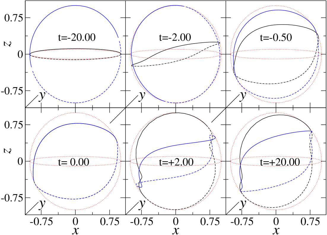
Figure 17: An incoming classical analog of the antisymmetric tensor state is represented by left movers (blue lines) and right movers (black lines) on the sphere. At $t=0$ the left and right movers coincide in a doubled line.

If we follow the evolution of such a solution towards $t=0$, once it has crossed the Hubble horizon, it practically freezes in size in the $x$ and $w$ axes, and either its position or its momentum freeze in the $v$ coordinate. Apart from the special case where the elliptical motion has a maximum at $t=0$ (which is mildly non-analytic, like the case of a circular loop), the motion is regular across $t=0$ and produces a tower of higher excited modes (see Figure 16). If the position is the frozen variable in the $v$ direction, there are fewer excited modes produced, and conversely if the momentum is the frozen variable. As for the rotor, we can picture the evolution of the antisymmetric tensor’s classical analog in terms of left and right movers on the sphere (Figure 17).

VI Quantum evolution across t=0

In this section we treat the quantum production of excited string modes in a simple approximation, which may be extended to discuss more complicated string states. As we have already indicated, for large string states it is reasonable to expect that, provided the quantum theory remains well-defined, quantum corrections should be small and our classical calculations should be accurate.

Here we shall limit ourselves to an illustrative example, consisting of a truncation of the full theory to the simplest oscillation mode, namely a circular loop. The method we use generalizes to more interesting excited states and we shall study this in future work. We start from the classical equations of motion for a loop,

$${dp\over dt}=-{t^{2}\,\rho\over H},\qquad{d\rho\over dt}={p\over H},\qquad H^{2}=p^{2}+t^{2}\rho^{2}.$$ (44)

We would like to quantize these equations, but the nonlinearity renders this difficult. We proceed in the following approximation. The operator $\hat{H}^{2}=\hat{p}^{2}+t^{2}\hat{\rho}^{2}$ is positive definite, and so it is not unreasonable to attempt to approximate the terms $H$ in the first two equations with the $c$-number quantity,

$$H_{c}(t)\equiv\sqrt{\langle\hat{H}^{2}(t)\rangle}.$$ (45)

With this replacement, we have only to solve the linear quantum system whose Heisenberg equations of motion are

$${d\hat{p}\over dt}=-{t^{2}\,\hat{\rho}\over H_{c}(t)},\qquad{d\hat{\rho}\over dt}={\hat{p}\over H_{c}(t)},$$ (46)

where $H_{c}(t)$ is as yet undetermined.

The general solution to (44) may be expressed in terms of two linearly independent solutions, defined at some initial time $t_{0}$, as follows:

$$\hat{\rho}(t) = \hat{\rho}_{0}f_{\rho}(t,t_{0})+\hat{p}_{0}g_{\rho}(t,t_{0}),$$ (47)

$$\hat{p}(t) = \hat{\rho}_{0}f_{p}(t,t_{0})+\hat{p}_{0}g_{p}(t,t_{0}),$$ (48)

where $f_{\rho}$, $f_{p}$, $g_{\rho}$ and $g_{p}$ satisfy the initial conditions $f_{\rho}=1$, $f_{p}=0$, $g_{\rho}=0$ and $g_{p}=1$ at time $t=t_{0}$.

We now wish to express the operators $\hat{\rho}_{0}$ and $\hat{p}_{0}$ in terms of creation and annihilation operators for the incoming vacuum state. To do so, we need to identify the relation between $\rho$ and $p$ and the properly normalized coordinate and momentum of a harmonic oscillator at large $|t|$. Noticing that the quantity as

$$\hat{\mathcal{P}}={\hat{H}^{2}\over 2|t|}={\hat{p}^{2}+t^{2}\hat{\rho}^{2}\over 2|t|},$$ (49)

defined in (32), is an action variable at large $|t|$ (see Section III.1), we identify the proper momentum $\hat{\pi}=\hat{p}/\sqrt{|t|}$ and radius $\hat{R}=\hat{\rho}\sqrt{|t|}$ as the asymptotic coordinate and momentum of a corresponding harmonic oscillator. These variables can then be expressed in terms of creation and annihilation operators, defined at some large negative time $t_{0}$:

$$\hat{\rho}_{0}={(a_{0}+a_{0}^{\dagger})\over\sqrt{2|t_{0}|}},\qquad\hat{p}_{0}=\sqrt{|t_{0}|\over 2}{(a_{0}-a_{0}^{\dagger})\over i}.$$ (50)

It is then clear how to compute the function $H_{c}(t)$, from the formulae above, for any chosen incoming state. In particular, in the incoming vacuum state defined by $a_{0}|0\rangle_{in}=0$, we find

$$H_{c}^{2}(t)={1\over 2}\left({f_{p}^{2}\over|t_{0}|}+|t_{0}|g_{p}^{2}+t^{2}\left({f_{\rho}^{2}\over|t_{0}|}+|t_{0}|g_{\rho}^{2}\right)\right).$$ (51)

It is straightforward to solve equations (46) for the two independent solutions $f$ and $g$, using (51) to define $H_{c}(t)$. This then provides a self-consistent semi-classical approximation to the full quantum evolution.

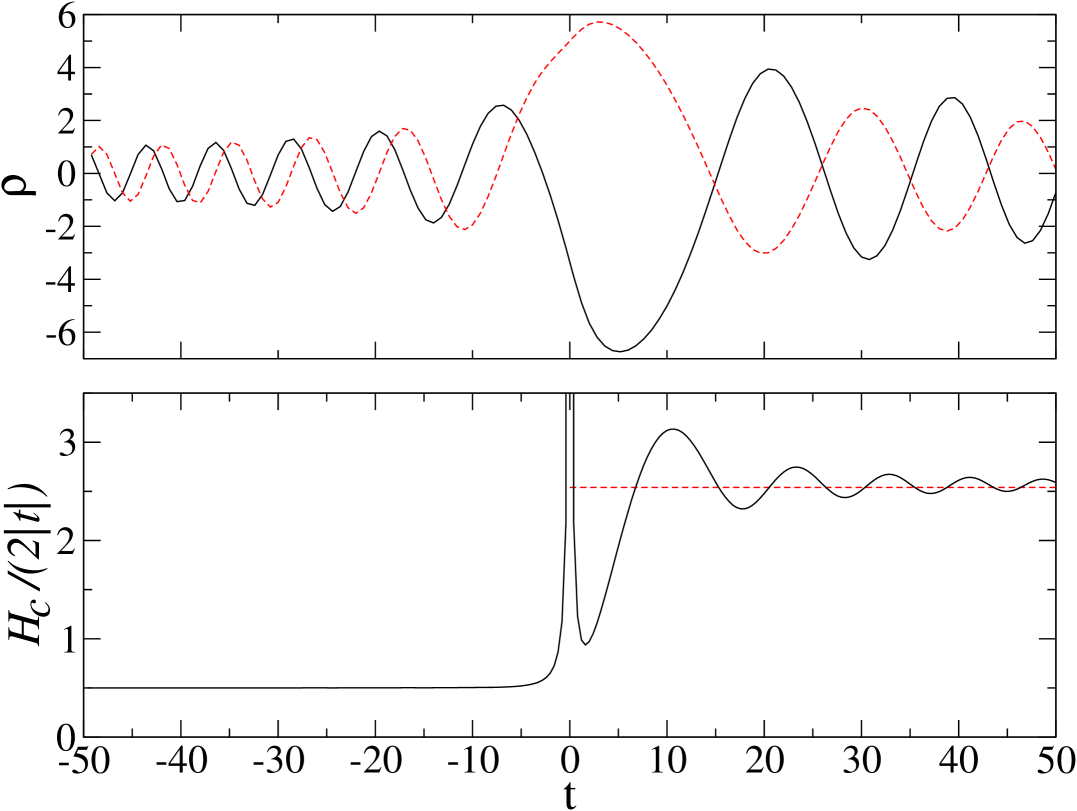
Figure 18: The quantum creation of higher excitations on a circular loop, sent in in its ground state. The upper plot shows the two independent solutions $f_{\rho}$ and $g_{\rho}$ defined in the text. The lower plot shows the evolution of the ‘energy’ $H_{c}/(2|t|)$. This is not well-defined at $t=0$, even though the equations of motion are regular there. For a loop sent in in its vacuum state, with an energy ${1\over 2}$ in these units, the outgoing state has an energy of approximately $2.54$. The increase in energy is due to quantum mode creation as the loop crosses $t=0$.

Figure 18 shows the results of this calculation, for the incoming vacuum state. From formula (49), we identify $H_{c}^{2}/(2|t|)$ as the asymptotic harmonic oscillator energy at late times, which may in our chosen units be expressed as $\,{}_{in}\langle 0|(N_{out}+{1\over 2})|0\rangle_{in}$ where $N$ is the usual number operator. Therefore, from the Figure, we see that in the outgoing state,

$${}_{in}\langle 0|N_{out}|0\rangle_{in}=|\beta|^{2}\approx 2.04,$$ (52)

where $\beta$ is the usual Bogoliubov coefficient measuring the amount of particle creation birrell . Similar results are obtained for excited incoming states. One can straightforwardly compute the Bogoliubov coefficients $\alpha$ and $\beta$ including their phases, using the same method. The results will be given elsewhere.

VII Summary

We have herein discussed how classical strings propagate through the simplest possible big crunch/big bang transition in M theory, and made a start on considering the quantum problem. As we have discussed, the usual $\alpha^{\prime}$ expansion must be replaced by an expansion in the string tension, i.e. $1/\alpha^{\prime}$, once the Hubble radius falls below the string length. We have presented an analytic solution of the Nambu equations as a formal expansion in the string tension, which could form the basis for a quantum treatment of the small time regime.

Using the decomposition into right and left movers, we have shown how higher oscillation modes are excited by a finite amount as the string crosses singularity. We have also given a discussion of some special cases where the string is constrained by symmetry to be static at $t=0$. Except for a set of configurations of measure zero, the classical counterparts of the dilaton, graviton and antisymmetric tensor string states evolve smoothly across $t=0$.

We have made a modest start at describing the quantum evolution of string across $t=0$, discussing a truncation of the theory to the lowest mode describing a circular loop. The method we have employed appears to be readily extendible to more complex incoming states, and to the inclusion of more and more string modes. As this is done, we can begin to address the subtle issues of renormalization which we have so far ignored. It may also be feasible to go beyond the first semiclassical calculation we have described.

Our main conclusion is that classical strings pass smoothly through singularities of the simple type studied here, and the excitations they acquire in doing so may be readily calculated in a formal expansion in the string tension. While much remains to be done to develop a full quantum description, our findings reported here are encouraging.

Acknowledgements

We thank Malcolm Perry, Paul Steinhardt and Andrew Tolley for discussions. This work was supported by CONACYT, SEP and the Cambridge Overseas Trust (GN) and PPARC (NT). NT is the Darley Professorial Fellow at Cambridge.

Appendix A Series expansion around $t=0$

A.1 Circular loop

As explained in Section III.3, in order to study the motion of the string across $t=0$ we perform a formal expansion in the string tension. We do so by introducing a formal parameter $\lambda$ in front of the relevant term in the Hamiltonian, and then we solve the equations of motion to a given order in $\lambda$. Finally, we take $\lambda=1$. With this parameter $\lambda$, equations (29)-(31) take the form (38), which we repeat here:

$${dp\over dt}=-\lambda{t^{2}\,\rho\over H},\qquad{d\rho\over dt}={p\over H},\qquad{dH^{2}\over dt}={2\over t}(H^{2}-p^{2}).$$ (53)

From this point, there is only one consistent way to proceed. At lowest order in $\lambda$, we solve the above equations with $\lambda=0$. Then we substitute this solution into the term involving $\lambda$ and integrate with respect to $t$ to obtain first $p$, then $H$ and finally $\rho$ to order $\lambda$. This solution is again substituted into the right hand side of the first equation, and the procedure continued. Effectively, we have

$${dp^{(n)}\over dt}=-\lambda{t^{2}\left(\rho\over H\right)^{(n-1)}},\qquad{d(t^{-2}(H^{2})^{(n)})\over dt}=-2\frac{(p^{2})^{(n)}}{t^{3}},$$ (54)

which can be written as integral equations,

$$p^{(n)}=p_{0}+\lambda I^{(n-1)},\qquad(H^{2})^{(n)}=p^{2}_{0}+\rho_{0}^{2}t^{2}-4\lambda p_{0}J^{(n-1)}-2\lambda^{2}K^{(n-2)},$$ (55)

where $p(0)=p_{0}$, $\rho(0)=\rho_{0}$ and $I^{(n)}(t),$ $J(^{(n)}t),$ and $K^{(n)}(t)$ are defined as

$$I^{(n)}(t)=-\int_{0}^{t}{\tilde{t}^{2}\left(\!\rho(\tilde{t})\over H(\tilde{t})\!\right)^{(n)}}d\tilde{t}, \qquad J^{(n)}(t)=\int_{0}^{t}\frac{I^{(n)}(\tilde{t})}{{\tilde{t}}^{3}}d\tilde{t},$$ (56)

$$K^{(n)}(t)=\int_{0}^{t} \frac{\left([I(\tilde{t})]^{2}\right)^{(n)}}{{\tilde{t}}^{3}}d\tilde{t},$$ (57)

Now equations (55) have the desired form. Finally, we use these solutions for $p$ and $H$ to construct $\rho$ to the same order in $\lambda$ by expanding the quotient

$${d\rho^{(n)}\over dt}=\left(\frac{p}{H}\right)^{(n)}.$$ (58)

To zeroth order in $\lambda$, we find

$$p^{(0)}=p_{0},\qquad\qquad H^{(0)}=\sqrt{p^{2}_{0}+C^{2}t^{2}},$$ (59)

where $C$ is an integration constant that we will fix at the end, after setting $\lambda=1$. The solution to $\rho^{(0)}$ is then given by

$$\rho^{(0)}=\rho_{0}+\frac{p_{0}}{|C|}\sinh^{-1}\left(\frac{|C|}{|p_{0}|}t\right).$$ (60)

In order to construct the next order solutions, there is a change of variables which simplifies the expressions, given by

$$\chi\equiv\sinh^{-1}\left(\frac{|C|}{|p_{0}|}t\right),$$ (61)

thus the zeroth order solutions look like

$$p^{(0)}=p_{0},\qquad\qquad H^{(0)}=p_{0}\cosh(\chi),\qquad\qquad\rho^{(0)}=\rho_{0}+\frac{p_{0}}{|C|}\chi.$$ (62)

To next order in $\lambda$, we get

$$p^{(1)} = p_{0}\Bigg{[}1+\lambda\frac{p_{0}\,\rho_{0}}{4{C}^{2}}\left(2\chi-\sinh(2\chi)\right)+\lambda\frac{p_{0}^{2}}{4{C}^{4}}\left({\chi}^{2}+\sinh^{2}(\chi)-\chi\sinh(2\chi)\right)\Bigg{]},$$

$$(H^{2})^{(1)} = p_{0}^{2}\Bigg{[}\cosh^{2}(\chi)+\lambda\frac{p_{0}\,\rho_{0}}{2|C|^{3}}(2\chi\cosh(2\chi)-\sinh(2\chi))$$ (63)

$$\hskip 28.45274pt+\lambda\frac{p^{2}_{0}}{2C^{4}}\Big{(}\chi^{2}\cosh(2\chi)+\sinh^{2}(\chi)-\chi\sinh(2\chi)\Big{)}\Bigg{]}.$$

The parameter $\lambda$ governs the dynamics of solutions near $t=0$, so it can not appear in the initial conditions. Consequently, after setting $\lambda=1$ the value for $C$ is determined using the equation for the Hamiltonian (29), which implies ${H}^{\prime\prime}(0)=2\rho_{0}^{2}$. From the solution of $(H^{2})^{(0)}$, or equivalently $(H^{2})^{(1)}$, at $t=0$ one reads $C=\rho_{0}$. Therefore, the solutions for $p^{(1)}$ and $H^{(1)}$ are just polynomials in the scale-invariant parameter $|p_{0}/\rho_{0}^{2}|$.

Note that the functions $p^{(1)}$ has an odd and an even piece with respect to $\chi$. Therefore, the function will be more symmetric around $t=0$ if $|p_{0}/\rho_{0}^{2}|\gg 1$, and more asymmetric for the converse value. The odd-$\chi$ part will always have a zero near $t=0$, which represents either the maximum or the minimum in $\rho$ near $t=0$. The other zero of $p$ depends on the even-$\chi$ piece, which is close to $t=0$ only for $|p_{0}/\rho_{0}^{2}|\gg 1$. However, the series is only accurate for small $\chi$ which guarantees $-t^{2}\rho/H$ is small after taking $\lambda=1$, so only if the invariant parameter $|p_{0}/\rho_{0}^{2}|\ll 1$ one can go a little beyond the Hubble radius crossing.

By expanding the quotient on the RHS of equation (58) to first order in $\lambda$ we obtain $\rho^{(1)}$, which looks like

$$\rho^{(1)} = \rho_{0}\Bigg{[}1+\frac{p_{0}}{\rho_{0}\,|C|}\chi+\lambda\frac{p_{0}^{2}}{4C_{0}^{4}}\left(\chi(2\tanh(\chi)-\chi)-\sinh^{2}(\chi)\right)$$

$$\hskip 19.91684pt-\lambda\frac{p_{0}^{3}}{12\,\rho_{0}\,|C|^{5}}\left(9\chi+2\chi^{3}+3\chi\cosh(2\chi)-3\sinh(2\chi)-6\tanh(\chi)-6\chi^{2}\tanh(\chi)\right)\Bigg{]}.$$

Again, $\rho^{(1)}$ has piece which is an even function of $\chi$, but now there are two terms which are odd-$\chi$ functions. It is due to this extra order term in $p_{0}/\rho_{0}^{2}$ that the $\rho$ solution is more symmetric if $|p_{0}/\rho_{0}^{2}|\ll 1$ and asymmetric if $|p_{0}/\rho_{0}^{2}|\gg 1$, in opposition to $p^{(1)}$.
In order to obtain better precision and more maxima and minima in $\rho$ with this series, one has to go beyond first order in $\lambda$. However, the integrals become harder and harder to solve. Just to illustrate the flavor of the next order solutions, $\rho^{(2)}$ is given by

$$\rho^{(2)} = \rho_{0}\cosh^{3}(\chi)\Bigg{\{}\cosh^{3}(\chi)+\frac{p_{0}}{\rho_{0}^{2}}\left[\chi\cosh^{3}(\chi)\right]$$

$$+\frac{p_{0}^{2}}{16\rho_{0}^{4}}\cosh^{2}(\chi)\bigg{[}(-1+4\chi^{2})\cosh(\chi)+\cosh(3\chi)-8\chi\sinh(\chi)\bigg{]}$$

$$-\frac{p_{0}^{3}}{768\rho_{o}^{6}}\bigg{[}32\cosh^{3}(\chi)\left({\pi}^{2}+12\chi^{2}-24\chi\ln(2\cosh(\chi)+12{\mathrm{Li}_{2}}(-e^{-2\,\chi}))\right)$$

$$\hskip 28.45274pt+\chi(9\cosh(\chi)-4\cosh(3\chi)-12\cosh(5\chi))+(24{\chi}^{2}-42)\sinh(\chi)$$

$$\hskip 28.45274pt+(120{\chi}^{2}-27)\sinh(3\chi)+15\sinh(5\chi)\bigg{]}$$

$$+\frac{{{p_{0}}}^{4}}{12288{{\rho_{0}}}^{7}}\bigg{[}3\left(347+208{\chi}^{2}\right)\cosh(5\chi)+3\cosh(7\chi)-1440\chi\sinh(5\chi)$$

$$\hskip 28.45274pt+128\cosh^{3}(\chi)\left(144\chi^{2}\ln(2)-96{\chi}^{3}+5{\chi}^{4}+48(1+3{\chi}^{2})\ln(\cosh(\chi))\right)$$

$$\hskip 28.45274pt+6\cosh(\chi)\left(-647-40{\chi}^{2}+(473+1248)\cosh(2\chi)\right)$$

$$\hskip 28.45274pt-96\chi\left(2(17+6{\chi}^{2})\sinh(\chi)+(65+28{\chi}^{2})\sinh(3\chi)\right)$$

$$\hskip 28.45274pt-96\left(24{\cosh(\chi)}^{3}\left(4{\mathrm{Li}_{3}}(-e^{-2\chi})+8{\mathrm{Li}_{2}}(-e^{-2\chi})+3{\zeta}(3)\right)\right)\bigg{]}$$

$$-\frac{p_{0}^{5}}{122880\rho_{0}^{9}}\bigg{[}4\cosh(\chi)\left(16\cosh^{2}(\chi)(40\pi^{2}+7\pi^{4}+480\chi^{2}+720\chi^{4}-20\chi^{6})\right)$$

$$\hskip 28.45274pt-320\chi^{3}\cosh(\chi)\left(-4+13\cosh(4\chi)+57\cosh(2\chi)+192\cosh^{2}(\chi)\ln(2\cosh(\chi))\right)$$

$$\hskip 28.45274pt+15360\cosh^{3}(\chi)\left((2+6\chi^{2})\mathrm{Li}_{2}(-e^{-2\chi})+6\chi\mathrm{Li}_{3}(-e^{-2\chi})+3\mathrm{Li}_{4}(-e^{-2\chi})\right)$$

$$\hskip 28.45274pt+30\sinh(\chi)\left(1204+1824\chi^{2}+320\chi^{4}+1845\cosh(2\chi)+2560\chi^{2}\cosh(2\chi)\right)$$

$$\hskip 28.45274pt+30\sinh(\chi)\left(448\chi^{4}\cosh(2\chi)+516\cosh(4\chi)+480\chi^{2}\cosh(4\chi)+3\cosh(6\chi)\right)\bigg{]}\Bigg{\}}$$

where we have already set $\lambda=1$ and $C=\rho_{0}$. In the above expression, $\zeta(x)$ is the Riemann Zeta function and $\mathrm{Li}_{n}(z)$ is the $n$-degree Polylogarithm function, which is defined as  mathworld

$$\mathrm{Li}_{n}(z)\equiv\sum_{k=1}^{\infty}\frac{z^{k}}{k^{n}},$$ (66)

where $z$ belongs to the open unit disk in the complex plane, and is defined uniquely for $|z|>1$ by analytic continuation.

A.2 Expansion in the string tension for a general string configuration

In this Appendix we want to construct a formal expansion in the string tension for an arbitrary string configuration. Our starting point is the Hamiltonian corresponding to the action (9),

$$H=\int d\sigma{\cal H},\qquad{\cal H}=\sqrt{{\cal P}^{2}+\lambda t^{2}(\vec{x}^{\prime})^{2}},$$ (67)

where in analogy with the circle, we have chosen to work in units where $\mu_{2}\theta_{0}=1$ but we have inserted a formal parameter $\lambda$ in front of the term involving the string tension. The Hamiltonian equations read as follows:

$${\partial_{t}{\cal P}}=\lambda t^{2}\partial_{\sigma}\left({\partial_{\sigma}\vec{x}\over{\cal H}}\right),\qquad\partial_{t}\vec{x}={{\cal P}\over{\cal H}},\qquad\partial_{t}{\cal H}^{2}={2\over t}\left({\cal H}^{2}-{\cal P}^{2}\right).$$ (68)

The second equation can be written in the integral form

$$\dot{\vec{x}}=\frac{\vec{p}_{0}+\lambda{\vec{I}}}{{\cal H}},$$ (69)

where $\vec{p}_{0}=\vec{p}_{0}(\sigma)$ is the momentum distribution at $t=0$, and

$$\vec{I}^{(n)}(t,\sigma)=\int_{0}^{t}d\tilde{t}\,\tilde{t}^{2}\partial_{\sigma}\left({\partial_{\sigma}\vec{x}(\tilde{t},\sigma)\over{\cal H}(\tilde{t},\sigma)}\right)^{(n)}$$ (70)

Similarly, ${\cal H}(t,\sigma)$ also has an expansion with respect to $\lambda$, given by

$$({\cal H}^{2})^{(n)}=\vec{p}_{0}^{\,2}+D^{2}_{0}t^{2}-4\lambda\vec{p}_{0}\cdot\vec{J}^{(n-1)}-2\lambda K^{(n-2)},$$ (71)

where $D_{0}^{2}$ is an integration constant that we will fix after taking $\lambda=1$, and

$$\vec{J}^{(n)}(t,\sigma)=\int_{0}^{t}\frac{d\tilde{t}}{\tilde{t}^{3}}\vec{I}^{(n)}(\tilde{t},\sigma),\qquad K^{(n)}(t,\sigma)=\int_{0}^{t}\frac{d\tilde{t}}{\tilde{t}^{3}}\left(\big{[}\vec{I}(\tilde{t},\sigma)\big{]}^{2}\right)^{(n)}$$ (72)

With these definitions, equation (69) becomes $\partial_{t}\vec{x}^{(n)}=\left({{\cal P}\over{\cal H}}\right)^{(n)}$, and hence the zeroth order equation in $\lambda$ is

$${\dot{\vec{x}}}^{(0)}=\frac{\vec{p}_{0}}{\sqrt{\vec{p}_{0}^{\,2}+D^{2}_{0}t^{2}}},$$ (73)

which is easily solved by

$$\vec{x}^{(0)}=\vec{x}_{0}+\frac{\vec{p}_{0}}{|D_{0}|}\,\mathrm{sinh}^{-1}\bigg{(}\frac{|D_{0}|}{|\vec{p}_{0}|}t\bigg{)},$$ (74)

where $\vec{x}_{0}$ is the string shape at $t=0$. After setting $\lambda=1$ the Hamiltonian equation 67 implies ${\cal H^{2}}^{\prime\prime}(0)=2(\vec{x}^{\prime}(0))^{2}$, which translates into $D_{0}=|\vec{x}^{\prime}(0)|$.

Now, to first order in $\lambda$, we find the equation for $\vec{x}$ is given by

$$\dot{\vec{x}}^{(1)}=\frac{\vec{p}_{0}}{\sqrt{\vec{p}_{0}^{\,2}+D_{0}^{2}t^{2}}}\bigg{[}1+\lambda I^{(0)}+\lambda\frac{2t^{2}\vec{p}_{0}\cdot\vec{J}^{(0)}}{\vec{p}_{0}^{\,2}+D_{0}^{2}t^{2}}\bigg{]},$$ (75)

and with a similar change of variables to that we introduced before for the circular loop, $\chi=\sinh^{-1}\left(\frac{|D_{0}|t}{|\vec{p}_{0}|}\right)$, the first order solution reduces to

$$\vec{x}=\vec{x}^{(0)}+\!\frac{\lambda}{|D_{0}|}\!\int_{0}^{\chi}\!d\vartheta\vec{I}^{(0)}(\vartheta,\sigma)+\frac{2\lambda\vec{p}_{0}}{|D_{0}|\vec{p}_{0}^{2}}\int_{0}^{\chi}\!\frac{\sinh^{2}(\vartheta)}{\cosh(\vartheta)}\int_{0}^{\vartheta}\frac{\cosh(\tilde{\vartheta})}{\sinh^{3}(\tilde{\vartheta})}\vec{p}_{0}\cdot\vec{I}^{(0)}(\tilde{\vartheta},\sigma)d\tilde{\vartheta}d\vartheta$$ (76)

These integrals can be reduced to a single integral by changing the order of the integrals, provided no convergence issues arise. For situations where the parameter $|\vec{p}_{0}|/\vec{x^{\prime}}_{0}|\sim 1$, there is no difficulty and the the integrals can be exchanged in the following way

$$\int_{0}^{\chi}d\vartheta\vec{I}^{(0)}(\vartheta,\sigma) = \frac{\vec{p}_{0}^{2}}{D_{0}^{2}}\int_{0}^{\chi}d\tilde{\vartheta}\sinh^{2}(\tilde{\vartheta})\cosh(\tilde{\vartheta})(\vartheta-\tilde{\vartheta})\partial_{\sigma}\left({\partial_{\sigma}\vec{x}(\tilde{\vartheta},\sigma)\over{\cal H}(\tilde{\vartheta},\sigma)}\right)^{(0)},$$

$$\int_{0}^{\vartheta}\frac{\cosh(\tilde{\vartheta})d\tilde{\vartheta}}{\sinh^{3}(\tilde{\vartheta})}\vec{I}^{(0)}(\tilde{\vartheta},\sigma) = \frac{\vec{p}_{0}^{2}}{2\,D_{0}^{2}}\int_{0}^{\vartheta}d\tilde{\vartheta}\cosh(\tilde{\vartheta})\bigg{[}1-\frac{\sinh^{2}(\tilde{\vartheta})}{\sinh^{2}(\vartheta)}\bigg{]}\partial_{\sigma}\left({\partial_{\sigma}\vec{x}(\tilde{\vartheta},\sigma)\over{\cal H}(\tilde{\vartheta},\sigma)}\right)^{(0)}.$$

We have used these last expressions for the example in Figure (12).

In principle, the method we have presented may be extended to second or higher order in the string tension. However, the integrals become very complicated and only in simple cases, like the circular loop, one could actually calculate them analytically.

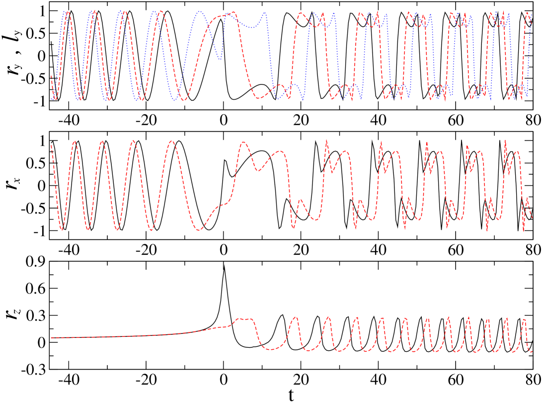
Figure 19: Evolution of right and left movers for a rotor configuration sent in with non-zero transverse velocity. The adiabatic evolution regime where the $\alpha^{\prime}$ expansion holds is clearly visible: the left and right movers evolve periodically in proper time. The solid black and the red dashed lines represents a right mover at $\sigma=\pi/4$ and at one of the end points ($\sigma=0$) respectively. The blue dotted line in the top plot only, describes the left mover at $\sigma=\pi/4$. The third plot shows how the linear momentum on the $z$ direction increases and reaches a value close to the speed of light for points near the string center (solid black line) and remains almost the same for the end point (red dashed line). This is the kink we have discussed previously. The same initial parameters as in Figure 13 were used.

Appendix B Check of numerical evolution

In order to check our numerical algorithm for following the string evolution, we have performed a number of tests. Figure 19 shows the behavior of right and left movers for an incoming rotor. One can readily distinguish the regime of adiabatic oscillations from the super-Hubble evolution around the singularity. In the former region, the right and left movers oscillate as in flat space-time. Different positions $\sigma$ on the string are distinguished only by a phase difference. Moreover, because the rotor is isotropic initially, the incoming $x$ and $y$ components of the right and left movers are equivalent. However, after the singularity these components behave differently, in agreement with the loss of isotropy in the $xy$ plane. Furthermore, the spinning doubled line structure makes the left movers equivalent to the right movers, with only a phase difference. This structure is preserved across the singularity, hence only $\alpha_{n}$, with $n$-odd, are produced during the transition. Contrary, the $z$ direction gets modified during the singularity, from constant right and left movers to a mix of excited states with both, odd and even $n$. In the $1/\alpha^{\prime}$ region, the evolution of right and left movers is completely non-linear and there is not any correlation between right and left movers, between different components and, perhaps more interesting, between different points in the string.

References

- (1) J. Khoury, B. A. Ovrut, P. J. Steinhardt and N. Turok, Phys. Rev. D64 (2001) 123522. [arXiv:hep-th/0103239].
- (2) P. J. Steinhardt and N. Turok, Science 296 (2002) 1436.
- (3) N. Turok, M. Perry and P. J. Steinhardt, Phys. Rev. D70 (2004) 106004.
- (4) J.K. Erickson, D.H. Wesley, P.J. Steinhardt, and N. Turok, Phys. Rev. D69, 063514 (2004); D.H. Wesley, P.J. Steinhardt, and N. Turok, Phys. Rev. D72 063513 (2005).
- (5) A. J. Tolley, [arXiv:hep-th/0505158].
- (6) N. Sanchez (Ed.), String Theory in Curved Spacetimes: A Collaborative Research Report, World Scientific, 1998.
- (7) A similar point is made in H. J. de Vega and N. Sanchez, Phys. Lett. B 197, 320 (1987).
- (8) Even if a cosmological constant is present, solutions of the form (1) still exist in the vicinity of a brane collision turok .
- (9) J. Khoury, B. A. Ovrut, N. Seiberg, P. J. Steinhardt and N. Turok, Phys. Rev. D65 (2002) 086007.
- (10) E. Witten, Nucl. Phys. B471 (1996) 135; Nucl. Phys. B443 (1995) 85.
- (11) A. Lukas, B.A. Ovrut and D. Waldram, Nucl. Phys. B532 (1998) 43; A. Lukas, B.A. Ovrut, K.S. Stelle and D. Waldram, Phys. Rev. D59 (1999) 086001; for a review see B. Ovrut, [arXiv:hep-th/0201032].
- (12) P. McFadden, N. Turok, and P.J. Steinhardt, hep-th/0512123.
- (13) G. Niz and N. Turok, in preparation (2005).
- (14) More precisely, the membrane tension is related to the eleven dimensional gravitational coupling by a quantisation condition relating to the four-form flux mukappa , reading , with an integer.
- (15) M.J. Duff, TASI Lectures, [arXiv:hep-th/9912164].
- (16) N. D. Birrell and P. C. W. Davies, Quantum Fields in Curved Space, CUP, 1982.
- (17) T.W.B. Kibble and N. Turok, Phys. Lett. B116 (1982) 141.
- (18) N. Turok, Nucl. Phys. B242 (1984) 520.
- (19) N. Turok, Phys. Lett. B126 (1983) 437.
- (20) M. Pawlowski, W. Piechocki and M. Spalinski, [arXiv:hep-th/0507142]; P. Malkiewicz and W. Piechocki, [arXiv:gr-qc/0507077].
- (21) D. Kreimer, Nucl. Phys. Proc. Suppl. 89, 289 (2000) [arXiv:hep-th/0005279].
-
(22)
L. Lewin, Polylogarithms and Associated Functions, Elsevier
North Holland, 1981.