Mixing of the RR and NSNS sectors in the BMN limit

Michael B. Green and Aninda Sinha
Department of Applied Mathematics and Theoretical Physics
Wilberforce Road, Cambridge CB3 0WA, UK
E-mail
M.B.Green@damtp.cam.ac.uk, A.Sinha@damtp.cam.ac.uk
   Stefano Kovacs
Max-Planck-Institut für Gravitationsphysik
Albert-Einstein-Institut
Am Mühlenberg 1, D-14476 Potsdam, Germany
E-mail
stefano.kovacs@aei.mpg.de
Abstract:

This paper concerns instanton contributions to two-point correlation functions of BMN operators in ${\mathscr{N}}$=4 supersymmetric Yang–Mills that vanish in planar perturbation theory. Two-point functions of operators with even numbers of fermionic impurities (dual to ${\rm R}\!\otimes\!{\rm R}$ string states) and with purely scalar impurities (dual to ${\rm NS}\!\otimes\!{\rm NS}$ string states) are considered. This includes mixed ${\rm R}\!\otimes\!{\rm R}$ ​​–${\rm NS}\!\otimes\!{\rm NS}$ two-point functions. The gauge theory correlation functions are shown to respect BMN scaling and their behaviour is found to be in good agreement with the corresponding $D$-instanton contributions to two-point amplitudes in the maximally supersymmetric IIB plane-wave string theory. The string theory calculation also shows a simple dependence of the mass matrix elements on the mode numbers of states with an arbitrary number of impurities, which is difficult to extract from the gauge theory. For completeness, a discussion is also given of the perturbative mixing of two-impurity states in the ${\rm R}\!\otimes\!{\rm R}$ and ${\rm NS}\!\otimes\!{\rm NS}$ sectors at the first non-planar level.

preprint: DAMTP-2005-101
AEI-2005-151
hep-th/0512198

1 Introduction and summary

The correspondence between string theory in a maximally supersymmetric IIB plane-wave background [1] and the BMN sector of the ${\mathscr{N}}$=4 supersymmetric Yang–Mills (SYM) theory [2] has been extensively studied at the perturbative level. Non-perturbative aspects of the duality have recently been analysed in [3] and [4], where it was shown that the striking agreement between the effects of $D$-instantons and of Yang–Mills instantons, found in the original formulations of the AdS/CFT correspondence [5, 6, 7], persists in the BMN/plane-wave limit. This paper extends this analysis to include bosonic states with an even number of fermionic impurities in the gauge theory and the corresponding ${\rm R}\!\otimes\!{\rm R}$ states in the dual string theory. The further extension to include fermionic states (which have an odd number of fermionic impurities) involves a straightforward generalisation of these results.

In the BMN limit the gauge theory – string theory correspondence relates the string mass spectrum to the spectrum of scaling dimensions of Yang–Mills gauge invariant operators of large dimension, $\Delta$, and large charge, $J$, with respect to a U(1) subgroup of the SU(4) R-symmetry group. This relation is formally realised via the operator identity

$$\frac{1}{\mu}\,H^{(2)}={\mathcal{D}}-{\mathcal{J}}\,,$$ (1.1)

relating the string theory hamiltonian to the combination ${\mathcal{D}}-{\mathcal{J}}$ of the gauge theory dilation operator and U(1) generator. The duality involves the double limit, $\Delta\to\infty$, $J\to\infty$, with $\Delta-J$ kept finite, on the eigenvalues of the operators ${\mathcal{D}}$ and ${\mathcal{J}}$. The parameter $\mu$ in (1.1) is related to the mass parameter, $m$, entering the light-cone string action by $m=\mu{\alpha^{\prime}}p_{-}$ (where $p_{-}$ is the light-cone momentum) and equals the background value of the ${\rm R}\!\otimes\!{\rm R}$ five-form. The equality (1.1) implies that the eigenvalues of the operators on the two sides should coincide. Numerous tests of this relation have been carried out at the perturbative level [8, 9, 10, 11, 12, 13, 14]. In [3, 4] $D$-instanton contributions to the plane-wave string mass matrix for certain states with up to four bosonic string excitations were shown to be in striking agreement with instanton contributions to the matrix of anomalous dimensions in the corresponding sectors of the dual gauge theory. A brief review of these results is presented in [15].

In the large $N$ limit and in the BMN sector of the gauge theory the rôle of the ordinary ’t Hooft parameters, $\lambda$ and $1/N$, is played by effective rescaled parameters [10, 11],

$$\lambda^{\prime}=\frac{g_{{}_{\rm YM}}^{2}N}{J^{2}}\,,\qquad g_{2}=\frac{J^{2}}{N}\,.$$ (1.2)

In the BMN correspondence these are related to the string parameters via

$$m^{2}=(\mu p_{-}{\alpha^{\prime}})^{2}=\frac{1}{\lambda^{\prime}}\,,\qquad 4\pi g_{\rm s}m^{2}=g_{2}\,,$$ (1.3)

which imply that in the double scaling limit, $N\to\infty$, $J\to\infty$, with $J^{2}/N$ fixed, the weak coupling regime of the gauge theory corresponds to the limit of small $g_{s}$ and large $m$ on the string side.

The string hamiltonian is the sum of two pieces,

$$H^{(2)}=H^{(2)}_{\rm pert}+H^{(2)}_{\rm non-pert}\,.$$ (1.4)

The perturbative part has an expansion in powers of $g_{s}$, which gets reorganised into a series in $g_{2}$. The non-perturbative part contains the $D$-instanton induced corrections. In the BMN limit of the ${\mathscr{N}}$=4 SYM theory, after the operator mixing is resolved [16], quantum corrections to the eigenvalues of ${\mathcal{D}}-{\mathcal{J}}$ are also expected to be organised in a double series in $\lambda^{\prime}$ and $g_{2}$ (a property referred to as BMN scaling), with $g_{2}$ playing the rôle of genus counting parameter. According to [2] the $g_{2}$ expansion in string theory is term by term exact to all orders in $\lambda^{\prime}$. This means that the free string spectrum is identified with the resummed planar expansion of the spectrum of the ${\mathcal{D}}-{\mathcal{J}}$ operator on the gauge side. Loop corrections in string theory correspond to non-planar effects in the Yang–Mills theory. At each order in the loop expansion, the string theory encodes an infinite series of $\lambda^{\prime}$ corrections in the gauge theory at the fixed corresponding order in $g_{2}$.

The large body of work on perturbative and non-perturbative contributions to anomalous dimensions of BMN operators has concentrated almost entirely on states with bosonic impurities. Correspondingly, almost all results on the plane-wave string mass spectrum refer to strings with bosonic excitations. However, fermionic impurities are obviously required in any complete treatment of the mass matrix. States with an even number of fermionic impurities correspond to ${\rm R}\!\otimes\!{\rm R}$ states of the string theory. In general one would expect such states to mix with those containing bosonic impurities, or ${\rm NS}\!\otimes\!{\rm NS}$ states in the string description. Indeed, in [3] it was noted that certain string two-point functions that mix the ${\rm NS}\!\otimes\!{\rm NS}$ and ${\rm R}\!\otimes\!{\rm R}$ sectors receive non-zero $D$-instanton contributions even though these states do not mix at tree level. In this paper we will study these classes of string amplitudes in detail, together with the dual correlation functions in the BMN limit of ${\mathscr{N}}$=4 SYM. The string states and gauge theory operators that we consider contain an arbitrary even number of fermionic and bosonic impurities, but in specific combinations.

On the gauge theory side we find that the two-point functions respect BMN scaling and we determine their dependence on the parameters, $\lambda^{\prime}$ and $g_{2}$, in the semi-classical approximation. Interestingly, we find that, depending on the number and combination of impurities, the result can contain arbitrarily large inverse powers of $\lambda^{\prime}$. The dual string amplitudes, computed using the formalism of [4], are shown to be in very good agreement with the gauge theory results. The string theory calculation also shows a remarkably simple dependence of the mass matrix elements on the mode numbers of states with an arbitrary number of impurities. The dependence on the mode numbers is extremely complicated to determine through a standard instanton calculation in the Yang–Mills theory and thus the string result represents a highly non-trivial prediction for the gauge side.

The mixing of the ${\rm NS}\!\otimes\!{\rm NS}$ and ${\rm R}\!\otimes\!{\rm R}$ sectors can easily be motivated from the presence of background ${\rm R}\!\otimes\!{\rm R}$ flux in the string picture. First note that ${\rm R}\!\otimes\!{\rm R}$ charge conservation is violated in tree-level closed-string scattering from a $D3$-brane, so that ${\rm NS}\!\otimes\!{\rm NS}$ and ${\rm R}\!\otimes\!{\rm R}$ states mix at tree level in AdS${}_{5}\times S^{5}$ (which is the near-horizon geometry of a stack of coincident $D3$-branes). The Penrose boost that takes AdS${}_{5}\times S^{5}$ to the maximally supersymmetric IIB plane-wave background leads to a string theory in which ${\rm R}\!\otimes\!{\rm R}$ charge is conserved on a spherical world-sheet (tree level). However, the non-zero background flux (non-zero $\mu$) leads to the possibility of mixing ${\rm NS}\!\otimes\!{\rm NS}$ and ${\rm R}\!\otimes\!{\rm R}$ states by string loop corrections, as will be indicated later in this paper. This should mean that non-planar perturbative contributions in the gauge theory (i.e. beyond the zeroth order in the $g_{2}$ expansion) mix states that have bosonic impurities with states that have an even number of fermionic impurities. We will later show that this is indeed the case by analysing the leading planar and non-planar contributions to a specific mixed two-point function.

The paper is organised as follows. In section 2 we define the different classes of BMN operators which we focus on and we explain our notation. Section 3 discusses instanton contributions to Yang–Mills two-point functions in the semi-classical approximation. The calculation of the dual $D$-instanton induced amplitudes in string theory is presented in section 4. Section 5 discusses the issue of the perturbative mixing of the ${\rm NS}\!\otimes\!{\rm NS}$ and ${\rm R}\!\otimes\!{\rm R}$ sectors through a qualitative analysis of a specific process.

2 BMN operators

In this section we discuss certain classes of BMN operators whose two-point functions we shall analyse in the following sections. We consider bosonic operators which are SO(4)${}_{C}\times$SO(4)R singlets, corresponding both to ${\rm R}\!\otimes\!{\rm R}$ states, i.e. with an even number of fermionic impurities, and to ${\rm NS}\!\otimes\!{\rm NS}$ states, i.e. containing only bosonic impurities. The operators we consider contain an arbitrary number of impurities, but in certain specific combinations. As will be discussed in the following, in the case of ${\rm R}\!\otimes\!{\rm R}$ states it is convenient to study operators which also contain four bosonic impurities. The inclusion of the bosonic impurities simplifies the analysis in the one-instanton sector because they allow to soak up the fermion superconformal modes without the need to use higher order solutions for any of the fields.

The operators we focus on involve scalar or fermion impurities in singlet combinations. In the BMN limit the four scalars, $\varphi^{i}$, not charged under U(1) transform in the $\left[(0,0);\left(\frac{1}{2},\frac{1}{2}\right)\right]$ of SO(4)${}_{C}\times$SO(4)R. The ${\mathscr{N}}$=4 fermions, $\lambda^{A}_{\alpha}$ and $\bar{\lambda}_{A}^{\dot{\alpha}}$, transforming in the $\mathbf{4}$ and $\mathbf{\bar{4}}$ of SU(4), are decomposed as [4]

$\displaystyle\lambda^{A}_{\alpha}\to\psi^{-\,a}_{\alpha}\oplus\bar{\psi}^{+}_{{\alpha}a}\,,\hskip 28.45274pta=1,4$ (2.1)
$\displaystyle\bar{\lambda}^{\dot{\alpha}}_{A}\to\psi_{\dot{a}}^{+\,{\dot{\alpha}}}\oplus\bar{\psi}^{-\,{\dot{\alpha}}\dot{a}}\,,\hskip 19.91684pt{\dot{a}}=2,3\,,$ (2.2)

where $\psi^{-\,a}_{\alpha}$ and $\psi^{+\,{\dot{\alpha}}}_{\dot{a}}$ have U(1) charge $+\frac{1}{2}$, i.e. $\Delta-J=1$, whereas $\bar{\psi}^{+}_{{\alpha}a}$ and $\bar{\psi}^{-\,{\dot{\alpha}}\dot{a}}$ have charge $-\frac{1}{2}$, i.e. $\Delta-J=2$. Under the SO(4)${}_{C}\times$SO(4)R symmetry the fermions $\psi^{-\,a}_{\alpha}$ and $\bar{\psi}^{+}_{{\alpha}a}$ transform in the $\left[\left(\frac{1}{2},0\right);\left(\frac{1}{2},0\right)\right]$, while $\psi_{\dot{a}}^{+\,{\dot{\alpha}}}$ and $\bar{\psi}^{-\,{\dot{\alpha}}\dot{a}}$ transform in the $\left[\left(0,\frac{1}{2}\right);\left(0,\frac{1}{2}\right)\right]$. The definition of the fermions $\bar{\psi}^{+}_{{\alpha}a}$ and $\bar{\psi}^{-\,{\dot{\alpha}}\dot{a}}$ involves the multiplication by a matrix which flips the SO(4)R chirality and respectively lowers or raises the corresponding index. The decomposition in (2.1)-(2.2) corresponds to the decomposition of the left- and right-moving type IIB fermions into chiral SO(4)${}_{C}\times$SO(4)R fermions [17, 18], $(S^{-},S^{+})$ and $(\tilde{S}^{-},\tilde{S}^{+}$).

Fermion impurities in BMN operators are associated with the insertion of the $\Delta-J=1$ fields, $\psi^{-\,a}_{\alpha}$ and $\psi^{+\,{\dot{\alpha}}}_{\dot{a}}$. In the dual string theory this corresponds to the insertion of $S^{-}_{-n}$ and $S^{+}_{-n}$ (or $\tilde{S}^{-}_{-n}$ and $\tilde{S}^{+}_{-n}$) creation operators. The conjugate fermions, $\bar{\psi}^{+}_{{\alpha}a}$ and $\bar{\psi}^{-\,{\dot{\alpha}}\dot{a}}$, which have $\Delta-J=2$, enter into the conjugate operators. In perturbation theory the only non-zero contractions are between a fermion and its conjugate, i.e. $\langle\psi^{-\,a}_{\alpha}\bar{\psi}^{-\,{\dot{\beta}}\dot{b}}\rangle$ and $\langle\psi^{+\,{\dot{\alpha}}}_{\dot{a}}\bar{\psi}^{+}_{\beta b}\rangle$. This will be important in the analysis of correlation functions in the next sections.

The most general BMN operator with fermionic impurities that we shall consider is of the form

$\displaystyle{\mathscr{O}}^{k,h}_{\bm{\ell},\bm{n},\bm{m}}$ $\displaystyle=$ $\displaystyle t_{\bm{i},\bm{a},\bm{{\dot{\beta}}}}^{{\scriptscriptstyle({\rm R}\otimes{\rm R})}\,\bm{{\dot{b}}},\bm{\alpha}}\>c_{k,h}(g_{{}_{\rm YM}},N,J)$ (2.6)
$\displaystyle\!\times\!$ $\displaystyle\begin{array}[t]{c}{\displaystyle\sum_{p_{2},p_{3},p_{4},u_{1},\dots,v_{2h}=0}^{J}}\\ {\scriptstyle p_{2}+p_{3}+p_{4}+u_{1}+\cdots+v_{2h}\leq J}\\ {\scriptstyle p_{1}=J-(p_{2}+p_{3}+p_{4}+u_{1}+\cdots+v_{2h})}\end{array}e(\bm{p},\bm{u},\bm{v};\bm{\ell},\bm{n},\bm{m};J)\>{\rm Tr}\left[{\mathcal{Z}}^{(\bm{p},\bm{i})}_{\varphi}{\mathcal{Z}}^{(\bm{u},\bm{\alpha},\bm{a})}_{\psi^{-}}{\mathcal{Z}}^{(\bm{v},\bm{{\dot{\beta}}},\bm{{\dot{b}}})}_{\psi^{+}}\right],\rule{0.0pt}{16.0pt}$

where various sets of indices have been grouped into ‘vectors’,

$\displaystyle\bm{p}=(p_{1},p_{2},p_{3},p_{4})\,,\hskip 40.68723pt\bm{u}=(u_{1},u_{2},\ldots,u_{2k})\,,\hskip 38.41139pt\bm{v}=(v_{1},v_{2},\ldots,v_{2h})\,,$
$\displaystyle\bm{\ell}=(\ell_{1},\ell_{2},\ell_{3})\,,\hskip 60.03532pt\bm{n}=(n_{1},n_{2},\ldots,n_{2k})\,,\hskip 36.98866pt\bm{m}=(m_{1},m_{2},\ldots,m_{2h})\,,$
$\displaystyle\bm{i}=(i_{1},i_{2},i_{3},i_{4})\,,\hskip 50.07669pt\bm{a}=(a_{1},a_{2},\ldots,a_{2k})\,,\hskip 41.25641pt\bm{{\dot{b}}}=(\dot{b}_{1},\dot{b}_{2},\ldots,\dot{b}_{2h})$
$\displaystyle\bm{{\alpha}}=({\alpha}_{1},{\alpha}_{2},\ldots,{\alpha}_{2k})\,,\hskip 26.17648pt\bm{{\dot{\beta}}}=({\dot{\beta}}_{1},{\dot{\beta}}_{2},\ldots,{\dot{\beta}}_{2h})\,,$ (2.7)

and we have introduced the notation

$${\mathcal{Z}}_{\varphi}^{(\bm{p},\bm{i})}=\prod_{r=1}^{4}Z^{p_{r}}\varphi^{i_{r}}\,,\qquad{\mathcal{Z}}_{\psi^{-}}^{(\bm{u},\bm{\alpha},\bm{a})}=\prod_{r=1}^{2k}Z^{u_{r}}\psi^{-\,a_{r}}_{{\alpha}_{r}}\,,\qquad{\mathcal{Z}}_{\psi^{+}}^{(\bm{v},\bm{{\dot{\beta}}},\bm{{\dot{b}}})}=\prod_{r=1}^{2h}Z^{v_{r}}\psi^{+\,{\dot{\beta}}_{r}}_{\dot{b}_{r}}\,.$$ (2.8)

The coefficient $e(\bm{p},\bm{u},\bm{v};\bm{\ell},\bm{n},\bm{m};J)$ in (2.6) is given by

$\displaystyle e(\bm{p},\bm{u},\bm{v};\bm{\ell},\bm{n},\bm{m};J)=\exp\left\{2\pi i[p_{2}(\ell_{1}+\cdots+m_{2h})+p_{3}(\ell_{2}+\cdots+m_{2h})\right.$
$\displaystyle\hskip 28.45274pt+p_{4}(\ell_{3}+\cdots+m_{2h})+u_{1}(n_{1}+\cdots+m_{2h})+\cdots+u_{2k}(n_{2k}+\cdots+m_{2h})$
$\displaystyle\hskip 27.03003pt\left.+v_{1}(m_{1}+\cdots+m_{2h})+\cdots+v_{2h}m_{2h}]/J\right\}\,.$

The tensor $t_{\bm{i},\bm{a},\bm{{\dot{\beta}}}}^{{\scriptscriptstyle({\rm R}\otimes{\rm R})}\,\bm{{\dot{b}}},\bm{\alpha}}$ projects onto the SO(4)R singlet,

$$t_{\bm{i},\bm{a},\bm{{\dot{\beta}}}}^{{\scriptscriptstyle({\rm R}\otimes{\rm R})}\,\bm{{\dot{b}}},\bm{\alpha}}=\varepsilon_{i_{1}i_{2}i_{3}i_{4}}\,\prod_{r=1}^{k}\varepsilon_{a_{2r-1}a_{2r}}\varepsilon^{{\alpha}_{2r-1}{\alpha}_{2r}}\,\prod_{s=1}^{h}\varepsilon^{\dot{b}_{2s-1}\dot{b}_{2s}}\varepsilon_{{\dot{\beta}}_{2s-1}{\dot{\beta}}_{2s}}$$ (2.9)

and the normalisation coefficient, $c_{k,h}(g_{{}_{\rm YM}},N,J)$, is

$$c_{k,h}(g_{{}_{\rm YM}},N,J)=\frac{1}{\sqrt{J^{3+2k+2h}\left(\frac{g_{{}_{\rm YM}}^{2}N}{8\pi^{2}}\right)^{J+4+2k+2h}}}\,.$$ (2.10)

The form of the conjugate operator is similar to (2.6) with the $Z$’s replaced by ${\bar{Z}}$’s and the $\psi^{-}$’s and $\psi^{+}$’s replaced respectively by $\bar{\psi}^{-}$’s and $\bar{\psi}^{+}$s’. In the following we shall consider two-point functions of the form $\langle{\mathscr{O}}^{k,h}_{\bm{\ell},\bm{n},\bm{m}}(x_{1})\,\bar{\mathscr{O}}^{k^{\prime},h^{\prime}}_{\bm{\ell}^{\prime},\bm{n}^{\prime},\bm{m}^{\prime}}(x_{2})\rangle$, where the operator ${\mathscr{O}}^{k,h}_{\bm{\ell},\bm{n},\bm{m}}$ contains $k$ $\psi^{-}$ and $h$ $\psi^{+}$ pairs and the operator $\bar{\mathscr{O}}^{k^{\prime},h^{\prime}}_{\bm{\ell}^{\prime},\bm{n}^{\prime},\bm{m}^{\prime}}$ contains $k^{\prime}$ $\bar{\psi}^{-}$ and $h^{\prime}$ $\bar{\psi}^{+}$ pairs. The normalisation of the operators is such that two-point functions of this type (if non-zero) are of order 1 at tree level.

The string states which we are interested in, dual to operators of the form (2.6), are schematically, up to an overall normalisation, of the form (see [3] for notation)

$$\varepsilon_{i_{1}i_{2}i_{3}i_{4}}\,{\alpha}^{i_{1}}_{-\ell_{1}}{\alpha}^{i_{2}}_{-\ell_{2}}\tilde{\alpha}^{i_{3}}_{-\ell_{1}}\tilde{\alpha}^{i_{4}}_{-\ell_{2}}\left[S^{-}_{-n_{1}}\tilde{S}^{-}_{-n_{1}}\right]\ldots\left[S^{-}_{-n_{k}}\tilde{S}^{-}_{-n_{k}}\right]\!\left[S^{+}_{-m_{1}}\tilde{S}^{+}_{-m_{1}}\right]\ldots\left[S^{+}_{-m_{h}}\tilde{S}^{+}_{-m_{h}}\right]|0\rangle_{h}\,,$$ (2.11)

where $|0\rangle_{h}$ denotes the BMN ground state and the square brackets indicate contraction of the SO(4)${}_{C}\times$SO(4)R indices. Notice that in (2.11) we have inserted the same number of left- and right-moving oscillators and we have chosen the mode numbers carried by the creation operators to be equal in pairs. More general states satisfying the physical level-matching condition can be constructed, but we restrict our attention to those of the form (2.11) because these form a class of states that couple to a $D$-instanton in the plane-wave background.

In the operator (2.6) $k$ pairs of $\psi^{-}$ fermions and $h$ pairs of $\psi^{+}$ fermions are contracted into SO(4)${}_{C}\times$SO(4)R singlets. In the operator $\bar{\mathscr{O}}^{k^{\prime},h^{\prime}}_{\bm{\ell}^{\prime},\bm{n}^{\prime},\bm{m}^{\prime}}$ the $2k^{\prime}$ $\bar{\psi}^{-}$’s and the $2h^{\prime}$ $\bar{\psi}^{+}$’s are similarly paired in singlets. The unique singlet that can be constructed in this way involves contractions of both types of SO(4) indices via $\varepsilon$ tensors, see (2.9). This implies that the fermions are automatically pairwise antisymmetrised in the colour indices. In the string state (2.11) there is no analogue of the colour antisymmetrisation, but the contraction is allowed because the two fermions in each pair are different, being a left- and a right-mover.

The other class of operators we consider are dual to string states in the ${\rm NS}\!\otimes\!{\rm NS}$ sector. These involve an arbitrary number of scalar impurities contracted into a SO(4)${}_{C}\times$SO(4)R singlet. Using the same notation introduced in (2.6) the operators are

$${\mathscr{O}}^{l}_{\bm{\ell},\bm{n}}=t_{\bm{i},\bm{j}}^{\scriptscriptstyle({\rm NS}\otimes{\rm NS})}\>c_{l}(g_{{}_{\rm YM}},N,J+l)\begin{array}[t]{c}{\displaystyle\sum_{p_{2},p_{3},p_{4},q_{1},\dots,q_{2l}=0}^{J+l}}\\ {\scriptstyle p_{2}+p_{3}+p_{4}+q_{1}+\cdots+q_{2l}\leq J+l}\\ {\scriptstyle p_{1}=J+l-(p_{2}+p_{3}+p_{4}+q_{1}+\cdots+q_{2l})}\end{array}e(\bm{p},\bm{q};\bm{\ell},\bm{n};J+l)\;{\rm Tr}\left[{\mathcal{Z}}^{(\bm{p},\bm{i})}_{\varphi}{\mathcal{Z}}^{(\bm{q},\bm{j})}_{\varphi}\right],\rule{0.0pt}{16.0pt}$$ (2.12)

where a vector notation for the indices has been used,

$\displaystyle\bm{p}=(p_{1},p_{2},p_{3},p_{4})\,,\hskip 40.68723pt\bm{q}=(q_{1},q_{2},\ldots,q_{2l})\,,$
$\displaystyle\bm{\ell}=(\ell_{1},\ell_{2},\ell_{3})\,,\hskip 60.03532pt\bm{n}=(n_{1},n_{2},\ldots,n_{2l})\,,$
$\displaystyle\bm{i}=(i_{1},i_{2},i_{3},i_{4})\,,\hskip 50.07669pt\bm{j}=(j_{1},j_{2},\ldots,j_{2l})\,.$ (2.13)

The tensor $t_{\bm{i},\bm{j}}^{\scriptscriptstyle({\rm NS}\otimes{\rm NS})}$, which projects onto the SO(4)R singlet, is

$$t_{\bm{i},\bm{j}}^{\scriptscriptstyle({\rm NS}\otimes{\rm NS})}=\varepsilon_{i_{1}i_{2}i_{3}i_{4}}\,\delta_{j_{1}j_{2}}\delta_{j_{3}j_{4}}\cdots\delta_{j_{2l-1}j_{2l}}\,,$$ (2.14)

i.e. we choose singlet operators in which four scalars are contracted via an $\varepsilon$-tensor and the remaining $2l$ scalars are contracted pairwise via Kronecker $\delta$’s. The normalisation factor in (2.12) is

$$c_{l}(g_{{}_{\rm YM}},N,J+l)=\frac{1}{\sqrt{J^{3+2l}\left(\frac{g_{{}_{\rm YM}}^{2}N}{8\pi^{2}}\right)^{J+4+3l}}}\,$$ (2.15)

and the phase factor in the sum, $e(\bm{p},\bm{q};\bm{\ell},\bm{n};J+l)$, is

$\displaystyle e(\bm{p},\bm{q};\bm{\ell},\bm{n};J+l)$ $\displaystyle=$ $\displaystyle\exp\left\{2\pi i[p_{2}(\ell_{1}+\cdots+n_{2l})+p_{3}(\ell_{2}+\cdots+n_{2l})+p_{4}(\ell_{3}+\cdots+n_{2l})\right.$ (2.16)
$\displaystyle+$ $\displaystyle\left.q_{1}(n_{1}+\cdots+n_{2l})+\cdots+q_{2l}n_{2l}]/J\right\}\,.$

Notice that the operator (2.12) contains a total of $J+l$ $Z$ fields. This is necessary in order to give it the same dimension and U(1) charge as operators with a total of $2l$ fermionic impurities ($\psi^{-}$ and/or $\psi^{+}$) of the type defined in (2.6). The number of $Z$’s in the operator is reflected in the power of $g_{{}_{\rm YM}}^{2}N/8\pi^{2}$ in the normalisation (2.15).

The string states dual to operators of the form (2.12) are (up to a normalisation factor)

$$\varepsilon_{i_{1}i_{2}i_{3}i_{4}}\,{\alpha}^{i_{1}}_{-\ell_{1}}{\alpha}^{i_{2}}_{-\ell_{2}}\tilde{\alpha}^{i_{3}}_{-\ell_{1}}\tilde{\alpha}^{i_{4}}_{\ell_{2}}{\alpha}^{j_{1}}_{-n_{1}}\tilde{\alpha}^{j_{1}}_{-n_{1}}{\alpha}^{j_{2}}_{-n_{2}}\tilde{\alpha}^{j_{2}}_{-n_{2}}\cdots{\alpha}^{j_{l}}_{-n_{l}}\tilde{\alpha}^{j_{l}}_{-n_{l}}|0\rangle_{h}\,,$$ (2.17)

where, as in the case of the ${\rm R}\!\otimes\!{\rm R}$ state (2.11), we have restricted the attention to a class of states that couple to a $D$-instanton in the plane-wave background: the number of left- and right-movers in (2.17) is the same and the corresponding mode numbers are equal in pairs.

In order to construct gauge theory operators that can be identified with the string states (2.11) and (2.17) one needs to consider linear combinations of operators such as those defined in (2.6) in (2.12). Since the creation operators in the string states commute, it is necessary to sum, in the corresponding operators, over all the possible permutations of the $\varphi$ and $\psi^{\pm}$ impurities. As in the four impurity case studied in [4] it is also necessary to (anti-)symmetrise the operators under permutations of the mode numbers so that they possess the same symmetry properties as the dual string states. This should automatically impose the constraint that the instanton contribution vanishes unless the mode numbers in the operator are equal in pairs as in (2.11) and (2.17). We shall not discuss these aspects here since we shall not analyse the mode number dependence in the gauge theory two-point functions.

The insertion of $\Delta-J=2$ impurities is, in general, necessary to define well-behaved BMN operators, as observed already in the case of two impurity operators in [12, 19]. This is also the case for operators in the class we are considering. Specifically, the complete definition of the operators should also involve terms with $\bar{\psi}^{+}_{{\alpha}a}$ and $\bar{\psi}^{-\,{\dot{\alpha}}a}$ insertions as well as terms in which pairs of $\varphi$’s in a singlet are replaced by a $Z{\bar{Z}}$ insertion. However, these terms are not relevant at leading order in the large $J$ and large $N$ limit and only need to be taken into account when $g_{2}$ corrections are computed, i.e. beyond the semi-classical approximation.

3 Gauge theory two-point functions in the one-instanton sector

In this section we briefly review the calculation of one-instanton contributions to two-point correlation functions in semi-classical approximation and then discuss examples involving the operators defined in the previous section.

3.1 Semi-classical approximation

The one-instanton contribution to the two-point correlation function of composite operators ${\mathscr{O}}_{1}$ and ${\mathscr{O}}_{2}$ in the semi-classical approximation takes the form

$$G^{\rm 1-inst}(x_{1},x_{2})=\int{\rm d}\mu_{\rm inst}({\mathpzc m}_{\rm\,b},{\mathpzc m}_{\rm\,f})\,{\rm e}^{-S_{\rm inst}}\;\,\widehat{\mathscr{O}}_{1}(x_{1};{\mathpzc m}_{\rm\,b},{\mathpzc m}_{\rm\,f})\;\widehat{\mathscr{O}}_{2}(x_{2};{\mathpzc m}_{\rm\,b},{\mathpzc m}_{\rm\,f})\,,$$ (3.1)

where we have denoted the bosonic and fermionic collective coordinates by ${\mathpzc m}_{\rm\,b}$ and ${\mathpzc m}_{\rm\,f}$ respectively. In (3.1) ${\rm d}\mu_{\rm inst}({\mathpzc m}_{\rm\,b},{\mathpzc m}_{\rm\,f})$ is the integration measure on the instanton moduli space, $S_{\rm inst}$ is the classical action evaluated on the instanton solution and $\widehat{\mathscr{O}}_{1}$ and $\widehat{\mathscr{O}}_{2}$ denote the classical expressions for the operators computed in the instanton background. In the case of gauge-invariant operators the semi-classical expression (3.1) involves the integration over the position and size of the instanton, $x_{0}$ and $\rho$, and over the sixteen fermion moduli associated with the broken supersymmetries, $\eta^{A}$ and $\bar{\xi}^{A}$. The bosonic moduli associated with global gauge orientations are integrated out. The corresponding fermion moduli, $\nu^{A}$ and $\bar{\nu}^{A}$, appear in gauge-invariant operators in colour-singlet bilinears and the integration over these moduli is re-expressed in terms of an integration over bosonic auxiliary variables, $\Omega^{AB}$, parametrising a five-sphere. Instanton contributions to two-point functions of scalar operators in ${\mathscr{N}}$=4 SYM have been analysed in [20]. Details of the calculation of two-point functions of BMN operators were discussed in [4] following the general analysis of [6]. Comprehensive reviews of instanton calculus in supersymmetric gauge theories can be found in [21, 22, 23]. For a generic two-point function one finds

$\displaystyle\langle{\mathscr{O}}_{1}(x_{1})\,{\mathscr{O}}_{2}(x_{2})\rangle={\alpha}(p,q,N)\,g_{{}_{\rm YM}}^{8+p+q}\,{\rm e}^{2\pi i\tau}\int{\rm d}\rho\,{\rm d}^{4}x_{0}\,{\rm d}^{5}\Omega\prod_{A=1}^{4}{\rm d}^{2}\eta^{A}{\rm d}^{2}\bar{\xi}^{A}\,\rho^{p+q-5}$
$\displaystyle\times\widehat{\mathscr{O}}_{1}(x_{1};\rho,x_{0},\Omega,\eta,\bar{\xi})\;\widehat{\mathscr{O}}_{2}(x_{2};\rho,x_{0},\Omega,\eta,\bar{\xi})$ $\displaystyle\!\!,$ (3.2)

where the $\bar{\nu}^{A}\nu^{B}$ bilinears in the operator profiles have been re-written in terms of the auxiliary variables $\Omega^{AB}$. In the large-$N$ limit

$${\alpha}(p,q,N)\sim\frac{N^{\frac{1}{2}(p+1)}}{\pi^{p+q+\frac{1}{2}}}\left[1+O(1/N)\right]\,,$$ (3.3)

where $p$ and $q$ are the numbers of antisymmetric and symmetric $\bar{\nu}^{A}\nu^{B}$ bilinears respectively.

In all the examples that we shall consider the classical profiles of the operators take a factorised form. In such expressions the terms which contribute to two-point functions can be written schematically as

$$\widehat{\mathscr{O}}(x;x_{0},\rho,\eta,\bar{\xi},\Omega)\sim f(x;x_{0},\rho)\,g(\Omega)\prod_{A=1}^{4}\left[\zeta^{A}(x)\right]^{2}\,,$$ (3.4)

where $\zeta^{A}$ is a combination of the fermion modes, $\eta^{A}$ and $\bar{\xi}^{A}$, associated with the broken superconformal symmetries,

$$\zeta^{A}_{\alpha}(x)=\frac{1}{\sqrt{\rho}}\left[\rho\,\eta^{A}_{\alpha}-(x-x_{0})_{\mu}\sigma^{\mu}_{{\alpha}{\dot{\alpha}}}\bar{\xi}^{{\dot{\alpha}}A}\right]\,.$$ (3.5)

The generic two-point function thus becomes

$\displaystyle\langle{\mathscr{O}}_{1}(x_{1})\,{\mathscr{O}}_{2}(x_{2})\rangle_{\rm inst}$ $\displaystyle\sim$ $\displaystyle{\alpha}(p,q,N)\,g_{{}_{\rm YM}}^{8+p+q}\,{\rm e}^{2\pi i\tau}\int{\rm d}\rho\,{\rm d}^{4}x_{0}\,\rho^{p+q-5}\,f_{1}(x_{1};x_{0},\rho)\,f_{2}(x_{2};x_{0},\rho)$ (3.6)
$\displaystyle\times$ $\displaystyle\int{\rm d}^{8}\eta\,{\rm d}^{8}\bar{\xi}\,\prod_{A=1}^{4}\left[\zeta^{A}(x_{1})\right]^{2}\left[\zeta^{A}(x_{2})\right]^{2}\int{\rm d}^{5}\Omega\,g_{1}(\Omega)\,g_{2}(\Omega)\,.$

After this factorisation the bosonic integration over $x_{0}$ and $\rho$ is logarithmically divergent and needs to be regularised. This signals a contribution to the matrix of anomalous dimensions which is extracted from the coefficient of the logarithmically divergent term.

The integration over the superconformal modes in the second line of (3.6) is straightforward,

$$\int{\rm d}^{8}\eta\,{\rm d}^{8}\bar{\xi}\,\prod_{A=1}^{4}\left[\zeta^{A}(x_{1})\right]^{2}\left[\zeta^{A}(x_{2})\right]^{2}=(x_{1}-x_{2})^{8}\,.$$ (3.7)

Finally, as will be shown in the next section, the five-sphere integrals in all the cases we are interested in can be reduced to the form

$$I_{S^{5}}(a,b,c)=\int{\rm d}^{5}\Omega\,\left(\Omega^{14}\Omega^{23}\right)^{a}\left(\Omega^{12}\Omega^{34}\right)^{b}\left(\Omega^{13}\Omega^{24}\right)^{c}\,,$$ (3.8)

where $a$, $b$ and $c$ are integers. This integral is a generalisation of those encountered in the case of two and four impurity operators and can be evaluated using the same method described in [4]. Defining

$\displaystyle\Omega=\Sigma^{14}_{i}\Omega^{i}=\Omega^{1}+i\Omega^{4}\,,\qquad\bar{\Omega}=\Sigma^{23}_{i}\Omega^{i}=\Omega^{1}-i\Omega^{4}\,,$
$\displaystyle\widetilde{\Omega}=\Sigma^{12}_{i}\Omega^{i}=\Omega^{3}+i\Omega^{6}\,,\qquad\bar{\widetilde{\Omega}}=\Sigma^{34}_{i}\Omega^{i}=\Omega^{3}-i\Omega^{6}\,,$
$\displaystyle\widehat{\Omega}=\Sigma^{13}_{i}\Omega^{i}=\Omega^{2}+i\Omega^{5}\,,\qquad\bar{\widehat{\Omega}}=\Sigma^{24}_{i}\Omega^{i}=\Omega^{2}-i\Omega^{5}\,,$ (3.9)

the integral (3.8) can be rewritten as

$$I_{S^{5}}(a,b,c)=\int{\rm d}\Omega{\rm d}\bar{\Omega}{\rm d}\widetilde{\Omega}{\rm d}\bar{\widetilde{\Omega}}{\rm d}\widehat{\Omega}{\rm d}\bar{\widehat{\Omega}}\,\delta(\Omega\bar{\Omega}+\widetilde{\Omega}\bar{\widetilde{\Omega}}+\widehat{\Omega}\bar{\widehat{\Omega}}-1)\,\left(\Omega\bar{\Omega}\right)^{a}\left(\widetilde{\Omega}\bar{\widetilde{\Omega}}\right)^{b}\left(\widehat{\Omega}\bar{\widehat{\Omega}}\right)^{c}\,.$$ (3.10)

This can be easily computed generalising the calculations of [4]. The result is

$$I_{S^{5}}(a,b,c)=\pi^{3}\,\frac{\Gamma(a+1)\,\Gamma(b+1)\,\Gamma(c+1)}{\Gamma(a+b+c+3)}\,.$$ (3.11)

In the next subsections we shall apply this general analysis to certain classes of two-point functions of the operators introduced in section 2.

3.2 A class of two-point functions in the ${\rm R}\!\otimes\!{\rm R}$ sector

In this section we analyse the one-instanton contribution to two-point functions of the operators ${\mathscr{O}}^{k,h}_{\bm{\ell},\bm{n},\bm{m}}$ and $\bar{\mathscr{O}}^{k^{\prime},h^{\prime}}_{\bm{\ell}^{\prime},\bm{n}^{\prime},\bm{m}^{\prime}}$ defined in section 2. The generic two-point function in this class is

$$G^{k,h;k^{\prime},h^{\prime}}_{\bm{\ell},\bm{n},\bm{m};\bm{\ell}^{\prime},\bm{n}^{\prime},\bm{m}^{\prime}}(x_{1},x_{2})=\langle{\mathscr{O}}^{k,h}_{\bm{\ell},\bm{n},\bm{m}}(x_{1})\bar{\mathscr{O}}^{k^{\prime},h^{\prime}}_{\bm{\ell}^{\prime},\bm{n}^{\prime},\bm{m}^{\prime}}(x_{2})\rangle\,,$$ (3.12)

where conformal invariance and conservation of $J$ require $k+h=k^{\prime}+h^{\prime}$.

The combinatorics involved in the calculation of (3.12) is rather formidable and we shall not present a detailed computation of the complete two-point functions. However, our analysis will be sufficient to determine the dependence of the two-point functions in this class on the parameters $g_{{}_{\rm YM}}$, $N$ and $J$, which will be compared with the result of the dual string amplitude in section 4.

As previously observed, the only non-zero free fermion propagators are $\langle\psi^{-\,a}_{\alpha}\bar{\psi}^{-\,{\dot{\beta}}\dot{b}}\rangle$ and $\langle\psi^{+\,{\dot{\alpha}}}_{\dot{a}}\bar{\psi}^{+}_{\beta b}\rangle$. This implies that the two-point functions in the class (3.12) are only non-zero at tree level if $k=k^{\prime}$ and $h=h^{\prime}$. We will now show that instanton contributions to these correlation functions are non-zero, in the leading semi-classical approximation, if the weaker condition $k+h=k^{\prime}+h^{\prime}$ imposed by the symmetries is satisfied.

The dependence on the parameters, $g_{{}_{\rm YM}}$, $N$ and $J$, in the two-point function (3.12) can be determined analysing the structure of the fermion zero modes in the classical profiles of the operators in the instanton background. The combinations of scalar impurities entering into ${\mathscr{O}}^{k,h}_{\bm{\ell},\bm{n},\bm{m}}$ and $\bar{\mathscr{O}}^{k^{\prime},h^{\prime}}_{\bm{\ell}^{\prime},\bm{n}^{\prime},\bm{m}^{\prime}}$ are

$\displaystyle+\varphi^{12}\varphi^{13}\varphi^{24}\varphi^{34}\,,\quad-\varphi^{12}\varphi^{34}\varphi^{24}\varphi^{13}\,,\quad+\varphi^{12}\varphi^{24}\varphi^{34}\varphi^{13}\,,$
$\displaystyle+\varphi^{12}\varphi^{34}\varphi^{13}\varphi^{24}\,,\quad-\varphi^{12}\varphi^{13}\varphi^{34}\varphi^{24}\,,\quad-\varphi^{12}\varphi^{24}\varphi^{13}\varphi^{34}\,,$ (3.13)

and cyclic permutations of these. All the terms in (3.13) contain the same combination of fermion zero modes,

$$\left({\mathpzc m}_{\rm\,f}^{1}\right)^{2}\left({\mathpzc m}_{\rm\,f}^{2}\right)^{2}\left({\mathpzc m}_{\rm\,f}^{3}\right)^{2}\left({\mathpzc m}_{\rm\,f}^{4}\right)^{2}\,,$$ (3.14)

where ${\mathpzc m}_{\rm\,f}^{A}$ indicates a generic fermion zero mode in the one-instanton sector, i.e. either a superconformal mode, $\eta^{A}$ or $\bar{\xi}^{A}$, or a mode of type $\nu^{A}$ or $\bar{\nu}^{A}$.

The zero modes contained in the pairs of fermionic impurities in ${\mathscr{O}}^{k,h}_{\bm{\ell},\bm{n},\bm{m}}$ are

$\displaystyle\varepsilon_{ab}\,\psi^{-\,{\alpha}a}\psi_{a}^{-\,b}\sim{\mathpzc m}_{\rm\,f}^{1}{\mathpzc m}_{\rm\,f}^{4}$
$\displaystyle\varepsilon^{\dot{a}\dot{b}}\,\psi^{+}_{{\dot{\alpha}}\dot{a}}\psi^{+\,{\dot{\alpha}}}_{\dot{b}}\sim\left({\mathpzc m}_{\rm\,f}^{1}\right)^{2}{\mathpzc m}_{\rm\,f}^{2}{\mathpzc m}_{\rm\,f}^{3}\left({\mathpzc m}_{\rm\,f}^{4}\right)^{2}\,.$ (3.15)

Similarly the fermionic impurities in $\bar{\mathscr{O}}^{k^{\prime},h^{\prime}}_{\bm{\ell}^{\prime},\bm{n}^{\prime},\bm{m}^{\prime}}$ contain

$\displaystyle\varepsilon_{\dot{a}\dot{b}}\,\bar{\psi}^{-\,\dot{a}}_{\dot{\alpha}}\bar{\psi}^{-\,{\dot{\alpha}}\dot{b}}\sim{\mathpzc m}_{\rm\,f}^{1}\left({\mathpzc m}_{\rm\,f}^{2}\right)^{2}\left({\mathpzc m}_{\rm\,f}^{3}\right)^{2}{\mathpzc m}_{\rm\,f}^{4}$
$\displaystyle\varepsilon^{ab}\,\bar{\psi}^{+\,{\alpha}}_{a}\bar{\psi}^{+}_{{\alpha}b}\sim{\mathpzc m}_{\rm\,f}^{2}{\mathpzc m}_{\rm\,f}^{3}\,.$ (3.16)

Taking into account the $J$ $Z$ fields in ${\mathscr{O}}$ and the $J$ ${\bar{Z}}$ fields in $\bar{\mathscr{O}}$ the two operators contain the following combinations of fermion modes

$\displaystyle\widehat{\mathscr{O}}^{k,h}_{\bm{\ell},\bm{n},\bm{m}}$ $\displaystyle\to$ $\displaystyle\left({\mathpzc m}_{\rm\,f}^{1}\right)^{J+2+k+2h}\left({\mathpzc m}_{\rm\,f}^{2}\right)^{2+h}\left({\mathpzc m}_{\rm\,f}^{3}\right)^{2+h}\left({\mathpzc m}_{\rm\,f}^{4}\right)^{J+2+k+2h}$
$\displaystyle\widehat{\!\!\bar{\mathscr{O}}}^{k^{\prime},h^{\prime}}_{\bm{\ell}^{\prime},\bm{n}^{\prime},\bm{m}^{\prime}}$ $\displaystyle\to$ $\displaystyle\left({\mathpzc m}_{\rm\,f}^{1}\right)^{2+k^{\prime}}\left({\mathpzc m}_{\rm\,f}^{2}\right)^{J+2+2k^{\prime}+h^{\prime}}\left({\mathpzc m}_{\rm\,f}^{3}\right)^{J+2+2k^{\prime}+h^{\prime}}\left({\mathpzc m}_{\rm\,f}^{4}\right)^{2+k^{\prime}}\,.$ (3.17)

The computation of the two-point function $G^{k,h;k^{\prime},h^{\prime}}_{\bm{\ell},\bm{n},\bm{m};\bm{\ell}^{\prime},\bm{n}^{\prime},\bm{m}^{\prime}}(x_{1},x_{2})$ in the semi-classical approximation involves the integration over the sixteen fermion superconformal modes associated with the broken Poincaré and special supersymmetries. To saturate these integrations the two operators must both contain $\prod_{A=1}^{4}\left(\zeta^{A}\right)^{2}$, where $\zeta^{A}_{\alpha}=\frac{1}{\sqrt{\rho}}[\rho\eta^{A}_{\alpha}-(x-x_{0})_{\mu}\sigma^{\mu}_{{\alpha}{\dot{\alpha}}}\bar{\xi}^{{\dot{\alpha}}A}]$. This requirement combined with (3.17) implies that in the product of the profiles of the two operators one must select terms containing

$\displaystyle\widehat{\mathscr{O}}^{k,h}_{\bm{\ell},\bm{n},\bm{m}}(x_{1})\;\;\widehat{\!\!\bar{\mathscr{O}}}^{k^{\prime},h^{\prime}}_{\bm{\ell}^{\prime},\bm{n}^{\prime},\bm{m}^{\prime}}(x_{2})\to\left[\left(\zeta^{1}\right)^{2}\left(\zeta^{2}\right)^{2}\left(\zeta^{3}\right)^{2}\left(\zeta^{4}\right)^{2}\right]\!(x_{1})\left[\left(\zeta^{1}\right)^{2}\left(\zeta^{2}\right)^{2}\left(\zeta^{3}\right)^{2}\left(\zeta^{4}\right)^{2}\right]\!(x_{2})$
$\displaystyle\times\left(\nu^{1}+\bar{\nu}^{1}\right)^{J+k+2h+k^{\prime}}\left(\nu^{2}+\bar{\nu}^{2}\right)^{J+h+2k^{\prime}+h^{\prime}}\left(\nu^{3}+\bar{\nu}^{3}\right)^{J+h+2k^{\prime}+h^{\prime}}\left(\nu^{4}+\bar{\nu}^{4}\right)^{J+k+2h+k^{\prime}},$ (3.18)

where the $\nu$ and $\bar{\nu}$ modes will eventually be paired in colour singlet bilinears.

As discussed in [4] the integration over the five-sphere imposes the condition that $\nu$ and $\bar{\nu}$ modes of each flavour appear with the same multiplicity. From (3.18) we thus get the condition

$$J+k+2h+k^{\prime}=J+h+2k^{\prime}+h^{\prime}\;\Rightarrow\;k+h=k^{\prime}+h^{\prime}\,,$$ (3.19)

which is automatically satisfied by all the two-point functions allowed by the symmetries.

Equation (3.18) is the starting point to study the dependence of the two-point function (3.12) on the parameters $g_{{}_{\rm YM}}$, $N$ and $J$. In the profile of the operator ${\mathscr{O}}^{k,h}_{\bm{\ell},\bm{n},\bm{m}}$ the superconformal modes of flavour 2 and 3 can only be taken from the impurities whereas the modes of flavour 1 and 4 can come either from the impurities or from the $Z$’s. As in the examples discussed in [4] the dominant contributions in the large $J$ limit come from terms in which all the $\zeta^{1}$’s and $\zeta^{4}$’s are provided the $Z$’s because in this case a factor of $J$ is associated with the choice of each $Z$ providing one such mode.

Satisfying the condition (3.19) is not sufficient to ensure that the two-point function (3.12) receives a non zero instanton contribution in the BMN limit. In order to cancel the inverse powers of $N$ coming from the normalisation of the operators it is necessary to combine all the $\nu$ and $\bar{\nu}$ modes in antisymmetric bilinears, $(\bar{\nu}\nu)_{\bf 6}$. In the two and four impurity cases studied in [4] this requirement was always satisfied. In the case of the operators under consideration the requirement is non-trivial and has important consequences. The traces in the definition of the operators can be explicitly evaluated using the form of the instanton solution for the elementary fields. In particular, the solution for the anti-chiral fermions $\bar{\lambda}_{A}^{\dot{\alpha}}$, whose components $\psi^{+}$ and $\bar{\psi}^{-}$ enter ${\mathscr{O}}^{k,h}_{\bm{\ell},\bm{n},\bm{m}}$ and $\bar{\mathscr{O}}^{k^{\prime},h^{\prime}}_{\bm{\ell}^{\prime},\bm{n}^{\prime},\bm{m}^{\prime}}$ respectively, was given in [22]. Selecting in such traces the terms which contain the correct combinations of superconformal modes shows that if any $Z$’s are inserted between two contracted $\psi^{+}$’s it is not possible to antisymmetrise all the $\bar{\nu}\nu$ bilinears, because necessarily colour contractions between a $\nu$ and a $\bar{\nu}$ of the same flavour occur. Such contributions are suppressed at large $N$ (see equation (3.3)) and vanish in the BMN limit. This means that non-vanishing contributions in the BMN limit come only from the terms with $v_{2i}=0$, $i=1,\ldots,h$ in the sums in (2.6), effectively reducing the number of sums involved in the calculation of the operator profile. Analogously in the operator $\bar{\mathscr{O}}^{k^{\prime},h^{\prime}}_{\bm{\ell}^{\prime},\bm{n}^{\prime},\bm{m}^{\prime}}$ no ${\bar{Z}}$’s can be inserted between two contracted $\bar{\psi}^{-}$’s implying the constraint $u^{\prime}_{2i}=0$, $i=1,\dots,k^{\prime}$. This observation is crucial in determining the $J$ dependence of the two-point functions we are considering, notably in proving that they obey BMN scaling.

In all the relevant contributions to the profile of the operators (2.6) the traces are independent of the way the $Z$’s are grouped and only depend on the relative order of the impurities, i.e. they do not depend on the summation indices $p$, $q$, $r$, $u_{1}$, …, $v_{2h}$. All the traces in $\widehat{\mathscr{O}}^{k,h}_{\bm{\ell},\bm{n},\bm{m}}$ that contribute in the BMN limit can be reduced to the form

$\displaystyle\widehat{\mathscr{O}}^{k,h}_{\bm{\ell},\bm{n},\bm{m}}$ $\displaystyle\to$ $\displaystyle\frac{\rho^{8+2k-2h}\,(x-x_{0})^{2h}}{[(x-x_{0})^{2}+\rho^{2}]^{J+3k+3h+8}}\left[\left(\zeta^{1}\right)^{2}\left(\zeta^{2}\right)^{2}\left(\zeta^{3}\right)^{2}\left(\zeta^{4}\right)^{2}\right]\left(\bar{\nu}^{[1}\nu^{4]}\right)^{J+k+h}$ (3.20)
$\displaystyle\times\left[c_{1}\left(\bar{\nu}^{[1}\nu^{2]}\right)\left(\bar{\nu}^{[3}\nu^{4]}\right)+c_{2}\left(\bar{\nu}^{[1}\nu^{3]}\right)\left(\bar{\nu}^{[2}\nu^{4]}\right)\right]^{h}\,.$

Similarly all the relevant traces in the profile of the conjugate operator reduce to

$\displaystyle\widehat{\!\!\bar{\mathscr{O}}}^{k^{\prime},h^{\prime}}_{\bm{\ell}^{\prime},\bm{n}^{\prime},\bm{m}^{\prime}}$ $\displaystyle\to$ $\displaystyle\frac{\rho^{8-2k^{\prime}+2h^{\prime}}\,(x-x_{0})^{2k^{\prime}}}{[(x-x_{0})^{2}+\rho^{2}]^{J+3k^{\prime}+3h^{\prime}+8}}\left[\left(\zeta^{1}\right)^{2}\left(\zeta^{2}\right)^{2}\left(\zeta^{3}\right)^{2}\left(\zeta^{4}\right)^{2}\right]\left(\bar{\nu}^{[2}\nu^{3]}\right)^{J+k^{\prime}+h^{\prime}}$ (3.21)
$\displaystyle\times\left[c_{1}^{\prime}\left(\bar{\nu}^{[1}\nu^{3]}\right)\left(\bar{\nu}^{[2}\nu^{4]}\right)+c_{2}^{\prime}\left(\bar{\nu}^{[1}\nu^{2]}\right)\left(\bar{\nu}^{[3}\nu^{4]}\right)\right]^{k^{\prime}}\,.$

In (3.20) and (3.21) $c_{1}$, $c_{2}$, $c_{1}^{\prime}$ and $c_{2}^{\prime}$ denote numerical coefficients. As in the cases studied in [4] the dependence on the summation indices is thus only in the phases and in combinatorial factors associated with the multiplicity of each contribution. The traces (3.20) and (3.21) can be factored out of the sums. This simplifies the calculation and especially the analysis of the $J$ dependence.

The definition of ${\mathscr{O}}^{k,h}_{\bm{\ell},\bm{n},\bm{m}}$ involves a sum over $3+2k+2h$ indices. However, as observed above, the number of sums is reduced by the requirement that all the $\bar{\nu}\nu$ bilinears be antisymmetrised, which implies that no $Z$’s can be inserted between two contracted $\psi^{+}$ fermions. Hence effectively the classical profile of the operator ${\mathscr{O}}^{k,h}_{\bm{\ell},\bm{n},\bm{m}}$ contains only $3+2k+h$ sums. Similarly the profile of $\bar{\mathscr{O}}^{k^{\prime},h^{\prime}}_{\bm{\ell}^{\prime},\bm{n}^{\prime},\bm{m}^{\prime}}$ contains only $3+k^{\prime}+2h^{\prime}$ sums. Taking into account the multiplicity factors associated with the choice of the four $Z$’s and the four ${\bar{Z}}$’s which provide respectively the superconformal modes of flavour 1 and 4 in ${\mathscr{O}}^{k,h}_{\bm{\ell},\bm{n},\bm{m}}$ and those of flavour 2 and 3 in $\bar{\mathscr{O}}^{k^{\prime},h^{\prime}}_{\bm{\ell}^{\prime},\bm{n}^{\prime},\bm{m}^{\prime}}$, the sums in ${\mathscr{O}}^{k,h}_{\bm{\ell},\bm{n},\bm{m}}$ contribute to the two-point function a factor of $J^{7+2k+h}$ and those in $\bar{\mathscr{O}}^{k^{\prime},h^{\prime}}_{\bm{\ell}^{\prime},\bm{n}^{\prime},\bm{m}^{\prime}}$ a factor of $J^{7+k^{\prime}+2h^{\prime}}$. For instance choosing all the four $Z$’s from the second group of $p_{2}$ $Z$’s in the trace in (2.6) leads to the sum

$$\begin{array}[t]{c}{\displaystyle\sum_{p_{2},p_{3},p_{4},u_{1},\dots,v_{2h-1}=0}^{J}}\\ {\scriptstyle p_{2}+p_{3}+p_{4}+u_{1}+\cdots+v_{2h-1}\leq J}\\ {\scriptstyle p_{1}=J-(p_{2}+p_{3}+p_{4}+u_{1}+\cdots+v_{2h-1})}\end{array}e(\bm{p},\bm{u},\bm{v};\bm{\ell},\bm{n},\bm{m};J)\,\frac{1}{4!}\,p_{2}(p_{2}-1)(p_{2}-2)(p_{2}-3)\sim J^{7+2k+h}\,,$$ (3.22)

where only the $v_{i}$’s with odd index are summed over. The combinatorics associated with these sums becomes increasingly involved as the number of impurities grows. In the case of the four impurity operators of [4] there were 35 independent traces to compute. In the general case of the operator (2.6) for a fixed relative order of the impurities the number of independent traces associated with the choice of the four $Z$’s which soak up superconformal modes is

$$\frac{(2k+h+7)!}{4!(2k+h+3)!}\,$$ (3.23)

and moreover one has to sum the contributions corresponding to the different relative orderings of the impurities, since the operators considered here, unlike those of [4], involve impurities of different types, bosonic and fermionic ones. The sums such as (3.22) also encode the dependence of the operator profiles on the integers in $\bm{\ell}$, $\bm{n}$ and $\bm{m}$, corresponding to the mode numbers of the dual string states. Each of the sums contributing to any operator in this class gives rise to a very complicated dependence on the mode numbers. We shall see, however, that the string theory analysis predicts a very simple dependence, requiring dramatic simplifications on the gauge theory side.

As in the cases considered in [4], the other elements which determine the dependence on the parameters $g_{{}_{\rm YM}}$, $N$ and $J$ are, apart from the normalisation of the operators, the number of $(\bar{\nu}\nu)_{\bf 6}$ bilinears, the bosonic integrals over $x_{0}$ and $\rho$ and the five-sphere integrals.

Equations (3.20) and (3.21) show that the profiles of the two operators contain a total of $2J+k+3h+3k^{\prime}+h^{\prime}$ $(\bar{\nu}\nu)_{\bf 6}$ bilinears, each producing a factor of $g_{{}_{\rm YM}}\sqrt{N}$, so that the total contribution to the two-point function of the $(\bar{\nu}\nu)_{\bf 6}$ bilinears is $(g_{{}_{\rm YM}}\sqrt{N})^{2J+k+3h+3k^{\prime}+h^{\prime}}$.

The integrations over $x_{0}$ and $\rho$ are logarithmically divergent and need to be regularised, e.g. by dimensional regularisation of the $x_{0}$ integral. They can then be evaluated using standard techniques and are found to behave as $1/J^{2}$ in the large $J$ limit.

Finally, additional powers of $J$ arise from the five-sphere integration after re-expressing the $(\bar{\nu}\nu)_{\bf 6}$ bilinears in terms of $\Omega^{AB}$’s [4]. The combinations of $\bar{\nu}^{[A}\nu^{B]}$ bilinears to consider are those in (3.20) and (3.21). The resulting five sphere integrals are all of the form

$$I_{S^{5}}(k,h;k^{\prime},h^{\prime})=\int{\rm d}^{5}\Omega\,\left(\Omega^{14}\right)^{J+k+h}\left(\Omega^{23}\right)^{J+k^{\prime}+h^{\prime}}\left[\left(\Omega^{12}\right)\left(\Omega^{34}\right)+\left(\Omega^{13}\right)\left(\Omega^{24}\right)\right]^{h+k^{\prime}}\,.$$ (3.24)

Using the constraint $k+h=k^{\prime}+h^{\prime}$ these integrals can be put in the form (3.8) with $a=J+k+h=J+k^{\prime}+h^{\prime}$ and $b+c=h+k^{\prime}$. Therefore (3.11) immediately gives

$$I_{S^{5}}(k,h;k^{\prime},h^{\prime})\big{|}_{k+h=k^{\prime}+h^{\prime}}\sim\frac{1}{J^{2+h+k^{\prime}}}\,.$$ (3.25)

Combining the various contributions described above with the normalisation factors and the moduli space measure, we can summarise the dependence on $g_{{}_{\rm YM}}$, $N$ and $J$ in $G^{k,h;k^{\prime},h^{\prime}}_{\bm{\ell},\bm{n},\bm{m};\bm{\ell}^{\prime},\bm{n}^{\prime},\bm{m}^{\prime}}(x_{1},x_{2})$ as follows

$\displaystyle\underbrace{\frac{1}{\sqrt{J^{3+2k+2h}(g_{{}_{\rm YM}}^{2}N)^{J+4+2k+2h}}}\frac{1}{\sqrt{J^{3+2k^{\prime}+2h^{\prime}}(g_{{}_{\rm YM}}^{2}N)^{J+4+2k^{\prime}+2h^{\prime}}}}}_{\rm normalised~{}op.~{}profiles}\;\underbrace{{\rm e}^{2\pi i\tau}g_{{}_{\rm YM}}^{8}\sqrt{N}}_{\rm measure}$
$\displaystyle\underbrace{\left(g_{{}_{\rm YM}}\sqrt{N}\right)^{2J+k+3h+3k^{\prime}+h^{\prime}}}_{\nu,\>\bar{\nu}~{}{\rm bilinears}}\;\underbrace{\frac{1}{J^{2}}}_{x_{0},\>\rho~{}{\rm integrals}}\;\;\underbrace{\frac{1}{J^{2+h+k^{\prime}}}}_{S^{5}~{}{\rm integral}}\;\underbrace{J^{7+2k+h}J^{7+k^{\prime}+2h^{\prime}}}_{\rm sums}$
$\displaystyle=J^{7+k-h-k^{\prime}+h^{\prime}}\,g_{{}_{\rm YM}}^{-k+h+k^{\prime}-h^{\prime}}\,N^{-\frac{7}{2}+\frac{1}{2}(-k+h+k^{\prime}-h^{\prime})}\,{\rm e}^{2\pi i\tau}\rule{0.0pt}{16.0pt}$
$\displaystyle=\left(\frac{J^{2}}{N}\right)^{7/2}\left(\frac{J^{2}}{g_{{}_{\rm YM}}^{2}N}\right)^{\frac{1}{2}(k-h-k^{\prime}+h^{\prime})}{\rm e}^{2\pi i\tau}\,,$ (3.26)

so that the behaviour of the generic two-point functions in this class is

$$G^{k,h;k^{\prime},h^{\prime}}_{\bm{\ell},\bm{n},\bm{m};\bm{\ell}^{\prime},\bm{n}^{\prime},\bm{m}^{\prime}}(x_{1},x_{2})\sim\frac{\left(g_{2}\right)^{7/2}}{\left(\lambda^{\prime}\right)^{\frac{1}{2}(k-h-k^{\prime}+h^{\prime})}}\,{\rm e}^{-\frac{8\pi^{2}}{g_{2}\lambda^{\prime}}+i\theta}\,.$$ (3.27)

The first thing to notice is that (3.27) shows that the two-point functions respect BMN scaling. The leading instanton contribution can be re-expressed in terms of the parameters $\lambda^{\prime}$ and $g_{2}$. The arguments given in [4] to illustrate how the subleading corrections can give rise to a double series in $\lambda^{\prime}$ and $g_{2}$ can be repeated in the present case. Therefore one can argue that the BMN scaling property of (3.12) extends beyond the semi-classical approximation.

It is interesting to consider special cases of (3.27). If $k$, $h$, $k^{\prime}$ and $h^{\prime}$ are chosen in such a way that the two-point function is non-zero at tree level, i.e. $k=k^{\prime}$ and $h=h^{\prime}$, the leading instanton contribution has no powers of $\lambda^{\prime}$. This is the same behaviour found for the four impurity singlet operators.

In general instanton corrections to two-point functions which vanish at tree level start with a non-zero power of $\lambda^{\prime}$. Interestingly, among these there is a class of two-point functions for which the leading non-zero contribution contains negative powers of $\lambda^{\prime}$. The simplest examples of this type involve the operators ${\mathscr{O}}^{k,0}$, with only $\psi^{-}$ insertions, and $\bar{\mathscr{O}}^{0,h^{\prime}}$, with only $\bar{\psi}^{+}$ insertions. Notice, however, that although two-point functions of this type can have arbitrarily large powers of $\lambda^{\prime}$ in the denominator, they are not singular in the $\lambda^{\prime}\to 0$ limit because of the exponential factor $\exp(-8\pi^{2}/\lambda^{\prime}g_{2})$.

3.3 A class of mixed ${\rm R}\!\otimes\!{\rm R}$ ​​–${\rm NS}\!\otimes\!{\rm NS}$ two-point functions

We now study another class of correlation functions which vanish at tree level but receive instanton contributions, namely two-point functions corresponding to string amplitudes mixing ${\rm R}\!\otimes\!{\rm R}$ and ${\rm NS}\!\otimes\!{\rm NS}$ states. The general two-point function we consider is

$$G^{k,h;l}_{\bm{\ell},\bm{n},\bm{m};\bm{\ell}^{\prime},\bm{n}^{\prime}}(x_{1},x_{2})=\langle{\mathscr{O}}^{k,h}_{\bm{\ell},\bm{n},\bm{m}}(x_{1})\,\bar{\mathscr{O}}^{l}_{\bm{\ell}^{\prime},\bm{n}^{\prime}}(x_{2})\rangle\,,$$ (3.28)

where ${\mathscr{O}}^{k,h}_{\bm{\ell},\bm{n},\bm{m}}$ is an operator with fermionic impurities of the form (2.6) and $\bar{\mathscr{O}}^{l}_{\bm{\ell}^{\prime},\bm{n}^{\prime}}$ is the conjugate of the operator defined in (2.12). Conformal invariance and the U(1) symmetry impose in this case the constraint $l=k+h$.

Much of the analysis in the previous subsection can be applied to (3.28). The contribution of the profile of ${\mathscr{O}}^{k,h}_{\bm{\ell},\bm{n},\bm{m}}$ is the same and we only need to discuss the ${\rm NS}\!\otimes\!{\rm NS}$ operator $\bar{\mathscr{O}}^{l}_{\bm{\ell}^{\prime},\bm{n}^{\prime}}$. The classical expression for ${\mathscr{O}}^{k,h}_{\bm{\ell},\bm{n},\bm{m}}$ contains the combination of fermion modes in the first line of (3.17),

$$\left({\mathpzc m}_{\rm\,f}^{1}\right)^{J+2+k+2h}\left({\mathpzc m}_{\rm\,f}^{2}\right)^{2+h}\left({\mathpzc m}_{\rm\,f}^{3}\right)^{2+h}\left({\mathpzc m}_{\rm\,f}^{4}\right)^{J+2+k+2h}\,.$$ (3.29)

In order to get a non-zero contribution to the two-point function (3.28) we need to select terms in $\bar{\mathscr{O}}^{l}_{\bm{\ell}^{\prime},\bm{n}^{\prime}}$ in which the impurities contain fermion modes of each flavour with the same multiplicity. This means that in $\;\widehat{\!\!\bar{\mathscr{O}}}^{\,l}_{\!\!\bm{\ell}^{\prime},\bm{n}^{\prime}}$ we keep terms containing

$$\left({\mathpzc m}_{\rm\,f}^{1}\right)^{l+2}\left({\mathpzc m}_{\rm\,f}^{2}\right)^{J+2+l}\left({\mathpzc m}_{\rm\,f}^{3}\right)^{J+2+l}\left({\mathpzc m}_{\rm\,f}^{4}\right)^{l+2}\,.$$ (3.30)

The double scaling limit, $N\to\infty$, $J\to\infty$, with $J^{2}/N$ finite, requires that once the fermion superconformal modes are soaked up, all the modes of type $\nu$ and $\bar{\nu}$ be combined in $(\bar{\nu}\nu)_{\bf 6}$ bilinears. All the relevant terms in the profiles of the operators ${\mathscr{O}}^{k,h}_{\bm{\ell},\bm{n},\bm{m}}$ and $\bar{\mathscr{O}}^{l}_{\bm{\ell}^{\prime},\bm{n}^{\prime}}$ can then be reduced to the form

$\displaystyle\widehat{\mathscr{O}}^{k,h}_{\bm{\ell},\bm{n},\bm{m}}$ $\displaystyle\to$ $\displaystyle\frac{\rho^{8+2k-2h}\,(x-x_{0})^{2h}}{[(x-x_{0})^{2}+\rho^{2}]^{J+3k+3h+8}}\left[\left(\zeta^{1}\right)^{2}\left(\zeta^{2}\right)^{2}\left(\zeta^{3}\right)^{2}\left(\zeta^{4}\right)^{2}\right]\left(\bar{\nu}^{[1}\nu^{4]}\right)^{J+k+h}$ (3.31)
$\displaystyle\times\left[c_{1}\left(\bar{\nu}^{[1}\nu^{2]}\right)\left(\bar{\nu}^{[3}\nu^{4]}\right)+c_{2}\left(\bar{\nu}^{[1}\nu^{3]}\right)\left(\bar{\nu}^{[2}\nu^{4]}\right)\right]^{h}\,,$
$\displaystyle\widehat{\!\!\bar{\mathscr{O}}}^{\,l}_{\!\bm{\ell}^{\prime},\bm{n}^{\prime}}$ $\displaystyle\to$ $\displaystyle\frac{\rho^{8}}{[(x-x_{0})^{2}+\rho^{2}]^{J+3l+8}}\left[\left(\zeta^{1}\right)^{2}\left(\zeta^{2}\right)^{2}\left(\zeta^{3}\right)^{2}\left(\zeta^{4}\right)^{2}\right]\left(\bar{\nu}^{[2}\nu^{3]}\right)^{J+l}$ (3.32)
$\displaystyle\times\left[c^{\prime}_{1}\left(\bar{\nu}^{[1}\nu^{2]}\right)\left(\bar{\nu}^{[3}\nu^{4]}\right)+c^{\prime}_{2}\left(\bar{\nu}^{[1}\nu^{3]}\right)\left(\bar{\nu}^{[2}\nu^{4]}\right)\right]^{l}\,,$

where $c_{1}$, $c_{2}$, $c^{\prime}_{1}$ and $c^{\prime}_{2}$ are numerical coefficients.

We can now repeat the analysis of the previous subsection to determine the dependence of (3.28) on $g_{{}_{\rm YM}}$, $N$ an $J$. As in the case of the ${\rm R}\!\otimes\!{\rm R}$ two-point function the terms of the form (3.31) in $\widehat{\mathscr{O}}^{k,h}_{\bm{\ell},\bm{n},\bm{m}}$, which contribute in the BMN limit, involve only $3+2k+h$ sums, so the resulting contribution is a factor of $J^{7+2k+h}$. In the operator $\bar{\mathscr{O}}^{l}_{\bm{\ell}^{\prime},\bm{n}^{\prime}}$ there is no restriction on the sums, which therefore contribute a factor of $J^{7+2l}$.

The total number of $(\bar{\nu}\nu)_{\bf 6}$ bilinears in the two-point function is $2J+k+3h+3l$, so that the resulting contribution is $(g_{{}_{\rm YM}}\sqrt{N})^{2J+k+3h+3l}$.

The $x_{0}$ and $\rho$ integrals are logarithmically divergent and after regularisation can be shown to behave as $1/J^{2}$ in the BMN limit.

The five-sphere integrals are again of the form (3.8). From (3.31) and (3.32) we get

$$\int{\rm d}^{5}\Omega\,\left(\Omega^{14}\right)^{J+k+h}\left(\Omega^{23}\right)^{J+l}\left[\left(\Omega^{12}\right)\left(\Omega^{34}\right)+\left(\Omega^{13}\right)\left(\Omega^{24}\right)\right]^{h+l}\,,$$ (3.33)

which according to the general formula (3.11) behaves as $1/J^{2+h+l}$.

Combining all these contributions we can determine the behaviour of the two-point function (3.28) in the BMN limit,

$\displaystyle\underbrace{\frac{1}{\sqrt{J^{3+2k+2h}(g_{{}_{\rm YM}}^{2}N)^{J+4+2k+2h}}}\frac{1}{\sqrt{J^{3+2l}(g_{{}_{\rm YM}}^{2}N)^{J+4+3l}}}}_{\rm normalised~{}op.~{}profiles}\;\underbrace{{\rm e}^{2\pi i\tau}g_{{}_{\rm YM}}^{8}\sqrt{N}}_{\rm measure}$
$\displaystyle\underbrace{\left(g_{{}_{\rm YM}}\sqrt{N}\right)^{2J+k+3h+3l}}_{\nu,\>\bar{\nu}~{}{\rm bilinears}}\;\underbrace{\frac{1}{J^{2}}}_{x_{0},\>\rho~{}{\rm integrals}}\;\;\underbrace{\frac{1}{J^{2+h+l}}}_{S^{5}~{}{\rm integral}}\;\underbrace{J^{7+2k+h}J^{7+2l}}_{\rm sums}$
$\displaystyle=J^{7+k-h}\,g_{{}_{\rm YM}}^{-k+h}\,N^{-\frac{7}{2}-\frac{1}{2}(k-h)}\,{\rm e}^{2\pi i\tau}\rule{0.0pt}{16.0pt}$
$\displaystyle=\left(\frac{J^{2}}{N}\right)^{7/2}\left(\frac{J^{2}}{g_{{}_{\rm YM}}^{2}N}\right)^{\frac{1}{2}(k-h)}{\rm e}^{2\pi i\tau}\,.$ (3.34)

The result for the generic two-point function in this class is thus

$$G^{k,h;l}_{\bm{\ell},\bm{n},\bm{m};\bm{\ell}^{\prime},\bm{n}^{\prime}}(x_{1},x_{2})\sim\frac{(g_{2})^{7/2}\,{\rm e}^{-\frac{8\pi^{2}}{g_{2}\lambda^{\prime}}+i\theta}}{(\lambda^{\prime})^{\frac{1}{2}(k-h)}}\,.$$ (3.35)

This shows that mixed ${\rm R}\!\otimes\!{\rm R}$ ​​–${\rm NS}\!\otimes\!{\rm NS}$ correlation functions of this type receive a non-zero contribution in the one-instanton sector in the BMN limit, if the condition $l=k+h$ required by the symmetries is satisfied. The result (3.35) respects BMN scaling. As in the case considered in the previous subsection, depending on the number of $\psi^{-}$ and $\psi^{+}$ impurities, the leading contribution can start with a positive of negative (half integer) power of $\lambda^{\prime}$.

Before considering the dual string calculation, we conclude this section with a small digression. The previous analysis allows to easily determine the behaviour of the leading instanton contribution to two-point functions of singlet operators with an arbitrary number of scalar impurities. In [4] it was shown that for two impurity operators the leading instanton contribution to the anomalous dimension is

$$\gamma_{\rm 2-impur}\sim\left(g_{2}\right)^{7/2}\left(\lambda^{\prime}\right)^{2}{\rm e}^{2\pi i\tau}\,,$$ (3.36)

whereas four impurity operators receive a leading contribution of order

$$\gamma_{\rm 4-impur}\sim\left(g_{2}\right)^{7/2}{\rm e}^{2\pi i\tau}\,.$$ (3.37)

Repeating step by step the calculations in this section shows that the two-point function

$$G^{l}(x_{1},x_{2})=\langle{\mathscr{O}}^{l}(x_{1})\,\bar{\mathscr{O}}^{l}(x_{2})\rangle\,,$$ (3.38)

where ${\mathscr{O}}^{l}$ is of the form (2.12), behaves as $(g_{2})^{7/2}\,{\rm e}^{2\pi i\tau}$. Therefore in general operators with only scalar impurities, at least in the class of singlets we are considering, are expected to have an instanton induced anomalous dimension

$$\gamma^{\rm(1-inst)}\sim\left(g_{2}\right)^{7/2}{\rm e}^{2\pi i\tau}\,,$$ (3.39)

irrespective of the number of impurities.

In the next section we will show that the dual string amplitudes precisely reproduce all the features of the gauge theory two-point functions discussed here and in section 3.2. We will also see that string theory predicts a very simple result for the mode number dependence, which is extremely complicated to extract from a gauge theory calculation.

4 Plane-wave string two-point amplitudes

4.1 $D$-instanton induced two-point amplitudes

The two-point functions discussed in the previous section are dual to $D$-instanton induced plane-wave string scattering amplitudes between external states of the form (2.11) and (2.17). $D$-instanton contributions to such amplitudes are computed using the boundary state constructed in [24] and the formalism of [3].

The leading $D$-instanton contribution to two-point amplitudes comes from diagrams in which the external states are coupled to two separate disks,

$${\mathscr{A}}_{\bm{r},\bm{s}}=g_{\rm s}^{7/2}\,{\rm e}^{2\pi i\tau}\,{}_{{}_{1}}\!\langle\chi_{\bm{r}}|\otimes{}_{{}_{2}}\!\langle\chi_{\bm{s}}\|V_{2}\rangle\!\rangle\,,$$ (4.1)

where the prefactor, $g_{\rm s}^{7/2}\,{\rm e}^{2\pi i\tau}$, is (up to a numerical constant) the measure on the single $D$-instanton moduli space and $\tau=C^{\scriptscriptstyle(0)}+i{\rm e}^{-\phi}$, where $C^{\scriptscriptstyle(0)}$ is the ${\rm R}\!\otimes\!{\rm R}$ scalar and $\phi$ the dilaton. In (4.1) $|\chi_{\bm{r}}\rangle_{{}_{1}}$ and $|\chi_{\bm{s}}\rangle_{{}_{2}}$ denote the incoming and outgoing states respectively and $\bm{r}$ and $\bm{s}$ collectively indicate the corresponding quantum numbers, including the mode numbers. $\|V_{2}\rangle\!\rangle$ is the dressed two-boundary state [3], which contains the dependence on the bosonic and fermionic moduli and couples to any pair of physical states,

$$\|V_{2}\rangle\!\rangle=\delta^{4}(\bar{\theta}_{2L}+\bar{\theta}_{1L})\,\delta^{4}(\bar{\theta}_{2R}+\bar{\theta}_{1R})\int{\rm d}^{8}\eta\left[\eta(Q^{-}_{1}+Q^{-}_{2})\right]^{8}\,\|\hat{V}_{2}^{(0)}\rangle\!\rangle\,,$$ (4.2)

where

$\displaystyle\|\hat{V}_{2}^{(0)}\rangle\!\rangle$ $\displaystyle=$ $\displaystyle(2\pi)^{8}\exp\left[\sum_{k=1}^{\infty}\frac{1}{\omega_{k}}\alpha^{(1)I}_{-k}\tilde{\alpha}^{(1)I}_{-k}-iS^{(1)}_{-k}M_{k}\tilde{S}^{(1)}_{-k}\right.$ (4.3)
$\displaystyle\hskip 59.75095pt\left.+\frac{1}{\omega_{k}}\alpha^{(2)I}_{-k}\tilde{\alpha}^{(2)I}_{-k}-iS^{(2)}_{-k}M_{k}\tilde{S}^{(2)}_{-k}\right]{\rm e}^{-{\bm{a}^{\dagger}_{1}}\cdot{\bm{a}^{\dagger}_{2}}}\,|0\rangle_{{}_{1}}\!\otimes|0\rangle_{{}_{2}}\,.$

In (4.2) $Q^{-}_{1}$ and $Q^{-}_{2}$ denote the broken dynamical supersymmetries on the two disks and in (4.3) ${\rm e}^{-{\bm{a}^{\dagger}_{1}}\cdot{\bm{a}^{\dagger}_{2}}}|0\rangle_{{}_{1}}\!\otimes|0\rangle_{{}_{2}}$ is the zero-mode part of the two-boundary state after integration over the transverse position moduli. The $\delta$-functions in (4.2) arise after integration over the fermion moduli associated with the broken kinematical supersymmetries.

The relations (1.3) between the string and gauge theory parameters imply that in order to make contact with the semi-classical calculations of the previous section in the double scaling limit, $J\to\infty$, $N\to\infty$, with $J^{2}/N$ fixed, we need to study the relevant string amplitudes (4.1) in the small $g_{s}$ and large $m$ limit.

In computing amplitudes such as (4.1) one expands the dressed two-boundary state, $\|V_{2}\rangle\!\rangle$, retaining only the terms which, commuted through the eight dynamical supercharges, give a non-zero result acting to the left as annihilation operators on the external states. The large $m$ limit, relevant for the comparison with the gauge theory, selects very specific contributions in this expansion.

4.2 Amplitudes in the ${\rm R}\!\otimes\!{\rm R}$ sector

To make contact with the calculation of the two-point functions in section 3.2 we are interested in amplitudes such as (4.1), where the external states are of the form (2.11). So we consider

$\displaystyle{}_{{}_{1}}\!\langle\chi^{k,h}_{\bm{\ell},\bm{n},\bm{m}}|\otimes{}_{{}_{2}}\!\langle\chi^{k^{\prime},h^{\prime}}_{\bm{\ell}^{\prime},\bm{n}^{\prime},\bm{m}^{\prime}}|$ $\displaystyle=$ $\displaystyle\varepsilon_{i_{1}i_{2}i_{3}i_{4}}\,\varepsilon_{j_{1}j_{2}j_{3}j_{4}}\,\frac{1}{\omega_{\ell_{1}}\omega_{\ell_{2}}\omega_{\ell_{1}^{\prime}}\omega_{\ell_{2}^{\prime}}}$
$\displaystyle\times$ $\displaystyle{}_{h}\!\langle 0|{\alpha}^{(1)i_{1}}_{\ell_{1}}{\alpha}^{(1)i_{2}}_{\ell_{2}}\tilde{\alpha}^{(1)i_{3}}_{\ell_{1}}\tilde{\alpha}^{(1)i_{4}}_{\ell_{2}}\prod_{r=1}^{k}\left[S_{n_{r}}^{(1)-}\tilde{S}_{n_{r}}^{(1)-}\right]\prod_{s=1}^{h}\left[S_{m_{s}}^{(1)+}\tilde{S}_{m_{s}}^{(1)+}\right]$
$\displaystyle\otimes$ $\displaystyle{}_{h}\!\langle 0|{\alpha}^{(2)j_{1}}_{\ell_{1}^{\prime}}{\alpha}^{(2)j_{2}}_{\ell_{2}^{\prime}}\tilde{\alpha}^{(2)j_{3}}_{\ell_{1}^{\prime}}\tilde{\alpha}^{(2)j_{4}}_{\ell_{2}^{\prime}}\prod_{r=1}^{k^{\prime}}\left[S_{n^{\prime}_{r}}^{(2)-}\tilde{S}_{n^{\prime}_{r}}^{(2)-}\right]\prod_{s=1}^{h^{\prime}}\left[S_{m^{\prime}_{s}}^{(2)+}\tilde{S}_{m^{\prime}_{s}}^{(2)+}\right]\,,$

where the square brackets indicate contraction of the spinor indices in the two SO(4) factors via $\varepsilon$ tensors and we have used the same vector notation for the indices as in section 2. Equation (4.2) includes the normalisation factors for the states which had been omitted in (2.11).

In order to compare the results with the gauge theory semi-classical approximation we consider the large $m$ limit in the amplitude

$${\mathscr{A}}^{k,h;k^{\prime},h^{\prime}}_{\bm{\ell},\bm{n},\bm{m};\bm{\ell}^{\prime},\bm{n}^{\prime},\bm{m}^{\prime}}=g_{\rm s}^{7/2}{\rm e}^{2\pi i\tau}\,{}_{{}_{1}}\!\langle\chi^{k,h}_{\bm{\ell},\bm{n},\bm{m}}|\otimes{}_{{}_{2}}\!\langle\chi^{k^{\prime},h^{\prime}}_{\bm{\ell}^{\prime},\bm{n}^{\prime},\bm{m}^{\prime}}\|V_{2}\rangle\!\rangle\,.$$ (4.5)

The analysis of the leading contributions in this limit follows closely the one presented in [3] for two and four impurity operators. We first consider the bosonic oscillators in (4.2) which act to the right as annihilation operators on the boundary state. These are compensated, as in the four impurity case of [3], by lowering from the exponent in (4.3) two $SM\tilde{S}$ bilinears for each disk and commuting them through the broken dynamical supersymmetries (four of which are distributed on each disk in (4.2)) to obtain bosonic creation operators. Recalling that in the large $m$ limit

$$S_{-r}M_{r}\tilde{S}_{-r}\approx\frac{2m}{r}\,S_{-r}^{-}\tilde{S}_{-r}^{-}+\frac{r}{2m}\,S^{+}_{-r}\tilde{S}^{+}_{-r}$$ (4.6)

and using the commutation relations in the plane-wave background [17], the annihilation of the bosonic oscillators contributes to the amplitude a factor

$$\frac{m^{12}}{\ell_{1}\ell_{2}\ell_{1}^{\prime}\ell_{2}^{\prime}}\,.$$ (4.7)

The analysis of the contribution of the fermionic oscillators is then straightforward. The only subtlety is related to the sign of $m$. In our conventions the momenta of incoming states are positive and those of outgoing states are negative, therefore $m=\mu{\alpha^{\prime}}p_{-}>0$ on disk 1 and $m<0$ on disk 2. We need to expand the boundary state retaining only the terms with $k+h$ fermionic bilinears on the first disk and $k^{\prime}+h^{\prime}$ on the second disk in order to annihilate the factors in the last two lines of (4.2). The expansion (4.6), valid for $m>0$, shows that on the first disk a $[S^{-}_{-r}\tilde{S}^{-}_{-r}]$ bilinear contributes a factor of $2m/r$, whereas a $[S^{+}_{-r}\tilde{S}^{+}_{-r}]$ bilinear contributes a factor of $r/2m$. The situation is reversed on the second disk. The parameter $m$ is negative and as a result the coefficients of the two terms in the expansion (4.6) are interchanged. We get a factor of $r^{\prime}/2m$ for each $[S^{-}_{-r^{\prime}}\tilde{S}^{-}_{-r^{\prime}}]$ bilinear and a factor of $2m/r^{\prime}$ for each $[S^{+}_{-r^{\prime}}\tilde{S}^{+}_{-r^{\prime}}]$ bilinear in the outgoing state $|\chi^{k^{\prime},h^{\prime}}_{\bm{\ell}^{\prime},\bm{n}^{\prime},\bm{m}^{\prime}}\rangle_{{}_{2}}$.

Combining all the contributions and taking into account the normalisation of the external states we find that the leading $D$-instanton contribution to the amplitude (4.5) is

$${\mathscr{A}}^{k,h;k^{\prime},h^{\prime}}_{\bm{\ell},\bm{n},\bm{m};\bm{\ell}^{\prime},\bm{n}^{\prime},\bm{m}^{\prime}}\sim g_{\rm s}^{7/2}\,{\rm e}^{2\pi i\tau}\,m^{8+(k-h)+(h^{\prime}-k^{\prime})}\,\frac{1}{\ell_{1}\ell_{2}\ell_{1}^{\prime}\ell_{2}^{\prime}}\,\frac{\prod_{i=1}^{k^{\prime}}n^{\prime}_{i}\,\prod_{j=1}^{h}m_{j}}{\prod_{i=1}^{k}n_{i}\,\prod_{j=1}^{h^{\prime}}m^{\prime}_{j}}\,.$$ (4.8)

As in the cases studied in [3] the $D$-instanton induced amplitude is non-zero only if the mode numbers in both external states are pairwise equal. Integration over the modulus corresponding to the position of the $D$-instanton in the $x^{+}$ direction imposes energy conservation in the amplitude. This further constrains the mode numbers imposing that they be equal in pairs between the incoming and outgoing state. However, in the large $m$ limit this condition reduces to the requirement that the external states contain the same number of oscillators.

The amplitude (4.8) induces a correction to the string mass matrix which, expressed in terms of Yang–Mills parameters and rescaled by a factor of $\mu$, becomes

$$\frac{1}{\mu}\,\delta M\sim g_{2}^{7/2}\,{\rm e}^{-\frac{8\pi^{2}}{g_{2}\lambda^{\prime}}+i\theta}\,\frac{1}{(\lambda^{\prime})^{\frac{1}{2}(k-h+h^{\prime}-k^{\prime})}}\,\frac{1}{\ell_{1}\ell_{2}\ell_{1}^{\prime}\ell_{2}^{\prime}}\,\frac{\prod_{i=1}^{k^{\prime}}n^{\prime}_{i}\,\prod_{j=1}^{h}m_{j}}{\prod_{i=1}^{k}n_{i}\,\prod_{j=1}^{h^{\prime}}m^{\prime}_{j}}\,.$$ (4.9)

The dependence on the parameters, $g_{2}$ and $\lambda^{\prime}$, in this result is in agreement with what we found in the dual Yang–Mills correlation functions in section 3, equation (3.27). Moreover the string result shows a very simple dependence on the mode numbers of the external states. On the other hand, as already observed, the computation of the mode number dependence in the gauge theory is very complicated. They enter in the dual operators as integers in the phase factors (2) and the dependence of the two-point functions on these integers is determined by sums of the type (3.22). The associated combinatorics is extremely involved even for the simplest operators in this class containing only one fermion bilinear. We shall therefore leave this part of the result (4.9) as a string theory prediction for the instanton contribution to the dual two-point functions in the gauge theory.

4.3 Mixed ${\rm R}\!\otimes\!{\rm R}$ ​​–${\rm NS}\!\otimes\!{\rm NS}$ amplitudes

The instanton contributions to mixed ${\rm R}\!\otimes\!{\rm R}$ ​​–${\rm NS}\!\otimes\!{\rm NS}$ two-point functions of section 3.3 are dual to amplitudes of the form

$${\mathscr{A}}^{k,h;l}_{\bm{\ell},\bm{n},\bm{m};\bm{\ell}^{\prime},\bm{n}^{\prime}}=g_{\rm s}^{7/2}{\rm e}^{2\pi i\tau}\,{}_{{}_{1}}\!\langle\chi^{k,h}_{\bm{\ell},\bm{n},\bm{m}}|\otimes{}_{{}_{2}}\!\langle\chi^{l}_{\bm{\ell}^{\prime},\bm{n}^{\prime}}\|V_{2}\rangle\!\rangle\,,$$ (4.10)

where as external states we take

$\displaystyle{}_{{}_{1}}\!\langle\chi^{k,h}_{\bm{\ell},\bm{n},\bm{m}}|\otimes{}_{{}_{2}}\!\langle\chi^{l}_{\bm{\ell}^{\prime},\bm{n}^{\prime}}|$ $\displaystyle=$ $\displaystyle\varepsilon_{i_{1}i_{2}i_{3}i_{4}}\,\varepsilon_{i^{\prime}_{1}i^{\prime}_{2}i^{\prime}_{3}i^{\prime}_{4}}\,\frac{1}{\omega_{\ell_{1}}\omega_{\ell_{2}}\omega_{\ell_{1}^{\prime}}\omega_{\ell_{2}^{\prime}}\omega_{n^{\prime}_{1}}\cdots\omega_{n^{\prime}_{l}}}$
$\displaystyle\times$ $\displaystyle{}_{h}\!\langle 0|{\alpha}^{(1)i_{1}}_{\ell_{1}}{\alpha}^{(1)i_{2}}_{\ell_{2}}\tilde{\alpha}^{(1)i_{3}}_{\ell_{1}}\tilde{\alpha}^{(1)i_{4}}_{\ell_{2}}\prod_{r=1}^{k}\left[S_{n_{r}}^{(1)-}\tilde{S}_{n_{r}}^{(1)-}\right]\prod_{s=1}^{h}\left[S_{m_{s}}^{(1)+}\tilde{S}_{m_{s}}^{(1)+}\right]$
$\displaystyle\otimes$ $\displaystyle{}_{h}\!\langle 0|{\alpha}^{(2)i^{\prime}_{1}}_{\ell_{1}^{\prime}}{\alpha}^{(2)i^{\prime}_{2}}_{\ell_{2}^{\prime}}\tilde{\alpha}^{(2)i^{\prime}_{3}}_{\ell_{1}^{\prime}}\tilde{\alpha}^{(2)i^{\prime}_{4}}_{\ell_{2}^{\prime}}\prod_{u=1}^{l}\left[{\alpha}^{(2)j_{u}}_{n^{\prime}_{u}}\tilde{\alpha}^{(2)j_{u}}_{n^{\prime}_{u}}\right]\,.$

The calculation of the amplitude (4.10) is very similar to that of the previous subsection. One should distribute four broken dynamical supersymmetries on each disk. The contribution of the first disk is then exactly as in the previous ${\rm R}\!\otimes\!{\rm R}$ case. On the second disk one should lower from the exponent two $S_{-r}M_{r}\tilde{S}_{-r}$ bilinears which after going through the supercharges annihilate the two ${\alpha}$’s and the two $\tilde{\alpha}$’s in the external state which are contracted via the $\varepsilon$ tensor. Hence the contribution of these oscillators to the amplitude is again the same as in the previous case. The remaining pairs of bosonic oscillators in the external state require that $l$ factors of $\frac{1}{\omega_{r}}{\alpha}^{j}_{-r}\tilde{\alpha}^{j}_{-r}$ be lowered from the exponent in $\|V_{2}\rangle\!\rangle$. In the large $m$ limit

$$\omega_{r}\sim m\,,\qquad[{\alpha}_{r},{\alpha}_{-r}]\sim m\,,\qquad[\tilde{\alpha}_{r},\tilde{\alpha}_{-r}]\sim m\,,\qquad\forall r\,,$$ (4.12)

so that the contribution of the $l$ remaining pairs of bosonic oscillators simply cancels $l$ factors of $m$ in the normalisation in (4.3). Notice that the only non-zero contribution is the one just described. In particular, it is not possible to use the two $S_{-r}M_{r}\tilde{S}_{-r}$ bilinears to annihilate pairs of external oscillators with contracted SO(4)R indices. In this case $\frac{1}{\omega_{r}}{\alpha}^{j}_{-r}\tilde{\alpha}^{j}_{-r}$ factors lowered from the exponent would have to be commuted with the ${\alpha}$’s and $\tilde{\alpha}$’s contracted into the $\varepsilon$, but these commutators vanish for symmetry reasons.

In conclusion the result for the amplitude (4.10) in the large $m$ limit is

$${\mathscr{A}}^{k,h;l}_{\bm{\ell},\bm{n},\bm{m};\bm{\ell}^{\prime},\bm{n}^{\prime}}\sim g_{\rm s}^{7/2}\,{\rm e}^{2\pi i\tau}\,m^{8+(k-h)}\,\frac{1}{\ell_{1}\ell_{2}\ell_{1}^{\prime}\ell_{2}^{\prime}}\,\frac{\prod_{j=1}^{h}m_{j}}{\prod_{i=1}^{k}n_{i}}\,.$$ (4.13)

The rescaled contribution to the mass matrix is thus

$$\frac{1}{\mu}\,\delta M\sim g_{2}^{7/2}\,{\rm e}^{-\frac{8\pi^{2}}{g_{2}\lambda^{\prime}}+i\theta}\,\frac{1}{(\lambda^{\prime})^{\frac{1}{2}(k-h)}}\,\frac{1}{\ell_{1}\ell_{2}\ell_{1}^{\prime}\ell_{2}^{\prime}}\,\frac{\prod_{j=1}^{h}m_{j}}{\prod_{i=1}^{k}n_{i}}$$ (4.14)

in agreement with the Yang–Mills result (3.35). As in the ${\rm R}\!\otimes\!{\rm R}$ example of the previous subsection, we also find a very simple dependence on the mode numbers of the external states. Notably, the result only depends on the mode numbers, $\ell_{1}^{\prime}$ and $\ell_{2}^{\prime}$, of the four oscillators contracted via the $\varepsilon$ tensor in the ${\rm NS}\!\otimes\!{\rm NS}$ state and it is independent of the mode numbers, $n_{u}^{\prime}$, $u=1,\ldots,l$, of the remaining oscillators.

From the calculation of the amplitude (4.10) we can immediately deduce the result for amplitudes of the form

$\displaystyle{\mathscr{A}}^{l}_{\bm{\ell},\bm{n};\bm{\ell}^{\prime},\bm{n}^{\prime}}=g_{\rm s}^{7/2}{\rm e}^{2\pi i\tau}\,\varepsilon_{i_{1}i_{2}i_{3}i_{4}}\,\varepsilon_{i^{\prime}_{1}i^{\prime}_{2}i^{\prime}_{3}i^{\prime}_{4}}\,\frac{1}{\omega_{\ell_{1}}\omega_{\ell_{2}}\omega_{\ell_{1}^{\prime}}\omega_{\ell_{2}^{\prime}}\omega_{n_{1}}\cdots\omega_{n_{l}}\omega_{n^{\prime}_{1}}\cdots\omega_{n^{\prime}_{l}}}$ (4.15)
$\displaystyle{}_{h}\!\langle 0|{\alpha}^{(1)i_{1}}_{\ell_{1}}{\alpha}^{(1)i_{2}}_{\ell_{2}}\tilde{\alpha}^{(1)i_{3}}_{\ell_{1}}\tilde{\alpha}^{(1)i_{4}}_{\ell_{2}}\prod_{r=1}^{l}\!\left[{\alpha}^{(1)j_{r}}_{n_{r}}\tilde{\alpha}^{(1)j_{r}}_{n_{r}}\right]\!\otimes\!{}_{h}\!\langle 0|{\alpha}^{(2)i^{\prime}_{1}}_{\ell_{1}^{\prime}}{\alpha}^{(2)i^{\prime}_{2}}_{\ell_{2}^{\prime}}\tilde{\alpha}^{(2)i^{\prime}_{3}}_{\ell_{1}^{\prime}}\tilde{\alpha}^{(2)i^{\prime}_{4}}_{\ell_{2}^{\prime}}\prod_{s=1}^{l}\!\left[{\alpha}^{(2)j^{\prime}_{s}}_{n^{\prime}_{s}}\tilde{\alpha}^{(2)j^{\prime}_{s}}_{n^{\prime}_{s}}\right]\!\|V_{2}\rangle\!\rangle.$

which correspond to the two point functions with scalar impurities (3.38) briefly discussed at the end of section 3.3. Both disks in this case are treated as the second disk in the calculation of the mixed ${\rm R}\!\otimes\!{\rm R}$ ​​–${\rm NS}\!\otimes\!{\rm NS}$ amplitude (4.10). The only non trivial dependence on $m$ and on the mode numbers comes from the eight oscillators contracted via the two $\varepsilon$ tensors, all the other oscillators and the associated normalisation factors are simply cancelled by terms in the expansion of the boundary state. The resulting contribution to the string mass matrix is

$$\frac{1}{\mu}\,\delta M\sim g_{2}^{7/2}\,{\rm e}^{-\frac{8\pi^{2}}{g_{2}\lambda^{\prime}}+i\theta}\,\frac{1}{\ell_{1}\ell_{2}\ell_{1}^{\prime}\ell_{2}^{\prime}}\,,$$ (4.16)

for any number, $l$, of oscillators in the external states. The dependence on the parameters is again in agreement with the gauge theory result (3.39). The mode number dependence in (4.16) is very surprising from the Yang–Mills point of view. The fact that the mass corrections, and thus the corresponding anomalous dimensions, only depend on the first four mode numbers in each state requires dramatic cancellations in the dual gauge theory calculation and it would be interesting to verify this explicitly at least for the simplest operators in this class corresponding to $l=1$.

5 Perturbative mixing of the ${\rm NS}\!\otimes\!{\rm NS}$ and ${\rm R}\!\otimes\!{\rm R}$ sectors

In the previous sections we discussed two-point correlation functions in ${\mathscr{N}}$=4 SYM, as well as the corresponding plane-wave string amplitudes, which vanish at tree level but receive non-zero ($D$-)instanton contributions. We will now see whether the same processes might also receive perturbative contributions. In this section we present a qualitative analysis of perturbative corrections to ${\rm NS}\!\otimes\!{\rm NS}$ ​–${\rm R}\!\otimes\!{\rm R}$ mixing processes of the type discussed in sections 3.3 and 4.3. A similar analysis can be repeated for the correlation functions and string amplitudes of sections 3.2 and 4.2.

We first consider string loop corrections to a two-point amplitude mixing ${\rm NS}\!\otimes\!{\rm NS}$ and ${\rm R}\!\otimes\!{\rm R}$ states, focusing on the simplest process of the type (4.10), in which the incoming and outgoing states are SO(4)${}_{C}\times$SO(4)R singlets containing respectively two massive fermionic oscillators and two massive bosonic oscillators. The analysis of the one-loop string amplitude provides non-trivial predictions for the dual Yang–Mills two-point function which will be addressed in the following subsection.

5.1 String perturbation theory

As an example of a string amplitude with mixing of the ${\rm NS}\!\otimes\!{\rm NS}$ and ${\rm R}\!\otimes\!{\rm R}$ sectors we consider a two-point function coupling two impurity states. Since we do not have to worry about fermionic zero modes as in the ($D$-)instanton induced amplitudes, there is no need to include additional bosonic oscillators in the external states. The states we consider are SO(4)${}_{C}\times$SO(4)R singlets in the ${\rm R}\!\otimes\!{\rm R}$ sector,

$$|\chi_{n}\rangle_{{}_{\!1}}\!\!{}^{\scriptscriptstyle({\rm R}\otimes{\rm R})}=\varepsilon_{ab}\,\big{(}S^{-}_{-n}\big{)}^{{\alpha}a}\big{(}\tilde{S}^{-}_{-n}\big{)}^{b}_{\alpha}\,|0\rangle_{h}\,,$$ (5.1)

and in the ${\rm NS}\!\otimes\!{\rm NS}$ sector,

$$|\chi_{n}\rangle_{{}_{\!2}}\!\!{}^{\scriptscriptstyle({\rm NS}\otimes{\rm NS})}=\frac{1}{\omega_{n}}\,\delta_{ij}\,{\alpha}^{i}_{-n}\tilde{\alpha}^{j}_{-n}\,|0\rangle_{h}\,.$$ (5.2)

The quadratic string theory hamiltonian is diagonal in the bosonic and fermionic oscillators so there is no tree level amplitude coupling the states (5.1) and (5.2). We will argue, however, that a non-zero two-point amplitude between these states can arise at one loop in the plane-wave background, whereas it is absent in flat space. We will only indicate the origin of this mixing since a complete evaluation of the one-loop amplitude is beyond the scope of this paper.

The one-loop string mass matrix between the two string states (5.1) and (5.2) is given by

$$M_{12}={}^{\scriptscriptstyle({\rm R}\otimes{\rm R})}\!\!{}_{{}_{1}}\!\langle\chi_{n}|\big{[}H_{3}(E_{n}^{(0)}-H_{2})^{-1}H_{3}+H_{4}\big{]}|\chi_{n}\rangle_{{}_{\!2}}\!\!{}^{\scriptscriptstyle({\rm NS}\otimes{\rm NS})}\,,$$ (5.3)

where the first term represents gluing two cubic vertices with propagators and summing over intermediate states, while the second term represents a contact term whose form is dictated by supersymmetry. The first term is schematically represented in figure 1. The eigenvalues of the complete mass matrix in this sector should be compared with the eigenvalues of the dilation operator in the corresponding sector of the ${\mathscr{N}}$=4 Yang–Mills theory.

Refer to caption
Figure 1: String one-loop contribution.

Figure 1 indicates a sum over intermediate states that couple to the external states via the cubic vertex. In principle this sum includes states with an arbitrary number of oscillators. The form of the plane-wave string cubic vertex [8] leads to potentially non-zero contributions to (5.3) in impurity non-preserving channels. An example of such a contribution involves the intermediate states

$\displaystyle|\phi_{r}\rangle\sim\big{(}{\alpha}\tilde{S}\big{)}|0\rangle_{h}$
$\displaystyle|\phi_{s}\rangle\sim\big{(}\tilde{\alpha}S\big{)}|0\rangle_{h}\,.$ (5.4)

The structure of the string cubic vertex allows the coupling of these states to the external states (5.1) and (5.2). The process is permitted because the string cubic hamiltonian in the plane-wave background does not factorise into left- and right-moving parts. This is a feature which distinguishes the string theory interactions in the plane-wave background from those in flat space. In flat space, where mixing of ${\rm NS}\!\otimes\!{\rm NS}$ and ${\rm R}\!\otimes\!{\rm R}$ states does not take place, the process just described is not possible because of the factorisation of the interaction vertex.

The above example illustrates a mechanism which makes the perturbative mixing of the ${\rm NS}\!\otimes\!{\rm NS}$ and ${\rm R}\!\otimes\!{\rm R}$ sectors possible in the plane-wave background. The cancellation of all the contributions of the type described here appears extremely unlikely, although a detailed one loop analysis would be necessary to prove that matrix elements such as (5.3) are really non-zero.

5.2 ${\mathscr{N}}$=4 SYM perturbation theory

The arguments in the previous subsection strongly indicate that string two-point amplitudes mixing the ${\rm NS}\!\otimes\!{\rm NS}$ and ${\rm R}\!\otimes\!{\rm R}$ sectors receive non-zero perturbative contributions in the maximally supersymmetric plane-wave background, unlike the corresponding processes in flat space. This observation, combined with the vanishing of the same amplitudes at tree level, has non-trivial implications for the two-point functions of the dual operators in the BMN limit of the ${\mathscr{N}}$=4 Yang–Mills theory. In the BMN correspondence the tree level result for a string amplitude encompasses the whole planar perturbative expansion of the gauge theory, i.e. it is exact to all orders in the $\lambda^{\prime}$ expansion. String loop corrections correspond to non-planar corrections in the gauge theory, with both sides being reorganised in a series in powers of $g_{2}$. Therefore the results of the previous subsection predict that Yang–Mills correlation functions dual to mixed ${\rm NS}\!\otimes\!{\rm NS}$ ​-${\rm R}\!\otimes\!{\rm R}$ string amplitudes should be zero at all orders in the planar approximation, but should receive non-zero perturbative corrections at the non-planar level. In this section we show that this is indeed the case, at the leading non-trivial order, for the two-point function dual to the amplitude considered in the previous subsection.

The operators dual to the string states (5.1) and (5.2) are respectively of the form

$${\mathscr{O}}_{1}=\frac{\varepsilon_{ab}}{\sqrt{J\left(\frac{g_{{}_{\rm YM}}^{2}N}{8\pi^{2}}\right)^{J+2}}}\sum_{p=0}^{J}{\rm e}^{2\pi ipn/J}\,{\rm Tr}\left(Z^{J-p}\psi^{-\,{\alpha}a}Z^{p}\psi^{-\,b}_{\alpha}\right)$$ (5.5)

and

$$\bar{\mathscr{O}}_{2}=\frac{1}{\sqrt{J\left(\frac{g_{{}_{\rm YM}}^{2}N}{8\pi^{2}}\right)^{J+3}}}\sum_{q=0}^{J+1}{\rm e}^{-2\pi iqn/J}\,{\rm Tr}\left({\bar{Z}}^{J+1-q}\varphi^{i}{\bar{Z}}^{q}\varphi^{i}\right)\,.$$ (5.6)

The operator $\bar{\mathscr{O}}_{2}$ contains $J+1$ ${\bar{Z}}$ fields so that it has the same bare dimension as ${\mathscr{O}}_{1}$. This is reflected in the power of $g_{{}_{\rm YM}}^{2}N$ in the normalisation. Notice that in this section we are using the same conventions adopted in the rest of the paper, which are not the standard ones used in perturbative calculations. In our normalisations the Yang–Mills coupling appears in the action only as an overall factor of $1/g_{{}_{\rm YM}}^{2}$. Hence all the interaction vertices are proportional to $1/g_{{}_{\rm YM}}^{2}$ and all the propagators are proportional to $g_{{}_{\rm YM}}^{2}$. With these conventions the normalisations of the operators ${\mathscr{O}}_{1}$ and $\bar{\mathscr{O}}_{2}$ are such that the two-point functions $\langle{\mathscr{O}}_{1}\,\bar{\mathscr{O}}_{1}\rangle$ and $\langle{\mathscr{O}}_{2}\,\bar{\mathscr{O}}_{2}\rangle$ are of order 1 at tree level.

We are interested in perturbative corrections to the two-point function

$$G(x_{1},x_{2})=\langle{\mathscr{O}}_{1}(x_{1})\,\bar{\mathscr{O}}_{2}(x_{2})\rangle\,,$$ (5.7)

which vanishes at tree level.

Let us first analyse the planar contributions. These correspond to tree level amplitudes in string theory and thus are expected to vanish. The leading perturbative contributions in the planar approximation correspond to diagrams with the two distinct topologies represented in figure 2.
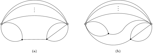
Refer to caption
Figure 2: Topologies of leading planar contributions.

The couplings in the ${\mathscr{N}}$=4 lagrangian which are relevant for these diagrams are

$${\mathscr{L}}_{\rm int}=\frac{1}{g_{{}_{\rm YM}}^{2}}\,{\rm Tr}\left(Z\left[\bar{\psi}^{-\,2}_{\dot{\alpha}},\bar{\psi}^{-\,{\dot{\alpha}}3}\right]+\left[Z,\varphi^{i}\right]\left[{\bar{Z}},\varphi^{i}\right]\right)\,.$$ (5.8)

We shall not compute explicitly the diagrams in figure 2. The sum of the two types of contributions is logarithmically divergent. For simplicity, in the following we shall only discuss the combinatorics associated with diagrams of the topology (a) in figure 2. Our considerations apply to the diagrams of type (b) as well and it is understood that the two types of contributions are included in the calculation of the two-point function.

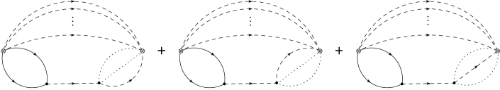
The planar diagrams in figure 2 require $p=0$ in the operator ${\mathscr{O}}_{1}$ (i.e. no $Z$ lines can be present between the two fermions) and $q=0$ or $q=1$ in the operator $\bar{\mathscr{O}}_{2}$ (there can be at most one ${\bar{Z}}$ between the two scalars in the trace). Indicating with dashed lines the $\langle Z{\bar{Z}}\rangle$ propagators, with dotted lines the $\langle\varphi\varphi\rangle$ propagators and with plain lines the fermion propagators, the relevant diagrams are those in figure 3. The first two diagrams involve the $q=0$ term in the operator $\bar{\mathscr{O}}_{2}$, whereas the third diagram involves the $q=1$ term.

Refer to caption
Figure 3: Planar diagrams of type (a).

Taking into account the normalisation of the operators the sum of the diagrams in figure 3 and the analogous ones obtained from (b) in figure 2 gives

$\displaystyle\frac{1}{\sqrt{J\left(\frac{g_{{}_{\rm YM}}^{2}N}{8\pi^{2}}\right)^{J+2}}}\,\frac{1}{\sqrt{J\left(\frac{g_{{}_{\rm YM}}^{2}N}{8\pi^{2}}\right)^{J+3}}}\,\frac{1}{g_{{}_{\rm YM}}^{4}}\,g_{{}_{\rm YM}}^{2(J+6)}\,N^{J+4}\left(1-{\rm e}^{-2\pi in/J}\right)f(x_{1},x_{2})$
$\displaystyle\sim\frac{(2\pi in)\,g_{{}_{\rm YM}}^{3}N^{3/2}}{J^{2}}\,f(x_{1},x_{2})=\frac{1}{J^{1/2}}\,(2\pi in)\,\left(\lambda^{\prime}\right)^{3/2}\,f(x_{1},x_{2})\,,$ (5.9)

where the logarithmically divergent function $f(x_{1},x_{2})$ is determined integrating over the position of the interaction points. In (5.9) the power of $g_{{}_{\rm YM}}$ results from the combination of two interaction vertices, $J+6$ propagators and the normalisation of the operators. The power of $N$ in the numerator in the first line comes from the colour contractions. The factor

$$\left(1-{\rm e}^{-2\pi in/J}\right)$$ (5.10)

comes from the sum of the three diagrams in figure 3. The first two diagrams give the 1 (no exponential because they correspond to $q=0$ in $\bar{\mathscr{O}}_{2}$) and the third diagram gives the exponential term. It has weight 2 and a relative minus sign with respect to the first two diagrams. Expanding (5.10) for large $J$ gives the result in (5.9), which vanishes in the BMN limit. Therefore the leading planar perturbative contributions vanish as expected.

Let us now consider the leading non-planar corrections to the two-point function (5.7). These correspond to string loop corrections to the dual amplitude which are expected to be non-zero in the plane-wave background. The leading non-planar corrections in the gauge theory are suppressed by a factor of $1/N^{2}$ with respect to the planar contributions. In order for the non-planar corrections to survive in the BMN limit additional powers of $J$ should arise. There are two sources of powers of $J$ in Feynman diagrams: the sums in the definitions of the operators and the number of diagrams at each genus. The operators (5.5)-(5.6) involve one sum each, so that potentially the sums can give a factor of $J^{2}$. This, however, requires that the sums be independent and the exponential factors in the operators be cancelled. It is easy to verify that this is never the case. For operators containing $J$ elementary fields the number of diagrams at genus $g$ grows as $J^{2g}$, so that again at the level of the leading non-planar corrections one can potentially get a factor of $J^{2}$ adding diagrams which give an equal contribution. This is what happens in the case of the two-point function (5.7). The relevant set of non-planar diagrams is depicted in figure 4. A similar set of diagrams is obtained from (b) in figure 2. The number of diagrams in these series grows as $J^{2}$.

Refer to caption
Figure 4: Non-planar contributions surviving in the BMN limit.

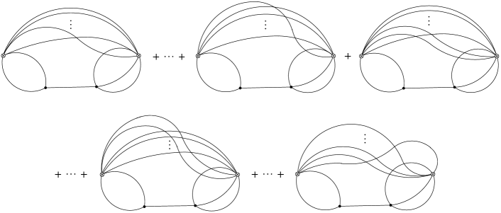
There are three sets of diagrams with the topologies in figure 4. The three sets can be obtained as non-planar deformations of the three diagrams in figure 3. Corresponding diagrams in the three series differ in the number of ${\bar{Z}}$ lines between the two $\varphi^{i}$ impurities in the operator $\bar{\mathscr{O}}_{2}$, i.e. they involve different terms in the sum in (5.6). This implies that adding up the three sets does not generate a factor such as (5.10) which would give a $1/J$ suppression as in (5.9).

In the case of the series obtained deforming the second diagram in figure 3 all the diagrams correspond to $q=0$ in the operator $\bar{\mathscr{O}}_{2}$, whereas in the other two series the diagrams have ${\bar{Z}}$ lines originating between the two $\varphi^{i}$ lines and thus correspond to different values of $q$. The leading large-$N$ contribution from the sum of the three series corresponding to the diagrams in figure 4 and the analogous ones obtained from (b) in figure 2 is

$\displaystyle\frac{1}{\sqrt{J\left(\frac{g_{{}_{\rm YM}}^{2}N}{8\pi^{2}}\right)^{J+2}}}\,\frac{1}{\sqrt{J\left(\frac{g_{{}_{\rm YM}}^{2}N}{8\pi^{2}}\right)^{J+3}}}\,\frac{1}{g_{{}_{\rm YM}}^{4}}g_{{}_{\rm YM}}^{2(J+6)}N^{J+2}$
$\displaystyle\times\sum_{k=0}^{J}\,(J-k)\left(1-2\,{\rm e}^{-2\pi i(k+1)n/J}+{\rm e}^{-2\pi ikn/J}\right)f(x_{1},x_{2})$
$\displaystyle\sim\frac{g_{{}_{\rm YM}}^{3}\,J}{N^{1/2}}\,\left(\frac{1}{2}+\frac{i}{2n\pi}\right)\,f(x_{1},x_{2})=\left(\frac{1}{2}+\frac{i}{2n\pi}\right)\left(g_{2}\right)^{2}\left(\lambda^{\prime}\right)^{3/2}\,f(x_{1},x_{2})\,,$ (5.11)

where we have used

$$\sum_{k=0}^{J}\,(J-k)\left(1-2\,{\rm e}^{-2\pi i(k+1)n/J}+{\rm e}^{-2\pi ikn/J}\right)\sim J^{2}\left(\frac{1}{2}+\frac{i}{2n\pi}\right)$$ (5.12)

in the large $J$ limit.

Therefore the two-point function (5.7) receives a non-vanishing contribution at the leading non-planar level in the BMN limit. The induced contribution to the matrix of anomalous dimensions is of order $(g_{2})^{2}\,(\lambda^{\prime})^{3/2}$.

Elements of the matrix of anomalous dimensions corresponding to non-real operators, such as those that we have considered, are in general complex. This is the case for the contribution extracted from the coefficient in (5.11) as well as for the vanishing planar contribution (5.9). The matrix element corresponding to the conjugate operators is the complex conjugate of the one computed here, so that the resulting matrix is hermitian and has real eigenvalues corresponding to the physical scaling dimensions of the operators. Notice also that, although half-integer powers of $\lambda^{\prime}$ appear in two-point functions mixing operators with fermionic and bosonic impurities, the anomalous dimensions obtained resolving the mixing have an expansion in integer powers of $\lambda^{\prime}$.

In this section we have presented a qualitative analysis of the leading perturbative contributions to a two-point function with mixing of the ${\rm NS}\!\otimes\!{\rm NS}$ and ${\rm R}\!\otimes\!{\rm R}$ sectors. Similar considerations can be repeated for the string amplitudes of the type described in section 4.2 and the dual gauge theory correlation functions of section 3.2. String amplitudes of the form (4.2)-(4.5) with $k\neq k^{\prime}$ and $h\neq h^{\prime}$ vanish at tree level, but are expected to receive a non-zero contribution at one loop. Therefore the dual two-point functions (3.12) should have the same behaviour as the mixed ones, i.e. they should vanish in the planar approximation at all orders in $\lambda^{\prime}$, but they should receive non-vanishing corrections beyond the zeroth order in $g_{2}$.

Acknowledgments.
AS acknowledges financial support from PPARC and Gonville and Caius college, Cambridge. We also wish to acknowledge support from the European Union Marie Curie Superstrings Network MRTN-CT-2004-512194.

References