hep-th/0512194

IPPP/06/07

DCPT/06/14

We study perturbative amplitudes in a large class of theories obtained by marginal deformations of the ${\cal N}=4$ supersymmetric Yang-Mills. We find that planar amplitudes in the deformed theories are closely related to planar amplitudes in the original ${\cal N}=4$ SYM. For some classes of deformations the amplitudes essentially coincide with the ${\cal N}=4$ amplitudes to all orders in planar perturbation theory. For more general classes of marginal deformations, the equivalence holds at up to four loops, and at five loops it is likely to break down. This implies that the iterative structure of planar MHV amplitudes recently discovered by Bern, Dixon and Smirnov in [1] for the ${\cal N}=4$ theory also manifests itself in a wider class of theories.

1 Introduction

The last two years have seen a remarkable progress in developing new conceptual and calculational approaches to compute perturbative on-shell scattering amplitudes in gauge theory. Witten has proposed a duality between the maximally supersymmetric ${\cal N}=4$ Yang-Mills theory and a twistor string theory [2]. This has stimulated wide-ranging progress in investigating scattering amplitudes in gauge theory at tree level and one-loop level, ranging from QCD to the ${\cal N}=4$ supersymmetric Yang-Mills, and using novel manifestly on-shell approaches – the MHV rules $+$ generalized unitarity [3, 4], and the on-shell recursion relations [5, 6]. For a summary of recent results one can consult on-line talks in [7].

One of the exciting recent developments is the remarkable proposal of Bern, Dixon and Smirnov [1] which applies to amplitudes in the ${\cal N}=4$ superconformal Yang-Mills theory. This proposal results in the formula which determines the structure of all $n$-point planar MHV amplitudes to all orders in perturbation theory. It follows that planar MHV amplitudes in the superconformal ${\cal N}=4$ Yang-Mills have an iterative structure, such that the kinematic dependence of all higher-loop MHV amplitudes can be determined from the known one-loop results. The main motivation of the present paper is to study how this result can be carried over to a wider family of gauge theories obtained by deformations of the ${\cal N}=4$ Yang-Mills. We will be mostly interested in the marginal deformations of the ${\cal N}=4$ studied earlier in [8, 9, 10] and we will also mention some known results [11] about orbifolds and orientifolds.

The proposal made in [1] gives an exponentiated ansatz which predicts the finite part of $n$-point planar MHV amplitudes in the superconformal ${\cal N}=4$ Yang-Mills to all orders in planar perturbation theory. The form of this ansatz is largely dictated by explicit three-loop calculations of four-point amplitudes carried out in [1], and is also based on earlier work [12, 13, 14, 15]. Importantly, it is also consistent with known results about exponentiation of IR divergencies [16, 17, 18] in a generic massless gauge theory.

${\cal N}=4$ SYM in the conformal phase is in many respects a special theory: as a field theory it is maximally supersymmetric, conformal and $SL(2,Z)$ self-dual. It also has a dual string theory description [19, 20] provided by the AdS/CFT correspondence. From the perspective of the on-shell amplitudes it is not clear at present which of these features (if any) are responsible for the iterative structure uncovered in [1]. This makes it particularly interesting to investigate the amplitudes in theories related to the ${\cal N}=4$ SYM but with lower degree of symmetry.

There are at least two distinct ways of deforming the ${\cal N}=4$ superconformal Yang-Mills theory to obtain another gauge theory with a lower degree of (super)-symmetry. One class of interesting deformations is the orbifold projection [11] of the ${\cal N}=4$ SYM. Orbifolding involves imposing a discrete projection operator on the parent ${\cal N}=4$ theory. This procedure modifies the field content of the theory: only the fields which are invariant under a discrete symmetry subgroup of the original theory are retained and other fields are projected out. Deformations of the ${\cal N}=4$ SYM by orbifolding reduces the amount of supersymmetry in the daughter theory to ${\cal N}=2$, ${\cal N}=1$ or ${\cal N}=0$. Remarkably, it was shown in [11] that in the large $N$ limit the parent and the daughter theories are perturbatively equivalent. This implies that planar perturbative amplitudes in the orbifold projections of ${\cal N}=4$ have exactly the same iterative structure as the one uncovered in [1] for ${\cal N}=4$.

Another method is to deform the ${\cal N}=4$ SYM by orientifolding [22]. The resulting orientifold daughter theory is a non-supersymmetric Yang-Mills with the $SU(N)$ gauge field plus 6 adjoint scalars and 4 Dirac fermions transforming in the (anti)symmetric representation. This theory is conformal at large $N$ and the planar equivalence with the ${\cal N}=4$ SYM is expected to hold in this case also non-perturbatively.

The second (and more non-trivial) way of modifying ${\cal N}=4$ is to deform it by adding marginal deformations [8, 9] to the Lagrangian. This leads to a conformally invariant theory with a lower ${\cal N}=1$ supersymmetry. The marginal deformations provide a much richer structure of deformed theories compared to orbifold projections. There is now a continuous family of deformations and the original ${\cal N}=4$ SYM corresponds a point on the moduli space of the deformed theories [8]. In this paper we will investigate relations between planar perturbative amplitudes in the ${\cal N}=4$ and in its marginal deformations. For related perturbative calculations of off-shell correlators in $\beta$-deformed theories see [23, 24, 25].

The paper is organized as follows. In Section 2 we collect some known facts about the ${\cal N}=4$ supersymmetric Yang-Mills and its marginal $\beta$-deformations. In Section 3 we discuss a special class of such deformations, which is characterized by a real deformation parameter $\beta=\beta_{\scriptscriptstyle R}.$ In the large $N$ limit these $\beta_{\scriptscriptstyle R}$-deformations form a one-real-parameter family of ${\cal N}=1$ conformal gauge theories. We prove that all planar amplitudes in these theories are equal to the corresponding amplitudes in the original ${\cal N}=4$ theory (times an overall phase factor which we determine). The proof holds to all orders in planar perturbation theory and applies to all amplitudes (MHV and non-MHV and for any number of external legs). This implies that the iterative structure of ${\cal N}=4$ amplitudes [1] is carried over to the family of theories deformed by $\beta_{\scriptscriptstyle R}$. Section 3.1 first illustrates how this proof works for some specific diagrams, and in Section 3.2 we give a more abstract general proof of the planar equivalence using star-products.

In Section 4 we consider more general marginal deformations with deformation parameters being complex. We show that all planar amplitudes in the deformed theory match those in the ${\cal N}=4$ SYM up to and including the four-loop level. At five loops, however, we find a mismatch which very likely will result in a breakdown in the iterative structure of planar amplitudes in the general deformed theory at five loops and beyond. We present our conclusions in Section 5.

2 Conformal deformations of ${\cal N}=4$ SYM

Our starting point is the ${\cal N}=4$ supersymmetric gauge theory. In terms of ${\cal N}=1$ superfields, the superpotential of the theory is

$$ig\,{\rm Tr}(\Phi_{1}\Phi_{2}\Phi_{3}-\Phi_{1}\Phi_{3}\Phi_{2})$$ (2.1)

Here $\Phi$’s are three chiral superfields transforming in the adjoint representation of the gauge group. In components, the ${\cal N}=4$ Lagrangian reads:

$${\cal{L}}={\cal{L}}_{b}+{\cal{L}}_{f}$$ (2.2)

where

$${\cal{L}}_{b}={\rm Tr}\left({1\over 4}F^{\mu\nu}F_{\mu\nu}+(D^{\mu}\bar{\Phi}^{i})(D_{\mu}\Phi_{i})-{g^{2}\over 2}[\Phi_{i},\Phi_{j}][\bar{\Phi}^{i},\bar{\Phi}^{j}]+{g^{2}\over 4}[\Phi_{i},\bar{\Phi}^{i}][\Phi_{j},\bar{\Phi}^{j}]\right)$$ (2.3)

and

$${\cal{L}}_{f}={\rm Tr}\left(\lambda_{A}\sigma^{\mu}D_{\mu}\bar{\lambda}^{A}-ig([\lambda_{4},\lambda_{i}]\bar{\Phi}^{i}+[\bar{\lambda}^{4},\bar{\lambda}^{i}]\Phi_{i})+{ig\over 2}(\epsilon^{ijk}[\lambda_{i},\lambda_{j}]\Phi_{k}+\epsilon_{ijk}[\bar{\lambda}^{i},\bar{\lambda}^{j}]\bar{\Phi}^{k})\right)$$

We use $A=1,\ldots,4$ and $i,j,k=1,\ldots,3$, such that $\Phi_{i}$ are the three complex scalar field components of the chiral superfields $\Phi_{i}$, and $\lambda_{i}$ are their fermionic superpartners. The fourth fermion $\lambda_{4}$ is the superpartner of the gluon. The $SU(N)$ generators are normalised as ${\rm Tr}\left(T^{a}T^{b}\right)=\delta^{ab}.$

We now turn to discuss marginal deformations of this theory. There is a 3-complex-parameter family of such deformations which preserve ${\cal N}=1$ supersymmetry [8]. These deformations are described [9], [8] by replacing (2.1) with the superpotential

$$ih\,{\rm Tr}(e^{i\pi\beta}\Phi_{1}\Phi_{2}\Phi_{3}-e^{-i\pi\beta}\Phi_{1}\Phi_{3}\Phi_{2})+ih^{\prime}\,{\rm Tr}(\Phi_{1}^{3}+\Phi_{2}^{3}+\Phi_{3}^{3})$$ (2.5)

At the classical level the deformations are marginal (since all operators in the component Lagrangian have classical mass dimension four) and the deformed theory is parameterized by four complex constants, $h,h^{\prime},\beta,\tau,$ with $\tau$ being the usual complexified gauge coupling. At the quantum level, this deformation is not exactly marginal since the operators in (2.5) can develop anomalous dimensions. Using constraints of ${\cal N}=1$ supersymmetry, and the exact NSVZ beta function approach [26], Leigh and Strassler [8] made an important observation. They showed that the deformation (2.5) is marginal at the quantum level subject to a single complex constraint on the four parameters, $\gamma(h,h^{\prime},\beta,\tau)=0.$ Here the function $\gamma$ is the sum of the anomalous dimensions $\gamma_{i}$ of the three fields $\Phi_{i}$, so that $\gamma=\sum_{i=1,2,3}\gamma_{i}.$ This constraint implies that there is a 3-complex-dimensional surface $\gamma(h,h^{\prime},\beta,\tau)=0$ of conformally invariant ${\cal N}=1$ theories obtained by deforming ${\cal N}=4$ SYM.

In this paper we set $h^{\prime}=0.$ In this case, the deformed theory preserves a global $U(1)\times U(1)$ symmetry,

$$U(1)_{1}: (\Phi_{1},\Phi_{2},\Phi_{3})\to(\Phi_{1},e^{i\varphi_{1}}\Phi_{2},e^{-i\varphi_{1}}\Phi_{3})$$

$$U(1)_{2}: (\Phi_{1},\Phi_{2},\Phi_{3})\to(e^{-i\varphi_{2}}\Phi_{1},e^{i\varphi_{2}}\Phi_{2},\Phi_{3})$$ (2.6)

where $\Phi_{i}$ are chiral ${\cal N}=1$ superfields.

At present, the complete solution of the Leigh-Strassler constraint,

$$\gamma(h,\beta,\tau)=\,0$$ (2.7)

is unknown, i.e. the function $\gamma=\sum_{i=1}^{3}\gamma_{i}(h,h^{\prime},\beta,\tau)$ in (2.7) is unknown beyond the two-loop order in perturbation theory [9]. One approach, followed in [27], is to work to the leading order in perturbation theory in deformations, in which case $\gamma$ is known. This motivated the authors of [27] to expand the $e^{\pm i\pi\beta}$ factors in (2.5) and to work to the first order in all deformations. We will follow a slightly different approach which does not require to expand the $\beta$-dependent factors. We will discuss a fixed-order in $h$ and $g$ perturbative treatment of general conformal deformations in Section 4.

But first we consider in Section 3 a restricted class of deformations which will allow us to work to all-orders in perturbation theory.

3 Planar amplitudes in real-$\beta$ deformations

Here we restrict the general deformation (2.5) to the ‘phase-deformation’ previously considered also by Lunin and Maldacena in [10]. We set $h=g,$ $h^{\prime}=0$ and keep $\beta$ real, $\beta=\beta_{\scriptscriptstyle R}\in{\bf R}$. The deformation of the superpotential of the ${\cal N}=4$ theory then reads

$$ig\,{\rm Tr}(\Phi_{1}\Phi_{2}\Phi_{3}-\Phi_{1}\Phi_{3}\Phi_{2})\to ig\,{\rm Tr}(e^{i\pi\beta_{\scriptscriptstyle R}}\Phi_{1}\Phi_{2}\Phi_{3}-e^{-i\pi\beta_{\scriptscriptstyle R}}\Phi_{1}\Phi_{3}\Phi_{2})\ .$$ (3.1)

This superpotential preserves the ${\cal N}=1$ supersymmetry of the original ${\cal N}=4$ SYM and leads to a theory with a global $U(1)\times U(1)$ symmetry (2.6). Less obvious is the fact (first proven in Ref. [25]) that (3.1) describes an exactly marginal deformation of the theory in the limit of large number of colors. As a by-product of our general discussion of planar amplitudes, in Section 3.2 we will reproduce this result of [25] and show that the planar perturbation theory of the deformed model is conformal, and the corresponding Leigh-Strassler constraint is satisfied at leading order in the $N\to\infty$ limit.

The main goal of this Section is to analyze scattering amplitudes of the theory deformed via (3.1) to all orders in planar perturbation theory, (and to all orders in $\beta_{\scriptscriptstyle R}$) and specifically compare them to the corresponding amplitudes in the original ${\cal N}=4$ SYM.

Lunin and Maldacena pointed out [10] that the deformation of the superpotential (3.1) can be viewed as arising from a new definition of the products between all fields in the ${\cal N}=4$ Lagrangian,

$$f*g\equiv e^{i\pi\beta_{\scriptscriptstyle R}(Q_{1}^{f}Q_{2}^{g}-Q_{2}^{f}Q_{1}^{g})}fg$$ (3.2)

where $fg$ is an ordinary product and $(Q_{1}^{\rm field},Q_{2}^{\rm field})$ are the $U(1)_{1}\times U(1)_{2}$ charges of the fields ($f$ or $g$). The values of the charges for all fields are read from (2.6):

$$\Phi_{1}\,(\Phi_{1},\lambda_{1})\,:\,\,\,\, (Q_{1}\,,Q_{2})=(0\,,-1)$$ (3.3)

$$\Phi_{2}\,(\Phi_{2},\lambda_{2})\,:\,\,\,\, (Q_{1}\,,Q_{2})=(1\,,1)$$ (3.4)

$$\Phi_{3}\,(\Phi_{3},\lambda_{3})\,:\,\,\,\, (Q_{1}\,,Q_{2})=(-1\,,0)$$ (3.5)

$$V\,(A_{\mu},\lambda_{4})\,:\,\,\,\, (Q_{1}\,,Q_{2})=(0\,,0)$$ (3.6)

and for the conjugate fields ($\bar{\Phi}_{i}$ and $\bar{\lambda}_{i}$) the charges are opposite.

For example, to calculate the star-product of three fields, $\Phi_{1}*\Phi_{2}*\Phi_{3}$, we first find $\Phi_{2}*\Phi_{3}=e^{i\pi\beta_{\scriptscriptstyle R}(0+1)}\Phi_{2}\Phi_{3}$ using (3.3),(3.4),(3.2). Then $\Phi_{1}*\Phi_{2}*\Phi_{3}=\Phi_{1}*(\Phi_{2}\Phi_{3})e^{i\pi\beta_{\scriptscriptstyle R}}=\Phi_{1}\Phi_{2}\Phi_{3}e^{i\pi\beta_{\scriptscriptstyle R}}$ since the charges of the composite field $\Phi_{2}\Phi_{3}$ are $(Q_{1},Q_{2})=(0,1),$ and as such cannot contribute to the last product. This implies

$${\rm Tr}(\Phi_{1}*\Phi_{2}*\Phi_{3}-\Phi_{1}*\Phi_{3}*\Phi_{2})=\,{\rm Tr}(e^{i\pi\beta_{\scriptscriptstyle R}}\Phi_{1}\Phi_{2}\Phi_{3}-e^{-i\pi\beta_{\scriptscriptstyle R}}\Phi_{1}\Phi_{3}\Phi_{2})$$ (3.7)

and confirms that the deformation of the superpotential Eq. (3.1) is induced by the star-product (3.2).

With the star-product (3.2), the component Lagrangian of the $\beta_{\scriptscriptstyle R}$-deformed theory (3.1) immediately follows from (2.3),(2). Only the third term in (2.3) and the last two terms in (2) change, such that in total we have

$${\cal{L}}=\,{\rm Tr}\Bigg{(}{1\over 4}F^{\mu\nu}F_{\mu\nu}+(D^{\mu}\bar{\Phi}^{i})(D_{\mu}\Phi_{i})-{g^{2}\over 2}[\Phi_{i},\Phi_{j}]_{\beta_{ij}}[\bar{\Phi}^{i},\bar{\Phi}^{j}]_{\beta_{ij}}+{g^{2}\over 4}[\Phi_{i},\bar{\Phi}^{i}][\Phi_{j},\bar{\Phi}^{j}]$$

$$+\lambda_{A}\sigma^{\mu}D_{\mu}\bar{\lambda}^{A}-ig([\lambda_{4},\lambda_{i}]\bar{\Phi}^{i}+[\bar{\lambda}^{4},\bar{\lambda}^{i}]\Phi_{i})+{ig\over 2}(\epsilon^{ijk}[\lambda_{i},\lambda_{j}]_{\beta_{ij}}\Phi_{k}+\epsilon_{ijk}[\bar{\lambda}^{i},\bar{\lambda}^{j}]_{\beta_{ij}}\bar{\Phi}^{k})\Bigg{)}$$

(3.8)

Here we introduced the $\beta_{\scriptscriptstyle R}$-deformed commutator of fields which is simply

$$[f_{i},g_{j}]_{\beta_{ij}}:=\,e^{i\pi\beta_{ij}}\,f_{i}g_{j}-\,e^{-i\pi\beta_{ij}}\,g_{j}f_{i}\ .$$ (3.9)

and $\beta_{ij}$ is defined as

$$\beta_{ij}=-\beta_{ji}\,,\quad\beta_{12}=\,-\beta_{13}=\,\beta_{23}:=\,\beta_{\scriptscriptstyle R}\ .$$ (3.10)

It is now easy to see which of the Feynman vertices are affected by $\beta_{\scriptscriptstyle R}$. All $\beta_{\scriptscriptstyle R}$-dependent four-scalar interactions are contained in the term

$$[\Phi_{i},\Phi_{j}]_{\beta_{ij}}[\bar{\Phi}^{i},\bar{\Phi}^{j}]_{\beta_{ij}}=\,e^{i2\pi\beta_{ij}}\,\Phi_{i}\Phi_{j}\bar{\Phi}^{i}\bar{\Phi}^{j}+\,e^{-i2\pi\beta_{ij}}\,\Phi_{j}\Phi_{i}\bar{\Phi}^{j}\bar{\Phi}^{i}-\,\Phi_{i}\Phi_{j}\bar{\Phi}^{j}\bar{\Phi}^{i}-\,\Phi_{j}\Phi_{i}\bar{\Phi}^{i}\bar{\Phi}^{j}$$ (3.11)

The first and second terms on the right hand side give the color-ordered Feynman vertex depicted in the first diagram in Figure 1.

\psfrag{r}{\LARGE${\bar{\Phi}_{j}}$}\psfrag{j}{\LARGE${\bar{\lambda}_{j}}$}\psfrag{h}{\LARGE${\lambda_{i}}$}\psfrag{g}{\LARGE${\lambda_{j}}$}\psfrag{k}{\LARGE${\bar{\lambda}_{i}}$}\psfrag{A}{\LARGE${-g^{2}\times e^{2\pi i\beta_{ij}}}$}\psfrag{B}{\LARGE${ig\,\epsilon^{ijk}}\times e^{\pi i\beta_{ij}}$}\psfrag{C}{\LARGE${ig\,\epsilon^{ijk}}\times e^{\pi i\beta_{ij}}$}\psfrag{a}{\LARGE${\Phi_{i}}$}\psfrag{b}{\LARGE${\Phi_{j}}$}\psfrag{f}{\LARGE${\bar{\Phi}_{i}}$}\psfrag{c}{\LARGE${\Phi_{k}}$}\psfrag{d}{\LARGE${\bar{\Phi}_{k}}$}\includegraphics{fig1beta.eps}

Figure 1: All $\beta_{\scriptscriptstyle R}$-dependent Feynman vertices in color-ordered perturbation theory.

\psfrag{A}{\LARGE${{1\over 2}\,g^{2}}$}\psfrag{B}{\LARGE${{1\over 4}\,g^{2}}$}\psfrag{C}{\LARGE${{1\over 4}\,g^{2}}$}\psfrag{a}{\LARGE${\Phi_{i}}$}\psfrag{b}{\LARGE${\Phi_{j}}$}\psfrag{f}{\LARGE${\bar{\Phi}_{j}}$}\psfrag{r}{\LARGE${\bar{\Phi}_{i}}$}\includegraphics{fig2beta.eps}

Figure 2: $\beta_{\scriptscriptstyle R}$-independent $\phi^{4}$ color-ordered vertices.

The $\beta_{\scriptscriptstyle R}$-independent third and fourth terms in (3.11) contribute to the first diagram in Figure 2. The remaining four-scalar interactions in (3.8) are determined by $(1/2)[\Phi_{i},\bar{\Phi}^{i}][\Phi_{j},\bar{\Phi}^{j}],$ and do not depend on $\beta.$ All the $\beta_{\scriptscriptstyle R}$-independent $\phi^{4}$ interactions are given by the three color-ordered vertices in Figure 2.

The only remaining $\beta_{\scriptscriptstyle R}$-dependent interactions are the Yukawa interactions – the last terms on the right hand side of Eq. (3.8). They give color-ordered Feynman vertices depicted in the second and third diagrams in Figure 1.

3.1 Planar amplitudes

Employing Feynman rules derived above we can make the following statements about scattering amplitudes in the $\beta_{\scriptscriptstyle R}$-deformed theory.

1. Any Feynman vertex involving a gluon, $g,$ or a gluino, $\bar{\lambda}_{4},$ $\lambda_{4},$ is unmodified. These vertices plus the three scalar interactions in Figure 2 give the complete set of the $\beta_{\scriptscriptstyle R}$-independent vertices.

2. Three vertices in Figure 1 are the only vertices which depend on the deformation parameter $\beta_{\scriptscriptstyle R}$. For a Feynman diagram in the $\beta_{\scriptscriptstyle R}$-deformed theory to agree with the corresponding diagram in the ${\cal N}=4$ SYM, it should either not contain these three types of vertices, or the phases introduced by these vertices should mutually cancel. Note that the phase depends on the order of the fields in the color-ordered vertices, for example the vertex of the type $\lambda_{1}\lambda_{2}\Phi_{3}\sim e^{i\pi\beta_{12}}=e^{i\pi\beta_{\scriptscriptstyle R}}$ while the vertex $\lambda_{2}\lambda_{1}\Phi_{3}\sim e^{i\pi\beta_{21}}=e^{-i\pi\beta_{\scriptscriptstyle R}}$.

3. All tree-level amplitudes in the deformed theory coincide with the corresponding amplitudes in the ${\cal N}=4$ theory up to a multiplicative constant factor. This constant depends only on the particle types in the external lines, and not on the internal structure of the diagram.

4. Tree-level and one-loop amplitudes with only gluons on the external lines are trivially identical to those in ${\cal N}=4$. This also applies to amplitudes with external $g$’s, $\bar{\lambda}_{4}$’s, and $\lambda_{4}$’s.

5. Beyond one-loop, non-planar diagrams of the $\beta_{\scriptscriptstyle R}$-deformed theory in general can contain non-trivial phase factors which depend on the structure of internal lines of individual diagrams.

6. A key point which we will prove below is that the total phase factor associated with any given planar amplitude is entirely determined by the external lines and does not depend on topologies and types of internal (loop) interactions. In other words, any planar loop amplitude in the $\beta_{\scriptscriptstyle R}$-deformed theory is equal to the corresponding amplitude in the original ${\cal N}=4$ SYM times an overall external phase factor. In particular, this universal phase factor can be easily determined using star-products of external fields (as will be explained in Section 3.2), or it can also be read off the corresponding tree-level amplitude, if it is non-vanishing.

7. It also follows that MHV amplitudes to all orders in planar perturbation theory are proportional to the corresponding tree-level amplitudes. The $\beta_{\scriptscriptstyle R}$-dependence of these planar all-orders amplitudes is entirely contained in the tree-level amplitude prefactor.

We start by considering planar multi-loop amplitudes with only gluons and gluinos: $\bar{\lambda}_{4}$ and $\lambda_{4}$ on the external lines. From the comments above it follows that these amplitudes in the deformed theory should be the same as in the original ${\cal N}=4$.

To verify this statement we first consider such diagrams where the $\beta_{\scriptscriptstyle R}$-phases are carried only by the 4-scalar interactions – the first vertex in Figure 1. What distinguishes this vertex from the rest of 4-scalar vertices (of Figure 2) is that it is of the alternating $i-j-i-j$ type (compared to the consecutive $i-i-j-j$ structure of three vertices in Figure 2). This index structure of the four scalar vertices is illustrated in Figure 3. It follows that only the $\beta$-dependent first vertex in Figure 3 corresponds to intersecting index-lines. In this sense the $\beta_{\scriptscriptstyle R}$-dependent vertex is ‘non-planar’.

\psfrag{i}{\LARGE${i}$}\psfrag{j}{\LARGE${j}$}\includegraphics{fig3beta.eps}

Figure 3: Index-lines representation of the four scalar vertices. The first diagram represents the $\beta_{\scriptscriptstyle R}$-dependent first vertex in Figure 1. The remaining three diagrams correspond to the three vertices in Figure 2.

Since gluons cannot join together scalar fields of two different flavors, $i$ and $j,$ the first vertex can appear either an even number of times, or it must be accompanied by a non-planar crossing. In planar diagrams, we can form closed planar chains of $\phi^{4}$ interactions and discover that all the individual phases cancel each other leaving us with the ${\cal N}=4$ result.

Now we add diagrams with the $\beta_{\scriptscriptstyle R}$-dependent Yukawa interactions. It can be shown that all individual phases will precisely cancel each other for planar amplitudes with external gluons, leaving behind the ${\cal N}=4$ expression. Instead of verifying this result on a diagram-by-diagram basis, in the following section 3.2 we will prove it in general using properties of star-products. But it may be instructive to first illustrate this phase cancellation with a simple example. Consider a 2-loop planar diagram with external gluons depicted in Figure 4.

\psfrag{a}{\LARGE${g}$}\psfrag{A}{\LARGE${\bar{\Phi}_{3}}$}\psfrag{B}{\LARGE${\Phi_{3}}$}\psfrag{C}{\LARGE${\lambda_{1}}$}\psfrag{D}{\LARGE${\bar{\lambda}_{1}}$}\psfrag{E}{\LARGE${\lambda_{2}}$}\psfrag{F}{\LARGE${\bar{\lambda}_{2}}$}\includegraphics{figdbox.eps}

Figure 4: Example of a 2-loop diagram contributing to the four-gluon amplitude. Red dots denote two $betaR$-dependent Yukawa vertices. Their phases cancel and the total contribution is $\beta_{\scriptscriptstyle R}$-independent.

There are two deformed Yukawa vertices in this diagram. The top vertex is $\lambda_{1}\lambda_{2}\Phi_{3}\sim ge^{i\pi\beta_{12}}\sim ge^{i\pi\beta_{\scriptscriptstyle R}},$ and the bottom vertex is $\bar{\lambda}_{2}\bar{\lambda}_{1}\bar{\Phi}_{3}\sim ge^{i\pi\beta_{21}}\sim ge^{-i\pi\beta_{\scriptscriptstyle R}}.$ The two phase factors cancel each other and the diagram is $\beta_{\scriptscriptstyle R}$-independent, as advertised. Discussion of general diagrams is deferred to Section 3.2.

When external lines include fields from $\Phi_{i}$ supermultiplets, the phase-dependence will remain. Nevertheless, at planar level, this dependence can be completely fixed by the external lines configuration in the following way. For every n-point planar color-ordered amplitude $A_{n}$ write down a factor of ${\rm Tr}(F_{1}*F_{2}*\ldots*F_{3})$ where $F_{i}$ denote all external fields in $A_{n}$

$$A_{n}(F_{1},F_{2},\ldots,F_{n})\,:\qquad{\rm Tr}(F_{1}*F_{2}*\ldots*F_{n})=[{\rm phase}(\beta_{\scriptscriptstyle R})]\,\times\,{\rm Tr}(F_{1}F_{2}\ldots F_{n})$$ (3.12)

Then the $\beta_{\scriptscriptstyle R}$-phase of the amplitude is equal to the [phase$(\beta_{\scriptscriptstyle R})$] of this star-product (see Section 3.2).

To illustrate this, we consider first two simple MHV planar amplitudes with four scalars, $A_{4}(\Phi_{1},\Phi_{2},\bar{\Phi}_{1},\bar{\Phi}_{2})$ and $A_{4}(\Phi_{1},\Phi_{2},\bar{\Phi}_{2},\bar{\Phi}_{1}).$ The $\beta_{\scriptscriptstyle R}$-dependence of the first amplitude is determined via:

$${\rm Tr}(\Phi_{1}*\Phi_{2}*\bar{\Phi}_{1}*\bar{\Phi}_{2})=\,e^{2i\pi\beta_{\scriptscriptstyle R}}\,{\rm Tr}(\Phi_{1}\Phi_{2}\bar{\Phi}_{1}\bar{\Phi}_{2})$$ (3.13)

and of the second, via:

$${\rm Tr}(\Phi_{1}*\Phi_{2}*\bar{\Phi}_{2}*\bar{\Phi}_{1})=\,1\,{\rm Tr}(\Phi_{1}\Phi_{2}\bar{\Phi}_{2}\bar{\Phi}_{1})$$ (3.14)

Examples of diagrams contributing to these amplitudes are shown in Figure 5.

\psfrag{a}{\LARGE${\Phi_{1}}$}\psfrag{b}{\LARGE${\Phi_{2}}$}\psfrag{c}{\LARGE${\bar{\Phi}_{1}}$}\psfrag{d}{\LARGE${\bar{\Phi}_{2}}$}\psfrag{A}{\LARGE${\lambda_{2}}$}\psfrag{B}{\LARGE${\bar{\lambda}_{2}}$}\psfrag{C}{\LARGE${\bar{\lambda}_{4}}$}\psfrag{D}{\LARGE${\lambda_{4}}$}\psfrag{E}{\LARGE${\lambda_{1}}$}\psfrag{F}{\LARGE${\bar{\lambda}_{1}}$}\psfrag{G}{\LARGE${\bar{\lambda}_{3}}$}\psfrag{H}{\LARGE${\lambda_{3}}$}\includegraphics{figbox.eps}

Figure 5: Two examples of 1-loop contributions to MHV amplitudes with four external scalars. The amplitude on the left is $\beta$-dependent, $A_{4}(\Phi_{1},\Phi_{2},\bar{\Phi}_{1},\bar{\Phi}_{2})\sim e^{2i\pi\beta_{\scriptscriptstyle R}}$. In the second amplitude, $A_{4}(\Phi_{1},\Phi_{2},\bar{\Phi}_{2},\bar{\Phi}_{1})\sim 1,$ the phases cancel.

It is easy to see that both $\beta_{\scriptscriptstyle R}$-dependent Yukawa vertices contribute $e^{i\pi\beta_{\scriptscriptstyle R}}$ each for the first diagram, and $e^{i\pi\beta_{\scriptscriptstyle R}}$ times $e^{-i\pi\beta_{\scriptscriptstyle R}}$ for the second one. Hence, $A_{4}(\Phi_{1},\Phi_{2},\bar{\Phi}_{1},\bar{\Phi}_{2})\sim e^{2i\pi\beta_{\scriptscriptstyle R}}$ and $A_{4}(\Phi_{1},\Phi_{2},\bar{\Phi}_{2},\bar{\Phi}_{1})\sim 1,$ in agreement with Eqs. (3.13),(3.14).

We can further consider Next-to-MHV amplitudes with six scalars, depicted in Figure 6.

\psfrag{a}{\LARGE${\Phi_{1}}$}\psfrag{b}{\LARGE${\bar{\Phi}_{2}}$}\psfrag{c}{\LARGE${\Phi_{3}}$}\psfrag{d}{\LARGE${\bar{\Phi}_{1}}$}\psfrag{e}{\LARGE${\Phi_{2}}$}\psfrag{f}{\LARGE${\bar{\Phi}_{3}}$}\psfrag{A}{\LARGE${\lambda_{3}}$}\psfrag{B}{\LARGE${\bar{\lambda}_{3}}$}\psfrag{D}{\LARGE${\lambda_{1}}$}\psfrag{C}{\LARGE${\bar{\lambda}_{1}}$}\psfrag{E}{\LARGE${\lambda_{2}}$}\psfrag{F}{\LARGE${\bar{\lambda}_{2}}$}\psfrag{W}{\LARGE${\lambda_{4}}$}\psfrag{Z}{\LARGE${\bar{\lambda}_{4}}$}\includegraphics{fighexagon.eps}

Figure 6: Two examples of Next-to-MHV amplitudes with six external scalars. The amplitude on the left, $A(\Phi_{1},\bar{\Phi}_{2},\Phi_{3},\bar{\Phi}_{1},\Phi_{2},\bar{\Phi}_{3},)\sim e^{-6i\pi\beta_{\scriptscriptstyle R}}$, and the amplitude on the right, $A(\Phi_{1},\bar{\Phi}_{2},\bar{\Phi}_{3},\Phi_{1},\Phi_{2},\Phi_{3},)\sim e^{2i\pi\beta_{\scriptscriptstyle R}}.$

The phase-factors associated with each of these diagrams are again in complete agreement with the general rule Eq. (3.12).

3.2 All-orders proof based on star-products

In this section we present a proof of the assertion that the $\beta_{\scriptscriptstyle R}$-dependence of a planar amplitude, $A_{n}(F_{1},\ldots,F_{n}),$ is entirely determined by the configuration of external fields $F_{1},\ldots F_{n}$ via Eq. (3.12).

We will rely on the fact the real-$\beta_{\scriptscriptstyle R}$ deformation we are studying is equivalent to the deformation by the star-product Eq. (3.2). The fact that the loop structure of planar diagrams does not affect the total phase-factor induced by star-products, is a well-known result in quantum field theories formulated on noncommutative spaces, [28, 29, 30]. However, the noncommutative product (3.2) which leads to the $\beta_{\scriptscriptstyle R}$-deformed theory, is defined differently from the Moyal star-product used in noncommutativity hence the proofs of planar equivalence presented in [28, 29, 30] require a modification, which we now present.

Each color-ordered vertex in Feynman perturbation theory can be represented by the corresponding term in the classical Lagrangian, e.g. ${\rm Tr}(\Phi_{j}\Phi_{i}\bar{\Phi}_{i}\bar{\Phi}_{j}),$ or ${\rm Tr}(\lambda_{i}\lambda_{j}\Phi_{k}),$ or in general ${\rm Tr}(F_{1}F_{2}\ldots F_{n})$ where $n$ is 3 or 4. In the $\beta_{\scriptscriptstyle R}$-deformed theory, this expression involves star-products, ${\rm Tr}(F_{1}*F_{2}*\ldots*F_{n}).$ Any two vertices connected by a propagator at tree-level can be represented by a single effective vertex, as shown in Figure 7. By this we mean that the total phase factor of the connected tree diagram made out of these two vertices is equal to the phase factor of the effective vertex. Indeed, using the fact that each vertex $V$ in Figure 7 has a vanishing total $Q$-charge and the associativity of the star-product, we have

\psfrag{a}{\LARGE${F_{i}}$}\psfrag{b}{\LARGE${F_{j}}$}\psfrag{c}{\LARGE${F_{k}}$}\psfrag{d}{\LARGE${F_{l}}$}\psfrag{F}{\LARGE${F_{I}}$}\psfrag{B}{\LARGE${\bar{F}_{I}}$}\includegraphics{figstar1.eps}

Figure 7: At tree level all vertices can be joined together into an effective vertex without changing the total $\beta_{\scriptscriptstyle R}$-phase of the diagram. $F$’s denote generic component fields. We use the bar in $\bar{F}_{I}$ to emphasize that this field has opposite $Q$-charges to the $F_{I}$ field on the other end of the internal propagator.

$$V_{n}V_{m}\,=\,(F_{j}*\ldots*F_{i}*F_{I})\,(\bar{F}_{I}*F_{k}*\ldots*F_{l})$$ (3.15)

$$=\,(F_{j}*\ldots*F_{i}*F_{I})*(\bar{F}_{I}*F_{k}*\ldots*F_{l})\,=\,(F_{j}*\ldots*F_{i})*(F_{I}*\bar{F}_{I})*(F_{k}*\ldots*F_{l})$$

but since $F_{I}$ and $\bar{F}_{I}$ have opposite U(1) charges, we have $F_{I}*\bar{F}_{I}=\,1\,F_{I}\bar{F}_{I}\sim 1$ and this implies

$$V_{n}V_{m}\sim(F_{j}*\ldots*F_{i}*F_{k}*\ldots*F_{l})=V_{n+m-2}$$ (3.16)

Hence an arbitrary tree amplitude has a phase factor which can be read of the single effective vertex using the rule above. This verifies the statement in item (3) in the previous section.

Now we generalize to loops. Since a tree-level diagram can be reduced to an effective vertex, a loop diagram can be represented by such a vertex with self-contractions depicted in Figure 8. A planar loop diagram must contain no intersecting lines.

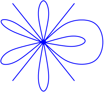
Figure 8: Reduced planar loop diagram is given by the corresponding effective tree-level vertex with self-contraction. Planarity implies that none of the (external and internal) lines can intersect. Reduced diagram has the same $\beta_{\scriptscriptstyle R}$-phase as the original Feynman diagram.

It is easy to see that each planar self-contraction can be removed without affecting the total $\beta_{\scriptscriptstyle R}$-dependence of the diagram. This is because at the both ends of the self-contraction we have fields of the opposite charges, and these fields are positioned next to each other due to planarity, $F_{I}*\bar{F}_{I}\sim 1.$ Hence the phase-dependence of each planar diagram can be read off an effective tree-level vertex in agreement with Eq. (3.12). This completes the proof.

We conclude that all planar amplitudes in the $\beta_{\scriptscriptstyle R}$-deformed theory are proportional to their ${\cal N}=4$ counterparts. Since, the ${\cal N}=4$ theory was finite, this implies the UV-finiteness (or conformal invariance) of the deformed theory in the planar limit.

It follows that the intriguing iterative structure of the planar MHV amplitudes in ${\cal N}=4$ superconformal Yang-Mills uncovered in Ref. [1] is carried over to the phase-deformed theory without modifications and to all orders in perturbation theory. For generic MHV planar amplitudes, the entire $\beta_{\scriptscriptstyle R}$-dependence is contained in the tree-level prefactor.

4 More general conformal deformations

We now consider more general deformations of ${\cal N}=4$ which do not require $\beta$ to be real.

4.1 A non-supersymmetric generalization

There is one simple class of extended deformations obtained by complexifying $\beta_{\scriptscriptstyle R}$ in the component Lagrangian (3.8). The deformation parameter is now a complex-valued $\beta$

$$\beta=\beta_{\scriptscriptstyle R}+i\chi\ ,\qquad\beta_{\scriptscriptstyle R}\ ,\ \chi\in{\bf R}$$ (4.1)

The Lagrangian takes the same form as in (3.8), but the $\beta$-deformed commutators (3.9) are written in terms of complex $\beta_{ij}$,

$$\beta_{12}=\,-\beta_{13}=\,\beta_{23}:=\,\beta\in{\bf C}\ ,\qquad\beta_{ij}=-\beta_{ji}$$ (4.2)

We note that this theory (which can also be obtained by complexifying the star-product of component fields) is non-supersymmetric and is different from the ${\cal N}=1$ supersymmetric deformations described by (2.5) with complex $\beta.$ All the results of Section 3 including precise cancellation of $\beta$ dependence in planar diagrams of gluons are carried over without modifications to this complexified family of deformations. Hence we conclude that there is a two-real-dimensional family of transformations of ${\cal N}=4$ which is nonsupersymmetric, but has exactly the same (up to an overall complexified phase factor) planar amplitudes as the ${\cal N}=4$ theory to all orders in perturbation theory.

This ‘planar equivalence’ of perturbative amplitudes in the non-supersymmetric deformation and in the ${\cal N}=4$ parent, however, should not be interpreted as the large-$N$ equivalence of the two theories. The arguments of Ref. [31] imply that generic non-supersymmetric $\beta$-deformed theories are not conformal and generate a scale due to couplings with double-trace operators. This means that perturbative vacuum is not a true vacuum of the theory, and the ‘planar equivalence’ in the non-supersymmetric case should be viewed only as a formal relation between perturbative amplitudes.

4.2 ${\cal N}=1$ supersymmetric $\beta$-deformations

The second class of more general deformations of ${\cal N}=4$ is described by the superpotential

$${\cal W}=\,ih\,{\rm Tr}(e^{i\pi\beta}\Phi_{1}\Phi_{2}\Phi_{3}-e^{-i\pi\beta}\Phi_{1}\Phi_{3}\Phi_{2})$$ (4.3)

Here $h$ and $\beta$ are complex parameters, and $\beta$ is given in (4.1). For a generic deformation (4.3) which preserves conformal invariance of the theory only at the classical level, it is pretty clear that the deformations will not cancel from planar diagrams – they are not simple phases after all. But there may exist a condition on the parameters $h$ and $\beta$ for which such cancellations do occur at least in the first few orders of perturbation theory. Can this condition be identical to the CFT constraint (2.7)?

The goal of this Section is to show that this is indeed the case, and that in the deformed theory all planar amplitudes with external gluons are equal to those in the ${\cal N}=4$ SYM up to a five-loop level. At five loops and beyond we expect that planar amplitudes in the two theories begin to differ.

The UV finiteness (or equivalently the conformal invariance) of the theory deformed by the superpotential

$${\cal W}\,=\,\frac{1}{3!}\,C^{ijk}_{abc}\,\Phi^{a}_{i}\Phi^{b}_{j}\Phi^{c}_{k}$$ (4.4)

is guaranteed if the following condition [9] is satisfied

$$C^{ijk}_{abc}\,C^{*\,dbc}_{\,\,\,ljk}\,=\,2g^{2}\,\delta^{i}_{l}\,\delta^{d}_{a}\,T_{R}$$ (4.5)

Here all $\Phi$’s transform in the adjoint representation and $T_{R}=N.$ The constraint (4.5) follows from the one-loop finiteness of the theory, but it also automatically guarantees the UV finiteness of the ${\cal N}=1$ theory at two-loop level [9]. Hence, (4.5) is the solution of the Leigh-Strassler CFT constraint (2.7) at the two-loop level.

Our superpotential (4.3), corresponds to

$$C^{123}_{abc}\,\sim\,-\,h\left(f^{abc}(e^{i\pi\beta}+e^{-i\pi\beta})+id^{abc}(e^{i\pi\beta}-e^{-i\pi\beta})\right)$$ (4.6)

and the two-loop CFT constraint (4.5) gives [23, 24]

$$|h|^{2}\left({\rm cosh}(2\pi\chi)+\frac{2}{N^{2}}{\rm cos}(2\pi\beta_{\scriptscriptstyle R})-\frac{2}{N^{2}}{\rm cosh}(2\pi\chi)\right)=\,g^{2}$$ (4.7)

In the planar approximation we neglect $1/N^{2}$ terms and the constraint simplifies,

$$|h|^{2}{\rm cosh}(2\pi\chi)=\,g^{2}$$ (4.8)

An important feature of the planar constraint (4.8) is that it does not depend on $\beta_{\scriptscriptstyle R}$ and, furthermore, for real $\beta$ it collapses to $|h|^{2}=g^{2}.$ This verifies at the two-loop level the fact that the real-$\beta_{\scriptscriptstyle R}$-deformation is an exactly marginal deformation in the planar limit – in agreement with the more powerful all-orders discussion given earlier in Section 3. As a bonus, we also see that subleading in $1/N^{2}$ terms in (4.7) (which do not affect planar diagrams) do in fact depend on $\beta_{\scriptscriptstyle R}$.

We are now ready to concentrate on the amplitudes with external gluons in planar perturbation theory, which is the main subject of this Section. These amplitudes can be organized in a simple way using supergraph Feynman perturbation theory. The relevant vertices are the trilinear ones arising from the superpotential ${\cal W}$ in (4.3) and its Hermitian conjugate ${\cal\bar{W}}$. These vertices and the superfield propagator are shown in Figure 9.

\psfrag{A}{\LARGE${\Phi_{1}}$}\psfrag{B}{\LARGE${\Phi_{2}}$}\psfrag{C}{\LARGE${\Phi_{3}}$}\psfrag{D}{\LARGE${\bar{\Phi}_{1}}$}\psfrag{G}{\LARGE${\bar{\Phi}_{2}}$}\psfrag{H}{\LARGE${\bar{\Phi}_{3}}$}\psfrag{W}{\LARGE${ih\,e^{i\pi\beta}}$}\psfrag{X}{\LARGE${-ih\,e^{-i\pi\beta}}$}\psfrag{Y}{\LARGE${ih^{*}\,e^{i\pi\beta^{*}}}$}\psfrag{Z}{\LARGE${-ih^{*}\,e^{-i\pi\beta^{*}}}$}\psfrag{E}{\LARGE${\Phi_{i}}$}\psfrag{F}{\LARGE${\bar{\Phi}_{i}}$}\includegraphics{figSVbeta.eps}

Figure 9: Supergraph Feynman rules for (anti)-chiral superfields corresponding to the superpotential in Eq. (4.3) and its conjugate. Arrows are outgoing for chiral $\Phi$ and incoming for anti-chiral $\bar{\Phi}$ superfields. The propagator connects chiral to anti-chiral superfields of the same flavor.

Our goal is to determine the dependence of planar multi-loop amplitudes on the coupling constant parameters $g$, $h$ and $\beta$ in the deformed theory and to try to match it with the $g$-dependence of the undeformed ${\cal N}=4$ amplitudes using the CFT constraint (4.8). To achieve this we do not need to consider interactions with the ${\cal N}=1$ vector multiplet, only the matter (anti)-chiral fields, $\Phi_{i}$, $\bar{\Phi}_{i}$, are relevant. This is because interactions with vectors depend only on the original coupling $g$ and not on the deformation parameters $\beta$ and $h$. Furthermore, gluons and gluinos $\lambda_{4}$ and $\bar{\lambda}_{4}$ do not change the flavor $i$ of matter superfields $\Phi_{i}$, $\bar{\Phi}_{i}$, hence they are irrelevant for the matching to ${\cal N}=4$.

Hence the relevant diagrams are the planar vacuum diagrams built solely from chiral $\Phi_{1,2,3}$ and anti-chiral $\bar{\Phi}_{1,2,3}$ matter superfields using super-Feynman rules of Figure 9. We will call them vacuum $\Phi$-diagrams. To reproduce the actual amplitude in the full theory, internal and external vector superfields are supposed to be added in all possible ways to these effective vacuum $\Phi$-diagrams. However, this would not affect the overall dependence on the deformation parameters $h$ and $\beta$.

The simplest vacuum $\Phi$-diagram with a non-trivial dependence on couplings occurs at the two-loop level and is shown in Figure 10.

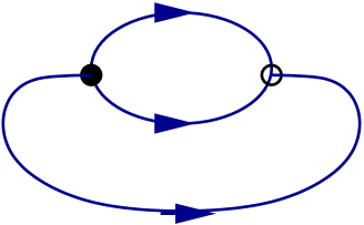
Figure 10: Planar vacuum $\Phi$-diagram at the two-loop level. After summing over all flavors in the loops the deformation parameters appear in the combination, $|h|^{2}{\rm cosh(2\pi\chi)}=g^{2}$ via Eq. (4.8). This matches with the ${\cal N}=4$ result.

After summing over all allowed flavors of $\Phi$ circulating in the loops, one easily finds that the total two-loop contribution is proportional to $|h|^{2}{\rm cosh(2\pi\chi)}.$ The CFT constraint (4.8) guarantees that this matches precisely with the two-loop result in the undeformed ${\cal N}=4$ theory.

This two-loop matching could have been easily anticipated. The dependence of the amplitude in Figure 10 on $h$ and $\beta$ is the same as in the one-loop $\Phi$-self-energy contributions shown in Figure 11.

\psfrag{A}{\LARGE${\Phi_{1}}$}\psfrag{B}{\LARGE${\Phi_{2}}$}\psfrag{C}{\LARGE${\Phi_{3}}$}\psfrag{D}{\LARGE${\bar{\Phi}_{1}}$}\psfrag{G}{\LARGE${\bar{\Phi}_{2}}$}\psfrag{H}{\LARGE${\bar{\Phi}_{3}}$}\psfrag{W}{\LARGE${|h|^{2}\,e^{-2\pi\chi}}$}\psfrag{X}{\LARGE${|h|^{2}\,e^{2\pi\chi}}$}\includegraphics{figSEbeta.eps}

Figure 11: Self-energy contributions at one loop involving deformed supergraph vertices. Total contribution of these two diagrams in the deformed theory is proportional to $2|h|^{2}{\rm cosh(2\pi\chi)}.$

The latter give rise to the one-loop anomalous dimension $\gamma$ of $\Phi$. The planar CFT constraint (4.8) arises from matching $\gamma$ in the deformed theory and to the ${\cal N}=4$ (where it vanishes). From Figure 11 we read the matching condition as $2|h|^{2}{\rm cosh}(2\pi\chi)=2g^{2}$ which is precisely Eq. (4.8).

From this analysis we conclude that we can drop all self-energy insertions into multi-loop planar vacuum $\Phi$-diagrams of the deformed theory – these insertions will always match with the ${\cal N}=4$ result. Hence, we will neglect diagrams which include bubbles as subdiagrams.

It is easy to see that one cannot form triangles using the Feynman rules in Figure 9. Indeed, each holomorphic in $\Phi$ vertex can be connected only to an anti-holomorphic one. A triangle would necessarily involve two adjacent vertices of the same type. Having lost triangles and bubbles we turn to boxes as building blocks. The first vacuum diagram involving boxes (with no self-energy contractions) occurs only at the five-loop level. It is depicted in figure 12.

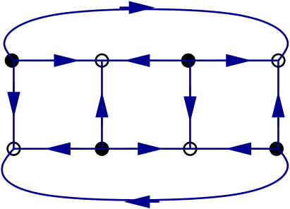
Figure 12: Planar vacuum $\Phi$-diagrams without bubbles at five-loop level are made of boxes.

Summing over all allowed flavors in the loops in Figure 12 we can find the total dependence of the five-loop contribution on the deformation parameters. There is an overall factor of $|h|^{8}$ but the dependence on $\chi$ is not of the form ${\rm cosh}^{4}(2\pi\chi)$. Hence the coupling constant dependence is not given simply by $g^{8}$ and this does not match with the five-loop amplitudes in the ${\cal N}=4$ theory.

One has to be a little more careful with this conclusion since the expression (4.8) is not an exact solution of the CFT constraint, and it does in general receive perturbative corrections. In perturbation theory we can treat of $g^{2}\sim|h|^{2}\ll 1$ and $\chi\sim 1$. Then we expect corrections on the right hand side of (4.8) suppressed by powers of $g$ or $h.$ One can in principle solve the corrected constraint in terms of $h$ order by order in $g$ and substitute this solution for $h$ into the bare superpotential (4.3). This would amount to fine-tuning the bare deformation order by order in $g$. It is this fine-tuned theory which has to be conformally invariant [9]. This fine-tuning is designed to force the anomalous dimensions and the beta-function vanish (thus removing UV-divergencies from planar amplitudes) via cancellations between diagrams with different numbers of loops. It is however unlikely that such cancellations can repair the $\chi$-dependence of the finite parts of the $n$-point amplitudes with external gluons.

5 Conclusions

We have shown that there is a planar equivalence between perturbative amplitudes in the ${\cal N}=4$ theory and its various deformations.

This equivalence is perturbatively exact (i) for theories obtained from ${\cal N}=4$ by orbifold projections [11]; (ii) for a one parameter family of marginal $\beta_{\scriptscriptstyle R}$ deformations considered in Section 3 and (iii) for complex non-supersymmetric deformations considered in Section 4.1. In all these cases, the remarkable iterative structure of planar MHV amplitudes proposed by Bern, Dixon and Smirnov for the ${\cal N}=4$ theory carries over without modifications.

For more general marginal deformations studied in Section 4 the planar equivalence holds for up to five loops where it (very likely) breaks down. This fact is intriguing for two reasons: one is that the planar equivalence with the ${\cal N}=4$ theory holds all the way to four loops. And second, is the fact that even the original ${\cal N}=4$ all-orders proposal of [1] was not checked explicitly beyond the three loop level.

Conformal invariance of the theory is likely to play a role in explaining the underlying principles behind the iterative structure of MHV amplitudes [1]. However on its own conformal invariance does not appear to be a sufficient reason for this behavior. It is tempting to speculate that the transformation properties of the deformed theories under the $SL(2,Z)$ as well as the AdS/CFT correspondence will also play a role.

Acknowledgements

I would like to thank Lance Dixon for conversations and comments which greatly improved this paper. I am grateful to Nigel Glover, Simon Badger and George Georgiou for many useful discussions about amplitudes and loops and to Adi Armoni for helpful comments about orientifolding ${\cal N}=4$ SYM.

References

- [1] Z. Bern, L. J. Dixon and V. A. Smirnov, Phys. Rev. D 72 (2005) 085001 [hep-th/0505205].
- [2] E. Witten, Commun. Math. Phys. 252 (2004) 189 [hep-th/0312171].
-
[3]
F. Cachazo, P. Svrcek and E. Witten,
JHEP 0409 (2004) 006 [hep-th/0403047]
G. Georgiou and V. V. Khoze, JHEP 05 (2004) 070 [hep-th/0404072]
C.-J. Zhu, JHEP 04 (2004) 032 [hep-th/0403115]
J.-B. Wu and C.-J. Zhu, JHEP 07 (2004) 032 [hep-th/0406085]
I. Bena, Z. Bern and D. A. Kosower, Phys. Rev. D71 (2005) 045008 [hep-th/0406133]
D. A. Kosower, Phys. Rev. D71 (2005) 045007 [hep-th/0406175]
G. Georgiou, E. W. N. Glover and V. V. Khoze, JHEP 07 (2004) 048 [hep-th/0407027]
L. J. Dixon, E. W. N. Glover and V. V. Khoze, JHEP 12 (2004) 015 [hep-th/0411092]
Z. Bern, D. Forde, D. A. Kosower and P. Mastrolia, hep-ph/0412167
S. D. Badger, E. W. N. Glover and V. V. Khoze, JHEP 0503, 023 (2005) [hep-th/0412275]
T. G. Birthwright, E. W. N. Glover, V. V. Khoze and P. Marquard, JHEP 0505 (2005) 013 [hep-ph/0503063]; JHEP 0507 (2005) 068 [hep-ph/0505219]
K. Risager, hep-th/0508206
P. Mansfield, hep-th/0511264. -
[4]
F. Cachazo, P. Svrcek and E. Witten,
JHEP 0410 (2004) 074
[hep-th/0406177]
JHEP 0410 (2004) 077 [hep-th/0409245]
A. Brandhuber, B. J. Spence and G. Travaglini, Nucl. Phys. B 706 (2005) 150 [arXiv:hep-th/0407214]
F. Cachazo, hep-th/0410077
R. Britto, F. Cachazo and B. Feng, Phys. Rev. D 71 (2005) 025012 [hep-th/0410179]
Z. Bern, V. Del Duca, L. J. Dixon and D. A. Kosower, Phys. Rev. D 71 (2005) 045006 [hep-th/0410224]
C. Quigley and M. Rozali, JHEP 0501 (2005) 053 [hep-th/0410278]
J. Bedford, A. Brandhuber, B. J. Spence and G. Travaglini, Nucl. Phys. B 706 (2005) 100 [hep-th/0410280]
S. J. Bidder, N. E. J. Bjerrum-Bohr, L. J. Dixon and D. C. Dunbar, Phys. Lett. B 606 (2005) 189 [hep-th/0410296]
R. Britto, F. Cachazo and B. Feng, Nucl. Phys. B 725 (2005) 275 [hep-th/0412103]
J. Bedford, A. Brandhuber, B. J. Spence and G. Travaglini, Nucl. Phys. B 712 (2005) 59 [hep-th/0412108]
Z. Bern, L. J. Dixon and D. A. Kosower, Phys. Rev. D 72 (2005) 045014 [hep-th/0412210]
S. J. Bidder, N. E. J. Bjerrum-Bohr, D. C. Dunbar and W. B. Perkins, Phys. Lett. B 612 (2005) 75 [hep-th/0502028]
R. Britto, E. Buchbinder, F. Cachazo and B. Feng, Phys. Rev. D 72 (2005) 065012 [hep-ph/0503132]
R. Britto, B. Feng, R. Roiban, M. Spradlin and A. Volovich, Phys. Rev. D 71 (2005) 105017 [hep-th/0503198]
S. J. Bidder, D. C. Dunbar and W. B. Perkins, JHEP 0508 (2005) 055 [hep-th/0505249]
A. Brandhuber, S. McNamara, B. J. Spence and G. Travaglini, JHEP 0510 (2005) 011 [hep-th/0506068]
E. I. Buchbinder and F. Cachazo, JHEP 0511 (2005) 036 [arXiv:hep-th/0506126]
A. Brandhuber, B. Spence and G. Travaglini, hep-th/0510253. -
[5]
R. Britto, F. Cachazo and B. Feng,
Nucl. Phys. B 715 (2005) 499
[hep-th/0412308]
R. Roiban, M. Spradlin and A. Volovich, Phys. Rev. Lett. 94, 102002 (2005) [hep-th/0412265]
R. Britto, F. Cachazo, B. Feng and E. Witten, Phys. Rev. Lett. 94 (2005) 181602 [hep-th/0501052]
M. x. Luo and C. k. Wen, JHEP 0503 (2005) 004 [hep-th/0501121]; Phys. Rev. D 71 (2005) 091501 [hep-th/0502009]
S. D. Badger, E. W. N. Glover, V. V. Khoze and P. Svrcek, JHEP 0507 (2005) 025 [hep-th/0504159]
S. D. Badger, E. W. N. Glover and V. V. Khoze, [hep-th/0507161]. -
[6]
Z. Bern, L. J. Dixon and D. A. Kosower,
Phys. Rev. D 71 (2005) 105013
[hep-th/0501240];
Phys. Rev. D 72 (2005) 125003
[hep-ph/0505055];
hep-ph/0507005
Z. Bern, N. E. J. Bjerrum-Bohr, D. C. Dunbar and H. Ita, hep-ph/0507019. - [7] From Twistors to Amplitudes, QMUL Workshop, 3-5 November 2005, on-line talks at http://www.strings.ph.qmul.ac.uk/%7Eandreas/FTTA/program.htm
- [8] R. G. Leigh and M. J. Strassler, Nucl. Phys. B 447, 95 (1995) [hep-th/9503121].
-
[9]
A. Parkes and P. C. West,
Phys. Lett. B 138, 99 (1984)
P. C. West, Phys. Lett. B 137, 371 (1984)
D. R. T. Jones and L. Mezincescu, Phys. Lett. B 138, 293 (1984)
S. Hamidi, J. Patera and J. H. Schwarz, Phys. Lett. B 141, 349 (1984)
W. Lucha and H. Neufeld, Phys. Lett. B 174, 186 (1986)
D. R. T. Jones, Nucl. Phys. B 277, 153 (1986)
X. d. Jiang and X. J. Zhou, Commun. Theor. Phys. 5, 179 (1986); Phys. Rev. D 42, 2109 (1990)
A. V. Ermushev, D. I. Kazakov and O. V. Tarasov, Nucl. Phys. B 281, 72 (1987)
D. I. Kazakov, Mod. Phys. Lett. A 2, 663 (1987). - [10] O. Lunin and J. Maldacena, JHEP 0505 (2005) 033 [hep-th/0502086].
-
[11]
M. Bershadsky, Z. Kakushadze and C. Vafa,
Nucl. Phys. B 523 (1998) 59
[hep-th/9803076]
M. Bershadsky and A. Johansen, Nucl. Phys. B 536 (1998) 141 hep-th/9803249]. - [12] Z. Bern, L. J. Dixon, D. C. Dunbar and D. A. Kosower, Nucl. Phys. B 425 (1994) 217 [hep-ph/9403226]; Nucl. Phys. B 435 (1995) 59 [hep-ph/9409265].
-
[13]
Z. Bern, J. S. Rozowsky and B. Yan,
Phys. Lett. B 401 (1997) 273
[hep-ph/9702424]
Z. Bern, L. J. Dixon, D. C. Dunbar, M. Perelstein and J. S. Rozowsky, Nucl. Phys. B 530 (1998) 401 [hep-th/9802162]. - [14] C. Anastasiou, Z. Bern, L. J. Dixon and D. A. Kosower, Phys. Rev. Lett. 91 (2003) 251602 [hep-th/0309040]; [hep-th/0402053].
- [15] V. A. Smirnov, Phys. Lett. B 567 (2003) 193 [hep-ph/0305142].
- [16] G. Sterman and M. E. Tejeda-Yeomans, Phys. Lett. B 552 (2003) 48 [hep-ph/0210130].
- [17] L. Magnea and G. Sterman, Phys. Rev. D 42 (1990) 4222.
- [18] S. Catani, Phys. Lett. B 427 (1998) 161 [hep-ph/9802439].
-
[19]
J. M. Maldacena,
Adv. Theor. Math. Phys. 2 (1998) 231
[Int. J. Theor. Phys. 38 (1999) 1113]
[hep-th/9711200]
S. S. Gubser, I. R. Klebanov and A. M. Polyakov, Phys. Lett. B 428 (1998) 105 [hep-th/9802109]
E. Witten, Adv. Theor. Math. Phys. 2 (1998) 253 [hep-th/9802150]. -
[20]
D. Berenstein, J. M. Maldacena and H. Nastase,
JHEP 0204 (2002) 013
[hep-th/0202021]
S. S. Gubser, I. R. Klebanov and A. M. Polyakov, Nucl. Phys. B 636 (2002) 99 [hep-th/0204051]. -
[21]
M. J. Strassler,
[hep-th/0104032]
D. Tong, JHEP 0303 (2003) 022 [hep-th/0212235]
P. Kovtun, M. Unsal and L. G. Yaffe, JHEP 0312 (2003) 034 [hep-th/0311098]. - [22] A. Armoni, M. Shifman and G. Veneziano, Nucl. Phys. B 667 (2003) 170 [hep-th/0302163]; [hep-th/0403071].
- [23] D. Z. Freedman and U. Gursoy, JHEP 0511 (2005) 042 [hep-th/0506128].
- [24] S. Penati, A. Santambrogio and D. Zanon, JHEP 0510 (2005) 023 [hep-th/0506150].
- [25] A. Mauri, S. Penati, A. Santambrogio and D. Zanon, JHEP 0511 (2005) 024 [hep-th/0507282].
-
[26]
V. A. Novikov, M. A. Shifman, A. I. Vainshtein and V. I. Zakharov,
Phys. Lett. B 166 (1986) 329;
M. A. Shifman and A. I. Vainshtein, Nucl. Phys. B 277 (1986) 456; Nucl. Phys. B 359 (1991) 571. - [27] M. Kulaxizi and K. Zoubos, [hep-th/0410122].
- [28] T. Filk, Phys. Lett. B 376 (1996) 53.
- [29] N. Ishibashi, S. Iso, H. Kawai and Y. Kitazawa, Nucl. Phys. B 573 (2000) 573 [hep-th/9910004].
- [30] S. Minwalla, M. Van Raamsdonk and N. Seiberg, JHEP 0002 (2000) 020 [hep-th/9912072].
- [31] A. Dymarsky, I. R. Klebanov and R. Roiban, JHEP 0508 (2005) 011 [hep-th/0505099]; JHEP 0511 (2005) 038 [hep-th/0509132].
- [32]