Standard Model statistics of a Type II orientifold

Abstract

We analyze four-dimensional, supersymmetric intersecting D-brane models in a toroidal orientifold background from a statistical perspective. The distribution and correlation of observables, like gauge groups and couplings, are discussed. We focus on models with a Standard Model-like gauge sector, derive frequency distributions for their occurrence and analyze the properties of the hidden sector.

Talk given at the RTN Workshop ”Constituents, Fundamental Forces and Symmetries of the Universe”, Corfu, Greece, 20-26 Sep 2005.

1 Introduction

The search for string vacua which could provide the Standard Model gauge group at low energy is an important aspect of research in string theory in order to make contact with phenomenology. The models which have been considered most in the literature are compactifications of the heterotic string and type II orientifold constructions [1]. The study of type II flux vacua [2] has led to the conclusion that there might exist a huge number ($\approx\mathrm{Googol}^{5}$) of possible stable vacua. This prospect shows clearly that new methods which go beyond explicit constructions of single models have to be developed to deal with this huge number.

One idea that was put forward in [3] and further developed by several authors, suggests to change the analysis from a model-by-model construction to a statistical approach. If one were able to detect some general behavior in the statistics, independent of the specific model chosen, this might exclude large regimes of the landscape of vacua and also give us some hints where to look for realistic models. So far most of the statistical analysis has been done in the closed string sector of the theory while there is only little work on the gauge sector (for a list of references see [4]). In one particularly interesting study [5] Dijkstra et. al analyzed a huge ensemble of Gepner models to find possible Standard Model candidates.

In this article we will describe the results of a survey of the distribution of gauge sector observables and their correlations for supersymmetric intersecting D-brane models on a $T^{6}/(\mathbb{Z}_{2}\times\mathbb{Z}_{2})$ orientifold background [6]. In earlier work [7] these distributions were estimated by a saddle point approximation, later results have been obtained using a brute force computer analysis [4]. This paper is organized as follows. In section 2 we will briefly sum up the basic properties of the models we are considering. In section 3 we will describe the algorithm we used to compute the results and in section 4 we will present the various results from the computer analysis. Finally we will give some conclusions and an outlook to further directions of research in section 5.

2 Models

2.1 Type II orientifold models

The class of models we are considering are supersymmetric type IIA orientifold compactifications. The orientifold projection $\Omega$ combined with an antiholomorphic involution $\bar{\sigma}$, which we will take to be complex conjugation in the following, introduces orientifold O6-planes in the background, which carry tension and negative RR-charge. To cancel the induced tadpoles one introduces D6-branes, which is also very desirable from a phenomenological point of view because they will provide us with a realization of low-energy particle physics. Both orientifold planes and D-branes, wrap Lagrangian three-cycles $\pi_{a}$ in the internal manifold, which we take to be special Lagrangian in order to preserve half of the supersymmetry. The orientifold images of these cycles will be denoted by $\pi^{\prime}_{a}$.

The homology group $H_{3}(M,\mathbb{Z})$ of three cycles in the compact manifold $M$ splits under the action of $\Omega\bar{\sigma}$ into an even and an odd part such that the only non-vanishing intersections are between odd and even cycles. We can therefore choose a symplectic basis $(\alpha_{I},\beta_{I})$ and expand $\pi_{a}$,$\pi^{\prime}_{a}$ and $\pi_{O6}$ as

$$\pi_{a}=\sum_{I=1}^{b_{3}/2}\left(X_{a}^{I}\alpha_{I}+Y_{a}^{I}\beta_{I}\right),\quad\quad\pi^{\prime}_{a}=\sum_{I=1}^{b_{3}/2}\left(X_{a}^{I}\alpha_{I}-Y_{a}^{I}\beta_{I}\right),\quad\quad\pi_{O6}=\frac{1}{2}\sum_{I=1}^{b_{3}/2}L^{I}\alpha_{I}.$$ (1)

Chiral matter arises at the intersection of branes wrapping different three-cycles. Generically we get bifundamental representations $(N_{a},N_{b})$ for two stacks with $N_{a}$ and $N_{b}$ branes. In addition we get matter transforming in symmetric or antisymmetric representations of the gauge group for each individual stack. The multiplicities of these representations are given by the intersection numbers of the three-cycles,

$$I_{ab}:=\pi_{a}\circ\pi_{b}=\sum_{I=1}^{b_{3}/2}\left(X_{a}^{I}Y_{b}^{I}-X_{b}^{I}Y_{a}^{I}\right).$$ (2)

The possible representations are summarized in table 1.

reps.	multiplicity	reps.	multiplicity
$(\bf N_{a},\overline{\bf N}_{b})$	$I_{ab}$	${\bf Sym}_{a}$	$\frac{1}{2}(I_{aa^{\prime}}-I_{a{\rm O}6})$
$(\bf N_{a},\bf N_{b})$	$I_{ab^{\prime}}$	${\bf Anti}_{a}$	$\frac{1}{2}(I_{aa^{\prime}}+I_{a{\rm O}6})$

Table 1: Multiplicities of the chiral spectrum.

The tadpole cancellation condition for $k$ stacks of $N_{a}$ D-branes is given by

$$\sum_{a=1}^{k}N_{a}(\pi_{a}+\pi^{\prime}_{a})=4\pi_{O6}\quad\quad\leadsto\quad\quad\sum_{a=1}^{k}N_{a}X_{a}^{I}=L^{I}.$$ (3)

The supersymmetry conditions are given by the calibration condition for the cycles and an additional constraint to exclude anti-branes,

$$\Im(\Omega_{3})|_{\pi_{a}}=0,\quad\quad\Re(\Omega_{3})|_{\pi_{a}}>0,$$ (4)

where $\Omega_{3}$ is the holomorphic 3-form. Written in the symplectic basis these equations read

$$\sum_{I=1}^{b_{3}/2}Y_{a}^{I}f_{I}=0,\quad\quad\sum_{I=1}^{b_{3}/2}X_{a}^{I}u_{I}>0,\quad\quad\mbox{where}\quad f_{I}:=\int_{\beta_{I}}\Omega_{3},\quad\quad u_{I}:=\int_{\alpha_{I}}\Omega_{3}.$$ (5)

In addition to the tadpole and supersymmetry conditions there exists a further constraint from K-theory [8]. It is a consistency condition to assure that the $\mathbb{Z}_{2}$ valued K-theory charge of an $Sp(2)$ probe brane is conserved. If this constraint is violated, the model suffers from a global gauge anomaly.

2.2 $T^{6}/(\mathbb{Z}_{2}\times\mathbb{Z}_{2})$

In the sequel we will focus on a specific orientifold construction, a compactification on $T^{6}/(\mathbb{Z}_{2}\times\mathbb{Z}_{2})$. We will consider only a special class of three-cycles on this torus, namely ”factorizable” cycles, which can be described by their wrapping numbers $(n_{i},m_{i})$ along the basic one-cycles $\pi_{2i-1},\pi_{2i}$ of the three two-tori $T^{6}=\Pi_{i=1}^{3}T_{i}^{2}$. To preserve the symmetry generated by $\Omega\bar{\sigma}$, only two different shapes of tori are possible, which can be parametrized by $b_{i}\in\{0,1/2\}$ and transform as

$$\Omega\bar{\sigma}:\left\{\begin{array}[]{rcl}\pi_{2i-1}&\to&\pi_{2i-1}-2b_{i}\pi_{2i}\\ \pi_{2i}&\to&-\pi_{2i}\end{array}\right..$$ (6)

For convenience we will work with the combination $\tilde{\pi}_{2i-1}=\pi_{2i-1}-b_{i}\pi_{2i}$ and modified wrapping numbers $\tilde{m}_{i}=m_{i}+b_{i}n_{i}$. Furthermore we introduce a rescaling factor $c:=\left(\Pi_{i=1}^{3}(1-b_{i})\right)^{-1}$ to get integer-valued coefficients. These are explicitly given by ($i,j,k\in\{1,2,3\}$ cyclic)

$$X^{0}=cn_{1}n_{2}n_{3},\quad X^{i}=-cn_{i}\tilde{m}_{j}\tilde{m}_{k},\quad Y^{0}=c\tilde{m}_{1}\tilde{m}_{2}\tilde{m}_{3},\quad Y^{i}=-c\tilde{m}_{i}n_{j}n_{k}.$$ (7)

Using these conventions the intersection numbers can be written as

$$I_{ab}=\frac{1}{c^{2}}\left(\vec{X}_{a}\vec{Y}_{b}-\vec{X}_{b}\vec{Y}_{a}\right)$$ (8)

and the tadpole cancellation and supersymmetry conditions read

$$\sum_{a=1}^{k}N_{a}\vec{X}_{a}=\vec{L},\quad\quad\sum_{I=0}^{3}\frac{Y^{I}}{U_{I}}=0,\quad\quad\sum_{I=0}^{3}X^{I}U_{I}>0,$$ (9)

where we used that the value of the physical orientifold charge is $8$ in our conventions and we defined the vector $\vec{L}:=\left(8c,\{8/(1-b_{i}\}\right)^{T}$. The complex structure moduli $U_{I}$ can be defined in terms of the radii $(R_{i}^{(1)},R_{I}^{(2)})$ of the three tori as

$$U_{0}=R_{1}^{(1)}R_{1}^{(2)}R_{1}^{(3)},\quad\quad U_{i}=R_{1}^{(i)}R_{2}^{(j)}R_{2}^{(k)},\quad i,j,k\in\{1,2,3\}\,\mbox{cyclic}.$$ (10)

Finally the K-theory constraints can be expressed as

$$\sum_{a=1}^{k}N_{a}Y_{a}^{0}\in 2\mathbb{Z},\quad\quad\frac{1-b_{i}}{c}\sum_{a=1}^{k}N_{a}Y_{a}^{i}\in 2\mathbb{Z},\quad i\in\{1,2,3\}.$$ (11)

3 Methods

To do a statistical analysis we need our ensemble of vacua to be as large as possible. If feasible we would like to determine all solutions of the tadpole equations, satisfying the constraints from supersymmetry (9) and K-theory (11). Unfortunately an analytic solution to the tadpole equations, which are of Diophantine type, is not possible. Even worse, it can be shown that the problem of finding solutions falls in the class of NP complete problems [9]. This means basically that there is no way to find an algorithm which generates solutions in polynomial time.

3.1 The algorithm

To develop an efficient algorithm solving the constraining equations, we split the problem in three parts. In a first step possible values for the wrapping numbers $X^{I}$ and $Y^{I}$ are computed, which fulfill the inequality

$$0<\sum_{I=0}^{3}X^{I}\,{U}_{I}\leq\sum_{I=0}^{3}L^{I}\,{U}_{I}$$ (12)

that can be derived using (9). In a second step we apply a fast algorithm to find partitions of natural numbers according to the following equation

$$\sum_{a=1}^{k}S_{a}=C\quad\mbox{with}\quad S_{a}:=\sum_{I}N_{a}{U}_{I}X_{a}^{I}\quad\mbox{and}\quad C:=\sum_{I}L^{I}{U}_{I}.$$ (13)

Finally the terms $S_{a}$ of this partition are factorized into values for $N_{a}$ and $X_{a}^{I}$ using the set of $X^{I}$ generated in step 1. Only configurations that fulfill the K-theory constraints (11) are taken into account.

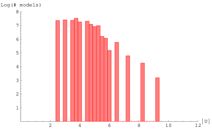
Figure 1: Number of solutions found depending on the absolute value of the complex structure variables $U_{I}$.

Note that in this procedure we have to chose a fixed set of complex structures $U_{I}$ from the very beginning. To find all solutions we have therefore to loop over all possible values for them. This is exactly the point where the bad scaling of our algorithm leads to trouble. The time to compute solutions grows exponentially with $U_{I}$. Within a total computing time of more than six months on a high performance computer cluster we have only been able to compute solutions up to an absolute value for $U_{I}$ of 12. The only point that saves our day is the experimental fact that the number of solutions decreases exponentially with the absolute value of the complex structures, as can be seen in figure 1. Being interested in a statistical statement for the full ensemble of solutions we do not have to worry about the fact that we have missed some solutions with higher complex structures, because their influence on the distribution of observables is negligible.

4 Results

Using the algorithm described in the last section we calculated a total number of $\approx 1.6\times 10^{8}$ models. Using this data we can now try to analyze the observables of these models. The total rank $r$ of the gauge group for example is given by $r=\sum_{a}N_{a}$. The resulting distribution is shown in figure 2(a). Interesting is the suppression of odd values for the total rank. This can be explained by the K-theory constraints and the observation that the generic value for $Y^{I}$ is 0 or 1. Therefore equation (11) suppresses solutions with an odd value for $r$. This suppression from the K-theory constraints is quite strong, the number of solutions reduces by a factor of six compared to the situation where these constraints are not enforced.

Another interesting quantity is the distribution of $U(M)$ gauge groups, shown in figure 2(b). We find that most models carry at least one $U(1)$ gauge group, corresponding to a single brane, and stacks with a higher number of branes become more and more unlikely. This could have been expected because small numbers occur with a much higher frequency in the partition and factorization of natural numbers.

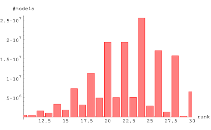
(a) Rank distribution

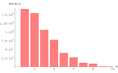
(b) $U(M)$ distribution

Figure 2: Frequency distributions of total rank and $U(M)$ gauge groups of all models.

4.1 Standard Model-like configurations

The special subset of models we are most interested in consists of those which show some properties of the Standard Model or, to be more precise, of the MSSM, since we are considering supersymmetric models only. To realize the gauge group of the Standard Model we need generically four stacks of branes (denoted by a,b,c,d) with two possible choices for the gauge groups: $U(3)_{a}\times U(2)_{b}\times U(1)_{c}\times U(1)_{d}$ or $U(3)_{a}\times Sp(2)_{b}\times U(1)_{c}\times U(1)_{d}$. To exclude exotic chiral matter from the first two factors we have to impose the constraint that ${\bf Sym}_{a}$ and ${\bf Sym}_{b}$, the number of symmetric representations, have to be zero. Models with only three stacks can also be realized, but they suffer generically from having non-standard Yukawa couplings. Since we are not treating our models in so much detail and are more interested in their generic distributions, we will include these three-stack constructions in our analysis.

Another important ingredient for Standard Model-like configurations is the existence of a massless $U(1)_{Y}$ hypercharge. This is in general a combination $U(1)_{Y}=\sum_{i\in\{a,b,c,d\}}x_{i}U(1)_{i}$ of all four $U(1)$s such that the condition $\sum_{i}x_{i}N_{i}\vec{Y}_{i}=0$ is fulfilled. More concretely there are three possible ways to construct this hypercharge $Q_{Y}^{(1)}=\frac{1}{6}Q_{a}+\frac{1}{2}Q_{c}+\frac{1}{2}Q_{d}$,  $Q_{Y}^{(2)}=-\frac{1}{3}Q_{a}-\frac{1}{2}Q_{b}$  or  $Q_{Y}^{(3)}=-\frac{1}{3}Q_{a}-\frac{1}{2}Q_{b}+Q_{d}$,  where choices 2 and 3 are only available for the first choice of gauge groups. In total we have four ways to realize the Standard Model with massless hypercharge.

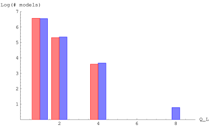
Figure 3: Number of quark and lepton generations with (red bars on the left) and without (blue bars on the right) enforcing a massless $U(1)$ .

The first question one would like to ask, after having defined what a ”Standard Model” is in our setup, concerns the frequency of such configurations in the space of all solutions. Put differently: How many Standard Models with three generations of quarks and leptons did we find?. The answer to this question is zero, even if we relax our constraints and allow for a massive hypercharge (which is rather fishy from a phenomenological point of view). The result of the analysis can be seen in figure 3. This is a rather strange result, since we know that models with three families have already been constructed in our setup (e.g. [10]). A detailed analysis of the models in the literature shows that all models which are known use (in our conventions) large values for the complex structure variables $U_{I}$ and therefore did not appear in our analysis (see section 3.1). On the other hand we know that the number of models decreases exponentially with higher values for the complex structures. Therefore we conclude that Standard Models with three generations are highly suppressed in this specific setup, more specifically the suppression factor can be estimated to be about $10^{-9}$ (cf. [4], section 5.1).

4.2 Hidden sector

Although we did not find a nice three generation Standard Model in our analysis, it might still be interesting to ask questions about the hidden sector of these models. As has been realized in [4] many of the properties of our models can be regarded to be independent of each other, which means that the statistical analysis of the hidden sector of any model with specific visible gauge group would lead to very similar results. This is indeed the case, as can be seen in figure 4. Moreover, comparing this result with the distributions of the full set of models (figure 2) shows that qualitatively the restriction to a specific visible sector does not change the distribution of gauge group observables.

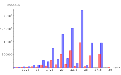
(a) Rank distribution

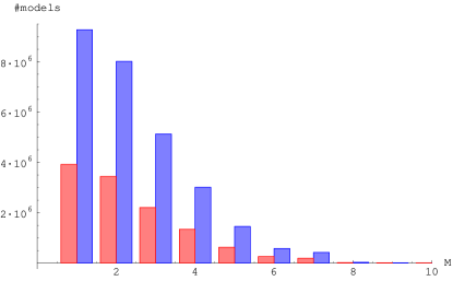
(b) $U(M)$ distribution

Figure 4: Frequency distributions of total rank and $U(M)$ gauge groups in the hidden sector of MSSM-models (red bars on the left) and MSSM models with massive $U(1)$ (blue bars on the right).

The frequency distributions of the hidden sector might be compared with a similar analysis for Gepner models carried out in [5]. To do a direct comparison with their results, we have to restrict the number of branes in the hidden sector to a maximum of three. The resulting distribution turns out to be qualitatively very similar to the Gepner model results, although our ensemble of models is much smaller and not restricted to three generation models.

4.3 Gauge couplings

The gauge sector observables considered in the last paragraphs all belong to the topological sector of the theory, in the sense that they are defined by the wrapping numbers of the branes and independent of the geometric moduli. This does not apply to the gauge couplings, which explicitly do depend on the complex structures, following the derivation in [11], which in our conventions reads

$$\frac{1}{\alpha_{a}}=\frac{M_{Planck}}{2\sqrt{2}M_{s}\kappa_{a}}\,\frac{1}{c\sqrt{\prod_{i=1}^{3}R_{1}^{(i)}R_{2}^{(i)}}}\sum_{I=0}^{3}X^{I}U_{I},$$ (14)

where $\kappa_{a}=1$ or $2$ for an $U(N)$ or $Sp(2N)$ stack respectively.

If one wants to perform an honest analysis of the coupling constants, one would have to compute their values at low energies using the renormalization group equations. We will not do this here, but instead look at the distribution of $\alpha_{s}/\alpha_{w}$ at the string scale. A value of one at the string scale does then not necessarily mean unification at lower energies, but it could be taken as a hint in this direction. The result is shown in figure 6 and it turns out that only 2.75% of all models actually do show gauge unification at the string scale.

Furthermore we would like to analyze the value of the Weinberg angle $\sin^{2}\theta=\alpha_{Y}/(\alpha_{Y}+\alpha_{w})$ depending on the ratio $\alpha_{s}/\alpha_{w}$ and check the following relation between the three couplings, which was proposed in [11] and should hold for a large class of intersecting brane models

$$\frac{1}{\alpha_{Y}}=\frac{2}{3}\frac{1}{\alpha_{s}}+\frac{1}{\alpha_{w}}\quad\leadsto\quad\sin^{2}\theta=\frac{3}{2}\,\frac{1}{\alpha_{w}/\alpha_{s}+3}.$$ (15)

The result is shown in figure 6, where we included a red line that represents the relation (15). The fact that actually 88% of all models obey this relation is a bit obscured by the plot, because each dot represents a class of models and small values for $\alpha_{s}/\alpha_{w}$ are highly preferred (cf. figure 6).

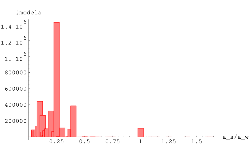
Figure 5: Frequency distribution of $\alpha_{s}/\alpha_{w}$ in Standard Model-like configurations.

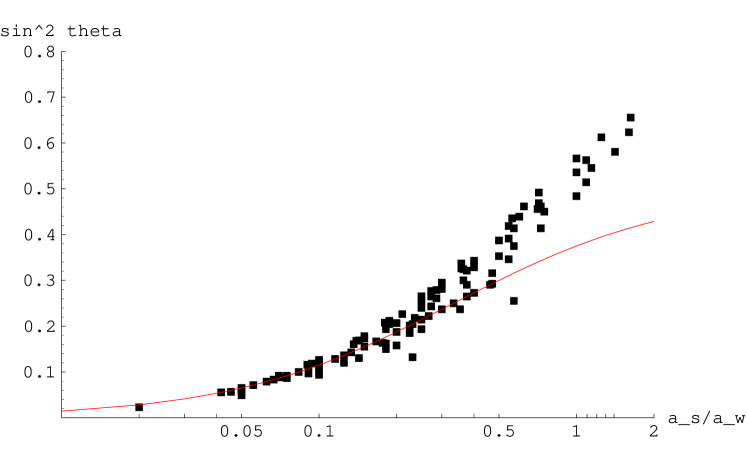
Figure 6: Values of $sin^{2}\theta$ depending on $\alpha_{s}/\alpha_{w}$. Each dot represents a class of models with these values.

Comparing these results with the Gepner model analysis of [5] we find, in contrast to the case of hidden sector gauge groups (see section 4.2), no agreement. The fraction of models obeying (15) was found to be only about 10% in the Gepner model case. This might be traced back to the observation that in contrast to the topological data of gauge groups we are dealing with geometrical aspects here, which are more influenced by the fact that we are working in a large radius regime, while the Gepner model analysis is done at small radius.

4.4 Correlations

An interesting question that we raised in the introduction concerns the correlation of observables. If different properties of our models were correlated, independently of the specific visible gauge group, this would provide us with some information about the generic behavior of this class of models. As it turns out, this is indeed the case. A nice example is the correlation between the total rank of the gauge group and the ”mean chirality” of a model. The mean chirality is a quantity defined as $\chi:=n\sum_{a\neq b}(I_{a^{\prime}b}-I_{ab})$, where $n$ is some normalization. The difference between the two intersection numbers computes the amount of chiral matter in a bifundamental representation between the stacks $a$ and $b$. $\chi$ measures therefore the amount of chirality that is present in a specific model. Looking at the distribution of models for specific values of rank and chirality we find that their values are not independent. Moreover, this behavior is generic and the shape of figure 7 does not change if we require a different visible sector gauge group.

Figure 7: Frequency distribution of models with Standard Model gauge group depending on total rank and chirality.

5 Conclusions

We presented some aspects of an explicit statistical analysis of a specific construction in the class of type II orientifold models. An interesting result is that models with three generations of Standard Model particles are highly suppressed in this setup. We found that the observables in the hidden sector are independent of the specific gauge group in the visible sector. Furthermore we found evidence for a correlation between observables. Comparing our results to the small radius analysis of Gepner models in [5] we find agreement for topological quantities, but disagreement for more geometrical properties like the gauge couplings, as could have been expected.

It would be very interesting to compare these results with statistical data of other constructions, like heterotic compactifications. Equally desirable would be the inclusion of fluxes in our statistical treatment and the analysis of grand unified gauge groups like $SU(5)$ in the visible sector.

I would like to thank the organizers of the RTN network conference Constituents, Fundamental Forces and Symmetries of the Universe in Corfu, Greece for the invitation. I am grateful to Ralph Blumenhagen, Gabriele Honecker, Dieter Lüst and Timo Weigand for collaboration on this project.

References

- [1] R. Blumenhagen, M. Cvetic, P. Langacker, and G. Shiu, “Toward realistic intersecting D-brane models,” hep-th/0502005.
- [2] M. Grana, “Flux compactifications in string theory: A comprehensive review,” hep-th/0509003.
- [3] M. R. Douglas, “The statistics of string / M theory vacua,” JHEP 05 (2003) 046, hep-th/0303194.
- [4] F. Gmeiner, R. Blumenhagen, G. Honecker, D. Lüst and T. Weigand, “One in a billion: MSSM-like D-brane statistics,” hep-th/0510170.
-
[5]
T. P. T. Dijkstra, L. R. Huiszoon, and A. N. Schellekens,
“Chiral supersymmetric Standard Model spectra from orientifolds of Gepner models,”
Phys. Lett. B609 (2005) 408–417,
hep-th/0403196;
T. P. T. Dijkstra, L. R. Huiszoon, and A. N. Schellekens, “Supersymmetric Standard Model spectra from RCFT orientifolds,” Nucl. Phys. B710 (2005) 3–57, hep-th/0411129. - [6] M. Cvetic, G. Shiu, and A. M. Uranga, “Chiral four-dimensional N = 1 supersymmetric type IIA orientifolds from intersecting D6-branes,” Nucl. Phys. B615 (2001) 3–32, hep-th/0107166.
- [7] R. Blumenhagen, F. Gmeiner, G. Honecker, D. Lüst, and T. Weigand, “The statistics of supersymmetric D-brane models,” Nucl. Phys. B713 (2005) 83–135, hep-th/0411173.
- [8] A. M. Uranga, “D-brane probes, RR tadpole cancellation and K-theory charge,” Nucl. Phys. B598 (2001) 225–246, hep-th/0011048.
- [9] M. R. Garey and D. S. Johnson, Computers and Intractability, a Guide to the Theory of NP-Completeness. Freeman San Francisco, 1979.
-
[10]
R. Blumenhagen, D. Lüst, and T. R. Taylor,
“Moduli stabilization in chiral type IIB orientifold models with fluxes,”
Nucl. Phys. B663 (2003) 319–342,
hep-th/0303016;
J. F. G. Cascales and A. M. Uranga, “Chiral 4d N = 1 string vacua with D-branes and NSNS and RR fluxes,” JHEP 05 (2003) 011, hep-th/0303024;
F. Marchesano and G. Shiu, “Building MSSM flux vacua,” JHEP 11 (2004) 041, hep-th/0409132;
M. Cvetic, T. Li, and T. Liu, “Standard-like models as type IIB flux vacua,” Phys. Rev. D71 (2005) 106008, hep-th/0501041. - [11] R. Blumenhagen, D. Lüst, and S. Stieberger, “Gauge unification in supersymmetric intersecting brane worlds,” JHEP 07 (2003) 036, hep-th/0305146.