Renormalization of the Vector Current in QED

Abstract

It is commonly asserted that the electromagnetic current is conserved and therefore is not renormalized. Within QED we show (a) that this statement is false, (b) how to obtain the renormalization of the current to all orders of perturbation theory, and (c) how to correctly define an electron number operator. The current mixes with the four-divergence of the electromagnetic field-strength tensor. The true electron number operator is the integral of the time component of the electron number density, but only when the current differs from the $\overline{\rm MS}$-renormalized current by a definite finite renormalization. This happens in such a way that Gauss’s law holds: the charge operator is the surface integral of the electric field at infinity. The theorem extends naturally to any gauge theory.

I Introduction

A classic statement about the electromagnetic current in quantum field theory is that because it is conserved it needs no renormalization — see, e.g., (sterman, , p. 341), (peskin.schroeder, , p. 430), (pokorski, , Sec. 10.1), and (hqbook, , p. 16). In fact this result is false, as we will explain in detail. Under renormalization, the current may mix with operators of equal or lower dimension whose four-divergence vanishes identically, i.e., without use of the equations of motion. As observed in (collins, , p. 162) there are no such operators in the absence of gauge fields, and so the nonrenormalization theorem holds in nongauge theories. The theorem also extends to pure QCD for the flavor currents, where the available operators all have nonzero color.

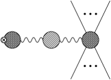
(a)	(b)	(c)

Figure 1: (a) Graphs that are one-particle-irreducible in the current channel for insertion of a current vertex in a Green function or matrix element; the standard nonrenormalization argument applies only to these. (b) These graphs, one-particle-reducible in the current channel, also contribute to matrix elements of the current and to its renormalization. The two subgraphs that are cross hatched are irreducible in the photon line, while the other subgraph gives the full propagator corrections to the photon propagator. (c) Counterterm to (b). The filled square corresponds to an operator proportional to $\partial_{\nu}F^{\nu\mu}$.

However in QED (and therefore in the full Standard Model), the current does mix with the four-divergence of the electromagnetic field-strength tensor, $\partial_{\nu}F^{\nu\mu}$. The mixing is associated with “penguin graph” contributions to matrix elements, Fig. 1(b). The conventional proof sterman of nonrenormalization ignores such graphs. Similar statements apply in more general theories .

In this article, we explain the necessary modifications, to all orders of perturbation theory, for the electron number current in QED with a single lepton flavor. (The results generalize readily to multiple lepton flavors.) There is a series of inter-related results:

• The current needs ultraviolet (UV) renormalization, by the addition of a counterterm proportional to $\partial_{\nu}F^{\nu\mu}$. The coefficient can be set in terms of the coupling and the $Z_{3}$ coefficient in the Lagrangian.

• The renormalization is by addition of an operator that does not affect the Ward identities. Nevertheless, after the application of equations of motion to the renormalized current operator in physical matrix elements, the renormalization is effectively multiplicative.

• If $\overline{\rm MS}$-renormalization is used, the current has a nonzero anomalous dimension.

• Renormalization also affects the normalization of the charge operator for electron number, unless the photon has a nonzero mass. The main part of this result was first found by Lurié (lurie, , p. 371, Eq. ((8(35))).

• There is a unique finite correction to the counterterm’s coefficient that both removes the anomalous dimension and produces a correct electron number operator that is the integral of an electron number density. In effect we have to subtract contributions associated with vacuum polarization.

• Thus the Noether current for electron number is not the correct operator to define electron number. A notable illustration is in multi-flavor QED, where, for example, the total muon number of a one-electron state is nonzero, as computed from the standard Noether current.

• The counterterm restores the Gauss’s law relation between total charge and the flux of the electric field at infinity.

• Although the effect on the total number operator, as opposed to the local current, only occurs when the photon mass is exactly zero, it depends neither on infrared (IR) divergences as such nor on UV divergences. It occurs even in a space-time dimension greater than 4, where there are no soft divergences in the scattering matrix, and with a spatial-lattice cutoff, which removes all UV problems.

• A simple standard argument involving equal-time canonical anticommutators, appears to show that the electron number of states is not renormalized, contrary to reality. We resolve this paradox, which was first found by Weeks weeks (see appendix).

The possibility that problems exist can be motivated by the standard proof that the electron-number operator is time-independent:

$$\frac{{\rm d}Q}{{\rm d}t}=\int{\rm d}^{3}\mathbf{x}\ \frac{\partial j^{0}}{\partial t}=-\int{\rm d}^{3}\mathbf{x}\ \bm{\nabla}\cdot\mathbf{j}=-\int_{\infty}{\rm d}^{2}\mathbf{\Sigma}\cdot\mathbf{j},$$ (1)

where the surface term is usually dropped. But masslessness of the gauge field allows a nonzero surface term. As we will see in detail, such a term does in fact arise, from penguin graphs, Fig. 1(b). Although the left-hand bubble in Fig. 1(b) vanishes quadratically as the external momentum $q$ at the current vertex goes to zero, there is a pole at $q^{2}=0$ in the photon propagator. In addition, the penguin graphs need nontrivial UV renormalization, with the counterterm graphs shown in Fig. 1(c)

Although our results are quite elementary, and should be well-known, the only textbook account we have found is by Lurié (lurie, , p. 371). Since current operators are auxiliary operators used to analyze a theory, the nontrivial renormalization of the current does not have direct effects on the scattering matrix and cross sections. Weeks’s paradox does symptomize some deep complications in the correct definition of states in a gauge theory.

However, many practical calculations use the operator product expansion and factorization methods. Then matrix elements of currents and related operators are used, so that incorrect theoretical expectations for anomalous dimensions will affect predictions. Beneke and Neubert Beneke.Neubert indeed found closely related effects in their analysis of $B$ decays, and remarked (without further comment) that quark number currents have nonzero anomalous dimensions in the presence of electromagnetic interactions.

II General argument

We use the standard gauge-fixed Lagrangian density

$$\mathcal{L}={} \bar{\psi}^{(0)}\left(i\gamma\cdot\partial+e_{0}\gamma\cdot A^{(0)}-m_{0}\right)\psi^{(0)}$$

$$-\frac{1}{4}\left(F_{\mu\nu}^{(0)}\right)^{2}-\frac{1}{2\xi}(\partial\cdot A)^{2}$$ (2)

$$={} Z_{2}\bar{\psi}\left(i\gamma\cdot\partial+e\mu^{\epsilon}\gamma\cdot A-m_{0}\right)\psi$$

$$-\frac{Z_{3}}{4}\left(F_{\mu\nu}\right)^{2}-\frac{1}{2\xi}(\partial\cdot A)^{2}.$$ (3)

Our conventions are that a superscript ⁽⁰⁾ (or subscript in $e_{0}$ and $m_{0}$) denotes bare quantities, dimensional regularization is in $4-2\epsilon$ dimensions, and the $\gamma$-matrices in $n$-dimensions are normalized to obey ${\rm Tr}(\gamma_{\mu}\gamma_{\nu})=4g_{\mu\nu}$. Note that the bare and renormalized couplings obey $e_{0}=e\mu^{\epsilon}Z_{3}^{-1/2}$, with $\mu$ being the usual unit of mass, and that the gauge fixing term has no counterterm. We will use $\overline{\rm MS}$-renormalization for the interactions, although this will not be essential: one formula for the current will be in an explicitly renormalization-scheme-independent form. The vacuum matrix element of a time-ordered product of operators is denoted as $\left\langle T\Bigl{\{}\,\dots\Bigr{\}}\right\rangle$. (The time-ordered product is actually the covariant $T^{*}$ product, as naturally arises with Feynman graphs or from a functional integral solution of the theory.)

The standard Noether current for electron number is $j_{\rm N}^{\mu}=\bar{\psi}^{(0)}\gamma^{\mu}\psi^{(0)}=Z_{2}\bar{\psi}\gamma^{\mu}\psi$, and it obeys a Ward identity:

$$\frac{\partial}{\partial x^{\mu}}\left\langle T\Bigl{\{}\,j_{\rm N}^{\mu}(x)\prod_{i=1}^{m}\psi(y_{i})\prod_{j=1}^{m}\bar{\psi}(z_{j})\prod_{k=1}^{l}A(w_{k})\Bigr{\}}\right\rangle={} -\sum_{i^{\prime}=1}^{m}\delta^{(4)}(x-y_{i^{\prime}})\left\langle T\Bigl{\{}\,\prod_{i=1}^{m}\psi(y_{i})\prod_{j=1}^{m}\bar{\psi}(z_{j})\prod_{k=1}^{l}A(w_{k})\Bigr{\}}\right\rangle$$

$$+\sum_{j^{\prime}=1}^{m}\delta^{(4)}(x-z_{j^{\prime}})\left\langle T\Bigl{\{}\,\prod_{i=1}^{m}\psi(y_{i})\prod_{j=1}^{m}\bar{\psi}(z_{j})\prod_{k=1}^{l}A(w_{k})\Bigr{\}}\right\rangle.$$ (4)

Because this formula is homogeneous in the fields, it applies equally whether the fields used in the Green function with the Noether current are bare or renormalized fields; but the normalization of the Noether current itself is fixed. Finiteness of the right-hand side might lead one to conclude incorrectly that Green functions (and hence matrix elements) of $j_{\rm N}^{\mu}$ are finite, so that the current is not renormalized. Certainly an extra multiplicative factor is excluded sterman ; pokorski ; collins , and a closely related argument proves that the sum of nonpenguin graphs Fig. 1(a) is finite: the factor $Z_{2}$ in $Z_{2}\bar{\psi}\gamma^{\mu}\psi$ takes care of divergences in these graphs.

But it is possible to have a counterterm proportional to an operator whose four-divergence vanishes identically (i.e., without the use of the equations of motion). If the equations of motion were needed to prove the vanishing of the four-divergence of a counterterm, extra divergent terms would appear on the right-hand side of the Ward identity.

In QED there is available a possible counterterm operator with the appropriate dimension and symmetry properties: $\partial_{\nu}F^{\nu\mu}$. The associated divergence is in the left-hand bubble of Fig. 1(b), with its vertex for the Noether current. It is evidently closely related to vacuum polarization and hence to the wave function renormalization factor $Z_{3}$ for the photon field. The counterterm operator appears in graphs of the form of Fig. 1(c). Its coefficient can be determined by the operator equation of motion for the renormalized photon field:

$$0=\frac{\delta S}{\delta A_{\mu}(x)}=e\mu^{\epsilon}j_{\rm N}^{\mu}+Z_{3}\partial_{\nu}F^{\nu\mu}+\frac{1}{\xi}\partial^{\mu}\partial\cdot A,$$ (5)

where $S=\int{\rm d}^{4-2\epsilon}x\,\mathcal{L}$ is the action for the theory. Hence, uniqueness of expansions in poles at $\epsilon=0$ shows that the $\overline{\rm MS}$-renormalized current is

$$j^{\mu}_{\overline{\rm MS}}=Z_{2}\bar{\psi}\gamma^{\mu}\psi+\frac{Z_{3}-1}{e\mu^{\epsilon}}\partial_{\nu}F^{\nu\mu},$$ (6)

in terms of which the photon equation of motion has a simple form in terms of finite operators:

$$0=e\mu^{\epsilon}j_{\overline{\rm MS}}^{\mu}+\partial_{\nu}F^{\nu\mu}+\frac{1}{\xi}\partial^{\mu}\partial\cdot A.$$ (7)

Now the use of the operator equations of motion induces extra delta function terms when applied in Green functions. However this is not the case in matrix elements. Moreover, the Gupta-Bleuler condition gives zero physical matrix elements for $\partial\cdot A$. So we can eliminate either one of the operators in Eq. (6) in favor of the other, plus a term that vanishes in physical matrix elements:

$$j^{\mu}_{\overline{\rm MS}}={} -\frac{\partial_{\nu}F^{\nu\mu}}{e\mu^{\epsilon}}-\frac{1}{\xi e\mu^{\epsilon}}\partial^{\mu}\partial\cdot A.$$ (8)

$$={} \frac{1}{Z_{3}}j_{\rm N}^{\mu}-\frac{1-Z_{3}^{-1}}{\xi e\mu^{\epsilon}}\partial^{\mu}\partial\cdot A.$$ (9)

Thus in physical matrix elements, the renormalized current obeys:

$$j^{\mu}_{\overline{\rm MS}}=-\frac{\partial_{\nu}F^{\nu\mu}}{e\mu^{\epsilon}}=\frac{1}{Z_{3}}j_{\rm N}^{\mu}\qquad\mbox{(in physical ME)}.$$ (10)

The formulae with only gauge fields exhibit the finiteness of the renormalized current, while those with the Noether current exhibit the nontrivial renormalization of the current

One further useful result is the expression of the current in terms of bare fields:

$$j^{\mu}_{\overline{\rm MS}}=\bar{\psi}^{(0)}\gamma^{\mu}\psi^{(0)}+\frac{1-Z_{3}^{-1}}{e_{0}}\partial_{\nu}F^{(0)\,\nu\mu}.$$ (11)

The multiple formulae for the current lend themselves to different interpretations. Within Feynman graph calculations, the distinction between a counterterm proportional to $\partial_{\nu}F^{\nu\mu}$ and one proportional to $j_{\rm N}^{\mu}$ is absolutely clear and unambiguous: Thus the left-hand bubble of Fig. 1(b) is renormalized using the $\partial_{\nu}F^{\nu\mu}$ operator, not $j_{\rm N}^{\mu}$. But after applying the equations of motion, the distinction is not so clear cut. Indeed, using the formula for the renormalized current in terms of the Noether current will lead us to Weeks’ paradox in Sec. A.

III One-loop verification

In a one-electron state, the one-loop matrix element of the electron number current has contributions from wave-function and vertex graphs, Fig. 2, and from a penguin graph Fig. 3. As is well-known, the UV-infinite parts of the wave-function and vertex graphs cancel. Moreover, at zero momentum transfer in an on-shell state, the complete vertex and wave function graphs cancel, so that they make no contribution, for example, to the expectation value of the electron number operator.

Figure 2: One-loop wave-function and vertex corrections.

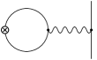
Figure 3: One-loop penguin graph contributing to the renormalization of the vector current. The cross denotes an insertion of the vector current.

However, the penguin graph also contributes. Its 1PI part is

$$\frac{eS_{\epsilon}\mu^{-\epsilon}}{2\pi^{2}}\left(-q^{2}g^{\mu\nu}+q^{\mu}q^{\nu}\right)\times$$

$$\left\{\frac{1}{6\epsilon}-\int_{0}^{1}{\rm d}x\ x(1-x)\ln\left[\frac{m^{2}-q^{2}x(1-x)}{\mu^{2}}\right]+\mathcal{O}(\epsilon)\right\},$$ (12)

where $S_{\epsilon}=(4\pi e^{-\gamma_{E}})^{\epsilon}$. The graph has a divergence which is canceled by the $\overline{\rm MS}$-counterterm in Eq. (6) with

$$Z_{3}=1-\frac{e^{2}S_{\epsilon}}{12\pi^{2}\epsilon}+\mathcal{O}(e^{4}).$$ (13)

Here we use the usual QCD definition of $\overline{\rm MS}$-renormalization that the counterterms contain a factor of $S_{\epsilon}$ for each loop.

IV Apparent Electron Number Anomaly

From our calculations, we can see that the penguin graph contribution to the matrix element of the current apparently changes the value of electron number, no matter whether we use the Noether current itself or the $\overline{\rm MS}$-renormalized current. For the total electron number we need the limit as $q^{2}\to 0$. Although the loop vanishes at $q^{2}=0$, this is canceled by the pole in the photon propagator. Thus the matrix element of $j^{\mu}_{\overline{\rm MS}}$ in a single-electron state at zero momentum transfer (and $\epsilon=0$) is

$$\langle e|j^{\mu}_{\overline{\rm MS}}|e\rangle=\left[1+\frac{e^{2}}{12\pi^{2}}\ln\left(\frac{m^{2}}{\mu^{2}}\right)+\mathcal{O}(e^{4})\right]2p^{\mu}$$ (14)

so that the electron number of an electron is apparently

$$1+\frac{e^{2}}{12\pi^{2}}\ln\left(\frac{m^{2}}{\mu^{2}}\right)+\mathcal{O}(e^{4}).$$ (15)

This is not even renormalization-group invariant. Therefore we cannot interpret the current as corresponding to electron number in the standard way, despite the fact that the current has the correct Ward identity that corresponds to the standard commutation relations between the current and the fields.

The structure of the graphs in Fig. 1 shows that the factor (15) is universal between different matrix elements of the current and charge.

An even more dramatic and paradoxical consequence occurs if we add a second flavor of fermion, which we can call a muon. The matrix element of the muon-number current has a contribution from a graph of the form of Fig. 3, with the electron loop replaced by a muon loop. Thus the muon number of the electron appears to be nonzero.

It is also useful to examine the RG properties of the $\overline{\rm MS}$-renormalized current. Its anomalous dimension can be related to the RG of the interaction by use of Eq. (11):

$$\mu\frac{{\rm d}}{{\rm d}\mu}j^{\mu}_{\overline{\rm MS}}=2\gamma_{A}\frac{\partial_{\nu}F^{(0)\,\nu\mu}}{e_{0}Z_{3}}=2\gamma_{A}\frac{\partial_{\nu}F^{\nu\mu}}{e\mu^{\epsilon}},$$ (16)

where $\gamma_{A}$ is the anomalous dimension of the photon field:

$$\gamma_{A}(e)=\frac{1}{2Z_{3}}\mu\frac{{\rm d}Z_{3}}{{\rm d}\mu}=\frac{e^{2}S_{\epsilon}}{12\pi^{2}}+\mathcal{O}(e^{4}),$$ (17)

which is related to the QED $\beta$-function by

$$\mu\frac{{\rm d}e}{{\rm d}\mu}=-\epsilon e+\beta(e)=-\epsilon e+e\gamma_{A}(e).$$ (18)

The nonzero anomalous dimension of the current, in Eq. (16), is consistent with the renormalized equations of motion, Eq. (5). We see this by use of the relations between $\beta$ and $\gamma_{A}$, together with the anomalous dimension of the gauge-fixing parameter, ${\rm d}\xi/{\rm d}\mu=-2\gamma_{A}$:

$$0={} \mu\frac{{\rm d}}{{\rm d}\mu}\left(\partial_{\nu}F^{\nu\mu}+e\mu^{\epsilon}j^{\mu}_{\overline{\rm MS}}+\frac{1}{\xi}\partial^{\mu}\partial\cdot A\right)$$

$$={} \gamma_{A}\left(\partial_{\nu}F^{\nu\mu}+e\mu^{\epsilon}j^{\mu}_{\overline{\rm MS}}+\frac{1}{\xi}\partial^{\mu}\partial\cdot A\right).$$ (19)

The right-hand side is proportional to the equation of motion, so that it vanishes. Finally, applying Eq. (10) gives a renormalization group equation for the current in terms of itself when physical matrix elements are taken:

$$\mu\frac{{\rm d}}{{\rm d}\mu}j^{\mu}_{\overline{\rm MS}}=-2\gamma_{A}\ j^{\mu}_{\overline{\rm MS}}\qquad\mbox{(in physical ME)}.$$ (20)

V Redefinition of current

Since the apparent anomaly arises from penguin-graph contributions only when the photon is exactly massless, a more satisfactory definition of the current evidently requires us to remove the penguin graph contributions. To preserve the locality of the current, we can perform an exact removal only at one value of $q$, naturally $q=0$. We will demonstrate that the correct definition (only valid if the electron mass $m$ is nonzero) is:

$$j^{\mu}={} j^{\mu}_{\overline{\rm MS}}-\frac{\Pi(0)\,\partial_{\nu}F^{\nu\mu}}{e\mu^{\epsilon}}$$

$$={} j^{\mu}_{\rm N}+\left[Z_{3}-1-\Pi(0)\right]\frac{\partial_{\nu}F^{\nu\mu}}{e\mu^{\epsilon}}$$

$$={} \bar{\psi}^{(0)}\gamma^{\mu}\psi^{(0)}+\left[1-\frac{1+\Pi(0)}{Z_{3}}\right]\frac{\partial_{\nu}F^{(0)\,\nu\mu}}{e_{0}}.$$ (21)

Here $\Pi(q^{2})$ is the vacuum polarization, defined as usual so that the renormalized photon propagator is

$$\frac{i\left(-g_{\mu\nu}+q_{\mu}q_{\nu}/q^{2}\right)}{q^{2}\,[1+\Pi(q^{2})]}-\frac{iq_{\mu}q_{\nu}\xi}{(q^{2})^{2}}.$$ (22)

The first form of $j^{\mu}$ in Eq. (V) shows that it is a finite operator that obeys the standard Ward identity, Eq. (II). In the last form, the factor $[1+\Pi(0)]/Z_{3}$ is the inverse of the photon-pole residue in the propagator of the bare photon field. Thus the last form is written solely in terms of bare quantities, so that the current is RG invariant. Moreover we have a formula where a nontrivial correction is manifestly needed even if there are no UV divergences, as when $n<4$.

The extra photon term in the definition of the current depends on the dynamics of QED, so we call it the dynamical term in the current. Its normalization is only known after the theory is solved, and depends on specifically quantum mechanical effects.

In physical matrix elements, the equation of motion for the photon field gives

$$j^{\mu}={} -\frac{[1+\Pi(0)]\ \partial_{\nu}F^{\nu\mu}}{e\mu^{\epsilon}}$$

$$={} [1+\Pi(0)]\ j^{\mu}_{\overline{\rm MS}}$$

$$={} \frac{1+\Pi(0)}{Z_{3}}\ j^{\mu}_{\rm N}$$

$$={} -\frac{\partial_{\nu}F^{\nu\mu}_{\rm phys}}{e_{\rm phys}}\qquad\mbox{(all in physical ME)}.$$ (23)

In the last line, we use what we term a physically normalized field,

$$F^{\nu\mu}_{\rm phys} = [1+\Pi(0)]^{1/2}F^{\nu\mu},$$ (24)

whose photon pole has unit residue. The corresponding coupling is

$$e_{\rm phys} = [1+\Pi(0)]^{-1/2}e\mu^{\epsilon},$$ (25)

which has the conventional value, i.e., $1.6022\dots\times 10^{-19}\,{\rm C}$, rather than the $\overline{\rm MS}$-renormalized coupling $e$ that is appropriate in certain high-energy calculations. Since, with $\overline{\rm MS}$-renormalization,

$$\Pi(0)=-\frac{e^{2}}{12\pi^{2}}\ln\frac{m^{2}}{\mu^{2}}+\mathcal{O}(e^{4}),$$ (26)

we verify that the redefinition Eq. (V) does indeed remove the one-loop anomaly in the electron number.

To see that the current $j^{\mu}$ defined in Eq. (V) is the uniquely correct current, we express an arbitrary Green function or matrix element of $j^{\mu}$ in terms of $G_{1\gamma{\rm I}}^{\mu}$, which is the 1-photon-irreducible part in the current channel. The reducible graphs are those shown in Fig. 1(b) and (c), so that the total Green function is

$$G_{\rm tot}^{\mu}=G_{1\gamma{\rm I}}^{\mu}\frac{1+\Pi(0)}{1+\Pi(q^{2})}+G_{1\gamma{\rm I}}^{\nu}\frac{q_{\nu}q^{\mu}}{q^{2}}\frac{\Pi(q^{2})-\Pi(0)}{1+\Pi(q^{2})}.$$ (27)

Multiplying by $q_{\mu}$ gives just the irreducible contribution $q_{\mu}G_{1\gamma{\rm I}}^{\mu}$, which verifies that the Ward identities are unaffected by the extra terms used to define the physical current. But when we take a physical matrix element, current conservation shows that only the first term in Eq. (27) survives, so that the matrix element differs from the irreducible contribution by a factor $[1+\Pi(0)]/[1+\Pi(q^{2})]$, which is unity when $q^{2}=0$. The standard arguments about nonrenormalization of the current actually apply only to the 1-photon-irreducible part, Fig. 1(a), which is finite and unaffected by the addition of the dynamical photon term to the current.

To see that the extra dynamical term in the current is due to bad behavior of the current operator at spatial infinity, we can use a nonzero photon mass. Then the factor between the total and irreducible parts of a matrix element of the current becomes

$$\frac{q^{2}-m_{\gamma}^{2}+q^{2}\Pi(0)}{q^{2}-m_{\gamma}^{2}+q^{2}\Pi(q^{2})}=1+\frac{q^{2}\,[\Pi(0)-\Pi(q^{2})]}{q^{2}-m_{\gamma}^{2}+q^{2}\Pi(q^{2})},$$ (28)

where the last term, proportional to $\Pi(0)-\Pi(q^{2})$, is the contribution of the penguin graphs and of the dynamical term. Because of the photon mass in the denominator, both of these contributions vanish at $q=0$.

Finally, we observe that the formula (V) for the physical current in terms of the electromagnetic field strength shows that the time-component of the current is

$$j^{0}=\frac{\bm{\nabla}\cdot\mathbf{E}}{-e_{\rm phys}}.$$ (29)

This is the divergence of the electric field operator, with its standard normalization, in units of the (negative) charge of the electron. Integrating over all space shows that the electron number with this definition equals the value given by Gauss’s law with the standard normalization. This naturally matches with the classical limit of electromagnetism, for macroscopic phenomena.

We have defined a physical charge and current, but the necessity of nontrivial renormalization depends on whether the photon is massless or not and on whether the current or charge is considered:

• In the $3+1$ dimensional theory, the Noether current always needs UV renormalization, independently of $m_{\gamma}$.

• The counterterm never affects the Ward identities.

• When the photon mass is nonzero, the counterterm integrates to zero, so that the charge does not then actually need renormalization, and the integral of the Noether charge density gives the correct charge.

• But when the photon mass is zero:

  • Integrating the counterterm over all space gives a nonzero result, so that the charge needs UV renormalization.

  • A particular finite part in the counterterm is needed to obtain the correct charge.

  • Even when the theory is regulated in the UV, the finite renormalization of the current and charge are still needed, if the the charge is to be correct.

• However, even with a nonzero photon mass, the definition of the physical current (V) is valid and gives the correct charge. (The counterterm integrates to zero.) This definition has the practical advantages that there are no problems in taking the limits of zero photon mass, integration over all space, and removing a UV regulator, and that changing the order of limits is safe.

Evidently the need for a nontrivial renormalization of the total electron number (as opposed to the current) only arises when the photon is massless. However, it is to be emphasized that this is not due to actual infra-red divergences as normally understood. This can be seen by considering the theory in 5 space-time dimensions (i.e., 4 space dimensions), with a spatial lattice. The higher space-time dimension is sufficient to remove all the usual soft divergences in the scattering matrix. The use of an integer dimension removes all possible artifacts associated with dimensional regularization, and the use of a spatial lattice gives us a conventional quantum mechanical theory (in real time) without UV divergences. All the considerations leading to a physical current that is not equal to the Noether current still apply.

It is sometimes claimed that the actual definition of QED requires us first to regulate the theory in the IR, say with a nonzero photon mass, and then to take the limit of zero photon mass. If this were so, we could avoid the need to redefine the charge, since in the regulated theory the Noether charge would give the correct answer. However, as a field theory, QED exists if the photon mass is kept at zero at all stages; this is evidenced by the fact that the Green functions of the theory exist directly at $m_{\gamma}=0$. The use of an IR regulator (and inclusive cross sections that allow undetected soft photon emission) is only necessary if one uses the conventional LSZ formalism to compute cross sections. In any case, when the space-time dimension is above 4 there are no soft photon divergences in cross sections, but nevertheless a redefinition of the charge is still needed, as we have just seen.

Our arguments generalize to more complicated theories. For example, the approach applies to QED with more than one flavor of lepton, with suitable changes in the numbers of flavors in the vacuum polarization graphs. The approach applies not only to the electromagnetic current itself, but also to the individual conserved flavor-number currents.

We propose an interpretation of the nontrivial renormalization of the current as a universal effect of attempts to measure the current. The quantum mechanical current creates polarization of the vacuum. Although this effect is proportional to $1/r^{2}$ at a distance $r$ from a source, it has to be integrated over a sphere of surface area proportional to $r^{2}$, so that the effect is nonvanishing as $r\to\infty$.

Appendix A Weeks’ paradox

A.1 Formulation

Conventional expectations for the interpretation of a charge operator, and, in particular, for its value in a state of definite electron number arise quite generally from the commutation relations between the Noether current and bare elementary fields. These commutation relations are entirely unaffected by UV renormalization and are fundamental to the definition of a quantum field theory. Inspired by the paper of Weeks weeks , we now present a paradox.

The paradox and its resolution turn on the issue of the correct way to implement concretely the concept of the electron number of a state. There are several possible ways of implementing the concept. In scattering theory, we can use in- or out-states as basis states; the labeling of these states in the usual way gives unambiguous values for electron number. But we could also define electron number in terms of eigenvalues of a suitable operator for conserved charge. Yet another possible definition would use the expectation value of the charge in a state. In the absence gauge fields, the different definitions can be proved to agree. But, as we will see, in QED an attempt to make such a proof runs into problems. The problems are related to, but distinct from, the issues treated in the body of this paper.

The paradox is obtained as follows:

1. Let $|0\rangle$ be the (true) vacuum state and let $|1\rangle$ be any state of electron number unity. While we may use an on-shell one-electron state of definite momentum for $|1\rangle$, it is safer to use a normalizable wave-packet state. Here we chose the states to be normal in- or out-states, with electron number being defined with respect to the obvious labeling of the states in terms of particle content.

2. We assume, as is natural, that $\langle 1|\bar{\psi}|0\rangle\neq 0$, and that $|0\rangle$ and $|1\rangle$ are eigenstates of the Noether charge $Q_{\rm N}$. Of course, we have shown in the body of this paper that there is an unexpectedly nontrivial renormalization of the charge, which leads to the expectation that the eigenvalue disagrees with naive expectations. But this finding by itself does not impinge on the presumption that we have an eigenstate.

3. We (and Lurié lurie ) have calculated that the expectation value value of $Q_{\rm N}$ in the state $|1\rangle$ is $\hat{Z}_{3}$ . Here $\hat{Z}_{3}$ is the renormalization factor for the photon field in an on-shell field. It equals $Z_{3}/[1+\Pi(0)]$ in our earlier notation. An explicit one-loop calculation shows that $\hat{Z}_{3}\not=1$. Of course, on an eigenstate the expectation value of an operator equals the eigenvalue.

4. From the canonical equal-time anticommutation relations for the fermion field we find

   $$\langle 1|\bar{\psi}(t,\mathbf{x})|0\rangle={} \langle 1|\left[Q_{\rm N},\bar{\psi}(t,\mathbf{x})\right]|0\rangle$$

   $$={} \langle 1|Q_{\rm N}\bar{\psi}|0\rangle-\langle 1|\bar{\psi}\,Q_{\rm N}|0\rangle$$

   $$={} \left(\hat{Z}_{3}-0\right)\langle 1|\bar{\psi}(t,\mathbf{x})|0\rangle$$ (30)

Since $\hat{Z}_{3}\neq 1$, there is a contradiction, i.e., there is at least one mistake in the calculation or the assumptions.

Weeks’ weeks derivation of the paradox was in Coulomb gauge, but the main ideas are the same. The basic conflict is between the canonical commutation relation $\left[Q_{\rm N},\bar{\psi}\right]=1\cdot\bar{\psi}$, and the value $\hat{Z}_{3}\not=1$ for $Q_{\rm N}$ in the state $|1\rangle$.

A.2 Resolution

The resolution of the paradox is that physical states are not exactly eigenstates of the Noether charge operator $Q_{\rm N}$, contrary to the (unproved) assumption made at step 2 of the derivation of the paradox. For example, as we will see, when the charge density operator $j_{\rm N}^{0}$ is applied to the vacuum and then integrated over position, there is a certain contribution that vanishes in the limit of infinite volume (or equivalently when the momentum transfer $\mathbf{q}$ goes to zero). However, matrix elements of a field operator with this part of the state have a divergence in the same limit. Moreover this anomalous contribution is associated with unphysical parts of the theory: the unphysical states in Feynman gauge, or the instantaneous Coulomb potential in Coulomb gauge. Thus it is not easily visible when one restricts attention to physical matrix elements; in particular, the anomalous contribution does not affect the calculation of the expectation value of the charge in physical state. In addition, in Coulomb gauge the equal-time commutators and anticommutators are modified by interactions.

We will illustrate these issues by calculations of the commutators in two ways. One is the Bjorken-Johnson-Low (BJL) method BJL , which is applied to time-ordered products of the current and fields, while the second method is a direct calculation with the intermediate states used in the commutator — see Eq. (A.2.1) below.

A.2.1 Resolution in Feynman gauge

Consider first the commutator in covariant gauge between the Noether current and the electron field.

$$\langle 1|[j_{\rm N}^{0}(t,\mathbf{y}),\bar{\psi}(t,\mathbf{x})]|0\rangle={} \sum_{X}\langle 1|j_{\rm N}^{0}|X\rangle\langle X|\bar{\psi}|0\rangle$$

$$-\sum_{Y}\langle 1|\bar{\psi}|Y\rangle\langle Y|j_{\rm N}^{0}|0\rangle.$$ (31)

The sums over intermediate states are over all states, not just over representatives of the physical subspace.

The BJL method gives this matrix element of the commutator from the Fourier transform of the corresponding matrix element of the time-ordered product, by taking the limit as $q^{0}\to\infty$ of $iq^{0}$ times the matrix element. Here $q^{\mu}$ is the external momentum flowing into the vertex for $j_{\rm N}^{0}$. Thus

$$\langle 1|[j_{\rm N}^{0}(t,\mathbf{y}),\bar{\psi}(t,\mathbf{x})]|0\rangle={}$$

$$\lim_{q^{0}\to\infty}iq^{0}\int{\rm d}t\,e^{iq^{0}t}\langle 1|T\,j_{\rm N}^{0}(t,\mathbf{y}),\bar{\psi}(t,\mathbf{x})|0\rangle.$$ (32)

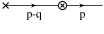
Figure 4: Matrix element on the right of Eq. (A.2.1) used in lowest-order BJL computation of the commutator. The circled cross is the vertex for the operator $j_{\rm N}^{0}$ and the simple cross is the vertex for $\bar{\psi}$. The external line of momentum $p$ is for the state $|1\rangle$.

It is readily verified that the lowest-order calculation from the graph of Fig. 4 gives the expected commutator:

$$\lim_{q^{0}\to\infty}iq^{0}\bar{u}\gamma^{0}\frac{i(p\hbox to0.0pt{\hss/}-q\hbox to0.0pt{\hss/}+m)}{(p-q)^{2}-m^{2}}=\bar{u},$$ (33)

where $u$ is the Dirac wave function for the on-shell one-electron state $|1\rangle$, of momentum $p$.

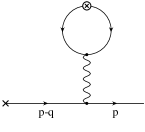
Figure 5: Graph for the one-loop vacuum-polarization contribution to the BJL computation.

The one-loop penguin graph contribution to Eq. (A.2.1) is from the graph of Fig. 5. Any correction factor to the LO result is from the large $q^{0}$ behavior of the vacuum polarization graph times the photon propagator:

$$\frac{-ig^{\mu}_{\nu}}{q^{2}}i(-g^{\nu 0}q^{2}+q^{\nu}q^{0})\Pi(q^{2})=\left(-g^{\mu 0}+\frac{q^{\mu}q^{0}}{q^{2}}\right)\Pi(q^{2}).$$ (34)

The $\mu=0$ case is

$$\frac{\mathbf{q}^{2}}{q^{2}}\Pi(q^{2}),$$ (35)

which is suppressed at large $q^{0}$ by two powers of $q^{0}$. The spatial part is

$$\frac{\mathbf{q}q^{0}}{q^{2}}\Pi(q^{2}),$$ (36)

again suppressed, but by one power of $q^{0}$.

So the canonical commutator is unchanged. But notice how the $q^{\mu}q^{0}$ part of the vacuum polarization is essential to the suppression. This contrasts with the fact that this term does not contribute to physical matrix elements of the current. We may therefore anticipate that contributions from unphysical intermediate states in Eq. (A.2.1) are essential to get the correct result.

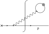
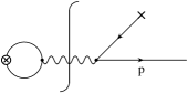
Figure 6: Graphs for the one-loop vacuum-polarization contribution to the BJL computation, with cuts on the photon line.

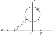
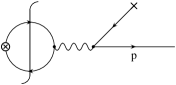
Figure 7: Graphs for the one-loop vacuum-polarization contribution to the BJL computation, with cuts on an electron-positron pair.

This can be seen explicitly from the graphs of Fig. 6, where the cuts correspond to the cases that $|X\rangle$ is an out-state of one electron and one photon, and that $|Y\rangle$ is a state of one photon. The vacuum polarization factor is

$$i(-g^{\mu 0}q^{2}+q^{\mu}q^{0})\Pi(q^{2})=iq^{\mu}|\mathbf{q}|\Pi(0),$$ (37)

given that the photon is on-shell, $q^{2}=0$. This means that in the first graph, the sole contribution is from a photon with a scalar polarization, i.e., a polarization vector proportional to its lightlike momentum. This is a state of zero norm: the current applied to the vacuum has not created a genuine photon. Moreover, in the relevant part of (A.2.1), the vacuum polarization factor (37) vanishes quadratically when $\mathbf{q}\to 0$, which is completely compatible with the natural expectation that the vacuum has zero charge, so that it is annihilated by the operator $Q_{\rm N}$.

In the commutator, this factor contributes to the matrix element $\langle Y|j_{\rm N}^{0}|0\rangle$. However it is multiplied by $\langle 1|\bar{\psi}|Y\rangle$, and then we get a nonzero result from the following dependence on $\mathbf{q}$:

• The already-derived factor of $\mathbf{q}^{2}$.

• $1/|\mathbf{q}|$ in the photon relativistic phase space.

• The IR singularity $\propto 1/|\mathbf{q}|$ in the fermion propagator in $\langle 1|\bar{\psi}|Y\rangle$.

The nonzero result at $\mathbf{q}=0$ is independent of the space-time dimension. Thus it does not depend on the existence of IR divergences that violate the standard principles for asymptotic scattering states, but only on the masslessness of the photon.

To summarize: Although the charge operator applied to the vacuum, for example, does give zero, this is compensated by an infinity in the matrix element with the field operator. Moreover the offending intermediate state is of zero norm, before taking the $\mathbf{q}\to 0$ limit, so the state is equivalent to the zero state. Similar remarks apply to the one-electron-one-photon intermediate state from the other diagram in Fig. 6.

A related issue is about the value of the commutator of the physical charge. In physical matrix elements, the two charges differ by a factor $\hat{Z}_{3}$, and it is tempting to say that the commutators also differ by this factor. But consider the expression of the physical current in terms of the Noether current and $\partial\cdot A$. This is obtained by application of the equations of motion Eq. (7) to the physical current Eq. (V), but without the physical state condition that we used in Eq. (V):

$$j^{\mu}={} \frac{1}{\hat{Z}_{3}}\ j^{\mu}_{\rm N}+\frac{\hat{Z}_{3}^{-1}-1}{\xi e\mu^{\epsilon}}\partial^{\mu}\partial\cdot A.$$ (38)

The physical electron number operator is defined as an integral over $j^{0}$, so that

$$Q_{\rm phys}={} \frac{1}{\hat{Z}_{3}}\ Q_{\rm N}+\frac{\hat{Z}_{3}^{-1}-1}{\xi e\mu^{\epsilon}}\int{\rm d}^{3}\mathbf{x}\ \partial^{0}\left(\partial\cdot A\right).$$ (39)

In physical matrix elements we can ignore the second term, to get the usual ratio of $\hat{Z}_{3}$ between the physical and Noether charges. But in commutators with elementary fields, we must include the second term. Since this second term involves a double time-derivative of the gauge field, the equations of motion must be applied to write it in terms of elementary fields and their canonical momenta, if we are to use canonical commutation and anticommutation relations. This gives extra terms, so the commutators of $Q_{\rm phys}$ and $Q_{\rm N}$ with elementary fields are not simply related by $\hat{Z}_{3}$.

The appropriate formula to use is, in fact, either of the two last lines of Eq. (V). For the $\mu=0$ component we have

$$Q_{\rm phys} = Q_{\rm N}+\left[1-\hat{Z}_{3}^{-1}\right]\int{\rm d}^{3}\mathbf{x}\frac{\partial_{\nu}F^{(0)\,\nu 0}}{e_{0}}$$

$$= Q_{\rm N}-\frac{1-\hat{Z}_{3}^{-1}}{e_{0}}\int{\rm d}^{3}\mathbf{x}\left[\mathbf{\nabla}^{2}A^{0}+\frac{\partial}{\partial t}\mathbf{\nabla}\cdot\mathbf{A}^{(0)}\right],$$

i.e., the Noether charge density, with unit normalization, plus a term that involves at most a first-order time derivative, so that it commutes at equal time with the fermion fields, to give $\left[Q_{\rm phys},\bar{\psi}\right]=\left[Q_{\rm N},\bar{\psi}\right]=\bar{\psi}$. Thus, despite the relative factor $\hat{Z}_{3}$ between the physical and Noether charges as projected onto physical states, the commutators with the fermion do not have this factor.

A.2.2 Resolution in Coulomb gauge

In the Coulomb gauge version of the BJL calculation from the graph of Fig. 5, the vacuum polarization graph times the photon propagator is now

$$\frac{i(-g^{\mu}_{\nu}+q^{\mu}v_{\nu}q^{0}/\mathbf{q}^{2})}{q^{2}}i(-g^{\nu 0}q^{2}+q^{\nu}q^{0})\Pi(q^{2}),$$ (41)

where $v^{\mu}=(1,\mathbf{0})$ is the unit vector defining the rest frame for the Coulomb gauge, and we have dropped those terms in the propagator that are exactly zero because the vacuum polarization is transverse. It is easily checked that this formula equals $-g^{\mu 0}\Pi(q^{2})$. As $q^{0}\to\infty$, this is missing the power suppression that we have in covariant gauge. If the theory is regulated in the UV, e.g., by using $\epsilon>0$, then the vacuum polarization does go to zero, so that the loop correction to the standard commutator vanishes. But after the regulator is removed, the vacuum polarization grows logarithmically.

Evidently there is an anomaly in the commutator of the Noether charge density with the field $\bar{\psi}$. Because constrained quantization is used, it is not automatically true that standard canonical commutation and anticommutation relations can be maintained. But this result depends on the space-time dimension.

Interesting dimension-independent pathologies also arise in the calculation of the commutator with intermediate states, but from electron-positron terms instead of photon terms. In the photon term, we have the same vacuum polarization factor Eq. (37) as before, but now $q^{\mu}$ times the numerator on the on-shell photon line gives exactly zero.

Instead there are extra contributions from intermediate states with electron-positron pairs, Fig. 7. The cut vacuum polarization graph has the transverse form

$$(-g^{\nu 0}q^{2}+q^{\nu}q^{0})\Pi_{c}(q^{2})=\left(\mathbf{q}^{2},\mathbf{q}\,q^{0}\right),$$ (42)

where $q^{2}$ is no longer zero, but is bounded below by $4m^{2}$. The spatial part of this vector gives zero when multiplied into the photon propagator. However, the time component multiplies a factor $i/\mathbf{q}^{2}$ for the instantaneous Coulomb potential, so that we get a nonzero limit at $\mathbf{q}=0$. Of course, the energy $q^{0}$ is nonzero, but this is allowed, since the charge operator is computed from the charge density at a fixed time, so that in momentum space there is an integral over all $q^{0}$.

The result of a nonzero limit at $\mathbf{q}=0$ is dimension independent, and again indicates that states of definite particle number are not actual eigenstates of the Noether charge. But the source of the anomaly has changed. In Feynman gauge the anomalous contribution was associated with unphysical states. But in Coulomb gauge, it is associated with the unphysically instantaneous potential in the photon propagator.

References

- (1) G. Sterman, An Introduction to quantum field theory, Cambridge University Press (1993).
- (2) M.E. Peskin and D.V. Schroeder, An Introduction to quantum field theory, Addison-Wesley (1995).
- (3) S. Pokorski, Gauge Field Theories, Cambridge University Press (2000).
- (4) A.V. Manohar and M.B. Wise, Heavy Quark Physics, Cambridge University Press (2000).
- (5) J.C. Collins, Renormalization, Cambridge University Press (1984).
- (6) D. Lurié, Particles and Fields, Wiley (1968).
- (7) B.G. Weeks, “The Apparent Double Valuedness Of The Electric Charge In QED,” SLAC-PUB-2659
- (8) M. Beneke and M. Neubert, Nucl. Phys. B 675, 333 (2003) [arXiv:hep-ph/0308039].
- (9) J.D. Bjorken, Phys. Rev. 148, 1467 (1966). K. Johnson and F.E. Low, Prog. Theor. Phys. Suppl. 37, 74 (1966).