A Planck-scale axion and SU(2) Yang-Mills dynamics: Present acceleration and the fate of the photon

Francesco Giacosa and Ralf Hofmann

Institut für Theoretische Physik
Universität Frankfurt
Johann Wolfgang Goethe - Universität
Max von Laue–Str. 1
60438 Frankfurt, Germany

From the time of CMB decoupling onwards we investigate cosmological evolution subject to a strongly interacting SU(2) gauge theory of Yang-Mills scale $\Lambda\sim 10^{-4}$ eV (masquerading as the $U(1)_{Y}$ factor of the SM at present). The viability of this postulate is discussed in view of cosmological and (astro)particle physics bounds. The gauge theory is coupled to a spatially homogeneous and ultra-light (Planck-scale) axion field. As first pointed out by Frieman et al., such an axion is a viable candidate for quintessence, i.e. dynamical dark energy, being associated with today’s cosmological acceleration. A prediction of an upper limit $\Delta t_{m_{\gamma}=0}$ for the duration of the epoch stretching from the present to the point where the photon starts to be Meissner massive is obtained: $\Delta t_{m_{\gamma}=0}\sim 2.2$ billion years.

1 Introduction

The possibility to interpret dark energy in terms of an ultra-light pseudo-Nambu-Goldstone boson field is at the center of an exciting debate stretching over the last decade, see e.g. [1, 2, 3, 4, 5, 6]. The idea is that an axion field $\phi$, which is generated by Planckian physics, develops a small mass due to topological defects of a Yang-Mills theory. If the associated Yang-Mills scale is far below the Planck mass $M_{P}$ then $\phi$’s slow-roll dynamics at late time can mimic a small cosmological constant being in agreement with the present observations. Having the coherent field $\phi$ decay by increasingly efficient self-interactions at late time, the associated very light pseudoscalar bosons interact with ordinary matter only very weakly and thus escape their detection in collider experiments. Because of a dynamically broken, global U(1)_A symmetry associated with the very existence of $\phi$ the corresponding potential $V(\phi)$ is radiatively protected. Notice that $V(\phi)$ is generated by an explicit, anomaly-mediated breaking of U(1)_A.

Up to small corrections, arising from multi-instantons effects, $V(\phi)$ has the following form [7]

$$V(\phi)=\mu^{4}\left[1-\cos\left(\frac{\phi}{F}\right)\right]\,.$$ (1)

Two mass scales enter in eq. (1): the dynamical symmetry breaking scale $F$ (axion decay constant) and a scale $\mu$ associated with the explicit symmetry breaking. The scale $\mu$ roughly determines at what momentum scale the gauge theory providing the topological defects becomes strongly interacting. Recall that the potential (1) is an effective one, arising from a quantum anomaly of the U(1)_A symmetry which is defined on integrated-out fermion fields. The anomaly becomes operative through topological defects of a Yang-Mills theory and is expressed by an additional, CP violating contribution

$$\mathcal{L}_{\phi-\mbox{\tiny}{SU(2)}}=\frac{\phi}{32\pi^{2}F}F_{\mu\nu}^{a}\widetilde{F}^{a,\mu\nu}\,.$$ (2)

Upon integrating over topological sectors, one concludes that the parameter $\mu$ in (1) is comparable to the Yang-Mills scale $\Lambda$ [7, 8].

The mass $m_{\phi}$ of the field $\phi$, as derived from (1) for the range $\left|\phi\right|\lesssim\frac{\pi}{2}F$, reads $m_{\phi}\simeq\mu^{2}/F$. Assuming $\phi\sim F\sim 10^{18}\,$GeV, the needed value for $\mu$ to generate the present density of dark energy in the universe (inferred from fits to SNe Ia luminosity distance–redshift data for $z<1.7$ [9, 10, 11]) is $\mu\sim 10^{-3}$ eV [1]. By the closeness of $\mu$’s value to the MSW neutrino mass a possible connection with neutrino physics was suggested in [1] (see also [6]).

In the present work we wish to propose a different axion-based scenario relating the (presently stabilized) temperature of the CMB, $T_{{\tiny\mbox{CMB}}}=2.35\times 10^{-4}$ eV, with the present scale of dark energy $\sim 10^{-3}\,$eV. Namely, we postulate that the gauge factor $U(1)_{Y}$ of the standard model of particle physics (SM) is only an effective manifestation of a larger gauge group. According to [12] one is lead to consider SU(2)$\supset U(1)_{Y}$ (henceforth referred to as SU(2)${}_{{\tiny\mbox{CMB}}}$) as a viable candidate for such an enlargement of the SM’s gauge symmetry. In spite of the fact that such a postulate is rather unconventional we nevertheless feel that a fruitful approach to the dark-energy problem needs novel Ansätze. In a slightly different context a QCD-like force of scale $\sim 10^{-3}\,$eV was also discussed in [4].

We intend to explore some consequences of the postulate SU(2)${}_{{\tiny\mbox{CMB}}}\overset{{\tiny\mbox{today}}}{=}$U(1)_Y in connection with axion physics. The observation of a massless and unscreened photon strongly constrains the region in the phase diagram of the SU(2) Yang-Mills theory corresponding to the present state of the Universe [12, 13]. As a consequence, the Yang-Mills scale $\Lambda_{{\tiny\mbox{CMB}}}$ is determined to be comparable to $T_{{\tiny\mbox{CMB}}}$: $\Lambda_{{\tiny\mbox{CMB}}}\sim 10^{-4}$ eV.

The fact that $T_{{\tiny\mbox{CMB}}}$ is comparable to the Yang-Mills scale of a theory with gauge group SU(2)${}_{{\tiny\mbox{CMB}}}$ (containing the U(1)_Y factor of the SM as a subgroup) which in connection with a Planck-scale axion field explains the present density of dark energy, does by itself not constitute a proof for the existence of SU(2)${}_{{\tiny\mbox{CMB}}}$ in Nature. For this setup to be convincing it ought to make independent and experimentally verified pre- and postdictions such as a dynamical account of the large-angle features of CMB maps induced by the nonabelian fluctuations of SU(2)${}_{{\tiny\mbox{CMB}}}$. In this sense the present paper is the very first stage in a long-term program exploring the implications of SU(2)${}_{{\tiny\mbox{CMB}}}\overset{{\tiny\mbox{today}}}{=}$U(1)_Y, see also [14]. The authors are well aware of the fact that this program may lead to the falsification of the postulate SU(2)${}_{{\tiny\mbox{CMB}}}\overset{{\tiny\mbox{today}}}{=}$U(1)_Y. Mounting evidence for its correctness is, however, provided by two-loop calculations of thermodynamical quantities in the deconfining phase of SU(2) Yang-Mills theory, see [13, 15], making a further pursuit of this program worthwhile.

For the reader’s convenience, let us put the results of ref. [12] into perspective with other approaches to Yang-Mills thermodynamics. First of all, it is important to note that ref. [12] considers the case of pure thermodynamics only, that is, the absence of external (static or dynamic) sources which would upset the spatial homogeneity of the system. As a consequence, the approach in [12] has nothing to say about the spatial string tension in the deconfining phase. The spatial string tension, introducing a distance scale $R$ into the system, can, however, be easily extracted in lattice simulations of the spatial Wilson loop [16, 17]. It is conceivable that static sources can be treated adiabatically based on the approach of [12] by assuming a position dependence of temperature, but this is the subject of future research. In the absence of sources, a situation that is of relevance for physics on cosmological length scales, refs. [12, 18] give a detailed and reliable account of SU(2) and SU(3) Yang-Mills thermodynamics. Lattice simulations for SU(3), using the differential method [19, 20], which is adopted to finite lattice sizes, yield quantitative agreement with the result for the entropy density (an infrared safe quantity) obtained in ref. [12]. The results for the pressure and the energy density (infrared sensitive) agree qualitatively with those obtained in [19, 20]. That is, in contrast to the integral method, which assumes the infinite-volume limit on a finite-size lattice, the pressure is negative shortly above the critical temperature in the deconfining phase, and there is a power-like fast approach to the Stefan-Boltzmann limit for $T\rightarrow\infty$. Both phenomena are observed in the approach of [12], but numerically the results differ in the vicinity of the phase boundary. By virtue of the trace anomaly the gluon condensate, up to a factor weakly depending on temperature ($\beta$-function over fundamental coupling $g$), coincides with the trace of the energy-momentum tensor $\rho-3P$. Neglecting the masses and interactions of the excitations, which is an excellent approximation at high temperatures as far as the excitation’s equation of state is concerned, we have $\rho-3P\propto T$. In [21] the temperature dependence of the SU(2) gluon condensate was investigated on the lattice, and, indeed a linear rise of the gluon condensate with temperature was observed. Notice the conceptual and technical differences of [12] to the hard-thermal-loop (HTL) approach [22]. The latter derives a nonlocal theory for interacting soft and ultrasoft modes. While the HTL approach, in a highly impressive way technically, integrates perturbative ultraviolet fluctuations into effective vertices it can not shed light on the stabilization of the infrared physics associated with nonperturbative fluctuations residing in the magnetic sector of the theory. The derivation of the phase $\phi/|\phi|$ in [12, 23], however, invokes these nonperturbative, magnetic correlations. An impressive machinery has been developed within the renormalization-group flow approach to Yang-Mills thermodynamics both in the imaginary [24] and the real-time approach [25] the latter making important observations concerning the (nonperturbative) temperature dependence of the thermal gluon mass. Interesting results for the nonperturbative temperature dependence of the fundamental gauge coupling in Quantum Chromodynamics were obtained in [26]. However, to the best of the authors knowledge, no decisive nonperturbative calculation (fully considering the magnetic sector) of the thermodynamical pressure or related quantities has yet been performed within this approach.

The paper is organized as follows: First, we briefly recall some basic nonperturbative results obtained in [12] for SU(2) Yang-Mills thermodynamics. Then we discuss the viability of our scenario when confronting it with particle-physics experiments and cosmological observations. Subsequently, we consider for a spatially flat Universe the evolution of the cosmological scale factor $a=a(t)$ and of the axion-field $\phi=\phi(t)$ from the time of decoupling $t_{dec}$ (corresponding to $z_{dec}=1089$) up to the present. We then investigate the future evolution of the Universe up to the point when the transition between the deconfining and the preconfining phase of SU(2)${}_{{\tiny\mbox{CMB}}}$ will take place and the photon will acquire a Meissner mass. Finally, we present our conclusions and an outlook on future research.

2 SU(2) Yang-Mills thermodynamics

In [12] a nonperturbative approach for SU(2)/SU(3) Yang-Mills thermodynamics is developed. For the sake of brevity we recall only some of the results relevant for the present study. Analytical expressions are reported in the Appendix.

Deconfining (electric) phase:

At high $T$ it is shown in [12, 23] that an inert adjoint Higgs field $\varphi$ emerges upon spatial coarse-graining over topological defects. The modulus of the Higgs field is (nonperturbatively) temperature dependent with $\left|\varphi_{E}\right|=\sqrt{\Lambda_{E}^{3}/2\pi T}$ (here $\Lambda_{E}$ denotes the Yang-Mills scale as defined in the deconfining phase [12]); furthermore, the field $\varphi_{E}$ induces a dynamical gauge symmetry breaking SU(2)$\rightarrow$ U(1): two of the three gauge bosons become massive (denoted by $V^{\pm}$), while the third one remains massless (denoted by $\gamma$). Massive excitations $V^{\pm}$ are very weakly interacting thermal quasi-particles, their mass depends on temperature as

$$m_{V^{\pm}}=2e(T)\left|\varphi_{E}\right|$$ (3)

where $e(T)$ is an effective temperature-dependent gauge coupling as plotted in Fig. 1.

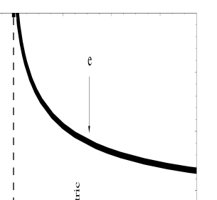
Figure 1: Temperature evolution of the effective (electric and magnetic) couplings.

The gauge coupling $e(T)$ diverges logarithmically at $T_{c,E}$ and has a plateau value of $e\simeq 8.89$ for $T\gg T_{c,E}$. For $T\searrow T_{c,E}$ the $V^{\pm}$ bosons acquire an infinite mass, $m_{V^{+}}=m_{V^{-}}\propto-\log(T_{E}-T_{c,E})$. Thus they do no longer (weakly) screen the propagation of the massless excitation $\gamma$.

Plots for the energy-density and for the pressure as functions of the dimensionless temperature $\lambda_{E}=\frac{2\pi T}{\Lambda_{E}}$ are shown in Fig. 2.

Figure 2: Ratios of Pressure (left panel) and energy density (right panel) to $T^{4}$ of an SU(2)Yang-Mills theory within the deconfining (electric) and preconfining (mangetic) phases. The vertical lines denote phase boundaries.

In Fig. 2 a jump in the energy density at the critical value $\lambda_{c,E}=13.87$ is seen. This signals a transition between the deconfining (also called electric, $T\geq T_{c,E}$) and the preconfining (also called magnetic, $T_{c,M}\leq T<T_{c,E}$) phases. Notice that for high $T$ the Stefan-Boltzmann limit is approached in a power-like fashion.

Preconfining (magnetic) phase:

In the preconfining phase the dual gauge symmetry $U(1)$ is dynamically broken by a magnetic monopole condensate, which, after spatial coarse-graining, is described by an inert complex scalar field $\varphi_{M}$ with $\left|\varphi_{M}\right|=\sqrt{\Lambda_{M}^{3}/2\pi T}.$ The dual gauge excitation $\gamma$ now acquires a Meissner mass

$$m_{\gamma}=g(T)\left|\varphi_{M}\right|,$$ (4)

where $g(T)$ is the effective coupling in the magnetic phase as shown in Fig. 1. The latter vanishes for $T\nearrow T_{c,E}$ and it diverges logarithmically for For $T\searrow T_{c,M},$ where $T_{c,M}\sim 0.83\,T_{c,E}$ in the SU(2) case.

For $T\nearrow T_{c,E}$ a jump in the number of polarizations ($3\rightarrow 2$) takes place thus explaining the discontinuity $\rho_{c,M}\rightarrow\rho_{c,E}$ in the energy density, see Fig. 2. Due to the dominance of the ground state the pressure is negative for $T\sim T_{c,E}$ (for a microscopic explanation of this macroscopically stabilized situation see [12]).

For $T\searrow T_{c,M}$ the excitation $\gamma$ becomes infinitely massive, thus signalling a second phase transition which is of the Hagedorn type.

Confining (center) phase:

For temperatures below $T_{c,M}$ the system is in its confining phase: fundamental test-charges and gauge modes are confined and decoupled, respectively. The excitations are (single and selfintersecting) fermionic center-vortex loops [12].

When confronting these results with the postulate SU(2)${}_{{\tiny\mbox{CMB}}}\overset{{\tiny\mbox{today}}}{=}$U(1)_Y the reader may be puzzled by the existence of two massive excitations in addition to the photon for $T>T_{{\tiny\mbox{CMB}}}$; however, as shown in [12] and explained in more detail in Sec. 3, the interaction between $\gamma$ and $V^{\pm}$ is tiny because the off-shellness of admissible quantum fluctuations is strongly constrained by the applied spatial coarse-graining. At $T=T_{c,E}=T_{{\tiny\mbox{CMB}}}$, where the $V^{\pm}$ disappear from the thermal spectrum, $\gamma$ is exactly noninteracting. As an experimental fact today’s on-shell photons are massless on the scale of $T_{{\tiny\mbox{CMB}}}=2.35\times 10^{-4}$ eV ($m_{\gamma}<10^{-13}\,$eV [39]), and they are unscreened. As a consequence, the postulated SU(2)${}_{{\tiny\mbox{CMB}}}$ dynamics necessarily is characterized by a temperature $T_{c,E}\sim T_{{\tiny\mbox{CMB}}}$ today: SU(2)${}_{{\tiny\mbox{CMB}}}\overset{{\tiny\mbox{today}}}{=}U(1)_{Y}$. This entails $\Lambda_{{\tiny\mbox{CMB}}}\sim 1.065\times 10^{-4}\,$eV and a present SU(2)${}_{{\tiny\mbox{CMB}}}$ ground-state pressure $P^{g.s.}\sim-(2.44\times 10^{-4}\,\mbox{eV})^{4}$. Before discussing the phenomenological and cosmological viability of SU(2)${}_{{\tiny\mbox{CMB}}}\overset{{\tiny\mbox{today}}}{=}$U(1)_Y, two comments are in order:

(i) For $T\searrow T_{c,E}$, the SU(2)${}_{{\tiny\mbox{CMB}}}$ system will not immediately jump to the preconfining phase because of the discontinuity in the energy density, see Fig. 2 and the corresponding evaluation in the Appendix. Rather, it remains in a supercooled state until a temperature $T_{\ast}\in(T_{c,M},T_{c,E})$ is reached where a restructuring of the ground state (interacting calorons $\rightarrow$ interacting, massless monopoles [12]) does not cost any energy. For a detailed discussion of this situation see Sec. 5.

(ii) If SU(2)${}_{{\tiny\mbox{CMB}}}\overset{{\tiny\mbox{today}}}{=}U(1)_{Y}$ strictly holds then it was not always so: for $T>T_{{\tiny\mbox{CMB}}}$ photons did interact with the massive partners $V^{\pm}$. Nonabelian effects peak at $T\sim 3\,T_{c,E}$ and are visible on the level of $10^{-3}$ in the relative deviation from the ideal photon-gas pressure, see [13, 15]. This represents a crucial test for our basic postulate. We suspect that the effect generates a dynamical contribution to the dipole of the CMB temperature map in addition to a component induced by the relativistic Doppler effect [27]. A more quantitative analysis of this assertion is beyond the scope of the present paper but is planned as a next step.

3 But is it viable?

To see that the suggestion SU(2)${}_{{\tiny\mbox{CMB}}}\overset{{\tiny\mbox{today}}}{=}$U(1)_Y is viable when confronted with observational facts in cosmology (nucleosynthesis) and (astro)particle-physics bounds on neutral and charged current interactions we need to consider the following points: (a) Big Bang Nucleosynthesis (BBN) bounds on the number of relativistic degrees of freedom at $T\sim 1$ MeV in the SM. To resolve an apparent contradiction with SU(2)${}_{{\tiny\mbox{CMB}}}\overset{{\tiny\mbox{today}}}{=}$U(1)_Y we discuss the underlying gauge dynamics of the weak sector which now is based on pure SU(2) Yang-Mills dynamics. The latter entails results such as a higgs-particle free and stepwise mechanism for electroweak symmetry breaking and the dynamical emergence of the lepton families. (b) Constraints on the $\gamma$-$V^{\pm}$ interaction for $T>T_{{\tiny\mbox{CMB}}}$. (c) Charged currents. This is of relevance for the discussion of supernova cooling. (d) $\gamma$ interaction with charged leptons and neutral currents (particle-wave duality of the photon).

(a) Numbers of relativistic degrees of freedom.

Relying on the observed primordial ⁴He and D abundances and on a baryon to photon number density ratio $\eta$ ranging as $4.9\times 10^{10}\leq\eta\leq 7.1\times 10^{10}$ SM based nucleosynthesis predicts that the number of relativistic degrees of freedom $g_{\ast}$ at the freeze-out temperature $T_{{\tiny\mbox{fr}}}\sim 1\,$MeV is given as

$$g_{\ast}=5.5+\frac{7}{4}N_{\nu}$$ (5)

with $1.8\leq N_{\nu}\leq 4.5$ [28]. This prediction relies on the following argument: the neutron to proton fraction $n/p$ at freeze-out is given as $n/p=\exp[-Q/T_{{\tiny\mbox{fr}}}]\sim 1/6$ where $Q=1.293\,$ MeV is the neutron-proton mass difference and one has

$$T_{{\tiny\mbox{fr}}}\sim\left(\frac{g_{\ast}G_{N}}{G_{F}^{4}}\right)^{1/6}\,.$$ (6)

In eq. (6) $G_{N}$ denotes the Newton constant, and

$$G_{F}=\pi\frac{\alpha_{w}}{\sqrt{2}\,m_{W}^{2}}\sim 1.17\times 10^{-5}\,\mbox{GeV}^{-2}$$ (7)

is the Fermi coupling at zero temperature. To use the zero-temperature value of $G_{F}$ at $T_{{\tiny\mbox{fr}}}=1$ MeV, as it is done in eq. (6), is justified by the large ‘electroweak scale’ $v=247$ GeV: the vacuum expectation of the fundamentally charged Higgs-field in the SM. SU(2)${}_{{\tiny\mbox{CMB}}}\overset{{\tiny\mbox{today}}}{=}$U(1)_Y tells us that there are effectively six relativistic degrees of freedom at $T_{{\tiny\mbox{fr}}}=1\,$MeV in addition to the situation described by the SM: a result which clearly exceeds the above cited upper bound for $N_{\nu}$. But does this falsify our postulate SU(2)${}_{{\tiny\mbox{CMB}}}\overset{{\tiny\mbox{today}}}{=}$U(1)_Y or is there new physics associated with the thermalization of the weak sector of the SM? In what follows we will argue that the approach to Yang-Mills theory sketched in Sec. 2 should also be applied to the electroweak group SU(2)_W (which we refer to as SU(2)_e where $e$ stands for ‘electron’, see below). In [12] we have discussed why and how the assignment SU(2)${}_{W}=$SU(2)_e (the associated Yang-Mills scale is $\Lambda_{e}\sim m_{e}\sim 0.5$ MeV) works to generate a triplet of intermediary massive vector bosons: $W^{\pm}$ decouples at the deconfining-preconfining phase boundary $T=T_{c,E}$ (second-order like transition) while $Z_{0}$ decouples at the boundary between preconfining and confining phase $T=T_{c,M}$ (Hagedorn transition). Thus the weak symmetry is broken in a stepwise fashion (notice that $\Lambda_{e}\sim m_{e}\sim T_{c,M}\sim 0.835\,T_{c,E}$). Moreover, the first lepton family $(e,\nu_{e})$ emerges in the confining phase of SU(2)_e (single and selfintersecting center-vortex loop; all higher-charge states are unstable). The effective $V-A$ structure of the weak currents likely emerges as a consequence of the departure from (local) thermal equilibirum close to the Hagedorn transition causing the CP violating Planck-scale axion to fluctuate. The mass of the selfintersecting center-vortex loop $m_{e}$ (mass of the electron) is roughly equal to the scale $\Lambda_{e}$. Furthermore, the single center-vortex loop emerges as a Majorana particle [12] in agreement with experiment [29]. As another consequence of SU(2)${}_{W}=$SU(2)_e, the hierarchy $g^{-1}_{{\tiny\mbox{dec}}}\equiv g^{-1}(T_{c,M})\sim\frac{m_{e}}{m_{Z_{0}}}\sim 10^{-5}\sim\frac{m_{\nu_{e}}}{m_{e}}$ is not explained by the large value $v$ of the Higgs expectation, a moderate value of the gauge coupling, and a $B-L$ forbidden neutrino mass but by the logarithmic pole $g\sim-\log(T-T_{c,M})$ of the magnetic coupling [12]. Thus the high-energy scale associated with the Higgs sector of the SM turns out to emerge in terms of pure but nonperturbative Yang-Mills physics.

Now at $T_{{\tiny\mbox{fr}}}=1\,$MeV SU(2)_e is in its deconfining phase. As a consequence, $Z_{0}$ is massless at $T_{{\tiny\mbox{fr}}}$ and the mass of $W^{\pm}$ is substantially reduced compared to its decoupling value [12]. The latter, in turn, is responsible for the zero-temperature value of $G_{F}$, see eq. (7). This, however, implies that the $G_{F}$ in eq. (6) is substantially enhanced compared to its zero-temperature value. As a consequence, a larger number $g_{\ast}$ than obtained in the SM calculation follows. To determine $g_{\ast}$ from the observed primordial abundances of light elements one needs to perform the detailed simulation invoking the above dynamics. This is beyond the scope of the present paper

.

To summarize, as far as the first lepton family and its interactions is concerned the electroweak sector of the SM is likely described by pure SU(2)${}_{{\tiny\mbox{CMB}}}\times$SU(2)_e dynamics where the gauge modes of SU(2)_e are very massive for $T<m_{e}$. In a similar way the doublet $(\nu_{\mu},\mu)$ corresponds to the (stable) excitations of an SU(2)_μ pure gauge theory with $\Lambda_{\mu}\sim m_{\mu}\sim 200\,m_{e}$ (and also to three very massive intermediary gauge modes $\Omega^{\pm},\Omega_{0}$ not yet detected). The corresponding group structure is a direct product of SU(2) Yang-Mills factors responsible for the existence of leptons and their interactions:

$$\mbox{SU(2)}_{{\tiny\mbox{CMB}}}\times\mbox{SU(2)}_{e}(=\mbox{SU(2)}_{W})\times\mbox{SU(2)}_{\mu}\times\cdots$$ (8)

with nontrivial mixing. In view of the above scenario the electroweak sector of the SM emerges as a low-energy effective theory being valid for momentum transfers ranging from zero up to values not much larger than $m_{Z_{0}}\sim 91\,$GeV for an isolated vertex or for temperatures not exceeding $m_{e}\sim 0.5\,$MeV.

(b)$\gamma$-$V^{\pm}$ interaction.

Let us now discuss why the $\gamma$ excitation of SU(2)${}_{{\tiny\mbox{CMB}}}$ does practically not radiate off or create $V^{\pm}$ pairs, why $\gamma$ is is not created by the annihilation thereof and why there is practically no scattering of $\gamma$ off of $V^{\pm}$.

In Sec. 2 we introduced the Higgs field $\varphi_{E},$ describing the BPS saturated part of the ground-state dynamics in the deconfining phase. In a physical (unitary-Coulomb) gauge, quantum fluctuations of nontrivial and trivial topology are integrated out down to a resolution $|\varphi_{E}|$ in the effective theory. As a consequence, one has for the off-shellness of residual quantum fluctuations

$$|p^{2}-m^{2}|\leq|\varphi_{E}|^{2}$$ (9)

for the momentum transfer in a four vertex (deconfining phase)

$$|(p+q)^{2}|\leq|\varphi_{E}|^{2}\,.$$ (10)

Notice that the constraints eqs. (9) and (10) do not apply close to the Hagedorn transition at $T_{c,M};$ in fact, in the critical region preconfining phase $\leftrightarrow$ confining phase thermal equilibrium breaks down: the ’t Hooft loop undergoes rapid and local phase changes violating spatial homogeneity [12]. Thus a limit on the maximal resolution, as it emerges in the thermalized situation ($T\ll T_{c,M}$ and $T>T_{c,M}$), no longer exists close to the Hagedorn transition.

If it were not for the constraints eqs. (9) and (10) the effective theory would be strongly interacting, recall that $e\sim 8.89$ for $T\gg T_{c,E}$), and the postulate SU(2)${}_{{\tiny\mbox{CMB}}}\overset{{\tiny\mbox{today}}}{=}$U(1)_Y surely would not be viable. As $|\varphi_{E}|$ decays like $|\varphi_{E}|=\sqrt{\Lambda_{E}^{3}/2\pi T}$ the constraints eqs. (9) and (10) become tighter and tighter with increasing temperature $T$. For example, the modulus of the ratio of two-loop corrections to the one-loop result for the thermodynamical pressure in the deconfining phase rapidly approaches $4\times 10^{-4}$ for $T\gg T_{c,E}$ and has a peak of $\sim 10^{-2}$ at $T\sim 3\,T_{c,E}$ [15, 13]. Thus the tiny interactions at high temperature can be absorbed into a tiny shift of the temperature in a free-gas expression of the pressure for massless gauge modes, see the Appendix.

There is, indeed, a regime $T\overset{\sim}{>}T_{{\tiny\mbox{CMB}}}$, where a small fraction $\sim 10^{-3}$ of the $\gamma$ excitations is converted into $V^{\pm}$ pairs and vice versa or where there is very mild scattering of $\gamma$ off of $V^{\pm}$. While this is of (computable) relevance for CMB physics at redshift $z\sim 2-10$ or so [15, 13] there is no measurable effect in collider experiments, atomic physics, and astrophysical systems .

(c) Charged currents.

By virtue of the gauge structure proposed in eq. (8) one would expect the presence of additional charged-current interactions. Let us discuss the prototype of such an interaction in the SM: the decay $\mu^{\pm}\rightarrow e^{\pm}+\bar{\nu}_{e}+\nu_{\mu}$. The immediate question is why this decay, which is mediated by an intermediary $W^{\pm}$ in the SM, is not enhanced by $V^{\pm}$ mediation through a nontrivial mixing of $W^{\pm}$ and $V^{\pm}$. On the scale of $m_{\mu}\sim 10^{12}\times\,T_{{\tiny\mbox{CMB}}}$ the $V^{\pm}$ modes are practically massless even if we assume a decoupling mass $\sim 10^{5}\times\,T_{{\tiny\mbox{CMB}}}$ in analogy to the experimentally accessible case of SU(2)_e. We have $|\varphi_{E}|\sim T_{{\tiny\mbox{CMB}}}$. Now the momentum transfer in the decay is comparable to $m_{\mu}$ and thus the condition in eq. (9) would be badly violated for a $V^{\pm}$ intermediary fluctuation. Thus mediation of the decay by $V^{\pm}$ is strictly forbidden. Mediation by an $W^{\pm}$ intermediary fluctuation is, however, allowed through mixing SU(2)${}_{{\tiny\mbox{CMB}}}\leftrightarrow$SU(2)_e although this particle is also far away from its mass shell: in contrast to $V^{\pm}$ $W^{\pm}$ is virtually excited across the Hagedorn phase boundary of SU(2)_e where the constraints in eqs. (9) and (10) do not apply. The exclusion of $V^{\pm}$ mediation in $\mu^{\pm}$ decay represents all other charged-current processes with a momentum transfer exceeding $m_{V}^{\pm}\sim 10\,$eV. The discussion in (b) and (c) is important to not contradict the neutrino luminosity measured in the SN 1987A cooling pulse, see for example [32], and to be below the imposed experimental cuts for missing momenta in collider experiments.

Let us remark that on the level of eq. (8), that is, resolving the local SM vertex, the decaying soliton $\mu^{\pm}$ first must (nonlocally) couple to the soliton $\nu_{\mu}$ and to $\Omega^{\pm}$ which subsequently rotates into $W^{\pm}$. The latter (nonlocally) couples to the solitons $\nu_{e}$ and $e^{\pm}$. On the effective level of the SM only a $W^{\pm}$ mediation appears with local coupling to $\mu^{\pm}$, $\nu_{\mu}$, $\nu_{e}$, and $e^{\pm}$ which are all treated as point particles. The SM vertex for charged currents follows from an (effective) SU(2)_W gauge principle. Obviously, its derivation in terms of complex dynamics governed by eq. (8) is an extremely complicated task, see for example [36]. It may or may not be accomplished in the future. Seen in this light, the SM is an effective (and ingenious) quantum field theoretic set up describing the interactions between postulated point particles of given (effective) gauge charge. The gauge structure proposed in eq. (8) facilitates a deeper understanding of gauge-symmetry breaking, of the ground-state structure of our Universe, of zero-temperature particle properties such as the classical magnetic moment and the classical selfenergy (mass of the electron, …) and of the high-temperature behavior of particle physics.

(d) $\gamma$ interaction with charged leptons and neutral currents.

There is an important difference with the charged-current case. Namely, electrically charged (with respect to the defining fields of SU(2)), far-off-shell $W^{\pm}$ bosons induce magnetically charged monopoles, represented by the selfintersection region of a center-vortex loop, and vice versa while there is a coupling of the dual gauge boson to the magnetically charged monopoles. By virtue of eq. (9) the excitation $\gamma$ of SU(2)${}_{{\tiny\mbox{CMB}}}$ is only allowed a maximal off-shellness comparable to $T_{{\tiny\mbox{CMB}}}$. This means that by itself it cannot mediate electromagnetic interactions with momentum transfer on atomic physics scales or on even higher intrinsic scales. It could not do so anyway in the absence of a mixing between the propagating excitations of SU(2)${}_{{\tiny\mbox{CMB}}}$ and SU(2)_e, SU(2)_μ, $\cdots$ because the $\gamma$ excitation simply would not ‘see’ the charged leptons. Since such a (universal) mixing exists a sufficiently off-shell $\gamma$ mode never is emitted by a charged lepton but rather the associated dual gauge mode $Z_{0}$, $\Omega_{0}$, $\cdots$ of SU(2)_e, SU(2)_μ, $\cdots$. In contrast to $\gamma$ the latter are allowed to be off-shell across their respective Hagedorn boundaries. The $Z_{0}$, $\Omega_{0}$, $\cdots$, in turn, couple to their charged leptons with a large magnetic coupling $g_{\mbox{\tiny}{dec}}\sim 10^{5}$. In contrast to the charged-current process associated with a parametric suppression $\frac{p^{2}}{m_{W}^{2}}$ ($p$ being the transferred momentum) the coupling of $Z_{0}$, $\Omega_{0}$, $\cdots$ to the associated charged leptons leads to an enhancement $\frac{(g_{\mbox{\tiny}{dec}}p)^{2}}{m_{Z_{0}}^{2}}$ explaining why electromagnetic interactions are so much stronger than weak interactions. Again, the local SM vertex between a charged lepton and a massless photon, determined by a universal (effective) U(1) gauge symmetry, is an extremely efficient and successful description and very hard to be derived from the underlying gauge dynamics with nonlocal interactions subject to SU(2)${}_{{\tiny\mbox{CMB}}}$, SU(2)_e, SU(2)_μ, $\cdots$. One of the advantages of the latter description is, however, a deeper grasp of the particle-wave duality of the photon: Let $\gamma$ be on shell, thus propagating as a wave over large distances. Whenever $\gamma$ approaches a charged lepton it rotates into the associated massive $Z_{0}$, $\Omega_{0}$, $\cdots$ excitation to interact with the charge. This process changes the wave into a massive particle transferring its momentum to the lepton in the subsequent collision.

4 Cosmological evolution from $z_{dec}=1089$ to $z=0$

We consider a spatially flat Universe whose expansion is sourced by baryonic and dark, pressureless matter ($M$), a homogeneous axion field $\phi$ and SU(2)${}_{{\tiny\mbox{CMB}}}$ Yang-Mills thermodynamics. The evolution of the scale parameter $a=a(t)$ is determined by the Friedman equation

$$H(t)^{2}=\left(\overset{\cdot}{a}/a\right)^{2}=\frac{8\pi}{3}G\left(\rho_{M}+\rho_{\phi}+\rho_{{\tiny\mbox{CMB}}}\right)$$ (11)

where $G\equiv\frac{1}{M_{P}^{2}}$ and $M_{P}\equiv 1.2209\times 10^{19}\,$GeV. We are only interested in the evolution after CMB decoupling, i.e. for $z\leq z_{dec}=1089$. Within this range the contribution of neutrinos can be neglected. Each of the contributions to the right-hand side of eq. (11) are associated with separately conserved cosmological fluids as long as $z\geq 0$:

$$d\left(\rho_{i}a^{3}\right)=-p_{i}d(a^{3}),\text{ }\ \ \ (i=M,\text{ }\phi,\text{ }\mbox{CMB})\,.$$ (12)

Since $p_{M}=0$ we have $\rho_{M}(a)=\rho_{M}(a_{0})\cdot(a_{0}/a)^{3}$ where $t_{0}$ is the present age of the universe (to be calculated) and $a_{0}\equiv a(t_{0})$. In terms of the critical density $\rho_{c}=3\,H(t_{0})^{2}/8\pi G=4.08\times 10^{11}$ eV⁴ the measured matter contribution reads [38]:

$$\Omega_{M}=\frac{\rho_{M}}{\rho_{c}}(a_{0})=\Omega_{{\tiny\mbox{Dark-Matter}}}+\Omega_{{\tiny\mbox{Baryon}}}=0.27\pm 0.04\,.$$ (13)

By virtue of eq. (12) (for the equation of state $p_{{\tiny\mbox{CMB}}}=p_{{\tiny\mbox{CMB}}}(\rho_{{\tiny\mbox{CMB}}})$ see Appendix) the dependence $\rho_{{\tiny\mbox{CMB}}}=\rho_{{\tiny\mbox{CMB}}}(a)$ is calculated numerically. Notice, however, that at $t=t_{dec},$ the contribution of SU(2)${}_{{\tiny\mbox{CMB}}}$ to the critical energy density is about 10% and decreases very rapidly for $t>t_{dec}$: Although not directly affecting the evolution of the Universe, the presence of SU(2)${}_{{\tiny\mbox{CMB}}}$ is imprinted in the potential for a Planck-scale axion eq. (1). We rewrite this potential as follows:

$$V(\phi)=(\lambda\cdot\Lambda_{{\tiny\mbox{CMB}}})^{4}\left[1-\cos\left(\frac{\phi}{F}\right)\right]\,.$$ (14)

The dimensionless quantity $\lambda$ parameterizes the uncertainty in the coupling of the topological defects of SU(2)${}_{{\tiny\mbox{CMB}}}$ to the axion. The value of $\lambda$ is expected to lie within $O(10^{-1})$ to $O(10^{1})$ [7]. In our calculation we adjust $\lambda$ such that the measured value of dark energy density is reproduced today [38]:

$$\Omega_{\phi}=\frac{\rho_{\phi}}{\rho_{c}}(a_{0})=1-\Omega_{M}=0.73\pm 0.04\,.$$ (15)

The axion energy density $\rho_{\phi}$ and the pressure $p_{\phi}$ are given as

$$\rho_{\phi}=\frac{1}{2}\overset{\cdot}{\phi}^{2}+V(\phi)\,,\ \ \ \ \ \ \ \ p_{\phi}=\frac{1}{2}\overset{\cdot}{\phi}^{2}-V(\phi)\,.$$ (16)

¿From (12) and (16) the equation of motion for $\phi$ follows:

$$\overset{\cdot\cdot}{\phi}+3H\overset{\cdot}{\phi}+V^{\prime}(\phi)=0\,$$ (17)

where $V^{\prime}\equiv dV/d\phi$. The term $3H\overset{\cdot}{\phi}$ represents the cosmological “friction”.

The origin of the field $\phi$ is due to the axial anomaly starting to be operative before inflation. In [1] it was concluded that the CMB-constraints on $\phi$-induced adiabatic density perturbations be such that the inflationary Hubble parameter is smaller than $10^{13}$ GeV. This entails that the scale $F$ be larger than $10^{18}$ GeV$\simeq 0.1\,M_{P}$. Moreover, a quantum field theoretic description in (3+1) dimensions, which underlies the axial anomaly, likely is meaningful only below the Planck mass. Thus it is natural to suppose that $F\sim M_{P}.$

The classical field $\phi$, representing a condensate of axion particles being generated at $T\sim M_{P}$, is surely fixed to its starting value $\phi_{in}\sim F$ all the way down to CMB decoupling because of the large cosmological “friction”. This implies the following initial conditions at decoupling:

$$\phi_{in}=\phi(t_{dec})\sim F\,,\ \ \ \ \ \dot{\phi}(t_{dec})=0\,.$$ (18)

We first consider $0\leq\phi_{in}\leq\pi\frac{F}{2}$, i.e. a range for which the curvature of the potential is positive. Let us now discuss the conditions under which the axion field behaves like a cosmological constant at present, that is, $\phi$ did not roll down its potential until now. This happens if

$$3H(t_{0})\gg 2m_{\phi}\,$$ (19)

where $m_{\phi}\equiv(\lambda\cdot\Lambda_{{\tiny\mbox{CMB}}})^{2}/F.$

By using eq. (11) and $V(\phi)\simeq\frac{1}{2}\,m_{\phi}^{2}\phi^{2}$ and neglecting the small direct contribution of SU(2)${}_{{\tiny\mbox{CMB}}}$, we have

$$H(t_{0})^{2}=\frac{4}{3}\,\pi\,G\,m_{\phi}^{2}\phi_{in}^{2}\left(1+\frac{\Omega_{M}}{\Omega_{\phi}}\right)\,.$$ (20)

Rewriting the condition (19) by using eq. (20), we derive:

$$\frac{\phi_{in}}{M_{P}}\gg\frac{1}{\sqrt{3\pi(1+\Omega_{M}/\Omega_{\phi})}}\simeq 0.278.$$ (21)

Even for $\phi_{in}/M_{P}\gtrsim 0.278$ slowly rolling solutions compatible with today’s dark energy are numerically found, see discussion below. For $\phi_{in}/M_{P}\lesssim 0.278$ the parameter $\lambda$ needs to assume unnaturally large values for the axion to generate today’s value of dark energy density. Moreover, the axion would undergo many oscillations until today and thus would behave more like pressureless matter than dark energy.

For $0\leq\phi_{in}\leq\pi\frac{F}{2}$ to be meaningful when compared to the constrain of eq. (21) one needs $F/M_{P}>0.177$. This is close to the lower bound $F/M_{P}>0.1M_{P}$ arising from the consideration on adiabatic density perturbations in [1].

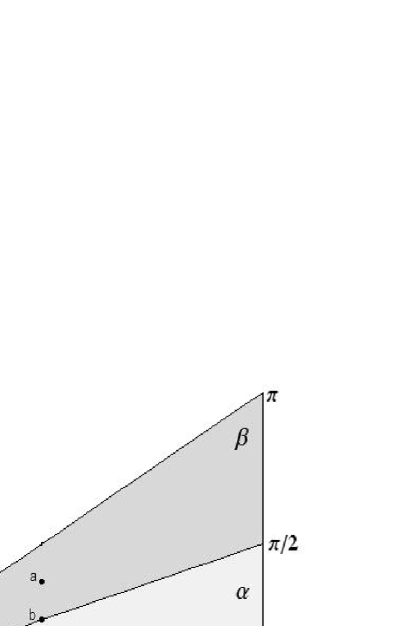
Figure 3: Admissible range of the quantities $\phi_{in}/M_{P}$ and $F/M_{P}$ for dark-energy like axion-field solutions today. The triangular area $\alpha$ ($\beta$) corresponds to $\phi_{in}/M_{P}$ being below (above) the inflexion point of $V(\phi)$. The horizontal line $\phi_{in}/M_{P}=0.278$ indicates a rapid cross-over from slowly rolling to oscillating solutions.

In Fig. 3 admissible ranges for the initial conditions at $t=t_{dec}$ are shown. The triangular area $\alpha$ represents the allowed parameter range for a slowly rolling field at present. The horizontal line $\phi_{in}/M_{P}=0.278$ indicates a rapid crossover from dark-energy-like (above) to oscillating (below) solutions. The allowed range is enlarged by including the trapezoidal area $\beta$ corresponding to a negative curvature of the potential. Notice that for $\pi F/2\leq\phi_{in}\leq\pi F$ there are slowly rolling solutions with the needed amount of present dark energy also for $F/M_{P}<0.177$. However, for a decreasing value of $F/M_{P}$ we observe that $\phi_{in}$ needs to be closer to the maximum $\pi F$ which is somewhat of a fine-tuned situation [5]. We thus pick representative initial conditions as depicted in Fig 3.

In Table 1 we present our numerical results obtained for initial values corresponding to the points (a),(b),(c) and (d) in Fig. 3. The values of the following quantities are determined: $\lambda$ such that $\Omega_{\phi}=0.73$ at present, the present age $t_{0}$ of the universe, the present Zeldovich parameter for the axion fluid alone, $w_{\phi}(t_{0})=(p_{\phi}/\rho_{\phi})_{t=t_{0}}$ (see eq. (16)), and for the entire Universe, $w_{tot}(t_{0})=(p_{tot}/\rho_{tot})_{t=t_{0}}$ and the value of redshift $z_{acc}$ corresponding to the transition between decelerated and accelerated expansion.

Table 1. The values of selected cosmological parameters obtained for variable 1 initial values at CMB decoupling keeping $F/M_{P}=0.5$ fixed.

points in Fig. 3	$\phi_{in}/M_{P}$	$\lambda$	$t_{0}$ (Gy)	$w_{\phi}(t_{0})$	$w_{tot}(t_{0})$	$z_{acc}$
(a)	$3\pi/4$	$22.15$	$13.65$	$-0.97$	$-0.71$	$0.76$
(b)	$\pi/4$	$22.15$	$13.65$	$-0.97$	$-0.71$	$0.76$
(c)	$\pi/6$	$26.96$	$13.56$	$-0.91$	$-0.66$	$0.79$
(d)	$0.328$	$37.27$	$13.08$	$-0.61$	$-0.44$	$0.92$

For the set of initial values (a),(b), and (c) the axion field does not roll until $t_{0},$ as indicated by the quantity $w_{\phi}(t_{0})\simeq-1$. For point (d) $\phi_{in}/M_{P}$ is just above the threshold in (21) causing the field $\phi$ to roll at present: $w_{\phi}(t_{0})=-0.61$. According to ref. [38] $w_{\phi}(t_{0})=-0.61$ is already inconsistent with observation ($w_{\phi}(t_{0})<-0.78$ at 95% C.L.). Decreasing $\phi_{in}/M_{P}$ further one rapidly runs into the regime $w_{tot}(t_{0})>-1/3$ where the present Universe does not accelerate. The values of $z_{acc}$ obtained for (a), (b), and (c) are in approximate agreement with $z_{acc}=0.75$ obtained for a standard $\Lambda$CDM model. Moving $\frac{F}{M_{P}}$ within the allowed range $\alpha\cup\beta$ at fixed values of $\phi_{in}/M_{P}$, see Fig. 3, the values of the cosmological parameters in Tab. 1 are almost unaffected.

Due to the dynamical nature of dark energy in our model the Universe will not run into pure de Sitter expansion in the future as it does for the $\Lambda$CDM model but rather epochs of accelerated and decelerated expansions will alternate: $z_{acc}$ corresponds to the first of many more future turning points ($\overset{\cdot\cdot}{a}=0$). This, however, presumes that the axion-SU(2)${}_{{\tiny\mbox{CMB}}}$ coupling will remain unaffected by the future evolution.

5 A massive photon in the future

Here we consider the future evolution up to the point where SU(2)${}_{{\tiny\mbox{CMB}}}$ undergoes the transition to its preconfining phase. For simplicity we assume that the present age of the Universe $t_{0}$ is given by the time when $T_{0}=T_{{\tiny\mbox{CMB}}}$ is first reached. Because of the discontinuity of the energy density (Fig. 2)

$$\frac{\rho_{c,M}}{T_{{\tiny\mbox{CMB}}}^{4}}-\frac{\rho_{c,E}}{T_{{\tiny\mbox{CMB}}}^{4}}=\frac{4}{3}\frac{\pi^{2}}{30}$$ (22)

the system cannot jump into the preconfining (magnetic) phase where the photon possesses a mass and thus an additional polarization because of condensed monopoles in the ground state. The energy gap $\frac{4}{3}\frac{\pi^{2}}{30}$ is the sum of the energy gap of the photon gas ($=\frac{\pi^{2}}{30}$) and of the ground state ($=\frac{1}{3}\frac{\pi^{2}}{30}$); we refer to the Appendix for the details. Therefore, the system remains in the deconfining (electric) phase in a supercooled state (with its ground state still being an ensemble of interacting calorons instead of monopoles) so long as the energy density of the electric phase $\rho_{E}$ is smaller than the energy density of the magnetic phase $\rho_{M}$ ($\rho_{E}<\rho_{M}$). At a certain value of temperature, $\lambda_{\ast,E}=2\pi T_{\ast}/\Lambda_{E}<\lambda_{c,E}=2\pi T_{c,E}/\Lambda_{E}$, equality $\rho_{E}=\rho_{M}$ takes place. At this point the condensation of monopoles occurs and the photon becomes massive (for $\lambda_{\ast,E}\leq\lambda_{E}\leq\lambda_{c,E}$ monopoles are not sufficiently liberated by the associated large-holonomy calorons to facilitate unlimited mobility).

Figure 4: The situation for the (dimensionless) energy density in the critical region: the dashed line represents the continuation of the energy density of the deconfining phase (solid grey line) for $T<T_{c,E}$ (supercooled state, realized for decreasing temperature, $m_{\gamma}=0$). The solid grey line depicts the energy density in the preconfining phase (realized for increasing temperature, $m_{\gamma}>0$). At the intersection point $\lambda_{E}=\lambda_{\ast,E}$ a phase transition from the supercooled deconfining to the preconfining dynamics occurs.

The situation is depicted in Fig. 4, where the dashed line represents the continuation of the (dimensionless) energy density $\rho_{E}/\Lambda_{E}^{4}$ for $\lambda_{E}<\lambda_{c,E}$. The corresponding analytical expressions are given in the Appendix [12]. The intersection $\rho_{E}/T^{4}=\rho_{M}/T^{4}$ occurs at $\lambda_{\ast,E}=12.15<\lambda_{c,E}=13.87$ (i.e. $T_{\ast}/T_{c,E}=0.88$) (see Fig. 4, for technical details see the Appendix). Driven by cosmological expansion, which essentially is sourced by dark matter and the axion field, the SU(2)${}_{{\tiny\mbox{CMB}}}$ thermodynamics evolves into a supercooled state (deconfining phase) according to eq. (12) ($i=$ CMB) down to the point where the density $\rho_{\ast}$ (i.e. the transition temperature $T_{\ast}$) is reached. The numerical result for the scale factor at $T=T_{\ast}$ is $a(t_{\ast})/a_{0}=1.17.$ At this point the photon acquires a Meissner mass. Notice that according to eq. (2) the anomaly-mediated decay width $\Gamma_{\phi\rightarrow 2\gamma}$ of the axion into two photons is much smaller than the present Hubble parameter $H_{0}$:

$$\Gamma_{\phi\rightarrow 2\gamma}<\left(\frac{m_{\phi}}{F}\right)^{2}\,m_{\phi}\,\,\sim 10^{-155}\text{ eV}\lll H_{0}\sim 10^{-33}\text{ eV.}$$ (23)

Thus it is justified to treat the axion as a coherent field for any practical purpose and to consider the axion and the SU(2)${}_{{\tiny\mbox{CMB}}}$ fluids to be separately conserved as in eq. (12).

The numerical value of the time interval $\Delta t_{m_{\gamma}=0}=t_{*,E}-t_{0}$ follows from future cosmology according to eq. (11). For the sets of initial values (a)–(d) in Tab. 1 we obtain the following numbers:

$$(a) \ \ \Delta t_{m_{\gamma}=0}=2.20\,\mbox{Gy}\,,\ \ \ \ \ (b)\ \ \Delta t_{m_{\gamma}=0}=2.20\,\mbox{Gy}\,,$$

$$(c) \ \ \Delta t_{m_{\gamma}=0}=2.22\,\mbox{Gy}\,,\ \ \ \ \ (d)\ \ \Delta t_{m_{\gamma}=0}=2.29\,\mbox{Gy}\,.$$ (24)

The value $\Delta t_{m_{\gamma}=0}\simeq$ 2.2 Gy depends only weakly on the chosen parameter set. The error in determining the quantity $\Delta t_{m_{\gamma}=0}$ is dominated by the observational uncertainty for the present Hubble parameter $H_{0}$. According to [38] we have $\frac{\delta H(t_{0})}{H(t_{0})}\sim\pm 0.056$. We have run our simulations with the upper (lower) limit for the error range. This generates a decrease (increase) for $\Delta t_{m_{\gamma}=0}$ of about 0.15 Gy.

Throughout the work we assumed that the temperature $T_{c,E}=T_{{\tiny\mbox{CMB}}}$ is reached today. However, the photon is massless and unscreened in the entire range $T_{\ast}$ $\leq T\leq T_{c,E}$. Therefore the present CMB-temperature could also be below $T_{c,E}$. As a consequence, the quantity $\Delta t_{m_{\gamma}=0}$ represents an upper bound for the time interval between the present and the occurrence of the phase transition.

The existence of extra-galactic magnetic fields [40, 41] could indeed signal the onset of a superconducting vacuum. Possibly, a quantitative analysis would rely on tunneling effects connecting the two trajectories in Fig. 4. Such an unconventional interpretation of extra-galactic magnetic fields needs future investigation.

6 Summary and Conclusions

We have elaborated on the idea that the present density of dark energy arises from an ultra-light axion field with Peccei-Quinn scale comparable to $M_{P}$ [1]. More precisely, we have linked the normalization $\mu^{4}$ of the axion potential in eq. (1) to the existence of an SU(2) Yang-Mills theory of scale $\Lambda_{{\tiny\mbox{CMB}}}\sim\mu$ comparable to the temperature $T_{{\tiny\mbox{CMB}}}$ of the present cosmic microwave background. Such an assertion has its justification in nonperturbative results obtained recently for SU(2) Yang-Mills thermodynamics [12]. As a result, we have obtained an upper bound $\Delta t_{m_{\gamma}=0}\simeq 2$ Gy for the length of the time interval from the present to the phase transition where the photon acquires a Meissner mass.

Throughout our work we have assumed a cold dark matter component $\rho_{M}=0.23\,\rho_{c}$ of unknown origin at present. (A possibility would be that $\rho_{M}$ arises due to the decay of one or more oscillating, coherent axion fields $\phi_{i}$ with $F_{i}\ll M_{P}$ into their particles at earlier epochs.) A more unified but also more speculative picture would arise if today’s rolling axion field would describe both dark matter and dark energy, see [42] and refs. therein. On the one hand, according to our simulations (performed with a canonical kinetic term) such a scenario would imply an age of the Universe of about 20 Gy as opposed to 13.7 Gy with conventional cold dark matter. Also one would obtain $z_{acc}\sim 3$ as opposed to $z_{acc}\sim 0.75$, possibly endangering structure formation. On the other hand, structure formation and the flattening of the rotation curves of galaxies would need an explanation in terms of ripples and lumps of a coherent axion field [43]. Moreover, the relation between luminosity distance and redshift as observed from SNe Ia standard candles would have to be postdicted with a pressureless contribution to the Hubble parameter that acquired nominal strength only very recently. The future will tell (gravitational lensing signatures for galaxies, theoretical results on the stability of the system axion-lump plus baryonic matter plus gravity) whether such a possibility is viable.

For completeness we have investigated how the latter scenario affects our estimate $\Delta t_{m_{\gamma}=0}$. By defining the quantity $\eta$ through $\eta=-p_{\phi}$ and $\rho_{\phi}=\dot{\phi}^{2}+\eta$ the axion fluid can be split into a component with $\rho_{\Lambda}=\eta$ (with $w_{\Lambda}=-1$) and a component $\rho_{DM}=\dot{\phi}^{2}$ (with $w_{DM}=0$). Notice that the so defined components are not separately conserved. The task is to uniquely fix $\phi_{in}$ and $\lambda$ in eq. (14) such that $\Omega_{\phi}=0.96$ today (with $\Omega_{{\tiny\mbox{Baryon}}}=0.04)$) and such that $\Omega_{\Lambda}=0.73$ and $\Omega_{DM}=0.23$. Using $\frac{F}{M_{P}}=0.5$ we obtain $\frac{\phi_{in}}{M_{P}}=0.53$ and $\lambda=31.9$. This yields $\Delta t_{m_{\gamma}=0}=2.21\,$Gy. Thus our estimate $\Delta t_{m_{\gamma}=0}$ is rather model independent.

Finally, let us make a few comments concerning future activity. The postulate SU(2)${}_{{\tiny\mbox{CMB}}}\overset{{\tiny\mbox{today}}}{=}$U(1)_Y entails consequences for the CMB map of fluctuations in temperature and in electric/magnetic field polarization at large angles [15, 13]. To analyze these effects more quantitatively needs precise information on the underlying cosmology; this basic step was addressed in the present work.

For the viability of the postulate SU(2)${}_{{\tiny\mbox{CMB}}}\overset{{\tiny\mbox{today}}}{=}$U(1)_Y an alternative interpretation of electroweak SM physics in terms of underlying, nonperturbative and pure Yang-Mills dynamics is necessary. Although we have checked a few experimental benchmarks on this scenario further theoretical work surely is needed.

Appendix A Expressions for the energy density and the pressure

We start from the effective Lagrangians in the deconfining and preconfining phases as described in [12] and we briefly derive in a self-contained way the corresponding 1-loop thermodynamical quantities. Higher order loop corrections turn out to be of the order 0.1% [13], thus are irrelevant for our cosmological application.
Deconfining (electric) phase:
(Occurs for $T>T_{c,E}=\Lambda_{E}\lambda_{c,E}/2\pi$, $\lambda_{c,E}=13.87$, $\Lambda_{E}$ the Yang-Mills scale in electric phase).
The effective Lagrangian for the description of SU(2)-Yang-Mills thermodynamics in the deconfining phase and in the unitary gauge reads [12]:

$$\mathcal{L}_{{\tiny\mbox{dec-eff}}}^{u.g.}=\frac{1}{4}\left(G_{E}^{a,\mu\nu}[a_{\mu}]\right)^{2}+2e(T)^{2}\left|\varphi_{E}\right|^{2}\left(\left(a_{\mu}^{(1)}\right)^{2}+\left(a_{\mu}^{(2)}\right)^{2}\right)+\frac{2\Lambda_{E}^{6}}{\left|\varphi_{E}\right|^{2}}\,,$$ (25)

where $G_{E,\mu\nu}^{a}=\partial_{\mu}(a_{\nu}^{a})-\partial_{\nu}(a_{\mu}^{a})+e\varepsilon^{abc}a_{\mu}^{b}a_{\nu}^{c}$ is the SU(2) stress-energy tensor for the topologically trivial fluctuations $a_{\mu}^{a}$ (with effective coupling $e=e(T)$) and the adjoint scalar background-field $\varphi_{E}$ embodies the spatial coarse graining of caloron and anticaloron field configurations (see [12] for a microscopic derivation, see [44] for a macroscopic one). The quantum fluctuations $a_{\mu}^{(1,2)},$ in our work identified by $V^{\pm},$ are massive, while the gauge mode $a_{\mu}^{(3)},$ here the photon, stays massless (spontaneous symmetry breaking $SU(2)\rightarrow U(1)$). The mass of $V^{\pm}$ reads explicitly (see (25)):

$$m=m_{V^{+}}=m_{V^{-}}=2e(T)\left|\varphi_{E}\right|;\text{ }\left|\varphi_{E}\right|=\sqrt{\frac{\Lambda_{E}^{3}}{2\pi T}}\,.$$ (26)

At this stage the effective running coupling $e=e(T)$ is not yet known. Its behavior is determined by imposing the thermodynamical self-consistency, see below.

The energy density and the pressure are the sum of three terms,

$$\rho_{E}=\rho_{E,\gamma}+\rho_{E,V^{\pm}}+\rho_{E,gs},\text{ }p_{E}=p_{E,\gamma}+p_{E,V^{\pm}}+p_{E,gs}\,,$$ (27)

corresponding to the contributions of the massless gauge mode $\gamma$, the two massive gauge modes $V^{\pm}$ and the ground state, respectively. The 1-loop expressions are easily obtained from the effective Lagrangian (25):

$$\rho_{E,\gamma}=2\frac{\pi^{2}}{30}\,T^{4},\text{ }\rho_{E,V^{\pm}}=6\int_{0}^{\infty}\frac{k^{2}dk}{2\pi^{2}}\frac{\sqrt{m^{2}+k^{2}}}{\exp(\frac{\sqrt{m^{2}+k^{2}}}{T})-1},\text{ }\rho_{E,gs}=4\pi\Lambda_{E}^{3}T\,$$ (28)

$$p_{E,\gamma}=2\frac{\pi^{2}}{90}T^{4},\text{ }p_{E,V^{\pm}}=-6\,T\int_{0}^{\infty}\frac{k^{2}dk}{2\pi^{2}}\ln\left(1-e^{-\frac{\sqrt{m^{2}+k^{2}}}{T}}\right),\text{ }p_{E,gs}=-\rho_{E,gs}\,.$$ (29)

We first rewrite the system in terms of dimensionless quantities:

$$\overline{\rho}_{E}=\frac{\rho_{E}}{T^{4}},\text{ }\overline{p}_{E}=\frac{p_{E}}{T^{4}},\text{ }\lambda=\lambda_{E}=\frac{2\pi T}{\Lambda_{E}},\text{ }a(\lambda)=\frac{m(T)}{T}=2\frac{e(T)}{T}\left|\varphi_{E}\right|$$ (30)

where the function $a=a(\lambda)$ has been introduced for later use.

The dimensionless density and pressure, expressed as functions of the dimensionless temperature $\lambda$, read:

$$\overline{\rho}_{E,\gamma}=2\frac{\pi^{2}}{30},\text{ }\overline{\rho}_{E,V^{\pm}}=\frac{3}{\pi^{2}}\int_{0}^{\infty}dx\frac{x^{2}\sqrt{x^{2}+a^{2}}}{e^{\sqrt{x^{2}+a^{2}}}-1},\text{ }\overline{\rho}_{E,gs}=\frac{2(2\pi)^{4}}{\lambda^{3}}\,.$$ (31)

$$\overline{p}_{E,\gamma}=2\frac{\pi^{2}}{90},\text{ }\overline{p}_{E,V^{\pm}}=-\frac{3}{\pi^{2}}\int_{0}^{\infty}x^{2}dx\ln\left(1-e^{-\sqrt{x^{2}+a^{2}}}\right),\text{ }\overline{p}_{E,gs}=-\text{ }\overline{\rho}_{E,gs}\,.$$ (32)

We impose the validity of the thermodynamical Legendre transformation

$$\rho=T\frac{dP}{dT}-P\iff\overline{\rho}=\lambda\frac{d\overline{p}}{d\lambda}+3\overline{p}$$ (33)

(expressed with both dimensional and dimensionless functions). By substituting the expressions (31), (32) into (33) we determine the following differential equation for $a=a(\lambda)$:

$$1 = -\frac{6\lambda^{3}}{(2\pi)^{6}}\left(\lambda\frac{da}{d\lambda}+a\right)aD(a),\text{ }$$ (34)

$$D(a) = \int_{0}^{\infty}dx\frac{x^{2}}{\sqrt{x^{2}+a^{2}}}\frac{1}{e^{\sqrt{x^{2}+a^{2}}}-1},\text{ }a(\lambda_{in})=0.$$ (35)

For sufficiently large initial value $\lambda_{in}$ the solution for $a(\lambda)$ is independent on $\lambda_{in}$: a low-temperature attractor with a logarithmic pole at $\lambda_{c,E}=$ $13.87$ is seen (infinite mass for $V^{\pm}$ leading to their thermodynamical decoupling). The effective coupling is given by $e=e(\lambda)=a(\lambda)\lambda^{3/2}/4\pi$ and shows a plateaux at $e\sim 8.89$, see Fig. 1.

Once the function $a=a(\lambda)$ is determined, density and pressure in the deconfining phase are numerically obtained and are plotted in Fig. 2.
Preconfining (magnetic) phase:
(Occurs for $11.57\,\Lambda_{E}/2\pi=T_{c,M}\leq T\leq T_{c,E}=\Lambda_{E}\lambda_{c,E}/2\pi$).

The effective Lagrangian for the description of SU(2)-Yang-Mills thermodynamics in the preconfining phase and in the unitary gauge reads [12]:

$$\mathcal{L}_{{\tiny\mbox{prec-eff}}}^{u.g.}=\frac{1}{4}(F_{E}^{\mu\nu})^{2}+\frac{1}{2}g^{2}\left|\varphi_{M}\right|^{2}(a_{\mu}^{(3)})^{2}+\frac{2\Lambda_{M}^{6}}{\left|\varphi_{M}\right|^{2}},\text{ }$$ (36)

where $F_{E}^{\mu\nu}=\partial_{\mu}a_{\nu}^{(3)}-\partial_{\nu}a_{\mu}^{(3)}$ is the (dual) abelian stress-energy tensor, the complex scalar field $\varphi_{M}$ describes the condensate of magnetic monopoles, and $\Lambda_{M}$ the Yang-Mills scale in the magnetic phase. The remaining $U(1)$ symmetry of the deconfining phase is broken. The photon acquires a temperature dependent mass:

$$m_{\gamma}=g\left|\varphi_{M}\right|=bT\,,\text{ }\left|\varphi_{M}\right|=\sqrt{\frac{\Lambda_{M}^{3}}{2\pi T}}$$ (37)

where the function $b\equiv b(\lambda)$ is introduced for later use. The effective coupling $g\equiv g(\lambda)$ is not yet known. As before, thermodynamical self-consistency will determine its behavior.

The energy density and the pressure are now the sum of two terms referring to the photon and to the ground state respectively:

$$\rho_{M}=\rho_{M,\gamma}+\rho_{M,gs},\text{ }p_{M}=p_{M,\gamma}+p_{M,gs},$$ (38)

with:

$$\rho_{M,\gamma} = 3\int_{0}^{\infty}\frac{k^{2}dk}{2\pi^{2}}\frac{\sqrt{m_{\gamma}^{2}+k^{2}}}{\exp(\frac{\sqrt{m_{\gamma}^{2}+k^{2}}}{T})-1},\text{ }\rho_{M,gs}=4\pi\Lambda_{M}^{3}T$$ (39)

$$p_{M,\gamma} = -3\,T\int_{0}^{\infty}\frac{k^{2}dk}{2\pi^{2}}\ln\left(1-e^{-\frac{\sqrt{m_{\gamma}^{2}+k^{2}}}{T}}\right),\text{ }p_{M,gs}=-\rho_{M,gs}\,.$$ (40)

The corresponding dimensionless quantities are expressed in terms of $\lambda=2\pi T/\Lambda_{E}$ and read:

$$\overline{\rho}_{M,\gamma} = \frac{3}{2\pi^{2}}\int_{0}^{\infty}dx\frac{x^{2}\sqrt{x^{2}+b^{2}}}{e^{\sqrt{x^{2}+b^{2}}}-1},\text{ }\overline{\rho}_{M,gs}=\left(\frac{\Lambda_{M}}{\Lambda_{E}}\right)^{3}\frac{2(2\pi)^{4}}{\lambda^{3}}$$ (41)

$$\overline{p}_{M,\gamma} = -\frac{3}{2\pi^{2}}\int_{0}^{\infty}x^{2}dx\ln\left(1-e^{-\sqrt{x^{2}+b^{2}}}\right),\text{ }\overline{p}_{M,gs}=-\text{ }\overline{\rho}_{M,gs}\,.$$ (42)

The ratio $\Lambda_{M}/\Lambda_{E}$ is determined by imposing that the pressure and the photon mass are continuous functions across the phase transition at $\lambda_{c,E}=$ $13.87$ (second order phase transition, see [12]). A continuous photon mass requires $b(\lambda\rightarrow\lambda_{c,E}^{-})=0.$ Thus, by equating eq. (32) and eq. (42), we obtain the following matching condition:

$$\left(\frac{\Lambda_{M}}{\Lambda_{E}}\right)^{3}=1+\frac{\lambda_{c,E}^{3}}{720(2\pi)^{2}}=1.09\,.$$ (43)

As a consequence, the energy-gap at the phase transition reads:

$$\Delta=\overline{\rho}_{M}(\lambda_{c,E})-\overline{\rho}_{E}(\lambda_{c,E})=\frac{4}{3}\frac{\pi^{2}}{30}\,.$$ (44)

We require thermodynamical self-consistency in the magnetic phase: By substituting the expressions (41), (42) into eq. (33) we obtain the following differential equation for $b=b(\lambda)$:

$$1=-\frac{3\lambda^{3}}{(2\pi)^{6}}\left(\frac{\Lambda_{E}}{\Lambda_{M}}\right)^{3}\left(\lambda\frac{db}{d\lambda}+b\right)bD(b),\text{ }b(\lambda=\lambda_{c,E})=0\,.$$ (45)

The behavior of the magnetic coupling $g(\lambda)=b(\lambda)\lambda^{3/2}/4\pi$ is shown in Fig. 1. A pole at the critical value $T_{c,M}=11.57\Lambda_{E}/2\pi$ is encountered. At this temperature the photon mass diverges. For temperature smaller than $T_{c,M}$ the system is in a completely confining phase.
Supercooled electric phase:
(Occurs for $\Lambda_{E}\lambda_{\ast c,M}/2\pi=T_{\ast}\leq T\leq T_{c,E}=\Lambda_{E}\lambda_{c,E}/2\pi,$ $\lambda_{\ast}=12.15$)

The system cooling down from the deconfining into the preconfining phase stays in a supercooled deconfining phase by virtue of the energy gap. Energy density and pressure in the supercooled deconfining phase are given as:

$$\overline{\rho}_{E}^{s.c.}=\overline{\rho}_{E,\gamma}^{s.c.}+\overline{\rho}_{E,gs},\text{ }\overline{p}_{E}^{s.c.}=\overline{p}_{E,\gamma}^{s.c.}+\overline{p}_{E,gs}^{s.c.}\ \ \ \ \ \mbox{where}$$ (46)

$$\overline{\rho}_{E,\gamma}^{s.c.}=2\frac{\pi^{2}}{30}\,,\ \ \text{ }\overline{\rho}_{E,gs}=\frac{2(2\pi)^{4}}{\lambda^{3}}\,;\ \ \ \ \text{ }\overline{p}_{E,\gamma}^{s.c.}=2\frac{\pi^{2}}{90}\,,\ \ \text{ }\overline{p}_{E,gs}^{s.c.}=-\text{ }\overline{\rho}_{E,gs}\,.$$ (47)

The behavior of $\overline{\rho}_{E}^{s.c.}$ and $\overline{\rho}_{M}$ is indicated in Fig. 4 where the corresponding transition value $\lambda_{\ast}$ ($\overline{\rho}_{E}^{s.c.}(\lambda_{\ast})=\overline{\rho}_{M}(\lambda_{\ast})$) is determined as $\lambda_{\ast}=12.15$.

References

- [1] J. A. Frieman, C. T. Hill, A. Stebbins, and I. Waga, Phys. Rev. Lett. 75, 2077 (1995).
- [2] J. E. Kim and H.-P. Nilles, Phys. Lett. B 553, 1 (2003).
- [3] F. Wilczek, hep-ph/0408167.
- [4] L. J. Hall, Y. Nomura, and S. J. Oliver, Phys. Rev. Lett. 95, 141302 (2005).
- [5] N. Kaloper and L. Sorbo, hep-ph/0511543.
- [6] R. Barbieri, L. J. Hall, S. J. Oliver and A. Strumia, Phys. Lett. B 625 (2005) 189 [arXiv:hep-ph/0505124]
-
[7]
R. D. Peccei and H. R. Quinn, Phys. Rev. D 16, 1791 (1977).
R. D. Peccei and H. R. Quinn, Phys. Rev. Lett. 38, 1440 (1977). - [8] J. E. Kim, arXiv:hep-ph/0308081.
- [9] A. G. Riess et al., Astron. J. 116, 1009 (1998).
- [10] S. Perlmutter et al., Astrophys. J. 483, 565 (1998).
- [11] B. P. Schmidt et al., Astrophys. J. 507, 46 (1998).
- [12] R. Hofmann, Int. J. Mod. Phys. A 20, 4123
- [13] U. Herbst, R. Hofmann, and J. Rohrer, Act. Phys. Pol. B 36, 881 (2005).
- [14] R. Hofmann, talk given at 29th John’s Hopkins Workshop on Theoretical Physics, Budapest 2005, hep-ph/0508176.
-
[15]
M. Schwarz, R. Hofmann, and F. Giacosa, hep-th/0603078.
M. Schwarz, R. Hofmann, and F. Giacosa, hep-ph/0603174. -
[16]
C. P. Korthals Altes, hep-ph/0406138, hep-ph/0408301.
C. P. Korthals Altes, Acta Phys. Polon. B 34, 5825 (2003).
P. Giovannangeli and C. P. Korthals Altes, Nucl. Phys. B 608, 203 (2001).
C. Korthals-Altes, A. Kovner, and M. A. Stephanov, Phys. Lett. B 469, 205 (1999). - [17] Ch. Hoelbing, C. Rebbi, and V. A. Rubakov, Phys. Rev. D 63, 034506 (2001).
- [18] R. Hofmann, hep-th/0609033.
- [19] F. R. Brown et al., Phys. Rev. Lett. 61, 2058 (1988).
- [20] Y. Deng, in BATAVIA 1988, proc. LATTICE 88, 334.
- [21] K. Langfeld, E. M. Ilgenfritz, H. Reinhardt and G. Shin, Nucl. Phys. Proc. Suppl. 106 501 (2002)[arXiv:hep-lat/0110024].
- [22] E. Braaten and R. D. Pisarski, Nucl. Phys. B 337, 569 (1990).
- [23] U. Herbst and R. Hofmann, hep-th/0411214.
-
[24]
D. F. Litim and J. M. Pawlowski, in The Exact
Renormalization Group, eds. Krasnitz et al., World Scientific, 168 (1999)
[hep-ph/9811272].
D. F. Litim and J. M. Pawlowski, hep-th/0609122. -
[25]
M. D’Attanasio and M. Pietroni, Nucl. Phys. B 498, 443 (1997).
D. Comelli and M. Pietroni, Phys. Lett. B 417, 337 (1998). - [26] J. Braun and H. Gies, JHEP 0606, 024 (2006).
- [27] P. J. Peebles and D. T. Wilkinson, Phys. Rev. 174, 2168 (1968).
- [28] R. H. Cybert et al., Astropart. Phys. 23, 313 (2005).
- [29] H. V. Klapdor-Kleingrothaus, I. V. Krivosheina, A. Dietz, and O. Chkvorets, Phys. Lett. B 586, 198 (2004).
- [30] O. Manuel, in proc. Fourth Intern. Conf. on Beyond Standard Model Physics 2003, astro-ph/0411658.
- [31] see http://www.iter.org/ and publications therein.
- [32] K. Choi and A. Santamaria, Phys. Rev. D 42, 293 (1990).
- [33] H. T. Janka, K. Kifonidis and M. Rampp, Lect. Notes Phys. 578 (2001) 333 [arXiv:astro-ph/0103015].
- [34] A. Burrows and T. A. Thompson, Report,” arXiv:astro-ph/0210212.
- [35] L. Scheck, K. Kifonidis, H. T. Janka and E. Mueller, arXiv:astro-ph/0601302 and refs. therein.
- [36] R. Fariello, H. Forkel, and G. Krein, Phys. Rev. D 72, 105015 (2005).
-
[37]
P. A. M. Dirac, Proc. Roy. Soc. (London), A 133, 60
(1931),
J. Schwinger, Phys. Rev. 144, 1087 (1966),
D. Zwanziger, Phys. Rev. 176, 1489 (1968),
N. Cabibbo and E. Ferrari, Nuovo Cimento 23 1147 (1962). -
[38]
S. Eidelman et al., Phys. Lett. B 592, 1 (2004).
D. N. Spergel et al., Astrophys. J. Suppl. 148, 175 (2003). - [39] E. R. Williams, J. E. Faller, and H. A. Hill, Phys. Rev. Lett. 26, 721 (1971).
- [40] Z. G. Dai et al., Astrophys. J. 580, L7 (2002).
- [41] J. Bagchi et al., New Astron. 7, 249 (2002).
- [42] T. Padmanabhan, Phys. Rept. 380 (2003) 235 [arXiv:hep-th/0212290].
- [43] C. Wetterich, Phys. Lett. B 522, 5 (2001).
- [44] F. Giacosa and R. Hofmann, arXiv:hep-th/0609172.