Anti-de Sitter boundary in Poincaré coordinates

Abstract

We build up a detailed description of the space-time boundary of a Poincaré patch of anti-de Sitter ($AdS$) space. We map the Poincaré $AdS$ boundary to the global coordinate chart and show why this boundary is not equivalent to the global $AdS$ boundary. The Poincaré $AdS$ boundary is shown to contain points of the bulk of the entire $AdS$ space. The Euclidean $AdS$ space is also discussed. In this case one can define a semi-global chart that divides the $AdS$ space in the same way as the corresponding Euclidean Poincaré chart.

I Introduction

Some years ago, Maldacena found very important dualities between string theories and conformal field theories (CFT) known collectively as $AdS$/CFT correspondence Maldacena:1997re ; Petersen:1999zh ; Aharony ; D'Hoker:2002aw . A particularly important example relates string theory in a ten dimensional curved space with super-conformal Yang Mills theory in four dimensional flat space. The starting point for finding this duality was a solution of low energy string theory containing D3-brane charge. The corresponding metric, studied in HS , is similar to that of a black hole. The near horizon limit of this D3-brane metric corresponds to the direct product of a Poincaré chart of $AdS_{5}\,$ space and a compact $S^{5}$ space. String theory in this ten dimensional space, referred for short, as $AdS_{5}\times S^{5}\,$ is dual to the four dimensional CFT. As we will see in detail, a Poincaré chart represents only a region of the entire $AdS$ space. Since this distinction will be important here, we will call this region as: Poincaré $AdS$ space.

Quantization of fields in global $AdS$ space requires the introduction of a boundary, at spatial infinity, where vanishing flux conditions can be imposed. Otherwise particles could enter or leave the space in finite times Avis:1977yn ; Breitenlohner:1982bm . This boundary has the topology of $S^{1}\times S^{n-1}\,$. The boundary of a Poincaré $AdS$ space is a different region. This boundary assumes a special role in the $AdS$/CFT correspondence. It was shown in m3 ; Witten:1998qj that correlation functions for the CFT can be calculated in terms of string theory in such a way that the CFT is interpreted as living on the boundary of the Poincaré $AdS$ space. So, we can think of the $AdS$/CFT correspondence as a realization of the holographic principle HOL1 ; HOL2 since it relates a theory in a space with gravity to a theory on its boundary. It is important to remark that although the $AdS$/CFT correspondence was originally formulated for a Poincaré AdS space, it also holds for $AdS$ space in global coordinatesAharony . Previous related discussions of the $AdS$ boundary can be found in Witten2 ; Boschi-Filho:2001gr . Field quantization in Poincaré $AdS$ space were discussed for example in Balasubramanian:1998sn ; Boschi-Filho:2000vd .

The AdS /CFT prescription for relating bulk and boundary theories is Witten:1998qj

$$exp\Big{(}-S(\phi)\,\Big{)}\,=\,\langle exp\int\phi_{0}{\cal O}\,\rangle$$ (1)

where $S(\phi)$ is the on shell action for the bulk field $\phi$ and $\phi_{0}$ is proportional to the boundary value of $\phi$. This $\phi_{0}$ plays the role of an external source for the boundary conformal operators ${\cal O}$. Using this equation one can calculate the conformal correlation functions.

In order to calculate correlation functions one must choose a coordinate system for the AdS space. This choice has non trivial consequences. As discussed in detail in ref Emparan:1999pm , for the Euclidean case, different coordinate charts of AdS space can lead to different boundaries. Depending on the choice of metric, spaces that are locally equivalent to $AdS_{n+1}\,$ can have boundaries like, for example, $\rm l\!R\,^{n}\,,\,S^{1}\times S^{n-1}\,,\,S^{1}\times\rm l\!R\,^{n-1}\,,\,S^{1}\times H^{n-1}\,$. The different metrics representing AdS space are related by diffeomorphisms (coordinate transformations) plus the inclusion of points at infinity and some identifications. From equation (1), where the on shell action is a boundary term, we see that the dual conformal field theories are defined in different spaces, depending on the choice of the AdS metric. These theories will in general have different energies as shown in Emparan:1999pm . The difference in mass in global and Poincaré coordinates is also discussed for example in Balasubramanian:1999re .

Another example of the non trivial role of the choice of AdS coordinate systems is the case of the stress tensor. For asymptotically AdS spaces one can use the AdS/CFT correspondence to relate a gravitational stress tensor to the expectation value of the corresponding conformal stress tensorBalasubramanian:1999re . This boundary tensor diverges but can be regularized adding counterterms to the action. This subtraction procedure depends on the geometry of the boundary. Different metrics will lead to different expectation values of the conformal stress tensor (see also, for example, Astefanesei:2004kn ). The choice of coordinate system can also change the stability of the AdS space when one consider AdS/CFT at finite temperatureWitten:1998zw . For global coordinates, there is phase transition to a black hole geometry at some critical temperature. For Poincaré coordinates there is no thermal phase transition.

In this work, we will begin describing how the Poincaré $AdS$ space arises from a non-trivial change of coordinates for the entire $AdS$ space. Then we will present a division of the Poincaré $AdS$ boundary into regions for which we find well defined mappings to global coordinates. This way the Poincaré $AdS$ boundary will be completely described in the global chart.

II Global and Poincaré coordinates for the Anti-de Sitter space

Anti-de-Sitter space in $n+1$ dimensions can be represented as a hyperboloid of radius $R$

$${X_{0}}^{2}+{X_{n+1}}^{2}-\sum_{i=1}^{n}{{X_{i}}^{2}}=R^{2}\,,$$ (2)

embedded in an n+2 dimensional flat space with metric

$$ds^{2}=-dX_{0}^{2}-dX_{n+1}^{2}+\sum_{i=1}^{n}{{dX_{i}}^{2}}\,.$$ (3)

The coordinates $X_{a}$   for $a=0,..,n+1$ are known as embedding coordinates. We can solve eq. (2) by introducing the following relations

$$X_{0} = R\sec{\rho}\cos{\tau}\,,$$

$$X_{i} = R\,\tan{\rho}\,\Omega_{i}\,,\hskip 28.45274pti=1,..,n\,,$$

$$X_{n+1} = R\sec{\rho}\sin{\tau}\,,$$ (4)

where $0\leq\rho<\pi/2\,$, $\,-\pi<\tau\leq\pi\,$ and $-1\leq\Omega_{i}\leq 1\,$. Coordinates $\rho\,,\tau\,$ and $\Omega_{i}$ represent all the hyperboloid and are called global coordinates. The $\Omega_{i}$ are not independent. They must satisfy the constraint $\,\sum_{i=1}^{n}{{\Omega_{i}}^{2}}=1\,$. The $AdS$ metric in terms of these coordinates reads

$$ds^{2}=\frac{R^{2}}{\cos^{2}\rho}(-d\tau^{2}+d\rho^{2}+\sin^{2}\rho\sum_{i=1}^{n}{(d\Omega_{i})^{2}})\,.$$ (5)

In these global coordinates the $AdS$ boundary is the hypersurface $\rho=\pi/2\,$. This corresponds, in embedding coordinates, to the spatial infinity. So, we can compactify the $AdS$ space by changing the range of the radial coordinate $\rho\,$ to: $0\leq\rho\leq\pi/2$.

On the other hand, the Poincaré coordinate system can be introduced by first defining the light cone coordinates :

$$u \equiv \frac{(X_{0}-X_{n})}{R^{2}}\,,$$

$$v \equiv \frac{(X_{0}+X_{n})}{R^{2}}\,.$$ (6)

This change of coordinates will make it possible to absorb the time-like coordinates $X_{0}$. Redefining the other coordinates as

$$x^{i} \equiv \frac{X_{i}}{Ru}\,\,\,\,\,\,\,\,\,\hskip 28.45274pt\hbox{(space-like)}\,,$$

$$t \equiv \frac{X_{n+1}}{Ru}\,\,\,\,\hskip 28.45274pt\hbox{(time-like)}\,,$$ (7)

equation (2) for the hyperboloid takes the form

$$R^{4}uv+R^{2}u^{2}(t^{2}-{\overline{x}}^{2})=R^{2}\,,$$ (8)

where ${\overline{x}}^{2}\equiv\sum_{i=1}^{n-1}(x^{i})^{2}$. From this equation we can express $v$ in terms of $u\,,t\,,$ and $x^{i}\,$ and find from (6) and (7)

$$X_{0} = \frac{1}{2u}(1+u^{2}(R^{2}+{\overline{x}}^{2}-t^{2}))\,,$$

$$X_{n} = \frac{1}{2u}(1+u^{2}(-R^{2}+{\overline{x}}^{2}-t^{2}))\,,$$

$$X_{i} = Rux^{i}\hskip 28.45274pti=1,..,n-1\,,$$

$$X_{n+1} = Rut\,.$$ (9)

It is useful to change to the coordinate $z\equiv\frac{1}{u}$. This way the Poincaré coordinates $z,\overline{x},t$ are defined by the following relations

$$X_{0} = \frac{1}{2z}(z^{2}+R^{2}+{\overline{x}}^{2}-t^{2})\,,$$

$$X_{i} = \frac{Rx^{i}}{z}\,,\hskip 28.45274pti=1,..,n-1\,,$$

$$X_{n} = \frac{1}{2z}(z^{2}-R^{2}+{\overline{x}}^{2}-t^{2})\,,$$

$$X_{n+1} = \frac{Rt}{z}\,.$$ (10)

The $AdS$ metric in terms of these coordinates takes the nice form

$$ds^{2}=\frac{R^{2}}{z^{2}}(dz^{2}+(d\overline{x})^{2}-dt^{2})\,.$$ (11)

The coordinate $z$ behaves as a radial coordinate and divide the $AdS$ space in two regions. Noting from (6) that

$$\frac{1}{z}\,=\,u=\frac{(X_{0}-X_{n})}{R^{2}}\,,$$ (12)

we conclude that we have two different Poincaré charts. The first chart is the region $z>0$ , that means $X_{0}>X_{n}$ and corresponds to one half of the hyperboloid. In global coordinates this region can be obtained by imposing the condition $\cos{\tau}>\Omega_{n}\sin{\rho}$. The other half of the hyperboloid $X_{0}<X_{n}$ corresponds to the second Poincaré chart, i.e, the region $z<0$   ( in global coordinates the condition is $\cos{\tau}<\Omega_{n}\sin{\rho}$). The Poincaré $AdS$ space is the region of the entire $AdS$ corresponding to one of these two charts (the $z>0$ is usually chosen). Equation (12) shows us that the region $z=0$ does not belong to the $AdS$ space. As we will see, it is part of the $AdS$ boundary.

The hyperplane $X_{0}\,=\,X_{n}$, that cuts the $AdS$ space into the two Poincaré charts, is not contained in these charts but rather corresponds to the limits $z\to\pm\infty$ (or $u=0$). We can see in Figure 1 how the hyperplane $X_{0}\,=\,X_{n}$ cuts the entire $AdS$ space. In this figure we consider the coordinates $X_{i}\,$ ($i=1,..,n-1$) fixed. In this case the region $X_{0}\,=\,X_{n}$ is a plane that intersects the hyperboloid in two straight lines.

There are points of the hyperboloid contained in the cutting hyperplane. From (10) we note that these points require also the condition $t\to\pm\infty$ in order to satisfy (2). In global coordinates these points must satisfy the condition

$$\cos{\tau}\,=\,\Omega_{n}\sin{\rho}\,,$$ (13)

where $0\leq\rho<\pi/2$. It is interesting to analyze the limit $\rho\to\pi/2$, which means: going to spatial infinity. Equation (13) reduces to $\cos{\tau}=\Omega_{n}$ in this limit. This condition is very special because it can be obtained also for z finite. This happens because $\,\cos{\tau}-\Omega_{n}\,\to\,0\,$ when $\rho\to\pi/2$ with $\,0\,<|z|\,<\infty\,$. All these points will be studied in detail in the next section.

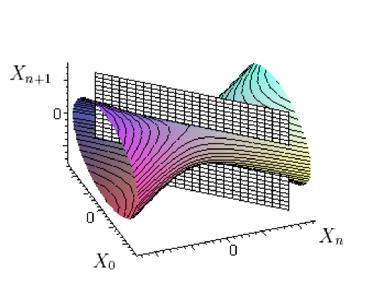
Figure 1: $AdS$ space being cut by the hyperplane $X_{0}=X_{n}$ (coordinates $X_{i}$ fixed for $i=1,..,n-1$).

III Poincaré $AdS$ boundary in global coordinates

In order to map the Poincaré $AdS$ boundary to global coordinates we first obtain relations between these two coordinates systems. From eq. (4) and eq. (10) one can find the relations

$$\sec{\rho} = \frac{1}{2R|z|}\sqrt{(z^{2}+R^{2}+{\overline{x}}^{2}-t^{2})^{2}+(2Rt)^{2}}\,,$$ (14)

$$\cos{\tau} = sgn(z)\frac{z^{2}+R^{2}+{\overline{x}}^{2}-t^{2}}{\sqrt{(z^{2}+R^{2}+{\overline{x}}^{2}-t^{2})^{2}+(2Rt)^{2}}}\,\,,\,\,\,\hbox{where}\,\,sgn(z)\equiv\frac{|z|}{z}\,,$$ (15)

$$\sin{\tau} = sgn(z)\frac{2Rt}{\sqrt{(z^{2}+R^{2}+{\overline{x}}^{2}-t^{2})^{2}+(2Rt)^{2}}}\,,$$ (16)

$$|\overline{\Omega}|\equiv\sqrt{\sum_{i=1}^{n-1}(\Omega_{i}^{2})} = \frac{2R|\overline{x}|}{\sqrt{(z^{2}+R^{2}+{\overline{x}}^{2}-t^{2})^{2}+(2Rt)^{2}-(2Rz)^{2}}}\,\,,\,\hbox{where}\,|\overline{x}|\equiv\sqrt{\overline{x}^{2}}\,\,,$$ (17)

$$\Omega_{n} = sgn(z)\frac{z^{2}-R^{2}+{\overline{x}}^{2}-t^{2}}{\sqrt{(z^{2}+R^{2}+{\overline{x}}^{2}-t^{2})^{2}+(2Rt)^{2}-(2Rz)^{2}}}\,.$$ (18)

For instance, the first relation can be obtained by adding the squares of the first and last relations in eqs. (4) and (10). These relations are valid for $z>0$ and $z<0$. For our discussion we will consider just the Poincaré chart $z>0$.

We present in table I a possible division of the Poincaré $AdS$ boundary into regions for which the coordinate transformations (14-18) lead us to well defined points in global coordinates.

Region	z	t	$|\overline{x}|$	$\rho$	$\tau$	$|\overline{\Omega}|$	$\Omega_{n}$
I	$z=0^{+}$	finite	finite	$\pi/2$	$\tau^{I}$	$|\overline{\Omega}|^{I}$	$(\Omega_{n})^{I}$
II	finite	$t\to\pm\infty$	finite	$\pi/2$	$\pm\pi$	0	-1
III	finite	finite	$|\overline{x}|\to\infty$	$\pi/2$	0	0	1
IV	finite	$t\to\pm\infty$	$|\overline{x}|\to\infty$ , $|\overline{x}|<<|t|$	$\pi/2$	$\pm\pi$	0	-1
V	finite	$t\to\pm\infty$	$|\overline{x}|\to\infty$ , $|\overline{x}|>>|t|$	$\pi/2$	0	0	1
VI	finite	$t\to\infty$	$|\overline{x}|\to\infty$ , $\overline{x}^{2}=t^{2}+\alpha|\overline{x}|$	$\pi/2$	$\tau^{VI}$	$|\overline{\Omega}|^{VI}$	$(\Omega_{n})^{VI}$
VII	finite	$t\to-\infty$	$|\overline{x}|\to\infty$ , $\overline{x}^{2}=t^{2}+\alpha|\overline{x}|$	$\pi/2$	$\tau^{VII}$	$|\overline{\Omega}|^{VII}$	$(\Omega_{n})^{VII}$
VIII	$z\to\infty$	finite	finite	$\pi/2$	0	0	1
IX	$z\to\infty$	$t\to\pm\infty$ , $z<<|t|$	finite	$\pi/2$	$\pm\pi$	0	-1
X	$z\to\infty$	$t\to\pm\infty$ , $z>>|t|$	finite	$\pi/2$	0	0	1
XI	$z\to\infty$	$t\to\infty$ , $z^{2}=t^{2}+\alpha z$	finite	$\rho^{XI}$	$\tau^{XI}$	$|\overline{\Omega}|^{XI}$	$(\Omega_{n})^{XI}$
XII	$z\to\infty$	$t\to-\infty$ , $z^{2}=t^{2}+\alpha z$	finite	$\rho^{XII}$	$\tau^{XII}$	$|\overline{\Omega}|^{XII}$	$(\Omega_{n})^{XII}$
XIII	$z\to\infty$	finite	$|\overline{x}|\to\infty$	$\pi/2$	0	0	1
XIV	$z\to\infty$	$t\to\pm\infty$ , $z^{2}+\overline{x}^{2}<<t^{2}$	$|\overline{x}|\to\infty$	$\pi/2$	$\pm\pi$	0	-1
XV	$z\rightarrow\infty$	$t\to\pm\infty$ , $z^{2}+\overline{x}^{2}>>t^{2}$	$|\overline{x}|\to\infty$	$\pi/2$	0	0	1
XVI	$z\to\infty$	$t\to\infty$ ,	$|\overline{x}|\to\infty$ , $\overline{x}^{2}=\beta^{2}z^{2}$	$\rho^{XVI}$	$\tau^{XVI}$	$|\overline{\Omega}|^{XVI}$	$(\Omega_{n})^{XVI}$
		$z^{2}+\overline{x}^{2}=t^{2}+\alpha z$
XVII	$z\to\infty$	$t\to-\infty$ ,	$|\overline{x}|\to\infty$ , $\overline{x}^{2}=\beta^{2}z^{2}$	$\rho^{XVII}$	$\tau^{XVII}$	$|\overline{\Omega}|^{XVII}$	$(\Omega_{n})^{XVII}$
		$z^{2}+\overline{x}^{2}=t^{2}+\alpha z$

Table 1: Poincaré $AdS$ boundary divided into different regions corresponding to well defined points in global coordinates. The parameters $\alpha$ and $\beta$ are finite with $\beta\neq 0$.

In this table we use the following definitions :

• In region I , we have that $\rho^{I}=\pi/2$. The coordinates $\tau^{I},|\overline{\Omega}|^{I}$ and $(\Omega_{n})^{I}$ are given by the relations

  $$\cos{\tau^{I}} = \frac{R^{2}+{\overline{x}}^{2}-t^{2}}{\sqrt{(R^{2}+{\overline{x}}^{2}-t^{2})^{2}+(2Rt)^{2}}}\,,$$

  $$\sin{\tau^{I}} = \frac{2Rt}{\sqrt{(R^{2}+{\overline{x}}^{2}-t^{2})^{2}+(2Rt)^{2}}}\,,$$

  $$|\overline{\Omega}|^{I} = \frac{2R|\overline{x}|}{\sqrt{(R^{2}+{\overline{x}}^{2}-t^{2})^{2}+(2Rt)^{2}}}\,,$$

  $$(\Omega_{n})^{I} = \frac{-R^{2}+{\overline{x}}^{2}-t^{2}}{\sqrt{(R^{2}+{\overline{x}}^{2}-t^{2})^{2}+(2Rt)^{2}}}\,.$$ (19)

  This region corresponds to the hyperplane $z=0$ . It is interpreted as the Minkowski space-time and is part of the global $AdS$ boundary .

• Regions VI and VII satisfy the condition $\cos{\tau}=\Omega_{n}$ for $z$ finite (this condition was discussed in the previous section). These regions belong to the global $AdS$ boundary because $\rho=\pi/2$.

  The points of region VI are defined by the following relations :

  $$\cos{\tau^{VI}} = (\Omega_{n})^{VI}=\left\{\begin{array}[]{ll}\pm\frac{1}{\sqrt{1+(\frac{2R}{\alpha})^{2}}}&,\mbox{for $sgn(\alpha)=\pm 1$ }\\ 0&,\mbox{for $\alpha=0$}\end{array}\right.\,,\,\,0\leq\tau^{VI}\leq\pi\,,\,\,$$ (22)

  $$|\overline{\Omega}|^{VI} = \frac{1}{\sqrt{1+(\frac{\alpha}{2R})^{2}}}\,\,\,.$$ (23)

  Region VII has the same points as in VI with the difference that $-\pi\leq\tau^{VII}\leq 0$   .

• Regions XI, XII, XVI and XVII correspond to special cases of the limit $z\to\infty$ , $t\to\pm\infty$. These regions belong to the cutting hyperplane and the hyperboloid. The points of region XI are defined by

  $$\sec{\rho^{XI}} = \sqrt{1+(\frac{\alpha}{2R})^{2}}\,\,,\,\,(0<\rho<\pi/2),$$

  $$\cos{\tau^{XI}} = \sin{\rho^{XI}}(\Omega_{n})^{XI}\,\,,\,\,\hbox{with}\,\,0\leq\tau^{XI}\leq\pi\,,$$

  $$|\overline{\Omega}|^{XI} = \left\{\begin{array}[]{ll}0&,\mbox{ if $\alpha\neq 0$}\\ \frac{2R|\overline{x}|}{R^{2}+\overline{x}^{2}}&,\,\mbox{if $\alpha=0$}\end{array}\right.\,,$$ (26)

  $$(\Omega_{n})^{XI} = \left\{\begin{array}[]{ll}1&,\,\mbox{ if $\alpha\neq 0$}\\ \frac{-R^{2}+\overline{x}^{2}}{R^{2}+\overline{x}^{2}},&\mbox{if $\alpha=0$}\end{array}\right.\,.$$ (29)

  For region XII we have the same points of the region XI with the difference that now $-\pi\leq\tau^{XII}\leq 0$ .

  For region XVI we have that

  $$\sec{\rho^{XVI}} = \sqrt{1+(\frac{\alpha}{2R})^{2}+\beta^{2}}\,\,,$$

  $$\cos{\tau^{XVI}} = \sin{\rho^{XVI}}(\Omega_{n})^{XVI}\,,\,\hbox{with}\,\,0\leq\tau^{XVI}\leq\pi\,,$$

  $$(\Omega_{n})^{XVI} = \left\{\begin{array}[]{ll}\pm\frac{1}{\sqrt{1+(\frac{2R\beta}{\alpha})^{2}}},&\mbox{for $sgn(\alpha)=\pm 1$ }\\ 0&,\,\,\mbox{for $\alpha=0$}\end{array}\right.\,,$$ (32)

  $$|\overline{\Omega}|^{XVI} = \frac{1}{\sqrt{1+(\frac{\alpha}{2R\beta})^{2}}}\,.$$ (33)

  For region XVII we have the same points of region XVI with the difference that now $-\pi\leq\tau^{XVII}\leq 0$ .

• Regions II, IV, IX, and XIV correspond to the unique point $\rho=\pi/2,\tau=0,\break|\overline{\Omega}|=0,\Omega_{n}=1$. This corresponds to point $A$ in figure 2(b).

• Similarly, regions III, V, VIII, X, XIII and XV correspond to the unique point $\rho=\pi/2,\tau=\pm\pi,|\overline{x}|=0,\Omega_{n}=-1$. This corresponds to point $B$ in figure 2(b).

  These two special points belong to the boundary of the hyperboloid and the cutting hyperplane $X_{0}=X_{n}$ because $z\to\infty$.

All these results are shown in Figure 2, where we draw the Penrose diagram for $AdS$ space. We can see there that the Poincaré $AdS$ boundary contains points of the global $AdS$ boundary $\rho=\pi/2$ and points of the global $AdS$ bulk. So we conclude that the Poincaré $AdS$ boundary is not the same as the global $AdS$ boundary.

It is important to observe that regions XI,XII XVI and XVII, which correspond to points in the bulk of the global AdS, have a singular metric in the Poincaré coordinate system. These regions can be described in a non singular way returning to global coordinates.

It is also very interesting to note that there are some regions of the Poincaré $AdS$ boundary that corresponds to single points in global coordinates, so there must be some kind of identifications between these regions. Note that these regions may have different embedding space coordinates. For example, from eq. (10) we find that region II corresponds to finite $X_{i}$ while region IX corresponds to $X_{i}\,=\,0\,$. This happens because the relation (4) between global coordinates and embedding coordinates is one to one just for points of the hyperboloid but not for points of the boundary $\rho=\pi/2$. This means that different points of the infinity of the hyperboloid are mapped to single points in global coordinates. This situation is similar to what happens when a 2D Minkowski space time $(x,t)$ is compactified to the interior of a rectangle and the spatial infinity $x\to\infty$ is mapped to just one point of the rectangle (the same point for all finite values of $t$).

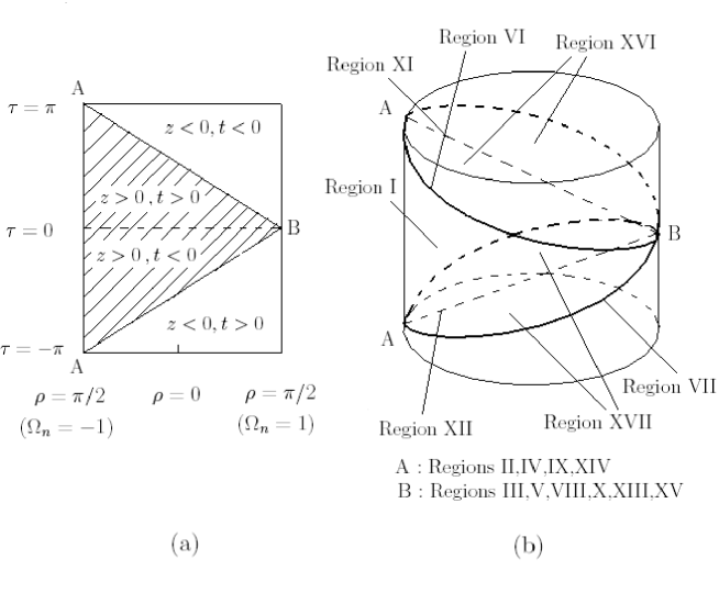
Figure 2: (a) Penrose diagram for $AdS$ space, the Poincaré $AdS$ space corresponds to the dashed region. (b) Poincaré $AdS$ boundary regions described in the Penrose diagram in 3D.

IV The Euclidean $AdS$ space

The isometry group of $AdS_{n+1}$ space in the Lorentzian case is $SO(2,n)$ while in the Euclidean case it is $SO(1,n+1)$. In the AdS/CFT correspondence the conformal group of the boundary theory is isomorphic to the isometry group of the bulk gravity theory, so the conformal theories are not the same. We will see that the boundaries of Euclidean and Lorentzian AdS spaces, where the conformal theories are defined are different.

When calculating conformal correlation functions one finds different results taking Lorentzian or Euclidean signatures for the AdS metric. As discussed in Balasubramanian:1998de , in the Lorentzian case there are normalizable modes in the solutions of the bulk fields. These normalizable modes are related to states in the boundary CFT. So in the Lorentzian case, using the AdS/CFT correspondence one can calculate operator expectation values in excited states of the conformal theory.

In the Euclidean case there are no normalizable modes in the solutions of the field equations. The solutions are uniquely determined by the boundary values of the fields. In this case one calculates operator expectation values in the vacuum.

We will now describe the Euclidean AdS boundary in Poincaré coordinates. The geometry of this boundary is more simple than the Lorentzian case. We can go to Euclidean signature performing a rotation in the time coordinate

$$t\to it\,,$$ (34)

This rotation Aharony induces a rotation on the embedding (time-like) coordinate $X_{n+1}$ :

$$X_{n+1}\to iX_{n+1}\,.$$ (35)

So we have that relations (10) become

$$X_{0} = \frac{1}{2z}(z^{2}+R^{2}+{\overline{x}}^{2}+t^{2})\,,$$

$$X_{i} = \frac{Rx^{i}}{z}\,,\hskip 28.45274pti=1,..,n-1\,,$$

$$X_{n} = -\frac{1}{2z}(z^{2}-R^{2}+{\overline{x}}^{2}+t^{2})\,,$$

$$X_{n+1} = \frac{Rt}{z}\,.$$ (36)

We also see from (35) and (2) that the equation of the hyperboloid is now

$$X_{0}^{2}-X_{n+1}^{2}-\sum_{i=1}^{n}X_{i}^{2}=R^{2}\,,$$ (37)

(note the different sign). This equation defines the so-called Euclidean $AdS$ space, this equation can be solved by the following relations :

$$X_{0} = R\sec{\rho}\sec{\tau}\,,$$

$$X_{i} = R\tan{\rho}\Omega_{i}\,,\hskip 28.45274pti=1,..,n\,,$$

$$X_{n+1} = R\sec{\rho}\tan{\tau}\,$$ (38)

where $\sum_{i=1}^{n}{{\Omega_{i}}^{2}}=1$. The relations (38) define a new chart that we will call semi-global chart because it can describe only one half of the hyperboloid. For example, the first half of the hyperboloid ($z>0$) corresponding to the region $X_{0}\geq R$ can be obtained by taking in (38) the range $-\frac{\pi}{2}<\tau<\frac{\pi}{2}$ . The other half ($z<0$) corresponding to the region $X_{0}\leq-R$ can be also obtained by working in the range $\frac{\pi}{2}<\tau<\frac{3\pi}{2}$.

It is interesting to note that the cutting hyperplane $X_{0}=X_{n}$, described in section II, does not contain points of the entire Euclidean $AdS$ space because this condition is not compatible with (37).

We can find a map of the Euclidean $AdS$ boundary to this semi-global chart. For this purpose, we obtain relations between Euclidean Poincaré coordinates and semi-global coordinates in the same way as in section III:

$$\sec{\rho} = \frac{1}{2R|z|}\sqrt{(z^{2}+R^{2}+{\overline{x}}^{2}+t^{2})^{2}-(2Rt)^{2}}\,,$$

$$\sec{\tau} = sgn(z)\frac{z^{2}+R^{2}+{\overline{x}}^{2}+t^{2}}{\sqrt{(z^{2}+R^{2}+{\overline{x}}^{2}+t^{2})^{2}-(2Rt)^{2}}}\,,$$

$$\tan{\tau} = sgn(z)\frac{2Rt}{\sqrt{(z^{2}+R^{2}+{\overline{x}}^{2}+t^{2})^{2}-(2Rt)^{2}}}\,,$$

$$|\overline{\Omega}| = \frac{2R|\overline{x}|}{\sqrt{(z^{2}+R^{2}+{\overline{x}}^{2}+t^{2})^{2}-(2Rt)^{2}-(2Rz)^{2}}}\,,\,\,\hbox{where}\,|\overline{x}|\equiv\sqrt{\overline{x}^{2}}\,\,,$$

$$\Omega_{n} = sgn(z)\frac{z^{2}-R^{2}+{\overline{x}}^{2}+t^{2}}{\sqrt{(z^{2}+R^{2}+{\overline{x}}^{2}+t^{2})^{2}-(2Rt)^{2}-(2Rz)^{2}}}\,.$$

Region I, defined in the last section, corresponds in Euclidean Poincaré coordinates to an Euclidean space and can be mapped to the semi-global chart. The semi-global coordinates corresponding to this region are given by

$$\rho^{I} = \pi/2\,,$$

$$\sec{\tau^{I}} = \frac{R^{2}+{\overline{x}}^{2}+t^{2}}{\sqrt{(R^{2}+{\overline{x}}^{2}+t^{2})^{2}-(2Rt)^{2}}}\,,$$

$$\tan{\tau^{I}} = \frac{2Rt}{\sqrt{(z^{2}+R^{2}+{\overline{x}}^{2}+t^{2})^{2}-(2Rt)^{2}}}\,,$$

$$|\overline{\Omega}|^{I} = \frac{2R|\overline{x}|}{\sqrt{(R^{2}+{\overline{x}}^{2}+t^{2})^{2}-(2Rt)^{2}}}\,,$$

$$(\Omega_{n})^{I} = \frac{-R^{2}+{\overline{x}}^{2}+t^{2}}{\sqrt{(R^{2}+{\overline{x}}^{2}+t^{2})^{2}-(2Rt)^{2}}}\,.$$ (40)

The other regions correspond in semi-global coordinates to the unique point $\rho=\pi/2,\,\break\tau=0\,\,|\overline{\Omega}|=0\,,\,\Omega_{n}=1$. This point does not belong to region I, it belongs to the boundary of the hyperboloid and to the cutting hyperplane $X_{0}=X_{n}$. We conclude that the Euclidean AdS boundary in Poincaré coordinates is the Euclidean space region $\rm l\!R\,^{n}\,$ at $z=0$ plus one point at infinity. This is different from the Lorentzian case where the boundary is $\rm l\!R\,^{1,n-1}\,$ plus the other regions described in section III.

This way we found an equivalence between the Euclidean Poincaré chart and the semi-global chart, because they describe in fact the same space with the same boundary.

V Conclusions

We found a detailed map of the boundary of Poincaré $AdS$ space to the global coordinate chart. We studied also the origin of Poincaré $AdS$ space as a subspace of the global $AdS$. From the map, described in section III, we conclude that if a Poincaré $AdS$ space corresponds in fact to a subspace of the global $AdS$ we have to impose the identification of some regions of its boundary. In the Euclidean case, we proposed a semi-global chart that describes the same space as the Euclidean Poincaré chart. The identification of boundary regions of the Euclidean Poincaré chart is trivial.

The AdS/CFT correspondence is usually interpreted as a realization of the holographic principle. This interpretation depends on the assumption that the region $z=0$ plus some isolated points at infinity is the boundary of the Poincaré AdS space. Since the isolated points do not carry degrees of freedom, the correspondence between a field theory in the Poincaré AdS and a theory on $z=0$ is taken as a bulk/boundary correspondence. Here we conclude that this interpretation is not correct because the Minkowski space, even after compactification, is not the complete boundary of the Poincaré AdS space. This boundary actually includes other regions of the global AdS space (see for instance regions XVI, XVII). The bulk/boundary interpretation is correct for the Euclidean case, where indeed the boundary is the region $z=0$ plus a point at infinity.

- (1) J. M. Maldacena, Adv. Theor. Math. Phys. 2, 231 (1998).
- (2) J. L. Petersen, Int. J. Mod. Phys. A 14, 3597 (1999).
- (3) O. Aharony, S.S. Gubser, J.M. Maldacena, H.Ouguri,Y.Oz., Phys. Report 323, 183 (2000).
- (4) E. D’Hoker and D. Z. Freedman, “Supersymmetric gauge theories and the AdS/CFT correspondence,” arXiv:hep-th/0201253.
- (5) G. Horowitz and A. Strominger, Nucl. Phys. B 360, 197 (1991).
- (6) S. J. Avis, C. J. Isham and D. Storey, Phys. Rev. D 18, 3565 (1978).
- (7) P. Breitenlohner and D. Z. Freedman, Phys. Lett. B 115, 197 (1982).
- (8) S. S. Gubser, I.R. Klebanov, A. M. Polyakov, Phys. Lett. B 428, 105 (1998).
- (9) E. Witten, Adv. Theor. Math. Phys. 2, 253 (1998).
- (10) G. ’t Hooft, ”Dimensional reduction in quantum gravity” in Salam Festschrifft, eds. A. Aly, J. Ellis and S. Randjbar-Daemi, World Scientific, Singapore, 1993, gr-qc/9310026.
- (11) L. Susskind, J. Math. Phys. 36, 6377 (1995).
- (12) E.Witten, S.T.Yau, Adv. Theor. Math. Phys. 3, 1635 (1999).
- (13) H. Boschi-Filho and N. R. F. Braga, Phys. Rev. D 66, 025005 (2002).
- (14) V. Balasubramanian, P. Kraus and A. E. Lawrence, Phys. Rev. D 59, 046003 (1999).
- (15) H. Boschi-Filho and N. R. F. Braga, Phys. Lett. B 505, 263 (2001).
- (16) R. Emparan, C. V. Johnson and R. C. Myers, Phys. Rev. D 60, 104001 (1999).
- (17) V. Balasubramanian and P. Kraus, Commun. Math. Phys. 208, 413 (1999).
- (18) D. Astefanesei, R. B. Mann and E. Radu, JHEP 0501, 049 (2005).
- (19) E. Witten, Adv. Theor. Math. Phys. 2, 505 (1998).
- (20) V. Balasubramanian, P. Kraus, A. E. Lawrence and S. P. Trivedi, Phys. Rev. D 59, 104021 (1999).