December 2005 KUNS-2003 hep-th/0512176

Nonperturbative Effect
in $c=1$ Noncritical String Theory
and Penner Model

Yoshinori Matsuo

Department of Physics, Kyoto University, Kyoto 606-8502, Japan

We derive the effect of instantons in the Penner model. It is known that the free energies of the Penner model and the $c=1$ noncritical string at self-dual radius agree in a suitable double scaling limit. On the other hand, the instanton in the matrix model describes a nonperturbative effect in the noncritical string theory. We study the correspondence between the instantons in the Penner model and the nonperturbative effect in $c=1$ noncritical string at self-dual radius.

1 Introduction

After the discovery of the D-brane, which is the typical nonperturbative effect in the string theory, the study of the nonperturbative effect is of great interest. We can analyze the noncritical string theory, which is a simplified model of the string theory, nonperturbatively via the matrix model (for reviews, see [1, 2, 3]). The nonperturbative effect in noncritical string theory can be derived via the string equation. On the other hand, this effect appears as the instanton when we directly analyze the matrix model. The string equation cannot describe the whole of the nonperturbative effect. There is an ambiguity that corresponds to the initial condition of the string equation. Studying the matrix model directly, we can fix it [4].

This analysis is generalized to various models [5, 6, 7]. One of the most interesting models is the $c=1$ noncritical string theory because it describes the dynamics of strings in two dimensional space-time. In this paper, we consider the Penner model, which corresponds to the $c=1$ noncritical string theory with one direction of the space-time compactified on the circle with self-dual radius [8].

The Penner model is defined as a kind of the hermitian one-matrix model. Therefore, we can extend the analysis for the $c=0$ matrix model to our case with a small modification. And, it is easy to see that the relation between the nonperturbative effect for the $c=0$ matrix model and that in the Penner model. In this paper, we generalize the analysis of the instanton in the $c=0$ matrix model to the case of the Penner model. And we show that some of the nonperturbative effect in the $c=1$ noncritical string theory can be understood as the effects of instantons in the Penner model.

This paper is organized as follows. First, in section 2, we consider the instanton in the $c=0$ matrix model. We also give the interpretation which makes it possible to extend the analysis to the case of the Penner model. In section 3, we summarize some of the known facts related to the correspondence between the Penner model and the $c=1$ noncritical string theory. In section 4, we make the redefinition of the Penner model to introduce the instantons, and calculate the contribution from the instantons to the free energy. In section 5 is devoted for the conclusions and discussions. In appendices, we show the details of calculations and the behaviors of orthogonal polynomials in large $N$ limit.

2 The instantons in $c=0$ noncritical string theory

Before studying the effect of instantons for the $c=1$ noncritical string theory, in this section, we review the results obtained in the case of the $c=0$ noncritical string theory [4]. We focus on the contribution of instantons to the free energy. In order to extend the instanton calculation to the $c=1$ case, we also give the precise definition of instanton.

The $c=0$ noncritical string theory can be described by the hermitian one-matrix model. Its partition function is given by

$$Z=\int\mathrm{d}\Phi\,\mathrm{e}^{-N\mathop{\mathrm{tr}}V(\Phi)},$$ (2.1)

where $\Phi$ is an $N\times N$ hermitian matrix. By diagonalizing the matrix $\Phi$, this theory can be described by eigenvalues of the matrix $\Phi$, and the partition function can be expressed as

$$Z=\int\prod_{i}\mathrm{d}\lambda_{i}\Delta^{2}(\lambda)\,\mathrm{e}^{-N\sum_{i}V(\lambda_{i})}.$$ (2.2)

Vandermonde determinant is defined as $\Delta(\lambda)=\prod_{i<j}(\lambda_{i}-\lambda_{j})$. Here, we concentrate on the $N$-th eigenvalue $\lambda_{N}$ and represent it $x$. Integrating out the other $N-1$ eigenvalues, we obtain the effective potential $V_{\text{eff}}(x)$ of the $N$-th eigenvalue $x=\lambda_{N}$. The partition function can be expressed using the effective potential as

$$Z=\int\mathrm{d}x\,\mathrm{e}^{-NV_{\text{eff}}(x)}=Z_{N-1}\int\mathrm{d}x\left\langle\det(x-\Phi)^{2}\right\rangle_{N-1}\mathrm{e}^{-NV(x)},$$ (2.3)

where the subscript “$N-1$” indicate that the matrix $\Phi$ is replaced by an $(N-1)\times(N-1)$ matrix. In the large $N$ limit, the system of an $N\times N$ matrix gives the same results as one of an $(N-1)\times(N-1)$ matrix. Hence, we can replace it by the expectation value of the standard $N\times N$ matrix

$$\left\langle\mathcal{O}\right\rangle=\frac{1}{Z}\int\mathrm{d}\Phi\ \mathcal{O}\,\mathrm{e}^{-N\mathop{\mathrm{tr}}V(\Phi)}.$$ (2.4)

In the large $N$ limit, the effective potential $V_{\text{eff}}(x)$ can be expressed using the resolvent $R(x)=\frac{1}{N}\left\langle\mathop{\mathrm{tr}}\frac{1}{x-\Phi}\right\rangle$ as

$$V_{\text{eff}}(x) =V(x)-2\mathop{\mathrm{Re}}\int^{x}\mathrm{d}x^{\prime}\,R(x^{\prime})$$

$$=\mathop{\mathrm{Re}}\int^{x}\mathrm{d}x^{\prime}\sqrt{V^{\prime 2}(x^{\prime})+4f(x^{\prime})},$$ (2.5)

at the leading order of the $\frac{1}{N}$ expansion. Now we consider the model corresponding to the $c=0$ noncritical string theory. Taking the double scaling limit, we obtain

$$V_{\text{eff}}(x)=\text{const.}\times\mathop{\mathrm{Re}}\int^{x}\mathrm{d}x^{\prime}\left(x^{\prime}-\frac{1}{2}\sqrt{t}\right)\sqrt{x^{\prime}+\sqrt{t}}.$$ (2.6)

The first derivative of the effective potential vanishes in two regions. One is the region where the resolvent has the cut. The effective potential takes a constant value in this region, and it is local minimum. The other is the point of $x=\frac{1}{2}\sqrt{t}$ where the effective potential has local maximum. The region of the cut gives the dominant contribution, which corresponds to the perturbative expansion. We call this region as “dominant saddle point.” And the point of the local maximum of the effective potential gives sub-dominant contribution, which corresponds to the nonperturbative effect. We call this point as “sub-dominant saddle point,” and this sub-dominant contribution, or the configuration in which one or more eigenvalues are at this “sub-dominant saddle point,” as “instanton.”

Up to this point, we have restricted ourselves to the $N$-th eigenvalue. However, there are $N$ eigenvalues and all of them can be possibly at the “sub-dominant saddle point.” Including these, we obtain

$$Z =Z^{(\text{0-inst})}+Z^{(\text{1-inst})}+Z^{(\text{2-inst})}+\cdots,$$ (2.7a)

$$Z^{(\text{0-inst})} =\int_{\text{inside the cut}}\prod_{i}\mathrm{d}\lambda_{i}\,\Delta^{2}(\lambda)\,\mathrm{e}^{-N\mathop{\overset{}{\underset{i}{\textstyle\sum}}}V(\lambda_{i})}$$

$$=Z^{(\text{0-inst})}_{N-1}\int_{\text{inside the cut}}\mathrm{d}x\left\langle\det(x-\Phi)^{2}\right\rangle^{(\text{0-inst})}\mathrm{e}^{-NV(x)},$$ (2.7b)

$$Z^{(\text{1-inst})} =NZ^{(\text{0-inst})}_{N-1}\int_{\text{outside the cut}}\mathrm{d}x\left\langle\det(x-\Phi)^{2}\right\rangle^{(\text{0-inst})}\mathrm{e}^{-NV(x)}.$$ (2.7c)

We have divided the integration region, namely, inside the cut and outside the cut. The “dominant saddle point” is identical to the region inside the cut, and the “sub-dominant saddle point” is included in the region outside the cut. The superscript “0-inst” indicates that all eigenvalues are inside the cut and “$n$-inst” indicates that $n$ eigenvalues are outside the cut.

By neglecting the interaction between the eigenvalues, the free energy becomes

$$e^{F}=Z =Z^{(\text{0-inst})}\left(1+\frac{Z^{(\text{1-inst})}}{Z^{(\text{0-inst})}}+\cdots\right)=\mathrm{e}^{F^{(\text{0-inst})}+\delta F},$$ (2.8a)

$$F^{(\text{0-inst})}=-\frac{4}{15}t^{\frac{5}{2}}$$ (2.8b)

$$\delta F=\frac{Z^{(\text{1-inst})}}{Z^{(\text{0-inst})}}=\frac{i}{16\cdot 3^{\frac{3}{4}}\sqrt{\pi}t^{\frac{5}{8}}}\exp\left[-\frac{8\sqrt{3}}{5}t^{\frac{5}{4}}\right].$$ (2.8c)

Now, we consider why the nonperturbative correction of the free energy becomes imaginary. The partition function of the matrix model is defined as an integration of a real function. By this definition, the free energy of this model should be real. To obtain the imaginary number, some change of the definition is needed. The imaginary part of the free energy reflects the instability of the model. In the $c=0$ matrix model, all the eigenvalues distribute around one minimum of the potential. This minimum corresponds to the “dominant saddle point.” However, the potential of the $c=0$ matrix model has some local minima other than this, or it is unbounded from below. To prevent the eigenvalues from distributing around these unwanted minima, or the unbounded region, we should deform the contour of the integration. We integrate the effective potential over $x$ along the real axis around the minimum corresponding to the “dominant saddle point,” and the contour turns at right angle after reaching the “sub-dominant saddle point.”(Fig. 1) Then, we have the integration orthogonal to the real axis at the “sub-dominant saddle.” It gives an imaginary number. This modification of the curve of the integration is needed for all eigenvalues, and chosen not to include the unwanted vacua. Because we can define the partition function by the integration of the analytic function, the partition function depends only on the beginning and the end of the contour.

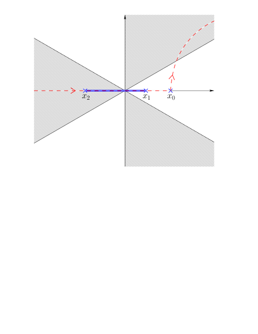
Figure 1: The cut of the resolvent (the bold line) and the contour of the integration (the dashed line) corresponding to the $c=0$ noncritical string theory. Here, we consider a cubic potential for instance. We should put the beginning and the end of the contour at $|z|\to\infty$ in the shaded region.

For example, we take a cubic potential $V(x)=\frac{1}{2}x^{2}-\frac{g}{3}x^{3}$ In this case, the potential is unbounded from below. Then, we should define the integration so as to avoid this divergence. On the other hand, the partition function is defined as

$$Z=\int\prod_{i}\mathrm{d}\lambda_{i}\Delta^{2}(\lambda)\mathrm{e}^{-N\sum_{i}V(\lambda_{i})}.$$ (2.9)

If we define the contour of the integration to be along the real axis, the integrand is diverges at $x\to\infty$. Generally, we assume that the contribution from boundary terms of integration vanishes in the $c=0$ matrix model. It can be done by taking the beginning and the end of the contour to be $|\lambda|\to\infty$ in the shaded region in Fig. 1 — $-\frac{\pi}{2}<\arg\lambda<-\frac{1}{6}\pi$, $\frac{1}{6}\pi<\arg\lambda<\frac{\pi}{2}$ or $\frac{5}{6}\pi<\arg\lambda<\frac{7}{6}\pi$. Now, we put the beginning of the contour in the region $|\lambda|\to\infty$ and $\frac{5}{6}\pi<\arg\lambda<\frac{7}{6}\pi$, and the end of the contour in $|\lambda|\to\infty$ and $\frac{1}{6}\pi<\arg\lambda<\frac{\pi}{2}$. Then, we obtain the wanted integration: the dominant contribution comes from the cut. It correspond to the $c=0$ noncritical string theory. If we put the beginning and the end of the contour in the region $-\pi<\arg\lambda<-\frac{1}{6}\pi$ and $\frac{1}{6}\pi<\arg\lambda<\pi$, integration does not include the contribution from the cut. This definition of the integration does not correspond to the $c=0$ noncritical string theory. Thus, the choice of the beginning and the end of the contour determines which vacua are included in the theory.

We take the contour corresponding to the $c=0$ noncritical string theory. The contributions from the perturbative expansion are divergent series, and the instantons give corrections to this series. Therefore, it isn’t well-defined. But If we restrict ourselves on the imaginary part of the free energy, the situation becomes different. The contributions of a perturbative expansion are real because they come from the integration inside the cut. Hence, the dominant contribution of the imaginary part comes from the instanton. Therefore, the imaginary part of the nonperturbative effect is well-defined. In this way, we have obtained the imaginary part of the nonperturbative effect.

3 The Penner model and the $c=1$ noncritical string

In this section, we study the Penner model. The Penner model is defined as a hermitian one-matrix model with a logarithmic potential. It is noted that in the suitable double scaling limit, the free energy of the Penner model is identical to that of the $c=1$ noncritical string theory with the target space compactified on the circle of self-dual radius $R=1$ [8, 9]. Here, we review the relation between the Penner model and $c=1$, $R=1$ noncritical string theory.

The Penner model is defined as a hermitian one-matrix model with the following potential:

$$V(x)=\frac{1}{g}\left(x-\log x\right).$$ (3.1)

We can derive the free energy via the method of orthogonal polynomials. This method makes use of an infinite set of polynomials obeying the orthogonality condition:

$$(P_{n}(x),P_{m}(x))=\int\mathrm{d}x\,P_{n}(x)P_{m}(x)\,\mathrm{e}^{-NV(x)}=h_{n}\delta_{nm}.$$ (3.2)

The normalization of orthogonal polynomials is given by having leading term $P_{n}(x)=x^{n}+\cdots$. The partition function of the hermitian one-matrix model is given by

$$Z=N!\prod_{n=0}^{N-1}h_{n}.$$ (3.3)

So, we should calculate $h_{n}$. Orthogonal polynomials satisfy the following two recursion relations,

$$xP_{n}(x) =X_{nm}P_{m}(x)=P_{n+1}(x)+s_{n}P_{n}(x)+r_{n}P_{n-1}(x),$$ (3.4a)

$$P_{n}^{\prime}(x) =\mathcal{P}_{nm}P_{m}(x)=\left[NV^{\prime}(X)\right]_{nm}P_{m}(x).$$ (3.4b)

Using these relations, we can easily see that $r_{n}=\frac{h_{n}}{h_{n-1}}$. For the case of the Penner model (3.1), these recursion relations are exactly soluble. Solutions of these relations are

$$r_{n} =g\xi(g\xi+1)$$ (3.5a)

$$s_{n} =1+2g\xi+\frac{g}{N}.$$ (3.5b)

The partition function of the model is given by $Z=N!\prod_{n}h_{n}$, and the free energy is

$$F=N\sum_{n}\left(1-\frac{n}{N}\right)\log r_{n}.$$ (3.6)

To obtain the free energy identical to the $c=1$ and $R=1$ noncritical string theory, we take the following double scaling limit

$$N(1+g) =t, N \to\infty,$$ (3.7)

and replace the summation over $n$ by integration with respect to $\xi=\frac{n}{N}$ via Euler-Maclaurin summation formula. Then, we obtain

$$F=\frac{1}{2}t^{2}\log t-\frac{1}{12}\log t+\sum_{h=1}^{\infty}\frac{B_{2h}}{2h(2h-2)}t^{2-2h},$$ (3.8)

up to regular terms. Taking $t=i\mu$, we obtain

$$F=-\frac{1}{2}\mu^{2}\log\mu-\frac{1}{12}\log\mu+\sum_{h=1}^{\infty}\frac{\left\lvert B_{2h}\right\rvert}{2h(2h-2)}\mu^{2-2h}.$$ (3.9)

This expression is identical to the free energy of the $c=1$ noncritical string theory compactified on the circle with self-dual radius.

To see the precise behavior of the Penner model, we consider the resolvent and the concrete expressions of orthogonal polynomials. First, we consider the resolvent. In the large $N$ limit, we can derive the resolvent $R(x)=\frac{1}{N}\left\langle\mathop{\mathrm{tr}}\frac{1}{x-\Phi}\right\rangle$ from the loop equation, and we obtain

$$R(x) =\frac{1}{N}\left\langle\mathop{\mathrm{tr}}\frac{1}{x-\Phi}\right\rangle$$

$$=\frac{1}{2gx}\left(x-1\pm\sqrt{x^{2}-2(1+2g)x+1}\right).$$ (3.10)

Here, the sign of “$\pm$” is depends on the location of the cut. The position of the cut is identical to the support of the eigenvalue density. It is determined by the following function $G(x)$.

$$G(x)=\int_{x_{1}}^{x}\mathrm{d}x^{\prime}\left(V^{\prime}(x^{\prime})-2R(x^{\prime})\right)$$ (3.11)

The support of the eigenvalue density is an arc connecting two branch points of the resolvent satisfying the following two conditions: the real part of $G(x)$ vanishes along this support and the real part of $G(x)$ is negative around this support [9, 10]. Here, we put $x_{1}$ on one of branch points of the resolvent.

The Penner model is defined with positive coupling constant $g>0$ in (3.1). We also restrict the integration to positive eigenvalues, from $\lambda=0$ to $\lambda\to+\infty$. Therefore there are contributions the boundaries at $\lambda=0$ and $\lambda\to+\infty$. These contributions vanish for $g>0$. However, to obtain the model corresponding to the $c=1$ noncritical string theory, $g$ should be negative. We calculate the free energy, or some expectation value, with positive $g$, and at the end, analytically continue the result to negative $g$.

In this process, we use the fact that boundary terms of the integration vanish for positive $g$. However, under the analytic continuation to negative $g$, it is merely an assumption that boundary terms can be dropped. In fact, if we use the contour of the integration which is used in the case of positive $g$, boundary terms do not vanish for negative $g$. Therefore we should deform the contour to drop boundary terms.

As is the case with the model corresponding to the $c=0$ noncritical string theory, we can determine the contour of the integration by specifying the position of its both ends. For the Penner model, boundary terms vanish when we put the boundary in the region where $|\lambda|\to\infty$ with real part of eigenvalues negative. Because the beginning and the end of the contour are located at the same point, the contour should go around the singularity of the logarithmic potential of the Penner model to obtain a nontrivial result. Then, the contour of the integration becomes as indicated in Fig. 2. The position of the cut changes depends on the choice of the contour. For positive $g$, the cut is located on the positive real axis and the contour can be taken to be along the cut. For negative $g$, both ends of the cut have the imaginary part, and the cut intersect the real axis on its positive part.(Fig. 2) The result of the integration doesn’t change under the deformation of the contour which doesn’t move the both ends and doesn’t cross singularity. And the position of the cut has been determined when we have specified the position of the both ends of the contour. Then, we can take the contour to be along the cut.

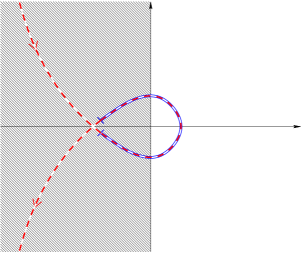
Figure 2: The contour of the integration (the dashed line) and the cut of the resolvent (the bold line) for the Penner model with negative $g$. We should put both ends of the contour at $|\lambda|\to\infty$ in the shaded region. The support of the eigenvalue distribution is along the contour, and no longer on the real axis.

Next, we consider the concrete expression of orthogonal polynomials. We show only the result here, and the detailed calculations are given in Appendix A. In large $N$ limit, orthogonal polynomials can be written as

$$\psi_{n}(x) =\frac{1}{\sqrt{h_{n}}}P_{n}(x)\,\mathrm{e}^{-\frac{1}{2}NV(x)}$$

$$=\left(\frac{(x-(1+2g\xi)+\sqrt{x^{2}-2(1+2g\xi)x+1})^{2}}{4g\xi(g\xi+1)(x^{2}-2(1+2g\xi)+1)}\right)^{\frac{1}{4}}\exp\left[-\frac{N\xi}{2}G_{\xi}(x)\right],$$ (3.12)

where, $G_{\xi}(x)$ is $G(x)$ with $g$ replaced by $g\xi$.

4 Instantons in the Penner model

In this section, we consider the effect of the instanton in the Penner model. In the case of the $c=0$ matrix model, the model is a hermitian one-matrix model, and its dynamics can be reduced to that of the eigenvalues. The instanton is defined as the configuration in which one of the eigenvalues is located at the local maximum of the effective potential. The Penner model is also a hermitian one-matrix model. We can use the same definition of the instanton as that for the case of the $c=0$ theory.

The effective potential of an eigenvalue of a hermitian one matrix model is defined as

$$Z=\int\mathrm{d}x\,\mathrm{e}^{-NV_{\text{eff}}(x)}=Z_{N-1}\int\mathrm{d}x\left\langle\det(x-\Phi)^{2}\right\rangle_{N-1}\mathrm{e}^{-NV(x)}.$$ (2.3)

The effective potential can be expressed in terms of orthogonal polynomials as

$$\mathrm{e}^{-NV(x)}\left\langle\det\left(x-\Phi\right)^{2}\right\rangle=h_{N}\sum_{n=0}^{N}\psi_{n}^{2}(x),$$ (4.1)

where the orthonormal functions $\psi_{n}(x)=\frac{1}{\sqrt{h_{n}}}P_{n}(x)\,\mathrm{e}^{-\frac{1}{2}NV(x)}$ are build from the orthogonal polynomials. The “dominant saddle” of this effective potential gives the contribution to the partition function that corresponds to the perturbative expansion. The orthonormal functions can be approximated in the large $N$ limit as

$$\psi_{n}(x)=\exp\left[-\frac{N\xi}{2}G_{\xi}(x)\right].$$ (4.2)

Therefore, the “dominant saddle” of $\psi_{n}^{2}$ is located at the position of the cut of the resolvent with $g$ replaced by $g\xi$. For the model corresponding to the $c=0$ noncritical string theory, the position of the cut of $\psi_{n}(x)$ for $n<N$ is included in the position of the cut of $\psi_{N}(x)$. Therefore, we can divide the integration into two parts: the inside the cut of and outside of the cut of $\psi_{N}(x)$. On the other hand, for Penner model, the position of the cut is varies with $n$. But, the contour of the integration can be deformed because of the analyticity of $\psi_{n}(x)$. So, we first decompose the integration into that of the individual $\psi_{n}(x)^{2}$, and then deform the contour to be along the cut. In this way, we can pick up the contribution from the “dominant saddle” of all of $\psi_{n}(x)^{2}$. These contributions reproduce the perturbative expansion of the $c=1$ noncritical string theory.

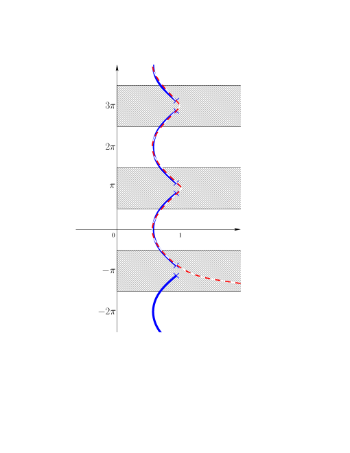
Figure 3: The contour of the integration which we consider (the dashed line) and cuts of the resolvent (the bold line) in polar coordinate. There are infinite number of the cuts and these cuts give the different contribution to the partition function each other. We take the beginning of the contour in the region $-\frac{3}{2}\pi<\arg x<-\frac{1}{2}\pi$ and $|x|\to\infty$, and the end of the contour in the region $\arg x\to\infty$. The integration picks up all cuts in the region $(2n-1)\pi<\arg x<(2n+1)\pi$ for $n\geq 0$. The cut with $n=0$ gives the contribution corresponding to the perturbative series of the $c=1$ noncritical string theory. The cuts with $n\geq 1$ correspond to the nonperturbative effect.

There is no local maximum in the effective potential for the Penner model except for what comes from the cut of the resolvent. However, the effective potential is multivalued on the complex plane of the $N$-th eigenvalue $x$, due to the logarithmic term of the potential. So, we use a polar coordinate on which the effective potential becomes single-valued. When we extend the range of $\theta=\arg x$ to $-\infty<\theta<+\infty$, there is a cut for each additional $2\pi$ of $\theta$. These infinite number of the cuts can be counted as the “saddle point” of the effective potential. For the Penner model, we usually assume that boundary terms of the integration with respect to the eigenvalues vanish. In the case for negative $g$, each end of the contour should be in the region in which $|x|\to\infty$ and $\mathop{\mathrm{Re}}x<0$. When, the range of $\theta$ is extended to $(-\infty,+\infty)$, each end of contour can be at any of $|x|\to\infty$ in shaded region of Fig 3 ($\left(2n+\tfrac{1}{2}\right)\pi<\theta<\left(2n+\tfrac{3}{2}\right)\pi$ with $n=\cdots,-2,-1.0,1,2,\cdots$). To make the model correspond to the $c=1$ noncritical string theory, we should add a small imaginary part to $g$, as we have seen in previous section. Then, boundary terms vanish at $\theta\to\infty$. We put the beginning of the contour at $|x|\to\infty$ in one of the shaded region of Fig 3, and the end of the contour at $\theta\to\infty$ (Fig 3). This contour picks up the cut which lies in the region where $\theta$ is greater than the beginning of the contour. The dominant contribution comes from the cut with the lowest value of the effective potential, which is located at the smallest $\theta$ of all the cuts along the contour, and the other cuts give sub-dominant contributions.

Now, we calculate the dominant contribution and nonperturbative corrections to the free energy of the Penner model. First, integrating the effective potential for the $N$-th eigenvalue, we calculate the nonperturbative correction from the configuration in which one eigenvalue is instanton. The effective potential can be written as

$$\mathrm{e}^{-NV_{\text{eff}}(x)}=\sum_{n=0}^{N}\psi_{n}^{2}(x),$$ (4.3)

where $\prod_{n}h_{n}$ is omitted because it does not depend on $x$. In the large $N$ limit, the orthonormal function $\psi_{n}(x)$ is constant on the cut up to sub-leading order, because $\psi_{n}(x)$ can be expressed as (4.2). We call the cut located in the region $(2k-1)\pi<\theta<(2k+1)$ $k$-th cut and denote it by $\mathcal{C}_{k}$. We define the value of $G_{\xi}(x)$ on these cuts as

$$\xi G_{\xi}(x_{k}) \equiv\bar{G}_{k}(\xi)=\text{const.}, \text{for }x_{k}\in\mathcal{C}_{k}.$$ (4.4)

Because the orthogonal polynomials $P_{n}(x)$ are single valued on the complex plane of $x$, the orthonormal functions $\psi_{n}(x)$ become multivalued via the potential of the Penner model $V(x)$. Therefore, the next to leading order corrections in $\frac{1}{N}$ of $\psi_{n}(x)$ is single valued. In fact, we can see that the $\mathcal{O}(N^{0})$ contribution of the orthogonal polynomials are single valued, via their concrete expression in the large $N$ limit (see appendix). Then, integrating the effective potential, we obtain,

$$\int\mathrm{d}x\,\mathrm{e}^{-NV_{\text{eff}}(x)} =\int\mathrm{d}x\sum_{n=0}^{N}\psi_{n}^{2}(x)$$

$$=\sum_{n=0}^{N}\sum_{k=0}^{\infty}\int_{\mathcal{C}_{0}}\mathrm{d}x\,\psi_{n}^{2}(x) =\sum_{n=0}^{N}\sum_{k=0}^{\infty}\mathrm{e}^{-N\left[\bar{G}_{k}(\frac{n}{N})-\bar{G}_{0}(\frac{n}{N})\right]}\int_{\mathcal{C}_{0}}\mathrm{d}x\,\psi_{n}^{2}(x).$$ (4.5)

Here, we define the normalization of the orthonormal functions in such a way that $\bar{G}_{0}=0$, namely,

$$\int_{\mathcal{C}_{0}}\mathrm{d}x\psi_{n}^{2}(x)=1.$$ (4.6)

To obtain the result corresponding to the $c=1$ noncritical string theory, we should take the suitable double scaling limit. We perform the rest of the calculation in this limit. We take the following limit,

$$g =-1+a^{2}t, x =-1+az, \xi =1-a^{2}\eta, N =a^{-2}.$$ (4.7)

In this limit, the difference of $G_{\xi}(x)$’s between two neighboring cuts becomes,

$$\bar{G}_{k+1}(\xi)-\bar{G}_{k}(\xi) =\int\mathrm{d}z\sqrt{z^{2}+4(t+\eta)}$$

$$=-2\pi i(t+\eta).$$ (4.8)

For the Penner model to correspond to the $c=1$ noncritical string theory, we should take $t=i\mu$, and it becomes $\bar{G}_{k+1}(\xi)>\bar{G}_{k}(\xi)$. We choose the contour in such the way that we pick up the $k$-th cut from $k=0$ to $k\to\infty$ in the integration. The dominant contribution comes from the $0$-th cut, because the $\bar{G}_{k}(\xi)$ is smallest for smallest $k$. Contributions from other cuts of $k\geq 1$ are contributions from instantons. Then, the dominant contribution, or the contribution from the configuration without the instanton, of the integration of the effective potential becomes

$$\int_{\text{inside the dominant cut}}\mathrm{d}x\mathrm{e}^{-NV_{\text{eff}}(x)}=\sum_{n}\int_{\mathcal{C}_{0}}\mathrm{d}x\psi_{n}^{2}(x)=N.$$ (4.9)

by replacing the summation over n by an integration, the contributions from instantons are

$$\int_{\text{inside sub-dominant cuts}}\mathrm{d}x\mathrm{e}^{-NV_{\text{eff}}(x)} =N\sum_{k=1}^{\infty}\sum_{n}\mathrm{e}^{2\pi i(t+\eta)k}$$

$$\simeq N^{2}a^{2}\sum_{k}\int\mathrm{d}\eta\mathrm{e}^{2\pi i(t+\eta)k}$$

$$=-N\sum_{k}\frac{1}{2\pi ik}\mathrm{e}^{2\pi itk}.$$ (4.10)

Here, the summation over $n$ is replaced by the integration over $\eta$. We also introduced some regularization to suppress the contribution from the terms with $\eta\gg 1$, because the double scaling limit does not work well in the region $\eta\gg 1$ and the terms with $\eta\gg 1$ is expected to be nonuniversal. Using (4.9), (4.10) and $t=i\mu$, we obtain

$$\delta F=\frac{Z^{\text{(1-inst)}}}{Z^{\text{(0-inst)}}}=-\sum_{k}\frac{1}{2\pi ik}\mathrm{e}^{-2\pi\mu k}.$$ (4.11)

But there is further correction to (4.10) which comes from the fact that we replace the summation over $n$ by an integration over $\eta$. This correction can be derived via the Euler-Mclaurin summation formula. Including this correction, prefactors of these terms diverge. To see this divergence, we introduce a regularization. When integrating over $\eta$ in (4.10), We have introduced some regularization, for example,

$$N\sum_{k}\int\mathrm{d}\eta\,\mathrm{e}^{2\pi i(t+\Lambda\eta)k}.$$ (4.12)

We first take $\mathop{\mathrm{Im}}\Lambda>0$, and after the integration, we take the limit of $\Lambda\to 1$. Now, we return the integration over $\eta$ to the summation. Then, $\eta$ can be regarded as integer, and it can be written as

$$\int_{\text{inside sub-dominant cuts}}\mathrm{d}x\mathrm{e}^{-NV_{\text{eff}}(x)} \simeq N\sum_{k}\sum_{\eta=0}^{\infty}\mathrm{e}^{2\pi i(t+\Lambda\eta)k}$$

$$=N\sum_{k}\frac{1}{1-\mathrm{e}^{2\pi i\Lambda k}}\mathrm{e}^{2\pi itk}.$$ (4.13)

Then, taking $\Lambda=1+\epsilon$, we obtain

$$\delta F=\frac{Z^{\text{(1-inst)}}}{Z^{\text{(0-inst)}}}=-\sum_{k}\frac{1}{2\pi i\epsilon k}\mathrm{e}^{-2\pi\mu k}.$$ (4.14)

Therefore, in the limit of $\epsilon\to 0$, the prefactors are diverge. We discuss this point later.

Up to now, we have simply considered the correction to the free energy from instantons to be $\delta F=\frac{Z^{(\text{1-inst})}}{Z^{(\text{0-inst})}}$. This is because we have ignored interactions between instantons, and we obtain

$$\frac{Z^{(n\text{-inst})}}{Z^{(\text{0-inst})}}\simeq{}_{N}C_{n}\left(\frac{\int_{\text{inside sub-dominant cuts}}\mathrm{d}x\left\langle\det\left(x-\Phi\right)^{2}\right\rangle\mathrm{e}^{-NV(x)}}{\int_{\text{inside the dominant cut}}\mathrm{d}x\left\langle\det\left(x-\Phi\right)^{2}\right\rangle\mathrm{e}^{-NV(x)}}\right)^{n}.$$ (4.15)

Then, the partition function can be written as

$$Z \simeq\lim_{N\to\infty}Z^{(\text{0-inst})}\left(1+\frac{1}{N}\frac{Z^{(\text{1-inst})}}{Z^{(\text{0-inst})}}\right)^{N}$$

$$=\mathrm{e}^{F^{(\text{0-inst})}+\frac{Z^{(\text{1-inst})}}{Z^{(\text{0-inst})}}}.$$ (4.16)

Therefore, the contribution from instantons to the free energy can be written as $\delta F=\frac{Z^{(\text{1-inst})}}{Z^{(\text{0-inst})}}$ approximately. To be exact, however, there are interactions between instantons, and we should include these effect. We consider multi-instanton effects in more detail.

To derive the effective potential of multiple eigenvalues, we use a slightly different method from that in [4]. The partition function of the matrix model can be written as

$$Z=\int\prod_{i=1}^{N}\mathrm{d}\lambda\,\Delta^{2}(\lambda)\,\mathrm{e}^{-N\sum_{i}V(\lambda_{i})}.$$ (4.17)

Here, the Vandermonde determinant $\Delta(\lambda)$ can be expressed in terms of the orthogonal polynomials as

$$\Delta(\lambda)=\det_{mn}P_{n-1}(\lambda_{m}).$$ (4.18)

Using this expression we can obtain the effective potential. First, we consider the effective potential of one eigenvalue. Integrating out the other eigenvalues than the $N$-th eigenvalue $x=\lambda_{N}$, we obtain

$$Z=(N-1)!\prod_{n=0}^{N-1}h_{n}\int\mathrm{d}x\,\sum_{n=0}^{N-1}\psi_{n}^{2}(\lambda).$$ (4.19)

This agrees with (4.1). Next, we consider the case in which two of eigenvalues are instantons. Integrating out $N-2$ eigenvalues, excluding $x=\lambda_{N}$ and $y=\lambda_{N-1}$, we obtain

$$Z=(N-2)!\prod_{n=0}^{N-1}h_{n}\int\mathrm{d}x\,\mathrm{d}y\,\sum_{n\neq m}\left(\psi_{n}^{2}(x)\,\psi_{m}^{2}(y)-\psi_{n}(x)\psi_{n}(y)\psi_{m}(x)\psi_{m}(y)\right).$$ (4.20)

Here, the second term can be dropped because this term vanishes due to the orthogonality of the orthogonal polynomials. Then, the contribution to the partition function from the configuration in which two of eigenvalues are the instanton becomes

$$Z^{(\text{2-inst})}=N!\prod_{n=0}^{N-1}h_{n}\int_{\text{inside sub-dominant cuts}}\mathrm{d}x\,\mathrm{d}y\sum_{n>m}\psi_{n}^{2}(x)\psi_{m}^{2}(y),$$ (4.21)

where we include the factor of ${}_{N}C_{2}$, which reflects the number of way of specifying two isolated eigenvalues. we can calculate the contribution from the configuration in which $l$ eigenvalues are instanton in a similar way. It can be written as

$$Z^{(l\text{-inst})}=N!\prod_{n=0}^{N-1}h_{n}\int_{\text{inside sub-dominant cuts}}\prod_{i=1}^{l}\mathrm{d}x_{i}\sum_{n_{1}>n_{2}>\cdots>n_{l}}\prod_{i=1}^{l}\psi_{n_{i}}^{2}(x_{i}).$$ (4.22)

By summing up these contributions, the partition function can be written as

$$Z =Z^{(\text{0-inst})}+Z^{(\text{1-inst})}+Z^{(\text{2-inst})}+\cdots$$

$$=N!\prod_{n=0}^{N-1}h_{n}\prod_{m=0}^{N-1}\left(1+\int_{\text{inside sub-dominant cuts}}\mathrm{d}x\,\psi_{m}^{2}(x)\right).$$ (4.23)

Then, we calculate this using concrete expressions of the orthonormal functions. We also use the regularization which is introduced in (4.12). Using (4.13), we obtain

$$Z=N!\prod_{n=0}^{N-1}h_{n}\prod_{m=0}^{N-1}\left(1+\sum_{k=1}^{\infty}\mathrm{e}^{2\pi i(t+\Lambda\eta(m))k}\right).$$ (4.24)

The free energy can be obtained by exponentiating this partition function:

$$\delta F =\sum_{\eta=0}^{\infty}\log\left[1+\sum_{k=1}^{\infty}\mathrm{e}^{2\pi i(t+\Lambda\eta)k}\right]$$

$$=\sum_{\eta=0}^{\infty}\log\left[\frac{1}{1-\mathrm{e}^{2\pi i(t+\Lambda\eta)}}\right]$$

$$=\sum_{\eta=0}^{\infty}\sum_{l=0}^{\infty}\frac{1}{l}\mathrm{e}^{2\pi i(t+\Lambda\eta)l}$$

$$=\sum_{l=1}^{\infty}\frac{1}{l\left(1-\mathrm{e}^{2\pi i\Lambda l}\right)}\mathrm{e}^{2\pi itl}.$$ (4.25)

Taking $t=i\mu$, we obtain

$$\delta F=\sum_{l=1}^{\infty}\frac{1}{l\left(1-\mathrm{e}^{2\pi i\Lambda l}\right)}\mathrm{e}^{-2\pi\mu l}.$$ (4.26)

Furthermore, we take $\Lambda=1+\epsilon$. Then, $\delta F$ can be written as

$$\delta F=\sum_{l=1}^{\infty}-\frac{1}{2\pi i\epsilon l^{2}}\mathrm{e}^{-2\pi\mu l}.$$ (4.27)

In the limit of $\epsilon\to 0$, the prefactors are diverge.

It is known that nonperturbative corrections of the $c=1$ noncritical string theory compactified on the circle with radius $R$ are given by terms of the form $\mathrm{e}^{-2\pi\mu k}$ and $\mathrm{e}^{-2\pi\mu kR}$ with positive integer $k$. Our result agrees with these forms. Another special feature of $\delta F$ is that prefactors of these terms diverge. To make the comparison of prefactors with those of the nonperturbative effect of the $c=1$ noncritical string theory, we use not the worldsheet formulation (the Liouville theory) but the matrix quantum mechanics formulation. The free energy of the $c=1$ noncritical string theory with radius $R$ can be obtained via the matrix quantum mechanics and expressed as [11, 12]

$$F=-\frac{1}{4}\int\frac{\mathrm{d}s}{s}\frac{\mathrm{e}^{i\mu s}}{\sinh\frac{s}{2}\sinh\frac{s}{2R}}.$$ (4.28)

Taking the contour to be the whole real axis, we obtain

$$F=i\sum_{n}\frac{\mathrm{e}^{-2\pi n\mu}}{4n(-1)^{n}\sin\left(\frac{\pi n}{R}\right)}+i\sum_{n}\frac{\mathrm{e}^{-2\pi nR\mu}}{4n(-1)^{n}\sin\left(\pi Rn\right)}$$ (4.29)

These terms come from the residues at the two series of poles $s=2\pi in$ and $s=2\pi inR$. There are two types of nonperturbative effects. The first term which comes from the poles $s=2\pi in$ doesn’t depend on the radius $R$ at leading order of the perturbative expansion. This term corresponds to the effect due to the D-instanton. On the other hand, the second term which comes from the poles $s=2\pi inR$ depends on the radius $R$ at the leading order of the perturbative expansion. This term corresponds to the effect due to the D-particle which is not localized in the direction compactified on the circle with radius $R$. For the self-dual radius of $R=1$, prefactors of these terms diverge individually. However, the whole is regular because these divergences cancel each other. Therefore the instantons of the Penner model correspond to only one of these two types of the nonperturbative effect. In fact, the expression with regularization (4.26) is quite similar to the individual terms of (4.29). These two terms cannot be distinguished for $R=1$. Someone may think that it is more similar to the first term of (4.29), but it depends on how to take the regularization. We cannot see which corresponds to the effect of instantons in the Penner model.

5 Conclusion

In this paper, we have studied the correspondence between the effects of the instantons in the Penner model and the nonperturbative effects in the $c=1$ noncritical string theory with self-dual radius. We have calculated the contribution from the instantons to the free energy of the Penner model. In the cases of the model corresponding to the $c=0$ noncritical string theory and kazakov series in the $c<1$ noncritical string theory, the instantons in hermitian one-matrix model are studied in recent works. The effects of the instantons agree with the nonperturbative effects of the noncritical string theory in these cases. In this paper, we have compared the effect of the instantons in the Penner model with the nonperturbative effect of the $c=1$ noncritical string theory compactified on the circle with self-dual radius of $R=1$.

In the case of the Penner model, especially in the double scaling limit corresponding to the $c=1$ noncritical string theory, the eigenvalues can no longer regarded as real. To make the model well-defined, we should introduce an analytic continuation. We have extended the definition of the Penner model, and defined the partition function as a multiple contour integral with respect to the $N$ eigenvalues. We have also found the suitable choice of the both ends of the contour that gives the effect of instantons corresponding to the nonperturbative effect of the $c=1$ noncritical string theory. In the case of the $c=0$ matrix model, the instanton is defined as the configuration with an eigenvalue on the local maximum of the effective potential. In the case of the Penner model, there are no local maxima of the effective potential. There are infinite number of cuts. In this case, the instanton is defined as an eigenvalue is located on the other cut along the contour than that corresponding to the perturbative series. In this way, we have generalized the calculation for the instantons to the Penner model.

Thus, we have seen the correspondence between the effects of the instanton and nonperturbative effects of the $c=1$ noncritical string theory at the leading order. The evaluation of the next-to-leading order fixes the prefactors of the contribution from the instantons. In the Penner model, these prefactors diverge. On the other hand, in the $c=1$ noncritical string theory with self-dual radius of $R=1$, the prefactors of the nonperturbative effect, which is calculated in the matrix quantum mechanics, do not diverge. However, the nonperturbative effects of the $c=1$ noncritical string theory is constructed from the effects that come from the D-instantons and D-particles. If we pick up the effects of the D-instantons only or D-particles only, the prefactor diverges. Therefore, the divergence of the prefactor does not mean the inconsistency of the correspondence. Furthermore, using the expression in which we introduce a regularization, we can find a similarity between our result and nonperturbative corrections which is calculated in the matrix quantum mechanics. For the self-dual radius of $R=1$, we cannot distinguish these effects that come from D-instantons and those from D-particles. Although we cannot specify which of D-instanton or D-particle corresponds to the instantons in the Penner model, there should be the effect corresponding to the other. And including this, we will obtain the prefactor which doesn’t diverge. This is left for future studies.

Acknowledgements:

The authors are grateful to H. Kawai for valuable advice and discussions. We would also like to thank M. Hanada for fruitful discussions. This work is supported in part by the Grant-in-Aid for Scientific Research (17$\cdot$1647) and the Grant-in-Aid for the 21st Century COE “Center for Diversity and Universality in Physics” from the Ministry of Education, Culture, Sports, Science and Technology (MEXT) of Japan. The work of Y.M. is supported in part by JSPS Research Fellowships for Young Scientists.

Appendix A Orthogonal polynomials in the Penner model

The method of orthogonal polynomials is a powerful tool to study the hermitian one-matrix model. In this section, we consider the orthogonal polynomials in the large $N$ limit for the Penner model.

Orthogonal polynomials $P_{n}(x)=x^{n}+\mathcal{O}(x^{n-1})$ is defined to obey the following orthogonal condition:

$$\left(P_{n},P_{m}\right)=\int\mathrm{d}x\ P_{n}(x)P_{m}(x)\mathrm{e}^{-NV(x)}=h_{n}\delta_{nm}.$$ (3.2)

The partition function of the hermitian one-matrix model is obtained via the recursion relation

$$xP_{n}(x) =X_{nm}P_{m}(x)=P_{n+1}(x)+s_{n}P_{n}(x)+r_{n}P_{n-1}(x),$$ (3.4a)

$$P_{n}^{\prime}(x) =\mathcal{P}_{nm}P_{m}(x)=\left[NV^{\prime}(X)\right]_{nm}P_{m}(x),$$ (3.4b)

where $r_{n}=\frac{h_{n}}{h_{n-1}}$. In the case of the Penner model, we take the potential $V(x)=\frac{1}{g}\left(x-\log x\right)$, and using (3.4b), we obtain

$$r_{n} =g\xi(g\xi+1),$$ (A.1a)

$$s_{n} =1+2g\xi+\frac{g}{N},$$ (A.1b)

where $\xi=\frac{n}{N}$. Using the ratio of the orthogonal polynomials $\mathrm{e}^{k_{n}}=\frac{P_{n}(x)}{P_{n-1}(x)}$, (3.4a) can be expressed as

$$x=\mathrm{e}^{k_{n+1}}+s_{n}+r_{n}\mathrm{e}^{-k_{n}}.$$ (A.2)

In the large $N$ limit, the rescaled index $\frac{n}{N}$ becomes a continuous variable $\xi$ and $k_{n}$ becomes continuous function $k(\xi)$. Then, we can expand $k$ as

$$k_{n+1} =k(\xi+\frac{1}{N})=k(\xi)+\frac{1}{N}\partial_{\xi}k(\xi)+\cdots,$$ (A.3a)

$$k_{n} =k_{n}^{(0)}+\frac{1}{N}k_{n}^{(1)}+\cdots.$$ (A.3b)

In a similar fashion, we expand $r_{n}$ and $s_{n}$ as

$$r_{n} =r(\xi)=g\xi(g\xi+1),$$ (A.4a)

$$s_{n} =s(\xi)=s_{n}^{(0)}+\frac{1}{N}s_{n}^{(1)},$$ (A.4b)

$$s_{n}^{(0)} =s^{(0)}(\xi)=1+2g\xi,$$ (A.4c)

$$s_{n}^{(1)} =s^{(1)}(\xi)=g=\frac{1}{2}\partial_{\xi}s^{(0)}(\xi).$$ (A.4d)

Substituting these relation to (A.2), we obtain

$$x =\mathrm{e}^{k_{n}^{(0)}}+s_{n}^{(0)}+r_{n}\mathrm{e}^{-k_{n}^{(0)}},$$ (A.5a)

$$0 =\left(k_{n}^{(1)}+\partial_{\xi}k_{n}^{(0)}\right)\mathrm{e}^{k_{n}^{(0)}}+\frac{1}{2}\partial_{\xi}s_{n}^{(0)}-r_{n}k_{n}^{(1)}\mathrm{e}^{-k_{n}^{(0)}}.$$ (A.5b)

Using these relation, we obtain

$$\mathrm{e}^{k_{n}^{(0)}} =\frac{1}{2}\left(x-(1+2g\xi)\pm\sqrt{x^{2}-2(1+2g\xi)x+1}\right),$$ (A.6a)

$$k_{n}^{(1)} =-\frac{1}{4}\partial_{\xi}\log\left[x^{2}-2(1+2g\xi)x+1\right].$$ (A.6b)

The sign of $\pm$ is taken to be $\mathrm{e}^{k_{n}}\sim x$ at $|x|\to\infty$. The orthogonal polynomials can be expressed as

$$P_{n}(x)=\exp\left[\sum_{m=1}^{n}k_{m}\right].$$ (A.7)

By using the Euler-Maclaurin summation formula to convert a summation into an integral, it becomes

$$P_{n}(x)=\exp\left[N\int_{0+\frac{1}{2N}}^{\xi+\frac{1}{2N}}\mathrm{d}\xi^{\prime}k(\xi^{\prime})\right].$$ (A.8)

The orthonormal functions $\psi_{n}(x)$ is convenient to describe the $n$-dependence of these functions. They can be expressed as

$$\psi_{n}(x)=\exp\left[-\frac{N}{2}V(x)+N\int_{0+\frac{1}{2N}}^{\xi+\frac{1}{2N}}\mathrm{d}\xi^{\prime}\left(k(\xi^{\prime})-\frac{1}{2}\log r(\xi^{\prime})\right)\right].$$ (A.9)

Then, substituting (A.6), we obtain

$$\psi_{n}(x) =\left[\frac{\left(x-(1+2g\xi)+\sqrt{x^{2}-2(1+2g\xi)x+1}\right)^{2}}{4g\xi(g\xi+1)\left(x^{2}-2(1+2g\xi)x+1\right)}\right]^{\frac{1}{4}}\exp\left[-\frac{N\xi}{2}G_{\xi}(x)\right],$$ (A.10a)

$$g\xi G_{\xi}(x) =-(1+2g\xi)\log\left[\frac{1}{2}\left(x-(1+2g\xi)+\sqrt{x^{2}-2(1+2g\xi)x+1}\right)\right]$$

$$\qquad-\log\left[\frac{1}{2}\left(x+1+\sqrt{x^{2}-2(1+2g\xi)x+1}\right)\right]$$

$$\qquad+\log\left[\frac{1}{2}\left(x-1+\sqrt{x^{2}-2(1+2g\xi)x+1}\right)\right]$$

$$\qquad+\sqrt{x^{2}-2(1+2g\xi)x+1}-2g\xi.$$ (A.10b)

The orthogonal polynomials $P_{n}(x)$ are single valued on the complex plane of $x$. However, its asymptotic form in the large $N$ limit has a cut. The presence of a cut indicate that the asymptotic form of the orthogonal polynomials is not single valued. This cut is only the consequence of the large $N$ limit. We should take the branch which reproduce the suitable form of the orthogonal polynomials in the large $N$ limit. The cut in the asymptotic form of the orthogonal polynomials is identical to that of the resolvent. We should take the physical sheet on which the resolvent becomes $R(x)\to\frac{1}{x}$ at $x\to\infty$ to obtain the suitable branch of the asymptotic behavior of the orthogonal polynomials. The orthogonal polynomials can be expressed in terms of the expectation value of the matrix model as

$$P_{n} =\left\langle\det\left(x-\Phi\right)\right\rangle_{n}$$

$$=\exp\left[\left\langle\mathop{\mathrm{tr}}\log\left(x-\Phi\right)\right\rangle_{c,n}+\cdots\right].$$ (A.11)

Here, the subscript “$n$” indicates that the expectation value is taken in the $n\times n$ matrix model, and the subscript $c$ indicates connected part. Then, in the large $N$ limit, the orthogonal polynomials can be expressed in terms of the resolvent $R(x)$ as

$$P_{n}(x)\simeq\exp\left[N\xi\int^{x}\mathrm{d}x^{\prime}R_{\xi}(x^{\prime})\right],$$ (A.12)

where $R_{\xi}(x)$ is the resolvent with the coupling of the matrix model $g$ replaced by $g\xi$. In fact, (A.10) shows that $P_{n}(x)$ behaves as

$$P_{n}(x)\simeq\exp\left[N\int_{0}^{\xi}\mathrm{d}\xi^{\prime}k^{(0)}(\xi^{\prime})\right]$$ (A.13)

at the leading order, and using the relation

$$\partial_{x}\int_{0}^{\xi}\mathrm{d}\xi^{\prime}k^{(0)}(\xi^{\prime}) =\pm\int_{0}^{\xi}\frac{\mathrm{d}\xi^{\prime}}{\sqrt{x^{2}-2(1+2g\xi^{\prime})x+1}}$$

$$=\pm\frac{1}{2gx}\left[\sqrt{x^{2}-2(1+2g\xi)x+1}-|x-1|\right]=\xi R_{\xi}(x),$$ (A.14)

we can see the agreement with (A.12). The sign included in the expression of $k$ should be taken to be the same as the resolvent. The resolvent becomes $R(x)\sim\frac{1}{x}$ in the limit $x\to\infty$ on the physical sheet. Then, the orthogonal polynomials behave as

$$P_{n}(x)\sim\exp\left[N\xi\int^{x}\mathrm{d}x^{\prime}\frac{1}{x^{\prime}}\right]=x^{n}.$$ (A.15)

It reproduces the suitable behavior of the orthogonal polynomials in the limit of $x\to\infty$. It also corresponds to that the sign of $\pm$ is taken to be $\mathrm{e}^{k_{n}}\sim x$ at $|x|\to\infty$ in (A.6).

On the cut, the orthogonal polynomials can be obtained as a linear combination of two branches corresponding to, for instance, the $+$ and $-$ in the sign of $\pm$ in the (A.6). It is explained as follows. When we consider the orthonormal function $\psi_{n}(x)=\frac{1}{\sqrt{h_{n}}}P_{n}(x)\mathrm{e}^{-\frac{N}{2}V(x)}$, in the large $N$ limit, it becomes

$$\psi_{n}(x)\sim\exp\left[-\frac{N\xi}{2}\mathop{\mathrm{Re}}G_{\xi}(x)\right]\sin[\frac{N\xi}{2}\mathop{\mathrm{Im}}G_{\xi}(x)+\frac{\pi}{4}].$$ (A.16)

Since the imaginary part of the $G(x)$ is the density of eigenvalues and $G_{\xi}(x)$ is obtained from $G(x)$ by replacing $g$ with $g\xi$, the orthonormal functions and orthogonal polynomials have the point where $P_{n}(x)=\psi_{n}(x)=0$ on the cut. The orthogonal polynomials can be expressed in terms of the expectation value of the matrix model as

$$P_{n}(x) =\left\langle\det\left(x-\Phi\right)\right\rangle_{n}$$

$$=\left\langle\prod_{i=1}^{n}(x-\lambda_{i})\right\rangle.$$ (A.17)

Then, in the large $N$ limit, it becomes $P_{n}(x)=0$ at the point where an eigenvalue is classically located. Because the cut of the resolvent comes from the support of the eigenvalue distribution, the point where $P_{n}(x)=0$ is on the cut. To obtain the point where $P_{n}(x)=\psi_{n}(x)=0$, we should take the linear combination of two branches. Meanwhile, the oscillatory behavior of $\psi_{n}^{2}(x)$ can be approximated by the average of $\frac{1}{2}$ and we can regard it as a constant inside the cut.

We can see how to take the linear combination of two branches of the asymptotic form of the orthogonal polynomials by studying the behavior near the endpoint of the cut. In this region, the orthogonal polynomials can be approximated by the Airy function. In the double scaling limit, the orthonormal functions become

$$\psi_{n}\sim\exp\left[-\frac{1}{2}\int\mathrm{d}z\sqrt{z^{2}+4(t+\eta)}\right].$$ (A.18)

The recursion relation that the orthogonal polynomials satisfy gives the differential equation which the orthonormal functions satisfy in the double scaling limit. The differential equation for the orthonormal functions at the leading order of the perturbative expansion of the noncritical string is

$$\frac{\partial^{2}\psi_{n}}{\partial z^{2}}=\frac{1}{4}(z^{2}+4t)\psi_{n}(z).$$ (A.19)

The both ends of the cut is located on $z=\pm 2i\sqrt{t}$. Introducing the new variable $y$ and $\theta$ defined by $z=2i\sqrt{t}+\mathrm{e}^{i\theta}y$, we obtain a differential equation,

$$\frac{\partial^{2}\psi_{n}(y)}{\partial y^{2}}+a\mathrm{e}^{3i\vartheta\frac{\pi}{2}i}y\psi_{n}(y).$$ (A.20)

Then, for $\theta=\frac{\pi}{6},\,-\frac{\pi}{2},\cdots$, we can make use of a standard analysis of the Airy function. This implies that the cut is on the line of $\theta=\frac{\pi}{6},\,-\frac{\pi}{2},\cdots$. It corresponds to the condition that the cut is on the line on which $G(x)$ is pure imaginary. The other condition that the cut is embedded on the region where $G(x)\leq 0$ determines that the cut is on the line of the $\theta=\frac{\pi}{6}$. The Airy function can be expressed via the integration on the complex plane of $k$ as

$$\psi(y)=\int\mathrm{d}k\ \exp\left[yk+\frac{1}{3}k^{3}\right].$$ (A.21)

The asymptotic form of the Airy function can be obtained by the method of the steepest descent. There are two saddle points in the $k$ plane, corresponding to the two branches of the asymptotic form of the orthogonal polynomials. For $\theta=\frac{\pi}{6}$ and $y>0$, we take the contour which picks up the both of two saddle points. This corresponds to the linear combination of the two branches. Then, for $y<0$, this contour picks up only one of the saddle point. So we shouldn’t take the linear combination in this region. The contour of the integration is determined by the choice of the boundary of the contour. We should use the same choice of the boundary for $\theta=-\frac{\pi}{2}$. Since the saddle points are placed at the different point from the case of $\theta=\frac{\pi}{6}$, this contour picks up only one of the saddle point for both $y>0$ and $y<0$. In this way, we should take the linear combination of two branches only inside the cut.

The orthonormal functions $\psi_{n}(x)=\frac{1}{\sqrt{h_{n}}}P_{n}(x)\mathrm{e}^{-\frac{N}{2}V(x)}$ obey the following orthonormality condition:

$$\int\mathrm{d}x\ \psi_{n}(x)\psi_{m}(x)=\delta_{nm}.$$ (A.22)

Here, the integration with respect to $x$ can be approximated by the integration inside the cut in the large $N$ limit. We check (A.10) satisfies this orthonormality condition, especially the normalization. First, the orthonormal function given by (A.10) becomes

$$\psi_{n}(x)\sim\exp[N\int_{0}^{\xi}\mathrm{d}\xi^{\prime}\left(k^{(0)}(\xi^{\prime})-\frac{1}{2}\log r(\xi^{\prime})\right)]$$ (A.23)

at the leading order of the $\frac{1}{N}$ expansion. When we take the average of the oscillatory behavior of the square of the orthonormal functions $\psi_{n}^{2}(x)$, it can be regarded as a constant on the cut. Examining on the end of the cut $x=x_{0}(\xi)$, we find $k^{(0)}(\xi)-\frac{1}{2}\log r(\xi)=0$. Here, the position of the cut depends on the index of $n$ of the orthogonal polynomials. Then, $n$-dependence of the $\psi_{n}^{2}(x)$ becomes

$$\frac{\mathrm{d}\psi_{n}^{2}(x_{0})}{\mathrm{d}\xi}\sim 2N\left(k^{(0)}(\xi)-\frac{1}{2}\log r(\xi)\right)\psi_{n}^{2}(x_{0})=0.$$ (A.24)

The norm of the orthonormal function $\psi_{n}(x)$ does not depend on $n$ at the leading order of the $\frac{1}{N}$ expansion.

Second, on the correction at the order of $\frac{1}{N}$, we have the following expression for the orthonormal function $\psi_{n}(x)$:

$$\psi_{n}^{2}(x)=\frac{x-(1+2g\xi)+\sqrt{x^{2}-2(1+2g\xi)x+1}}{2\sqrt{x^{2}-2(1+2g\xi)x+1}\sqrt{g\xi(g\xi+1)}}\mathrm{e}^{\mathcal{O}(N)}.$$ (A.25)

Here, the $\mathcal{O}(N)$ contribution can be neglected, because it does not depend on $n$ as we have seen earlier. Using this expression and integrating inside the cut, we obtain

$$\int\mathrm{d}x\psi_{n}^{2}(x)=1.$$ (A.26)

Therefore, $\psi_{n}(x)$ obeys suitable normalization condition defined by the integration inside the cut.

Appendix B The universality in the Penner model

Generally, in the double scaling limit, the quantities describing the physics of the noncritical string do not depend on the details of the potential of the matrix model. This universality reflects the fact that the physical quantities do not depend on the cut-off. Conversely speaking, the universal quantity which does not depend on the details of the potential is physical quantity of the noncritical string theory.

We can introduce the universality into the Penner model. In the case of the Penner model, we can add arbitrary polynomials into the potential. Generally, we can consider the following potential:

$$V(x)=\frac{1}{g}\left(\sum_{k=1}^{l}\frac{g_{k}}{k}x^{k}-\log x\right).$$ (B.1)

When we consider the Penner model as the model corresponding to the $c=1$ noncritical string theory, we restrict ourselves to the critical point on which two ends of the cut merge. On such critical point, $r_{n}$ in (3.4a) takes the value $r_{c}=0$. In the double scaling limit, that is the $N\to\infty$ with

$$g =g_{c}(1-a^{2}t), x =x_{c}+az, \xi =1-a^{2}\eta, N =a^{-2},$$ (B.2)

$r_{n}$ and $s_{n}$ defined in (3.4a) becomes

$$r_{n} =-a^{2}\alpha\ (t+\eta)+\mathcal{O}(a^{4}),$$ (B.3a)

$$s_{n} =x_{c}+a^{2}\beta\ (t+\eta)+\mathcal{O}(a^{4}).$$ (B.3b)

The resolvent can be described in terms of the orthogonal polynomials as

$$R(x) =\int_{0}^{1}\mathrm{d}\xi\oint\frac{\mathrm{d}\omega}{\omega}\frac{1}{\omega+s(\xi)+r(\xi)\,\omega^{-1}}$$

$$\simeq\int\frac{\mathrm{d}\eta}{\sqrt{z^{2}+4\alpha\ (t+\eta)}}$$

$$=\frac{1}{2\alpha}\sqrt{z^{2}+4\alpha\ (t+\eta)}.$$ (B.4)

Then, $\bar{G}_{k}(\xi)$ in this case becomes

$$\bar{G}_{k+1}(\xi)-\bar{G}_{k}(\xi) =\int\mathrm{d}z\frac{1}{\alpha}\sqrt{z^{2}+4\alpha\ (t+\eta)}$$

$$=-2\pi i(t+\eta).$$ (B.5)

It agrees with the result for the usual Penner model (4.8). We can do the rest of the calculation in the same way as the usual Penner model. Then, we obtain the same result for the contribution from the instantons.

References

- [1] P. Di Francesco, P. H. Ginsparg and J. Zinn-Justin, “2-D Gravity and random matrices,” Phys. Rept. 254 (1995) 1 [arXiv:hep-th/9306153].
- [2] P. H. Ginsparg and G. W. Moore, “Lectures on 2-D gravity and 2-D string theory,” arXiv:hep-th/9304011.
- [3] I. R. Klebanov, “String theory in two-dimensions,” arXiv:hep-th/9108019.
- [4] M. Hanada, M. Hayakawa, N. Ishibashi, H. Kawai, T. Kuroki, Y. Matsuo and T. Tada, “Loops versus matrices: The nonperturbative aspects of noncritical string,” Prog. Theor. Phys. 112, 131 (2004) [arXiv:hep-th/0405076].
- [5] H. Kawai, T. Kuroki and Y. Matsuo, “Universality of nonperturbative effect in type 0 string theory,” Nucl. Phys. B 711 (2005) 253 [arXiv:hep-th/0412004].
- [6] A. Sato and A. Tsuchiya, “ZZ brane amplitudes from matrix models,” JHEP 0502 0502 (2005) 032 [arXiv:hep-th/0412201].
- [7] N. Ishibashi, T. Kuroki and A. Yamaguchi, “Universality of nonperturbative effects in c ¡ 1 noncritical string theory,” JHEP 0509 (2005) 043 [arXiv:hep-th/0507263].
- [8] J. Distler and C. Vafa, “A Critical Matrix Model At C = 1,” HUTP-90-A062
- [9] S. Chaudhuri, H. Dykstra and J. D. Lykken, “The Penner matrix model and C = 1 strings,” FERMILAB-PUB-91-049-T
- [10] J. Ambjorn, C. F. Kristjansen and Y. Makeenko, “Generalized Penner models to all genera,” Phys. Rev. D 50 (1994) 5193 [arXiv:hep-th/9403024].
- [11] S. Y. Alexandrov, V. A. Kazakov and D. Kutasov, “Non-perturbative effects in matrix models and D-branes,” JHEP 0309 (2003) 057 [arXiv:hep-th/0306177].
- [12] S. Y. Alexandrov and I. K. Kostov, “Time-dependent backgrounds of 2D string theory: Non-perturbative effects,” JHEP 0502 (2005) 023 [arXiv:hep-th/0412223].