YITP-SB-05-44
hep-th/0512101

Half-BPS Geometries and
Thermodynamics of Free Fermions

Simone Giombi, Manuela Kulaxizi,
Riccardo Ricci and Diego Trancanelli

C. N. Yang Institute for Theoretical Physics
State University of New York at Stony Brook
Stony Brook, NY 11794-3840, USA

ABSTRACT

Solutions of type IIB supergravity which preserve half of the supersymmetries have a dual description in terms of free fermions, as elucidated by the “bubbling AdS” construction of Lin, Lunin and Maldacena. In this paper we study the half-BPS geometry associated with a gas of free fermions in thermodynamic equilibrium obeying the Fermi-Dirac distribution. We consider both regimes of low and high temperature. In the former case, we present a detailed computation of the ADM mass of the supergravity solution and find agreement with the thermal energy of the fermions. The solution has a naked null singularity and, by general arguments, is expected to develop a finite area horizon once stringy corrections are included. By introducing a stretched horizon, we propose a way to match the entropy of the fermions with the entropy of the geometry in the low temperature regime. In the opposite limit of high temperature, the solution resembles a dilute gas of D3 branes. Also in this case the ADM mass of the geometry agrees with the thermal energy of the fermions.

1 Introduction

According to the AdS/CFT correspondence, deformations of AdS geometries should map to states in the dual CFT living at the boundary of AdS [1]. Recently a concrete realization of this map has been found for the important sector of half-BPS operators of ${\cal N}=4$ Super Yang-Mills. These operators have conformal dimension $\Delta$ equal to the $U(1)_{R}$ charge. They form a decoupled sector of ${\cal N}=4$ Super Yang-Mills which can be efficiently described by a gauged quantum mechanics matrix model with harmonic oscillator potential, see [2] and for earlier work [3]. The matrix model is well known to be completely integrable. The main reason behind integrability is that, in the eigenvalue basis, the eigenvalues behave as fermions in a harmonic potential. In the semiclassical limit the half-BPS states can be depicted as droplets of fermions in a two-dimensional phase space. One expects then the following AdS/CFT dictionary. Small ripples above the Fermi sea correspond to graviton excitations of $AdS_{5}\times S^{5}$. Small holes below the Fermi energy correspond to giant gravitons, while small droplets of fermions outside the Fermi sea map to dual giant gravitons. All this is very reminiscent of both old and recent works on $c=1$ string theory and its matrix model reinterpretation [4] [5] (for a recent review see [6]).

Remarkably this whole picture has found an impressive confirmation through the explicit construction of the full moduli space of half-BPS IIB supergravity solutions discovered by Lin, Lunin and Maldacena (LLM) [7] . The phase space distribution of the matrix model eigenvalues is in one-to-one correspondence with IIB supergravity backgrounds which preserve half of the supersymmetry. Moreover the two-dimensional phase space of the fermions has an interesting physical embedding in the space-time geometry. At the quantum level the incompressibility of the droplets in phase space (due to Fermi-Dirac statistics) corresponds in the dual supergravity side to the requirement that the Ramond-Ramond five-form flux is quantized. The whole family of half-BPS geometries can be constructed in terms of an auxiliary function $z$ which also determines the fermion distribution. The regularity of the supergravity background amounts to requiring a suitable boundary condition on the auxiliary function. The AdS “bubbling geometries” are therefore in general smooth supergravity backgrounds.

The fermions discussed so far are characterized by having a step-function distribution in the two-dimensional phase space. They can be seen therefore as fermions at zero “temperature”. It is then natural to investigate how turning on the temperature affects the supergravity solution. The fermion at non zero temperature are described by a Fermi-Dirac distribution. The corresponding AdS “bubbling” solution has been first obtained in [9] and further studied in [10] where it was given the name of hyperstar. This supergravity background can be thought of as resulting from a coarse graining process of smooth half-BPS geometries. The fermion distribution of the hyperstar fails to satisfy the boundary conditions necessary to obtain a smooth gravity solution. Quite generally when the smoothness condition is not satisfied naked singularities occur [11] [12]. One expects that $\alpha^{\prime}$ string corrections will modify the geometry in proximity of the singularity and that a horizon will be generated [13] [14]. This class of singular supergravity solution can therefore be regarded as incipient black holes. An example of singular LLM solution is the superstar [15], which has been investigated from this point of view in [16] [17].

The duality between fermion distributions and supergravity solutions at zero temperature suggests that the thermodynamic properties of the fermion gas at finite temperature should agree with the corresponding quantities in the supergravity side. In particular, one expects agreement between the thermal excitation energy of the fermions and the ADM mass of the supergravity solution. We will check that this is indeed the case in the two opposite regimes of low and high temperature.

As we have already remarked, the hyperstar geometry is singular. The singularity is resolved quantum mechanically through the appearance of a finite area horizon. One can then use the Bekenstein-Hawking formula to compute the associated entropy. By placing a stretched horizon in the hyperstar geometry we propose a way to match the supergravity entropy with the thermal entropy of the fermions in the low temperature regime, up to a numerical factor.

Similarly we investigate the opposite regime of high temperature. In this limit the Fermi-Dirac distribution reduces to the classical Boltzmann distribution. We find that in this regime the metric is reminiscent of the so called dilute gas limit of LLM configurations associated to the Coulomb branch of Super Yang-Mills.

The organization of the paper is the following. In the next section we present a concise description of the main results of LLM. In sec. 3 we review the thermodynamics of 1D fermions in a harmonic potential. In sec. 4 we introduce the hyperstar geometry, discuss its properties in the low temperature regime, compute the ADM energy, angular momentum and entropy and we compare the results to the fermion prediction. In sec. 5 we move on to consider the high temperature limit of the hyperstar distribution, we find the corresponding metric and determine its mass and angular momentum. We conclude discussing some open questions in sec. 6.

2 Review of LLM

In this paragraph we briefly review the LLM construction [7] of $1/2$ BPS IIB supergravity backgrounds. These solutions correspond, in the dual CFT side, to states satisfying the BPS condition

$$\Delta=J$$ (1)

where $\Delta$ is the corresponding conformal dimension and $J$ is a particular $U(1)$ charge of the $SO(6)$ R-symmetry group. By selecting one generator of the $SO(6)$ R-symmetry group of ${\cal N}=4$ Super Yang-Mills we obtain a theory with $SO(4)\times SO(4)\times R$ bosonic symmetry. In the dual supergravity description we look therefore for solutions with this isometry group. Assuming that axion and dilaton are constant and that only the self-dual five-form field strength is turned on, the Ansatz for the background is

$$ds^{2} = g_{\mu\nu}dx^{\mu}dx^{\nu}+e^{H+G}d\Omega_{3}^{2}+e^{H-G}d{\tilde{\Omega}}_{3}^{2}$$ (2)

$$F_{(5)} = F_{\mu\nu}dx^{\mu}\wedge dx^{\nu}\wedge d\Omega_{3}+{\tilde{F}}_{\mu\nu}dx^{\mu}\wedge dx^{\nu}\wedge d{\tilde{\Omega}}_{3}$$ (3)

where the Greek indices $\mu,\nu$ run over $0,\ldots,3$. The two three-spheres $S^{3}$ and $\tilde{S}^{3}$ in the metric make the $SO(4)\times SO(4)$ isometries manifest. The additional $R$ isometry corresponds to the Hamiltonian $\Delta-J$.

For a background to be half-BPS there should exist a solution to the Killing spinor equation. Analyzing this equation, LLM were able to prove that the generic 1/2 BPS IIB supergravity background takes the form

$$ds^{2} = -h^{-2}(dt+V_{i}dx^{i})^{2}+h^{2}(dy^{2}+dx^{i}dx^{i})+ye^{G}d\Omega_{3}^{2}+ye^{-G}d\tilde{\Omega}_{3}^{2}$$ (4)

$$h^{-2} = 2y\cosh G,$$ (5)

$$y\partial_{y}V_{i} = \epsilon_{ij}\partial_{j}z,\;\;\;\;\;\;\;\;\;\;y(\partial_{i}V_{j}-\partial_{j}V_{i})=\epsilon_{ij}\partial_{y}z$$ (6)

$$z = \frac{1}{2}\tanh G$$ (7)

$$F = dB_{t}\wedge(dt+V)+B_{t}dV+d\hat{B}~{},~{}~{}~{}~{}~{}~{}$$

$$\tilde{F} = d\tilde{B}_{t}\wedge(dt+V)+\tilde{B}_{t}dV+d\hat{\tilde{B}}$$ (8)

$$B_{t} = -\frac{1}{4}y^{2}e^{2G},~{}~{}~{}~{}~{}~{}~{}~{}~{}~{}~{}~{}~{}~{}~{}~{}~{}~{}\tilde{B}_{t}=-\frac{1}{4}y^{2}e^{-2G}$$ (9)

$$d\hat{B} = -\frac{1}{4}y^{3}*_{3}d\left(\frac{z+\frac{1}{2}}{y^{2}}\right)~{},~{}~{}~{}~{}~{}~{}~{}~{}d\hat{\tilde{B}}=-\frac{1}{4}y^{3}*_{3}d\left(\frac{z-\frac{1}{2}}{y^{2}}\right)$$ (10)

where $i=1,2$ and $\star_{3}$ is the Hodge dual operator for the flat three-dimensional space parameterized by $x_{1},x_{2},y$. Remarkably, the solution is completely specified in terms of a single auxiliary function $z(x_{1},x_{2},y)$ which satisfies the linear differential equation

$$\partial_{i}\partial_{i}z+y\partial_{y}\left(\frac{\partial_{y}z}{y}\right)=0.$$ (11)

It is important to note that at $y$ equals zero the product of the radii of the two privileged three-spheres is zero. Therefore, to avoid singular geometries, the auxiliary function $z$ must satisfy a suitable boundary condition. This smoothness condition turns out to be $z=\pm\frac{1}{2}$ on the boundary plane $y=0$. In the limit $z\rightarrow 1/2$ the $\tilde{S}^{3}$ sphere shrinks to zero while the other three-sphere remains finite. The reverse statement applies when $z\rightarrow-1/2$. It is conventional to assign black and white colors respectively to the $z=-1/2$ and $z=1/2$ points in the $(x_{1},x_{2})$ plane. If $\cal{D}$ denotes a black region in this plane, the energy of the associated supergravity solution has the simple expression

$$\Delta=J=\int_{\cal{D}}\frac{d^{2}x}{2\pi\hbar}\ \frac{1}{2}\frac{(x_{1}^{2}+x_{2}^{2})}{\hbar}-\frac{1}{2}\left(\int_{\cal{D}}\frac{d^{2}x}{2\pi h}\right)^{2}\,.$$ (12)

The ${\mathbb{R}}^{2}$ plane has then a natural interpretation as the phase space of one-dimensional fermions in a harmonic potential. This nicely matches the matrix model description in the dual CFT side [2]. It emerges a beautiful picture of the moduli space of half-BPS geometries of IIB supergravity in terms of configurations of droplets of fermions on the $(x_{1},x_{2})$ plane. Note that the fundamental equation (11) has the symmetry $z\rightarrow-z$ which simply exchanges the $S^{3}$ and $\tilde{S}^{3}$ in the solution. In a field theory description of the fermions, this symmetry amounts to a particle-hole duality.

The quantization condition on the total area $\cal{A}$ of the droplets is related to the five-form flux $N$ as follows

$$\frac{{\cal A}}{2\pi\hbar}=N$$ (13)

with

$$\hbar=2\pi l_{p}^{4}.$$ (14)

The flux $N$ coincides with the number of fermions. The simplest configuration in phase space is a black circular droplet of radius $R_{0}=\sqrt{2\hbar N}$ and the associated geometry is $AdS_{5}\times S^{5}$ with $N$ units of the five-form flux. This background has $\Delta=J=0$ and corresponds to the fermion ground state. The boundary of the droplet can be thought of as the Fermi level of the fermions. The $S^{5}$ of the background is obtained by fibering the $\tilde{S}^{3}$ sphere on a two-dimensional surface $\Sigma_{2}$ in the $(x_{1},x_{2},y)$ space which encircles the droplet. One can easily obtain configurations with an arbitrary number of $S^{5}$’s by adding other droplets. If we deform the circular droplet to configurations with different shapes but same area, we obtain backgrounds with $AdS_{5}\times S^{5}$ asymptotics.

The fundamental equation (11) can be rewritten as a Laplace equation for the quantity $\Phi=z/y^{2}$ in a six-dimensional space with spherical symmetry in four of the coordinates. The coordinate $y$ corresponds to the radial direction in the four-dimensional subspace. This observation reduces the task of finding the full solution $z(x_{1},x_{2},y)$ of eq. (11) to a well known initial-value problem. Once the boundary condition $z(x_{1},x_{2},0)$ on the $y=0$ plane is specified, the solution is

$$z(x_{1},x_{2},y)=\frac{y^{2}}{\pi}\int_{\mathbb{R}^{2}}\frac{z(x_{1}^{\prime},x_{2}^{\prime},0)dx_{1}^{\prime}dx_{2}^{\prime}}{[({\bf{x-x^{\prime}}})^{2}+y^{2}]^{2}}.$$ (15)

We can similarly get

$$V_{i}(x_{1},x_{2},y)=\frac{\epsilon_{ij}}{\pi}\int_{\mathbb{R}^{2}}\frac{z(x_{1}^{\prime},x_{2}^{\prime},0)(x_{j}-x_{j}^{\prime})dx_{1}^{\prime}dx_{2}^{\prime}}{[({\bf{x-x^{\prime}}})^{2}+y^{2}]^{2}}.$$ (16)

Since we are going to consider only droplet configurations with radial symmetry, it will be convenient to rewrite the above formulas in polar coordinates $(x_{1},x_{2})\rightarrow(R,\phi)$. It is easy to see that in this case $V_{R}=V_{1}\cos\phi+V_{2}\sin\phi=0$. Defining $V\equiv V_{\phi}=R(-V_{1}\sin\phi+V_{2}\cos\phi)$ the differential equations relating $z$ and $V$ (6) read

$$y\,\partial_{y}\,V\,=\,-R\,\partial_{R}\,z\,,~{}~{}~{}~{}~{}~{}~{}~{}~{}~{}~{}\frac{1}{R}\,\partial_{R}\,V\,=\,\frac{1}{y}\,\partial_{y}\,z.$$ (17)

Rewriting eq. (15) and eq. (16) in polar coordinates yields

$$z(R,y)=-\int z(R^{\prime},0)\frac{\partial}{\partial R^{\prime}}z_{0}(R,y;R^{\prime})dR^{\prime}$$ (18)

$$V(R,y)=\int z(R^{\prime},0)g_{V}(R,y;R^{\prime})dR^{\prime}$$ (19)

where

$$z_{0}(R,y;R^{\prime}) = \frac{R^{2}-R^{\prime 2}+y^{2}}{2\left[(R^{2}+R^{\prime 2}+y^{2})^{2}-4R^{2}R^{\prime 2}\right]^{1/2}}$$ (20)

$$g_{V}(R,y;R^{\prime}) = \frac{-2R^{2}R^{\prime}(R^{2}-R^{\prime 2}+y^{2})}{\left[(R^{2}+R^{\prime 2}+y^{2})^{2}-4R^{2}R^{\prime 2}\right]^{3/2}}.$$ (21)

We remark that $z_{0}$ is the LLM function corresponding to a circular droplet. Indeed in this case $z(R^{\prime},0)=1/2\,\mbox{Sign}(R^{\prime}-R_{0})$ and using eq. (18) one obtains $z(R,y)=z_{0}(R,y;R_{0})$. As previously anticipated such a configuration gives rise to the $AdS_{5}\times S^{5}$ solution. In fact performing the following change of coordinates [7]

$$y = R_{0}\sinh\rho\sin\theta$$ (22)

$$R = R_{0}\cosh\rho\cos\theta$$ (23)

$$\phi = \tilde{\phi}+t$$ (24)

one recovers the $AdS_{5}\times S^{5}$ metric in standard form

$$ds^{2}=R_{0}\big{(}-\cosh^{2}\rho dt^{2}+d\rho^{2}+\sinh^{2}\rho d\Omega_{3}^{2}+d\theta^{2}+\cos^{2}\theta d\tilde{\phi}^{2}+\sin^{2}\theta d\tilde{\Omega}_{3}^{2}\big{)}.$$ (25)

A variation of the method described so far can be similarly applied to obtain 1/2 BPS M-theory backgrounds with $AdS_{4,7}\times S^{7,4}$ asymptotics [7]. In this case the geometry is in one-to-one correspondence with solutions of a three-dimensional Toda equation, which plays the same role as eq. (11).

3 1D fermions in the harmonic well

In this section we review the basics of the thermodynamics of one-dimensional fermions in a harmonic potential. In what follows, we will consistently adopt units in which $\hbar=k_{B}=1$. We consider a gas of $N$ non-interacting fermions with hamiltonian

$$H(p,q)=\frac{1}{2}(p^{2}+q^{2})$$ (26)

in thermodynamic equilibrium at a given temperature $T$. For large $N$, we adopt the semi-classical approximation in which the energy is taken to be a continuous variable. The probability distribution as a function of the energy $H(p,q)=\epsilon$ is given by the Fermi-Dirac distribution:

$$n_{FD}(\epsilon)=\frac{1}{e^{(\epsilon-\mu)/T}+1}$$ (27)

where $\mu$ is the Fermi energy. This is determined by the normalization condition

$$\int_{0}^{\infty}\frac{d\epsilon}{e^{(\epsilon-\mu)/T}+1}=N$$ (28)

which gives

$$\mu=T\ln(e^{N/T}-1).$$ (29)

We will first consider the limit of very small temperature $T$, or more precisely $N/T\gg 1$. In this limit, the Fermi level becomes

$$\mu=N+\mathcal{O}(Te^{-N/T}).$$ (30)

The total energy of the Fermi gas is given by:

$$E=\int_{0}^{\infty}\frac{\epsilon\,d\epsilon}{e^{(\epsilon-\mu)/T}+1}$$ (31)

which for small $T$ can be evaluated by means of the Sommerfeld expansion [18]

$$I=\int_{0}^{\infty}\frac{f(\epsilon)d\epsilon}{e^{(\epsilon-\mu)/T}+1}=\int_{0}^{\mu}f(\epsilon)d\epsilon+\frac{\pi^{2}}{6}T^{2}f^{\prime}(\mu)+\frac{7\pi^{4}}{360}T^{4}f^{\prime\prime\prime}(\mu)+\mathcal{O}(T^{6}).$$ (32)

This gives:

$$E\simeq\frac{N^{2}}{2}+\frac{\pi^{2}}{6}T^{2}.$$ (33)

The first term is clearly the ground state energy of the $N$ fermions, so we expect the dual gravity solution to have a mass (and angular momentum) difference of $\Delta=\frac{\pi^{2}}{6}T^{2}$ with respect to the $AdS_{5}\times S^{5}$ background. It is worth noting that in eq. (33) we only neglect exponentially suppressed terms. In fact, since $f(\epsilon)=\epsilon$, there are no power series corrections to the energy beyond $T^{2}$. This is a specific feature of the 1D harmonic oscillator, and we will recover it in the energy and angular momentum of the hyperstar in the low $T$ limit.

To evaluate the entropy of the fermion gas, it is convenient to first obtain the free-energy $F$ of the system. This is computed from the partition function $Z$, which in the continuous limit we are considering reads

$$Z=\mbox{exp}\left[-{N\mu\over T}+\int_{0}^{\infty}d\epsilon\,\ln(1+e^{-(\epsilon-\mu)/T})\right].$$ (34)

One can verify that this expression for the partition function is correct by checking that the relation $E=-{\partial\over\partial\beta}\ln Z$ (where $\beta=1/T$) is satisfied. Using the definition $F=-T\ln Z$ one obtains the free energy

$$F = N\mu-T\int_{0}^{\infty}d\epsilon\,\ln(1+e^{-(\epsilon-\mu)/T})$$ (35)

$$= N\mu-\int_{0}^{\infty}d\epsilon\,{\epsilon\over e^{(\epsilon-\mu)/T}+1}=N\mu-E$$ (36)

where in the second line an integration by parts was made. The entropy is then given by the relation $F=E-TS$ from which we get

$$S=\frac{2E-N\mu}{T}.$$ (37)

For small $T$, using eq. (30) and eq. (33) one gets

$$S\simeq\frac{\pi^{2}}{3}T$$ (38)

where again only exponetially small terms are neglected.

We now consider the opposite limit of very high temperature $N/T\ll 1$. In this limit, the Fermi distribution clearly reduces to the Boltzmann density

$$n_{FD}(\epsilon)\rightarrow n_{B}(\epsilon)=N\beta\,e^{-\beta\epsilon}$$ (39)

where $\beta=1/T$. The total energy in this approximation is readily computed

$$E=NT.$$ (40)

The entropy can be obtained from eq. (37) (which is valid for any temperature) using the large $T$ approximation

$$\mu\simeq T\ln N/T$$ (41)

and reads

$$S\simeq N\ln T+2N-N\ln N.$$ (42)

4 The hyperstar: Low temperature regime

We now introduce the half-BPS geometry dual to the Fermi-Dirac gas described in the previous section [9]. This solution was named hyperstar in [10].

A given $z(R,0)$ corresponds to a fermion density $n(R)$ in the phase space via the relation

$$z(R,0)=\frac{1}{2}-n(R).$$ (43)

For example, the $AdS_{5}\times S^{5}$ solution is associated to the step function density $n_{0}=\vartheta(R-R_{0})$, which can be viewed as the zero temperature limit of the Fermi-Dirac distribution (27). One can turn on the temperature on the fermion side by replacing $n_{0}$ with $n_{FD}(R)$ and construct the corresponding supergravity background by using (18), (19) and (43). It is important to remark that the temperature we are turning on is the temperature in the “auxiliary” description of the free fermion gas. It is not a temperature of the supergravity solution or of the dual gauge theory. Indeed, we remain in the supersymmetric half-BPS sector. It would be interesting to understand better what corresponds to this temperature on the gravity and gauge theory side. For the time being, we regard $T$ just as a deformation parameter of the $AdS_{5}\times S^{5}$ background.

For low temperatures, the solution is a small perturbation of the circular droplet. In fact in this limit the fermion configuration in the $(x_{1},x_{2})$ looks like a black disk with the boundary slightly “blurred”, as shown in fig. 1.

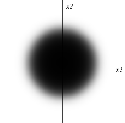
Figure 1: Droplet configuration in the low temperature limit. The greyscale ring around the Fermi level corresponds to a singular region of the spacetime.

In the low temperature limit the expressions (18) and (19) can be obtained analytically as follows [9]

$$z^{T}_{FD}(R,y) = \frac{1}{2}+\int_{0}^{\infty}n_{FD}(R^{\prime})\frac{\partial}{\partial R^{\prime}}z_{0}(R,y;R^{\prime})dR^{\prime}$$ (44)

$$= z_{0}(R,y;R_{0})+\frac{\pi^{2}}{6}T^{2}\left[\frac{\partial^{2}}{\partial\epsilon^{2}}z_{0}(R,y;R_{0}=\sqrt{2\epsilon})\right]_{\epsilon=\frac{R_{0}^{2}}{2}}+\mathcal{O}(T^{4})$$ (45)

and

$$V^{T}_{FD}(R,y) = -\int_{0}^{\infty}n_{FD}(R^{\prime})g_{V}(R,y;R^{\prime})dR^{\prime}$$ (46)

$$= V_{0}(R,y;R_{0})-\frac{\pi^{2}}{6}T^{2}\left[\frac{\partial}{\partial\epsilon}\left(\frac{g_{V}(R,y;R_{0}=\sqrt{2\epsilon})}{\sqrt{2\epsilon}}\right)\right]_{\epsilon=\frac{R_{0}^{2}}{2}}+\mathcal{O}(T^{4})$$ (47)

where we have used the Sommerfeld expansion (32) and where

$$V_{0}(R,y;R_{0})=\frac{1}{2}\left(\frac{R^{2}+R_{0}^{2}+y^{2}}{\left[(R^{2}+R_{0}^{2}+y^{2})^{2}-4R^{2}R_{0}^{2}\right]^{1/2}}-1\right)$$ (48)

corresponds to the $AdS_{5}\times S^{5}$ background. In these expressions $R_{0}=\sqrt{2N}$ is the radius of the droplet in the phase space at $T=0$, and $N$ is the number of fermions. It is easy to check that (45) and (47) satisfy the differential equations (17).

4.0.1 ADM form of the metric

In order to compute the mass and the angular momentum associated to the hyperstar, it is convenient to perform the following change of coordinates

$$R = L^{2}\left(1+\frac{r^{2}}{L^{2}}\right)^{1/2}\cos\theta$$ (49)

$$y = L\,r\,\sin\theta$$ (50)

$$\phi = \tilde{\phi}+\frac{t}{L}$$ (51)

and we also rescale $t\rightarrow L\,t$ to have conventional units. Here $(t\,,\,r\,,\,\Omega_{3})$ parameterize the asymptotic $AdS_{5}$ (in global coordinates), whereas $(\theta\,,\,\tilde{\phi}\,,\,\tilde{\Omega}_{3})$ span the asymptotic $S^{5}$. Of course, $L$ is the radius of both the $AdS_{5}$ and the $S^{5}$. It is related to the radius $R_{0}$ used by [7] via $R_{0}=L^{2}$. In this system of coordinates the metric can be rewritten in ADM form as

$$ds^{2}=-\mathcal{N}^{2}dt^{2}+g_{\theta\theta}\left(\frac{dr^{2}}{r^{2}+L^{2}}+d\theta^{2}\right)+g_{\tilde{\phi}\tilde{\phi}}\left(d\tilde{\phi}+\mathcal{N}^{\tilde{\phi}}dt\right)^{2}+g_{\Omega_{3}\Omega_{3}}\ d\Omega_{3}^{2}+g_{\tilde{\Omega}_{3}\tilde{\Omega}_{3}}\ d\tilde{\Omega}_{3}^{2}$$ (52)

where $\mathcal{N}$ is the lapse function and $\mathcal{N}^{\tilde{\phi}}$ is the shift vector.

Introducing the expansion parameter

$$\gamma\equiv\frac{2\pi^{2}T^{2}}{3L^{8}}=\frac{\pi^{2}T^{2}}{6N^{2}}$$ (53)

and using the explicit expressions for $z^{T}_{FD}$ and $V^{T}_{FD}$

$$z^{T}_{FD}(R,y) = \frac{R^{2}-R_{0}^{2}+y^{2}}{2\left[(R^{2}+R_{0}^{2}+y^{2})^{2}-4R^{2}R_{0}^{2}\right]^{1/2}}+$$ (56)

$$+\frac{2R_{0}^{4}y^{2}\big{(}(R_{0}^{2}+y^{2})^{2}+R^{2}(R_{0}^{2}-y^{2})-2R^{4}\big{)}}{\left[(R^{2}+R_{0}^{2}+y^{2})^{2}-4R^{2}R_{0}^{2}\right]^{5/2}}\gamma+\mathcal{O}(\gamma^{2})$$

$$V^{T}_{FD}(R,y) = \frac{1}{2}\left(\frac{R^{2}+R_{0}^{2}+y^{2}}{\left[(R^{2}+R_{0}^{2}+y^{2})^{2}-4R^{2}R_{0}^{2}\right]^{1/2}}-1\right)+$$ (60)

$$+\frac{2R_{0}^{4}R^{2}\big{(}(R^{2}-R_{0}^{2})^{2}-y^{2}(R^{2}+R^{2}_{0}+2y^{2})\big{)}}{\left[(R^{2}+R_{0}^{2}+y^{2})^{2}-4R^{2}R_{0}^{2}\right]^{5/2}}\gamma+\mathcal{O}(\gamma^{2})$$

one obtains, upon implementing eq. (51), the components of the metric, which we present here up to $\mathcal{O}(\gamma^{2})$ terms

$$\mathcal{N}^{2} = \left(1+\frac{r^{2}}{L^{2}}\right)\,\Big{[}1-\gamma L^{2}F_{1}(r,\theta)\Big{]}\,,$$ (61)

$$\mathcal{N}^{\tilde{\phi}} = \gamma\frac{2L(r^{2}+L^{2})(r^{2}+L^{2}\cos^{2}\theta)}{(r^{2}+L^{2}\sin^{2}\theta)^{3}}\,,$$ (63)

$$g_{\tilde{\phi}\tilde{\phi}} = L^{2}\cos^{2}\theta\Big{[}1+\gamma L^{2}F_{1}(r,\theta)\Big{]}\,,$$ (65)

$$g_{\theta\theta} = L^{2}\left[1+\gamma L^{2}\frac{r^{2}-L^{2}\sin^{2}\theta}{r^{2}+L^{2}\sin^{2}\theta}F_{2}(r,\theta)\right]\,,$$ (67)

$$g_{\Omega_{3}\Omega_{3}} = r^{2}\Big{[}1-\gamma L^{2}F_{2}(r,\theta)\Big{]}\,,$$ (69)

$$g_{\tilde{\Omega}_{3}\tilde{\Omega}_{3}} = L^{2}\sin^{2}\theta\Big{[}1+\gamma L^{2}F_{2}(r,\theta)\Big{]}\,,$$ (71)

where

$$F_{1}(r,\theta) = \frac{(3\cos^{2}\theta-1)r^{4}+3L^{2}\cos^{4}\theta\,r^{2}+L^{4}(2\cos^{4}\theta+\sin^{2}\theta)}{(r^{2}+L^{2}\sin^{2}\theta)^{3}}\,,$$ (72)

$$F_{2}(r,\theta) = \frac{(3\cos^{2}\theta-1)r^{4}+L^{2}(3\cos^{4}\theta-2\sin^{2}\theta)r^{2}+L^{4}(2\cos^{4}\theta-\cos^{2}\theta-1)}{(r^{2}+L^{2}\sin^{2}\theta)^{3}}\,$$ (74)

A general property of LLM distributions with compact support is that the corresponding geometries are asymptotically $AdS_{5}\times S^{5}$. One can check that this remains true for the metric eq. (71). This is consistent with the fact that the droplet of fig. 1 is effectively confined in a finite region of the phase space. From the expressions in (74), we also notice that the Sommerfeld expansion seems no longer reliable in a region around the point $r=\theta=0$. The appearance of eventual singularities will be discussed in the following section.

4.0.2 Singularity

The study of singularities for LLM geometries was undertaken in [11] and [12] . There it was shown that all singularities appearing in the LLM supergravity solutions are naked and fall into two classes, namely timelike and null. While the former are considered highly pathological due to the presence of closed timelike curves, the latter are not. In fact, for half-BPS geometries with null singularity, the underlying fermion density function $n(R)$ always takes values in the region $n(R)\in(0,1)$. This is the case both for the hyperstar and the superstar solutions.

To verify the presence of a singularity in the geometry, one should find a curvature invariant which diverges. The first non trivial invariant to consider is $R^{2}_{MN}=R_{MN}R^{MN}$, $(M,N=0,\ldots,9)$, since the Ricci scalar $R$ vanishes. Indeed, as a result of the Weyl invariance of the classical theory, the trace of the matter stress-tensor is identically zero. In order to check the consistency of the metric eq. (71) we explicitly verified that this is the case.

There are two ways to perform the computation of $R_{MN}^{2}$. The direct approach involves the explicit form of the metric, while the indirect one makes use of the field equations of type IIB supergravity. In this case, the knowledge of the five form field strength $F_{(5)}$ will suffice:

$$R_{MN}=\frac{1}{5!}\left(\frac{5}{2}F_{M}^{\;\;\;P_{1}P_{2}P_{3}P_{4}}F_{NP_{1}P_{2}P_{3}P_{4}}-\frac{1}{4}g_{MN}F^{2}\right).$$ (75)

Suppose now we use the approximate solution for the metric, whose explicit form was given in the previous section, eq. (71). A lengthy calculation gives

$$R^{2}_{MN}=\frac{160}{L^{4}}+\gamma\,\frac{P_{6}(r,\cos\theta)}{L^{2}(r^{2}+L^{2}\sin^{2}\theta)^{4}}+\mathcal{O}(\gamma^{2}).$$ (76)

In this $\gamma$ expansion, the first term corresponds to $AdS_{5}\times S^{5}$ and is, of course, finite. The linear term in $\gamma$ is, however, potentially divergent. Here $P_{6}(r,\cos\theta)$ is a sixth order polynomial in both $r$ and $\cos\theta$ and goes to zero as $(r^{2}+L^{2}\sin^{2}\theta)$ when $r\rightarrow 0$ and $\theta\rightarrow 0$. The square of the Ricci tensor is therefore divergent when $r=0$ and $\theta=0$. It is interesting to note here that this is exactly the singular behavior one sees in Kerr black holes. Due to their angular momentum, the collapsing region is not a point but a zero-thickness ring. The Kretschmann invariant $K\sim R_{MNRS}R^{MNRS}$, for instance, for a Kerr black hole with mass $M$ and angular momentum $J=Ma$, is

$$K=M^{2}\frac{Q_{6}(r,\cos\theta)}{(r^{2}+a^{2}\cos^{2}\theta)^{6}}$$ (77)

where $Q_{6}(r,\cos\theta)$ also indicates a sixth order polynomial having the same behavior as $P_{6}(r,\cos\theta)$ in the vicinity of $r=0$ and $\theta=0$. This is suggestive of the existence of an event horizon in the hyperstar geometry which may manifest itself through $\alpha^{\prime}$-corrections to the supergravity solution.

This is not however the result one would have anticipated. From the form of the metric in LLM coordinates, it is quite natural to expect a singularity at $y=0$. Using (51), we can see that this corresponds to $r=0$ or $\theta=0$ in asymptotic $AdS_{5}\times S^{5}$ coordinates. On the other hand, the singular region appearing in (76) is mapped to $(R=L,y=0)$, which is just the Fermi surface of the fermions. We expect the singularity to be at least smeared over an extended region around the Fermi energy, since there the fermion density is less than one, see fig. 1.

What is therefore the true singular region of the hyperstar? We can try to address this question in a quite general fashion valid for all LLM geometries. We simply need to know the behavior of the functions $z(R,y)$ and $V(R,y)$ in proximity of $y=0$. We can distinguish two different cases depending on whether $z_{0}(R,0)=\lim_{y\rightarrow 0}z(R,y)$ is independent of the radial coordinate $R$ or not. In what follows we will focus on the latter, since this is the case of the hyperstar.

We would like to find $z(R,y)$ and $V(R,y)$ in terms of an expansion in $y$ or functions of $y$, such that the differential equations (17) will be order by order satisfied. It turns out that the appropriate Ansatz is the following

$$z(R,y) = z_{0}(R,0)+f_{1}(R)\,y^{2}\,\ln y+\ldots$$ (78)

$$V(R,y) = V_{0}(R,0)+g_{1}(R)\,\ln y+\ldots$$ (79)

The functions $f_{i}(R)$ and $g_{i}(R)$ are determined to each order from the same differential equation (17). For the case that concerns us here we have $f_{1}(R)=-\frac{1}{2R}\partial_{R}(R\partial_{R}z_{0}(R,0))$, $V_{0}(R,0)=-\frac{1}{2}R\partial_{R}z_{0}$ and $g_{1}(R)=-R\partial_{R}z_{0}$. It is now easy to find the complete solution for the metric and the five-form field strength in this region and subsequently calculate $R^{2}_{MN}$, using either of the methods indicated above. We find

$$R^{2}_{MN}=\frac{h_{1}(z_{0}(R,0))}{y^{2}}+h_{2}(z_{0}(R,0),f_{1}(R))\,\ln y+\ldots$$ (80)

where $h_{1}(z_{0}(R,0))$ and $h_{2}(z_{0}(R,0),f_{1}(R))$ are non-zero functions of the variables indicated.

Indeed we see that the leading term is divergent at $y=0$, as expected. We must therefore conclude that this is the singular region of the hyperstar, and that we cannot rely on the Sommerfeld expansion (32) for calculations in the small $y$ region. This will be important later for computing the entropy through the Bekenstein-Hawking formula.

4.0.3 Flux

To check the consistency of the hyperstar solution, we can verify that the flux of the five form $F_{(5)}$ remains equal to $N$, independently from the temperature $T$ of the fermion gas. From general considerations this has to be expected, since the temperature can be viewed as a tunable continuous parameter and as such it cannot modify the flux which is a topological constraint. At zero temperature, i.e. for the $AdS_{5}\times S^{5}$ solution, using the explicit expressions for the field strength in the LLM solution and the change of coordinates eq. (51) one obtains

$$F^{(0)}_{(5)}=\frac{r^{3}}{L}\,dt\wedge dr\wedge d\Omega_{3}+2N\sin^{3}\theta\cos\theta\,d\theta\wedge d\tilde{\phi}\wedge d\tilde{\Omega}_{3}.$$ (81)

The flux is computed by integrating $F^{(0)}_{(5)\theta\tilde{\phi}\tilde{\Omega}_{3}}$ over the $S^{5}$, and including the appropriate normalization is equal to $N$. To check that temperature perturbations do not alter the flux, one has to verify that corrections to $F^{(0)}_{(5)\theta\tilde{\phi}\tilde{\Omega}_{3}}$ vanish when integrated over the five sphere. Up to second order in the temperature, these take the form

$$F^{(1)}_{(5)\theta\tilde{\phi}\tilde{\Omega}_{3}} = \gamma\,\sin^{3}\theta\cos\theta\,\frac{L^{6}\,p_{6}(r,\cos\theta)}{(r^{2}+L^{2}\sin^{2}\theta)^{4}}$$ (82)

$$F^{(2)}_{(5)\theta\tilde{\phi}\tilde{\Omega}_{3}} = \gamma^{2}\,\sin^{3}\theta\cos\theta\,\frac{L^{10}\,p_{10}(r,\cos\theta)}{(r^{2}+L^{2}\sin^{2}\theta)^{8}}$$ (83)

where $p_{6}$ and $p_{10}$ are polynomials of degree 6 and 10 respectively. Although the explicit formulas look rather involved, the integration over $\theta$ can be carried out exactly at arbitrary $r$ and indeed yields

$$\int_{0}^{\pi/2}d\theta\,F^{(1)}_{(5)\theta\tilde{\phi}\tilde{\Omega}_{3}}=\int_{0}^{\pi/2}d\theta\,F^{(2)}_{(5)\theta\tilde{\phi}\tilde{\Omega}_{3}}=0.$$ (84)

4.1 Mass

In this section we present a systematic derivation of the ADM mass of the hyperstar solution. The natural expectation is that this mass should coincide with the thermal energy of the auxiliary fermion gas system.

The Einstein-Hilbert action in a $d$-dimensional spacetime is

$$S_{grav}=\frac{1}{16\pi G_{d}}\int_{\mathcal{M}}d^{d}x\sqrt{-g}\,(R-2\Lambda)-\frac{1}{8\pi G_{d}}\oint_{\partial\mathcal{M}}d^{d-1}x\sqrt{-\gamma}\,\Theta$$ (85)

where we included the Gibbons-Hawking boundary term and $\gamma_{\mu\nu}$ is the metric on the $(d-1)$-dimensional timelike boundary. Following [19], the quasi-local stress-tensor can be computed by the variation of the gravitational action with respect to the boundary metric

$$T^{\mu\nu}={2\over\sqrt{-\gamma}}{\delta S_{grav}\over\delta\gamma_{\mu\nu}}.$$ (86)

Using (85) this is

$$T^{\mu\nu}={1\over 8\pi G_{d}}\left(\Theta^{\mu\nu}-\Theta\gamma^{\mu\nu}\right).$$ (87)

In the previous expression we have introduced the extrinsic curvature of the $(d-1)$-dimensional timelike boundary embedded in $\mathcal{M}$

$$\Theta^{\mu\nu}=-{1\over 2}\nabla_{(g)}^{(\mu}\hat{n}^{\nu)}$$ (88)

and we denoted the corresponding trace by $\Theta$. The covariant derivative is taken with respect to the metric $g_{\mu\nu}$ of the full spacetime and $\hat{n}^{\nu}$ is the unit normal to the boundary. The stress-tensor (86) generically diverges as we approach the boundary $\partial{\cal M}$ when the spacetime is asymptotically AdS. In the context of the AdS/CFT correspondence we can view the gravitational quasi-local stress-tensor as the expectation value of the stress-tensor in the associated conformal field theory. The divergences get then a natural interpretation as standard ultraviolet divergences in quantum field theory [20]. We can regularize the theory by adding suitable counterterms to the original stress-tensor

$$T^{\mu\nu}={1\over 8\pi G_{d}}\left(\Theta^{\mu\nu}-\Theta\gamma^{\mu\nu}+{2\over\sqrt{-\gamma}}{\delta S_{ct}\over\delta\gamma_{\mu\nu}}\right).$$ (89)

The counterterms are consistently constructed using only the boundary metric $\gamma_{\mu\nu}$ and its covariant derivatives and are (almost) uniquely determined by requiring a cancellation of the divergences and general covariance (for a review, see [21]). The boundary metric $\gamma_{\mu\nu}$ can be written in the ADM form

$$\gamma_{\mu\nu}dx^{\mu}dx^{\nu}=-\mathcal{N}^{2}_{\Sigma}dt^{2}+\sigma_{ab}(dx^{a}+\mathcal{N}^{a}_{\Sigma}dt)(dx^{b}+\mathcal{N}^{b}_{\Sigma}dt)$$ (90)

where $\Sigma$ is a surface of constant $t$ inside $\partial{\cal M}$. Conserved charges are obtained by integrating $T^{\mu\nu}$ over a spacelike hypersurface at infinity. A finite expression for the mass is obtained substituting the regularized stress-energy tensor in the following formula

$$M=\int_{\Sigma}d^{d-2}x\,\sqrt{\sigma}\mathcal{N}_{\Sigma}u^{\mu}T_{\mu\nu}u^{\nu},$$ (91)

where $u^{\mu}$ is the timelike unit normal to $\Sigma$. For instance, the application of this method to the five-dimensional AdS-Schwarzschild black hole

$$ds^{2}=-\left[{r^{2}\over L^{2}}+1-\left({r_{0}\over r}\right)^{2}\right]dt^{2}+{dr^{2}\over\left[{r^{2}\over L^{2}}+1-\left({r_{0}\over r}\right)^{2}\right]}+r^{2}(d\theta^{2}+\sin^{2}{\theta}d\phi^{2}+\cos^{2}{\theta}d\psi^{2})$$ (92)

yields [20]

$$M={3\pi l^{2}\over 32G_{5}}+{3\pi r_{0}^{2}\over 8G_{5}}.$$ (93)

The first term, which is present also when the black hole disappears, corresponds to the Casimir energy of the vacuum in the dual CFT.

It would be nice to have a similar counterterm method directly in a ten-dimensional setting. Unfortunately, extending the program of holographic renormalization to ten-dimensional metrics with $AdS_{5}\times S^{5}$ asymptotics seems problematic [22]. We are therefore forced to use alternative approaches. In the first one, we will determine the relevant components of the stress-tensor relative to some reference geometry following [23]. The second approach is the so called background subtraction method [24]. In both cases one has to carefully match the asymptotic geometry of the supergravity solution with that of a reference background. Neither of the methods can reproduce the Casimir energy of the associated CFT. However this will not be a problem in our case since we are interested in computing the energy difference between the half-BPS supergravity solution and the $AdS_{5}\times S^{5}$ ground state.

We now proceed to compute the mass of the hyperstar (71) as a series expansion in the small parameter $\gamma\equiv\frac{\pi^{2}T^{2}}{6N^{2}}$. This mass should agree with the energy of the free fermion gas, eq. (33). We will first consider the leading order in $\gamma$ and comment on $\gamma^{2}$ orders in a later section.

4.1.1 First approach

Following [23], we obtain the stress-tensor associated with the metric (71) relative to the $AdS_{5}\times S^{5}$ background metric $g^{0}_{\mu\nu}$. We need to require that the difference between the two metrics falls off suitably fast for large radius. Explicitly we want that

$$g_{rr}-g_{rr}^{0}=o(1/r^{6})$$ (94)

$$g_{ra}-g_{ra}^{0}=o(1/r^{5})$$ (95)

where $o(1/r^{n})$ means that these differences go to zero more rapidly than $1/r^{n}$ and the index $a$ runs over all the coordinates except $r$. To satisfy such requirement we implement an appropriate change of coordinates $(r,\theta)\rightarrow(\tilde{r},\tilde{\theta})$, which we presently discuss. The effect of using these new coordinates is to make the leading asymptotic perturbations of the metric all in components parallel to the boundary directions. Then the line element becomes

$$ds^{2}=g_{\mu\nu}^{0}dx^{\mu}dx^{\nu}+\frac{\hat{T}_{ab}}{\tilde{r}^{2}}dx^{a}dx^{b}+\ldots$$ (96)

from which one can read off the stress-tensor up to a multiplicative constant depending only on the space-time dimensions.

The first step is therefore to find a coordinate system such that the metric satisfies (95). We consider the Ansatz

$$r = \tilde{r}+\frac{f_{1}}{\tilde{r}}+\frac{f_{2}}{\tilde{r}^{3}}$$ (97)

$$\cos{\theta} = \cos{\tilde{\theta}}+\frac{f_{3}}{\tilde{r}^{2}}+\frac{f_{4}}{\tilde{r}^{4}}$$ (98)

where the $f_{i}=f_{i}(\tilde{\theta})$ $(i=1,\ldots,4)$ are functions to be determined in order to adjust the asymptotics of the metric.

In terms of the new variables $\tilde{r}$ and $\tilde{\theta}$, the $g_{\tilde{r}\tilde{r}}$ component of the metric has an expansion for large $\tilde{r}$ which differs from the background reference metric $g^{0}_{\tilde{r}\tilde{r}}=(1+\tilde{r}/L^{2})^{-1}$ by terms containing the $f_{i}$. The $1/\tilde{r}^{4}$ term can be eliminated by tuning $f_{1}=\frac{1}{4}(3\cos{\tilde{\theta}}^{2}-1)L^{2}\gamma$ and similarly the $1/\tilde{r}^{6}$ with an appropriate choice of $f_{2}$. The first constraint in (95) is then satisfied. Analogously, $f_{3}$ and $f_{4}$ are fixed by requiring the vanishing of the $1/\tilde{r}^{3}$ and $1/\tilde{r}^{5}$ terms in $g_{\tilde{r}\tilde{\theta}}$, which appears after changing variables according to (98). Once the $f_{i}$ are fixed, one can verify that the other components of the metric coincide with $g^{0}_{\mu\nu}$ up to orders $\mathcal{O}\left(\tilde{r}^{-2}\right)$. The only disagreement is found in $g_{tt}$ and $g_{\Omega_{3}\Omega_{3}}$, which contain a term at order $\mathcal{O}\left(\tilde{r}^{0}\right)$

$$\gamma(3\cos^{2}\tilde{\theta}-1)$$ (99)

which, nonetheless, vanishes upon integration over the $S^{5}$ (including the appropriate measure). We notice that the same factor already appeared at leading order in the asymptotic expansion of the metric perturbation, see eq. (74).

From (96) and the explicit expression for

$$g_{tt}=-\mathcal{N}^{2}+g_{\tilde{\phi}\tilde{\phi}}\left(\mathcal{N}^{\tilde{\phi}}\right)^{2}$$ (100)

one can read off the time-time component of the stress-tensor

$$\hat{T}_{tt} = \left(g_{tt}(\tilde{r},\tilde{\theta})+1+\frac{\tilde{r}^{2}}{L^{2}}\right)\tilde{r}^{2}$$ (101)

$$= \frac{\gamma}{8}\left(4(3\cos^{2}\tilde{\theta}-1)\tilde{r}^{2}+L^{2}\big{(}11-39\cos^{2}\tilde{\theta}+60\cos^{4}\tilde{\theta}\big{)}\right)+\mathcal{O}\left(\frac{1}{\tilde{r}^{2}}\right).$$ (103)

This expression has to be integrated at the spacelike boundary in order to give the mass

$$M = \frac{4}{16\pi G_{10}}\int\,\hat{\mu}\,\hat{T}_{tt}$$ (104)

$$= \frac{4}{16\pi G_{10}}L^{5}(2\pi)(2\pi^{2})^{2}\int_{0}^{\pi/2}d\theta\cos{\theta}\sin^{3}{\theta}\;\hat{T}_{tt}$$ (105)

where $G_{10}=\frac{\pi^{4}L^{8}}{2N^{2}}$ and $\hat{\mu}=\tilde{r}^{-3}\sqrt{g_{\tilde{\phi}\tilde{\phi}}\,g_{\theta\theta}\,g_{\Omega\Omega}^{3}\,g_{\tilde{\Omega}\tilde{\Omega}}^{3}}$ is the integration measure. The final result for the mass is

$$M=\frac{L^{7}}{4}\gamma=\frac{\pi^{2}}{6L}T^{2}$$ (106)

which agrees with the thermal excitation energy of the $N$ fermions above the ground state, eq. (33). The extra $L$ in the denominator comes from the rescaling of the time variable already discussed. It is important to remark that in obtaining these expressions we have consistently worked at order $\gamma$. We will comment on the significance of higher order terms in a later section.

4.1.2 The superstar

As a further check of the validity of the procedure just discussed, we also apply it to the so-called superstar, a family of asymptotically $AdS_{5}\times S^{5}$ backgrounds discovered in [15] and further studied from the LLM perspective in [16] [11] [17] [10]. The extremal 1/2 BPS superstar metric is governed by two parameters, the flux $N$ of the 5-form through the $S^{5}$ and one of the three angular momenta on the $S^{5}$, $J_{3}$, which coincides with the energy $\Delta$ because of the BPS condition. Explicitly the metric can be written as [11]

$$ds^{2} = -\frac{1}{G}\left(\cos^{2}\theta+\frac{r^{2}}{L^{2}}G^{2}\right)dt^{2}+\frac{L^{2}H}{G}\sin^{2}\theta d\phi^{2}+2\frac{L}{G}\sin^{2}\theta dtd\phi+$$ (109)

$$+G\left(\frac{dr^{2}}{f}+r^{2}d\Omega_{3}^{2}\right)+L^{2}Gd\theta^{2}+\frac{L^{2}}{G}\cos^{2}\theta d\tilde{\Omega}_{3}^{2}$$

with

$$f=1+H\frac{r^{2}}{L^{2}}\,,~{}~{}~{}~{}~{}~{}G=\sqrt{\sin^{2}\theta+H\cos^{2}\theta}\,,~{}~{}~{}~{}~{}H = 1+\frac{2L^{2}\Delta}{N^{2}r^{2}}\equiv 1+\frac{Q}{r^{2}}.$$ (110)

Also in this example we want to satisfy the fall off conditions (95). By choosing an appropriate coordinate system as in (98) it is easy to see that

$$\hat{T}_{tt} = \frac{Q}{4L^{2}}\big{(}2-3\cos^{2}\tilde{\theta}\big{)}^{2}\tilde{r}^{2}+$$ (113)

$$+\frac{Q}{64L^{2}}\big{(}(6-36\cos^{2}\tilde{\theta})L^{2}-(4+15\cos^{2}\tilde{\theta}-24\cos^{4}\tilde{\theta})Q\big{)}+\mathcal{O}\left(\frac{1}{\tilde{r}}\right).$$

The expression for the mass is then

$$M = \frac{4}{16\pi G_{10}}\int\,\hat{\mu}\,\hat{T}_{tt}=\frac{4}{16\pi G_{10}}L^{5}\pi^{5}Q=\frac{\Delta}{L}$$ (114)

which, up to the $L$ coming from the rescaling of the time, is exactly the energy of the geometry. Note that we have again neglected contributions quadratic in $Q$ in the stress-tensor (113).

4.1.3 Second approach: Background subtraction

We now discuss the second approach [24] for computing the mass of the hyperstar. In the background subtraction prescription the ADM mass is obtained by integrating the quasi-local energy ${\cal N}(K-K_{0})$ over the $(d-2)$-dimensional spacelike hypersurface $\Sigma$ at radial infinity

$$M=\frac{1}{8\pi G_{10}}\int_{\Sigma}\,\mu\,\mathcal{N}\,(K-K_{0}).$$ (115)

To obtain $M$ one needs $K^{\mu\nu}$, the extrinsic curvature of $\Sigma$ embedded in a constant time hypersurface

$$K^{\mu\nu}=-{1\over 2}\nabla_{(h)}^{(\mu}\hat{r}^{\nu)}.$$ (116)

Now the covariant derivative is calculated with respect to the metric $h_{\mu\nu}$ of the constant time hypersurface, and $\hat{r}^{\nu}=g_{rr}^{-1/2}\delta^{\nu}_{r}$. In (115) $K$ and $K_{0}$ are the traces of the extrinsic curvature of the spacetime and of the reference background respectively, and $\mu$ is the measure on $\Sigma$.

In this case we also need to carefully tune the components of the boundary metric with those of the $AdS_{5}\times S^{5}$ background by performing an asymptotic coordinate transformation as in the Ansatz (98). Let us consider the extremal superstar solution in its five-dimensional reduction to understand which fall-off requirements we need to impose. The mass of this solution was first obtained in [25]. The line element reads

$$ds^{2}=-H^{2/3}fdt^{2}+H^{1/3}\left(f^{-1}dr^{2}+r^{2}d\Omega_{3}^{2}\right)$$ (117)

where $H$ and $f$ are defined as in (110). The parameter $Q$ appearing in (110) is the five-dimensional electric charge and corresponds to the angular momentum $J$ in the ten-dimensional uplifting of the superstar solution (109), see also [26]. We perform the following change of variable on the solution

$${\tilde{r}}^{2}={r}^{2}H^{1/3}$$ (118)

which asymptotically amounts to

$$r=\tilde{r}-{Q\over 6\tilde{r}}.$$ (119)

A posteriori one can verify that additional higher order terms in (119) do not modify the final answer for the mass. After this transformation, the difference between the components of the boundary metric $g_{\Omega_{3}\Omega_{3}}$ and the global $AdS_{5}$ background becomes of order ${\cal O}(\tilde{r}^{-4})$. An explicit calculation of the extrinsic curvature yields

$$K=-{3\over L}-{3L\over 2\tilde{r}^{2}}+\left({3L^{3}\over 8}-{Q^{2}\over 3L}+LQ\right){1\over\tilde{r}^{4}}+{\cal O}\left({1\over\tilde{r}^{6}}\right).$$ (120)

To obtain a finite mass, we need to subtract the extrinsic curvature of $AdS_{5}$

$$K_{0}=-{3\over L}\left(1+{L^{2}\over\tilde{r}^{2}}\right)^{1/2}.$$ (121)

Using

$$M=\frac{1}{8\pi G_{5}}\int\,\mu\,\mathcal{N}\,(K-K_{0})$$ (122)

with $G_{5}=\pi/4$ , we obtain the well known result

$$M={Q}.$$ (123)

One can easily verify that if we had not implemented the transformation (119) we would have gotten

$$K=-{3\over L}-{3L\over 2\tilde{r}^{2}}+\left({3L^{3}\over 8}-{Q^{2}\over 3L}+{3LQ\over 2}\right){1\over\tilde{r}^{4}}+{\cal O}\left({1\over\tilde{r}^{6}}\right)$$ (124)

and correspondingly the incorrect result

$$M={3\over 2}\,Q.$$ (125)

As in the ten-dimensional example (109), we have again neglected a term proportional to $Q^{2}$.

We now proceed similarly with the hyperstar solution using $f_{1}$, $f_{2}$ to fix the asymptotic behavior of $g_{\Omega_{3}\Omega_{3}}$ and analogously $f_{3}$, $f_{4}$ to fix $g_{\tilde{\Omega}_{3}\tilde{\Omega}_{3}}$ . Having four parameters at our disposal we require that $\delta g_{\Omega_{3}\Omega_{3}}$ and $\delta g_{\tilde{\Omega}_{3}\tilde{\Omega}_{3}}$ are of order ${\cal O}\left({\tilde{r}^{-4}}\right)$. With this choice we obtain $\delta g_{\theta\theta}={\cal O}(\tilde{r}^{-2})$, while for the other component of the boundary metric $g_{\tilde{\phi}\tilde{\phi}}$ we have $\delta g_{\tilde{\phi}\tilde{\phi}}=\gamma L^{4}(-1+3\cos(\tilde{\theta}))$ which integrates to zero on the $S^{5}$. After having implemented this coordinate transformation, we can compute the extrinsic curvature to linear order in $\gamma$ obtaining

$$K = -\frac{3}{L}-\frac{L}{2\tilde{r}^{2}}\Big{(}3-7\big{(}3\cos^{2}\tilde{\theta}-1\big{)}\gamma\Big{)}+$$ (128)

$$+\frac{L^{3}}{8\tilde{r}^{4}}\Big{(}3+4\big{(}28-159\cos^{2}\tilde{\theta}+174\cos^{4}\tilde{\theta}\big{)}\gamma\Big{)}+\mathcal{O}\left(\frac{1}{\tilde{r}^{5}}\right).$$

Subtracting the extrinsic curvature contribution of the background

$$K_{0}=-\frac{3}{L}\left(1+\frac{L^{2}}{\tilde{r}^{2}}\right)^{1/2}=-\frac{3}{L}-\frac{3L}{2\tilde{r}^{2}}+\frac{3L^{3}}{8\tilde{r}^{4}}+\mathcal{O}\left(\frac{1}{\tilde{r}^{5}}\right)$$ (129)

and using the ADM mass formula, eq. (115), we obtain

$$M=\frac{L^{7}}{4}\gamma=\frac{\pi^{2}}{6L}T^{2}$$ (130)

which is again the expected result.

4.1.4 Contributions to the mass of order $\gamma^{2}$

It remains to discuss the relevance of the quadratic terms in $\gamma$ that we have so far consistently neglected. According to the discussion following eq. (33), we would not expect contributions to the mass at orders higher than $\gamma\sim T^{2}$. We now check whether this is the case. Using the expressions at order $\gamma^{2}\sim T^{4}$ for $z^{T}_{FD}$ and $V^{T}_{FD}$

$$z^{T\;\;(2)}_{FD}(R,y) = \gamma^{2}\frac{84R_{0}^{8}\,y^{2}}{5\left[(R^{2}+R_{0}^{2}+y^{2})^{2}-4R^{2}R_{0}^{2}\right]^{9/2}}\cdot$$ (134)

$$\cdot\Big{(}(R_{0}^{2}+y^{2})^{4}+R^{2}(R_{0}^{2}-11y^{2})(R_{0}^{2}+y^{2})^{2}+$$

$$\hskip 71.13188pt+3R^{4}(3R_{0}^{4}+3R_{0}^{2}y^{2}-2y^{4})+R^{6}(11R_{0}^{2}+14y^{2})-4R^{8}\Big{)}$$

$$V^{T\;\;(2)}_{FD}(R,y) = \gamma^{2}\frac{84R_{0}^{8}\,R^{2}}{5\left[(R^{2}+R_{0}^{2}+y^{2})^{2}-4R^{2}R_{0}^{2}\right]^{9/2}}\cdot$$ (139)

$$\cdot\Big{(}(R_{0}^{2}-4y^{2})(R_{0}^{2}+y^{2})^{3}-R^{2}(4R_{0}^{6}+9R_{0}^{4}y^{2}-9R_{0}^{2}y^{4}-14y^{6})+$$

$$\hskip 71.13188pt+R^{4}(6R_{0}^{2}+21R_{0}^{2}y^{2}+6y^{4})-R^{6}(4R_{0}^{2}+11y^{2})+R^{8}\Big{)}$$

it is straightforward to write down the corresponding asymptotic expression for large $r$ of the hyperstar metric, which is not particularly illuminating and, therefore, we do not present it.

It is not difficult to see that, differently from what expected, there seems to be a non vanishing contribution to the mass proportional to $\gamma^{2}$ . The exact coefficient of this term depends on the procedure used to compute it. In the first approach discussed above there is a quadratic contribution to the stress-tensor

$$\hat{T}_{tt}^{(2)}=-\frac{\gamma^{2}}{16}\big{(}19-159\cos^{2}\tilde{\theta}+216\cos^{4}\tilde{\theta}\big{)}$$ (140)

and to the mass

$$M^{(2)}=-\frac{L^{7}}{32}\gamma^{2}=-\frac{\pi^{4}}{72L^{9}}T^{4}.$$ (141)

The method of background subtraction gives

$$K^{(2)}=-\gamma^{2}\frac{L^{3}}{8\tilde{r}^{4}}\big{(}69-540\cos^{2}\tilde{\theta}+747\cos^{4}\tilde{\theta}\big{)}$$ (142)

and

$$M^{(2)}=-\frac{125L^{7}}{128}\gamma^{2}=-\frac{125\pi^{4}}{288L^{9}}T^{4}.$$ (143)

The presence of this term and its scheme dependence are, however, not completely surprising and have already been discussed in the literature. In computing the superstar mass, both in five and ten dimensions, we already encountered a similar issue, see eqs. (113) and (120). Indeed, retaining the $Q^{2}$ terms in the computation of the mass, one would obtain a non linear BPS condition $M\simeq Q-\frac{Q^{2}}{3L^{2}}$ [27]. This relation clearly conflicts with the expectation $M\geq|Q|$. One can nevertheless recover the usual linear BPS condition by including appropriate finite counterterms related to scalar fields [28]. This discussion can be generalized to the three-charged $AdS_{5}$ black hole. It has been observed in [29] that terms quadratic in the charges are related to a trace anomaly of the stress-tensor. This anomaly stems from a renormalization scheme which violates the asymptotic isometry group of $AdS_{5}$ and can be removed by adding to the action the finite counterterm proposed in [28].

In the light of these examples, we therefore consider (141) and (143) as spurious: They should be eliminated by a convenient choice of counterterms, although we do not know how to carry out this procedure directly in ten dimensions.

Orders beyond $\gamma^{2}$ do not contribute to the mass of the solution, because they fall off too fast at radial infinity.

4.2 Angular momentum

As a check of the BPS condition for the hyperstar solution, we now calculate the associated angular momentum. This computation is most easily done in a five-dimensional setting. The ten-dimensional angular momentum $J$ coincides with the electric charge $Q$ of the $U(1)$ gauge field $A$ coming from dimensional reduction on the $S^{5}$. The gauge field can be read off from the term $g_{\tilde{\phi}\tilde{\phi}}(d\tilde{\phi}+{\cal N}^{\tilde{\phi}}dt)^{2}$ in the ADM metric and therefore coincides with the shift vector:

$$A={\cal N}^{\tilde{\phi}}\,dt={2L\over r^{2}}\gamma\,dt+{\cal O}\left({1\over r^{4}}\right).$$ (144)

The associated charge (angular momentum) is then

$$J={L^{2}\over 16\pi G_{5}}\int_{S^{3}_{\infty}}\star_{5}\,dA=\gamma{L^{8}\over 4}=\frac{\pi^{2}}{6}T^{2}$$ (145)

where $\star_{5}$ is the five-dimensional Hodge star operator. In our normalization the five-dimensional Newton constant is $G_{5}=G_{10}/Vol(S^{5})=2\pi/L^{5}.$ The $L^{2}$ factor in (145) is necessary for obtaining conventional units. Comparing $J$ with the mass formula eq. (106), we obtain the BPS relation $M=J/L$.

4.3 Entropy

In the previous sections we have found agreement between the ADM mass and the thermal energy of the fermions. Since the Fermi gas has non-vanishing entropy at non-zero temperature, we expect the same to occur for the supergravity solution. We would like to understand how this entropy arises geometrically in the case of the hyperstar. Although the solution we are considering seems to have a naked singularity, it is expected that $\alpha^{\prime}$ corrections to the equations of motion might generate a finite-area stretched horizon. With these corrections we can think of the hyperstar as a legitimate black hole.

In the presence of an event horizon, the entropy of a gravitational solution in $d$ dimensions is given by the celebrated Bekenstein-Hawking formula

$$S=\frac{\mathcal{A}_{d}}{4G_{d}}$$ (146)

where $\mathcal{A}_{d}$ is the area of the horizon. In our case the entropy is still given by (146) but now $\mathcal{A}=\mathcal{A}_{sh}$ is the area of the stretched horizon.

Since we do not know the explicit form of the $\alpha^{\prime}$ corrections, the location of the stretched horizon is inherently ambiguous. Therefore we expect to reproduce the fermion entropy up to a numerical coefficient.

As we already discussed, the $y=0$ plane is a null singular region. It is reasonable to assume that the $\alpha^{\prime}$ corrections will generate a horizon at $y_{sh}\simeq 0+\mathcal{O}(\alpha^{\prime})$.

We therefore need to compute the area of the $y=y_{sh}$ plane, with $y_{sh}\simeq\alpha^{\prime}=g_{s}^{-1/2}\,l_{p}^{2}\sim g_{s}^{-1/2}$ in units where $\hbar=1$. This area turns out to be finite. The metric in LLM coordinates for fixed $t$ and $y$ reads

$$ds^{2}|_{t\,,\,y\,=\,fixed}=-h^{-2}V^{2}d\phi^{2}+h^{2}(dR^{2}+R^{2}d\phi^{2})+ye^{G}d\Omega_{3}^{2}+ye^{-G}d\tilde{\Omega}_{3}^{2}$$ (147)

so that the integration measure is

$$\mu=\sqrt{h^{4}R^{2}-V^{2}}\,y^{3}\simeq h^{2}\,R\,y^{3}\simeq\left(\frac{1}{4}-z_{0}^{2}\right)^{\frac{1}{2}}\,R\,y^{2}$$ (148)

where we have assumed the expansion (79), so that the term $V^{2}\sim\ln^{2}y$ can be neglected for small $y$ against $h^{4}\sim y^{-2}$ and $z\simeq z_{0}$. By restricting the measure (148) to $y=y_{sh}$, the Bekenstein-Hawking formula yields

$$S = \frac{\mathcal{A}_{sh}(y=y_{sh})}{4G_{10}}=\frac{2\pi(2\pi^{2})^{2}}{4\cdot 2\pi^{4}}y_{sh}^{2}\int_{0}^{\infty}RdR\left(\frac{1}{4}-z_{0}^{2}\right)^{1/2}$$ (149)

$$\simeq c\int_{0}^{\infty}RdR\sqrt{n(1-n)}$$ (150)

where $c$ is a numerical constant. For the hyperstar $n=n_{FD}$ so that

$$\sqrt{n_{FD}(1-n_{FD})}=\frac{e^{\frac{\beta}{2}(\epsilon-\mu)}}{1+e^{\beta(\epsilon-\mu)}}$$ (151)

with $\epsilon=R^{2}/2$ and $\mu=T\left(e^{N/T}-1\right)$. Using eq. (150) we obtain

$$S \simeq c\int_{0}^{\infty}d\epsilon\frac{e^{\frac{\beta}{2}(\epsilon-\mu)}}{1+e^{\beta(\epsilon-\mu)}}$$ (152)

$$= 2\,c\,T\left(\frac{\pi}{2}-\arctan e^{-\frac{\beta\mu}{2}}\right)=2\,c\,T\left(\frac{\pi}{2}-\arctan\frac{1}{\sqrt{e^{N/T}-1}}\right).$$ (153)

In the low temperature approximation this yield

$$S\propto T\left(1+\mathcal{O}(e^{-N/T})\right).$$ (154)

Therefore the entropy is proportional to $T$, as expected from eq. (38), up to corrections which are exponentially suppressed for $N\gg T$.

In the high temperature limit, however, eq. (153) does not seem to reproduce the logarithmic behavior of the Boltzmann entropy. In this limit, which will be studied in the next section, the assumptions and the approximations which led to eq. (150) might not be valid since $T$ is not a small parameter.

5 High temperature regime

We now move to consider the high temperature regime. In this limit the Fermi-Dirac distribution reduces to the classical Boltzmann distribution. Correspondingly, the droplet spreads over a larger part of the $y=0$ plane and the singular greyscale region is not confined inside a thin ring anymore, as shown in fig. 2 .

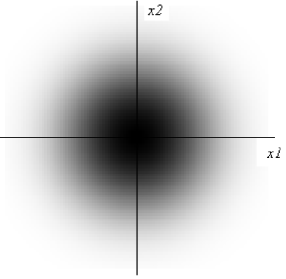
Figure 2: Droplet configuration in the high temperature limit.

The auxiliary function $z$ can be computed in this regime as

$$z^{T}_{B}(R,y) = \frac{1}{2}+\int_{0}^{\infty}n_{B}(R^{\prime})\frac{\partial}{\partial R^{\prime}}z_{0}(R,y;R^{\prime})dR^{\prime}$$ (155)

where

$$n_{B}(R)=N\beta e^{-\beta{R^{2}\over 2}}$$ (156)

and $\beta=1/T$. Making the change of variable $R^{\prime 2}/2=\epsilon$ and using the explicit expression for $z_{0}(R,y;R^{\prime})$ we can write the integral as

$$z^{T}_{B}(R,y)={1\over 2}-2y^{2}N\beta\,I_{z}(\beta,R,y)$$ (157)

where we have defined

$$I_{z}(\beta,R,y)\equiv\int_{0}^{\infty}d\epsilon\;e^{-\beta\epsilon}{(2\epsilon+y^{2}+R^{2})\over[(2\epsilon+y^{2}+R^{2})^{2}-8R^{2}\epsilon]^{3/2}}.$$ (158)

The high temperature limit corresponds to the small $\beta$ region. Therefore we want to find an approximate expression for $I_{z}(\beta,R,y)$ near $\beta=0$. It is easy to verify that $I_{z}(0,R,y)={1\over 2y^{2}}$, and also that

$${\partial I_{z}\over\partial\beta}=-\int_{0}^{\infty}d\epsilon\;{\epsilon\;e^{-\beta\epsilon}(2\epsilon+R^{2}+y^{2})\over[(2\epsilon+y^{2}+R^{2})^{2}-8R^{2}\epsilon]^{3/2}}$$ (159)

diverges as $\ln\beta$ in proximity of $\beta=0$, because the integrand goes like $e^{-\beta\epsilon}/\epsilon$ for large $\epsilon$. This suggests a low $\beta$ expansion of the form

$$I_{z}(\beta,R,y) = I_{z}(0,R,y)+A\beta\ln\beta+...$$

$$z^{T}_{B}(R,y) = {1\over 2}-2y^{2}N\beta\left({1\over 2y^{2}}+A\beta\ln\beta+...\right).$$ (160)

Since it is not possible to compute explicitly ${\partial I_{z}\over\partial\beta}$ for $\beta\rightarrow 0$ because of the divergence, to find its small $\beta$ behavior we find it useful to first regulate the integral by considering the quantity

$${\partial I_{z}\over\partial\beta}+{1\over 4}\int_{0}^{\infty}d\epsilon\;{\epsilon\,e^{-\beta\epsilon}\over\epsilon^{2}+(R^{2}+y^{2})^{2}}.$$ (161)

The new piece

$$I_{0}\equiv-{1\over 4}\int_{0}^{\infty}d\epsilon\;{\epsilon\,e^{-\beta\epsilon}\over\epsilon^{2}+(R^{2}+y^{2})^{2}}$$ (162)

has the same divergence structure of ${\partial I_{z}\over\partial\beta}$ and its value is known for finite $\beta$ in terms of the Sine and Cosine Integral functions $Si(x)$, $Ci(x)$. The corresponding small $\beta$ expansion can be given explicitely as

$$I_{0}=\,{\gamma\over 4}+{1\over 4}\ln[\beta(R^{2}+y^{2})]-{\pi\over 8}\beta(R^{2}+y^{2})+{\cal O}(\beta^{2}\ln\beta)$$ (163)

where $\gamma$ is the Euler-Mascheroni constant. The combination (161) is by construction convergent for any $\beta$, and has a well defined $\beta\rightarrow 0$ limit which can be easily computed analytically

$$\left({\partial I_{z}\over\partial\beta}-I_{0}\right)\Big{|}_{\beta=0}={1\over 4}\left(1-{R^{2}\over y^{2}}\right)-{\ln 2\over 4}+{1\over 4}\ln y^{2}-{1\over 4}\ln(R^{2}+y^{2}).$$ (164)

Using eq. (163) we obtain the high temperature expansion of ${\partial I_{z}\over\partial\beta}$

$${\partial I_{z}\over\partial\beta}={1\over 4}\ln\beta+{1\over 4}\left(\gamma-\ln 2+1-{R^{2}\over y^{2}}+\ln y^{2}\right)+{\cal O}(\beta\ln\beta)$$ (165)

and integrating in $\beta$ we can finally get

$$I_{z}(\beta,R,y)={1\over 2y^{2}}+{1\over 4}\beta\ln\beta+{\beta\over 4}\left(\gamma-\ln 2-{R^{2}\over y^{2}}+\ln y^{2}\right)+{\cal O}(\beta^{2}\ln\beta).$$ (166)

The corresponding high temperature limit of $z^{T}_{B}$, keeping only the first two orders, reads then as follows

$$z^{T}_{B}(R,y)={1\over 2}-N\beta-{Ny^{2}\over 2}\beta^{2}\ln\beta+{\cal O}(\beta^{2}).$$ (167)

To obtain the metric we need to find also the function $V^{T}(R,y)$. Starting from eq. (19) and inserting the Boltzmann distribution we arrive at

$$V^{T}_{B}(R,y)=\int_{0}^{\infty}d\epsilon\;N\beta e^{-\beta\epsilon}{2R^{2}(2\epsilon+y^{2}+R^{2})\over[(2\epsilon+y^{2}+R^{2})^{2}-8R^{2}\epsilon]^{3/2}}\equiv 2N\beta R^{2}I_{V}(\beta,R,y).$$ (168)

One can verify that $I_{V}(0,R,y)$ vanishes and that ${\partial I_{V}\over\partial\beta}$ diverges logarithmically in the $\beta\rightarrow 0$ limit. We can proceed similarly as before by regulating ${\partial I_{V}\over\partial\beta}$ with an appropriate “reference” integral, to finally obtain

$${I_{V}(\beta,R,y)}=-{1\over 4}\beta\ln\beta-{\beta\over 4}\left(\gamma-\ln 2+1+\ln y^{2}\right)+{\cal O}(\beta^{2}\ln\beta).$$ (169)

In proximity of $\beta=0$ the leading contribution to $V^{T}_{B}$ is therefore

$$V^{T}_{B}(R,y)=-{1\over 2}NR^{2}\beta^{2}\ln\beta+{\cal O}(\beta^{2}).$$ (170)

The expressions for $z^{T}_{B}$ and $V^{T}_{B}$ consistently satisfy eq. (17). Note that $z^{T}_{B}$ does not depend on $R$ and that similarly $V^{T}_{B}$ does not depend on $y$. This fact is nevertheless an artefact of the approximation we made. To study its limits of validity, we can look at (167) and (170) and require that the corrections are small: From this we can infer the conditions

$$y^{2}\ll{1\over\beta\ln\beta}\,,\,\,\,\,\,\,\,~{}~{}~{}~{}~{}~{}~{}R^{2}\ll{1\over N\beta^{2}\ln\beta}.$$ (171)

We can now find the metric at first order in the low $\beta$ expansion, i.e. $z^{T}_{B}=1/2-N\beta$ and $V^{T}_{B}=0$. The metric in the LLM coordinates is quickly computed and reads

$$ds^{2}={y\over\sqrt{N\beta}}\left(-dt^{2}+d\Omega_{3}^{2}\right)+{\sqrt{N\beta}\over y}\left(dy^{2}+y^{2}d\tilde{\Omega}_{3}^{2}+dR^{2}+R^{2}d\phi^{2}\right).$$ (172)

Rescaling the coordinates as

$$\tilde{t}=(N\beta)^{-1/4}t,\qquad\tilde{y}=(N\beta)^{1/4}y,\qquad\tilde{R}=(N\beta)^{1/4}R$$ (173)

brings the metric into the form

$$ds^{2}=(N\beta)^{1/4}\tilde{y}\left(-d\tilde{t}^{2}+{1\over\sqrt{N\beta}}d\Omega_{3}^{2}\right)+{1\over(N\beta)^{1/4}\tilde{y}}\left(d\tilde{y}^{2}+\tilde{y}^{2}d\tilde{\Omega}_{3}^{2}+d\tilde{R}^{2}+\tilde{R}^{2}d\phi^{2}\right).$$ (174)

This form of the metric closely resembles the dilute gas approximation limit studied in [7]. There, one considers a configuration of droplets with area $A_{i}$ in the $(x_{1},x_{2})$ plane, and send the distance between the droplets to infinity by the rescaling

$$x\rightarrow\lambda\tilde{x},\qquad x^{\prime}\rightarrow\lambda\tilde{x},\qquad y\rightarrow\lambda\tilde{y},\qquad\lambda\rightarrow\infty$$ (175)

while keeping the droplets areas $A_{i}$ fixed. The corresponding metric reads

$$ds^{2}=H^{-1/2}\left[-d\tilde{t}^{2}+\lambda^{2}d\Omega_{3}^{2}\right]+H^{1/2}\left[d\tilde{y}^{2}+\tilde{y}^{2}d\tilde{\Omega}^{2}_{3}+dx^{i}dx^{i}\right]$$ (176)

where the harmonic function $H$ is

$$H={1\over\pi}\sum_{i}{A_{i}\over[(\tilde{x}-\tilde{x}_{i}^{{}^{\prime}})^{2}+\tilde{y}^{2}]^{2}}.$$ (177)

Thus the metric eq. (176) can be viewed as a multi-center solution for a stack of separated $D3$-branes, and corresponds to the $SO(4)$ invariant sector of the Coulomb branch of the gauge theory.

Upon the identification $\lambda=(N\beta)^{-1/4}$, one can see that the dilute gas limit $\lambda\rightarrow\infty$ is similar to the high temperature regime $\beta\rightarrow 0$ of the thermal solution eq. (174). This is perhaps not surprising since in the high temperature limit the fermion density goes to zero. We also notice that a continuum version of eq. (177) with $A_{i}\equiv d^{2}\tilde{x}^{\prime}/\sqrt{N\beta}$ gives

$$H={1\over\pi}\int{d^{2}\tilde{x}^{\prime}\over\sqrt{N\beta}}\,{1\over[(\tilde{x}-\tilde{x}^{\prime})^{2}+\tilde{y}^{2}]^{2}}={1\over\sqrt{N\beta}\,\tilde{y}^{2}}$$ (178)

which is what we would expect in order to match eq. (174) with eq. (176).

Taking into account the next to leading order corrections for $z^{T}_{B}$ and $V^{T}_{B}$ in eq. (167) and (170), we obtain the metric

$$ds^{2} = H^{-1/2}\left[-dt^{2}+(1-N\beta)d\tilde{\Omega}_{3}^{2}\right]+H^{1/2}\left[dy^{2}+(1+N\beta)y^{2}d\Omega^{2}_{3}+dR^{2}+R^{2}d\phi^{2}\right]$$ (179)

$$+\sqrt{N}R^{2}y\beta^{3/2}\ln\beta dtd\phi$$

where

$$H={N\beta\over y^{2}}-{N^{2}\beta^{2}\over y^{2}}+{1\over 2}\beta^{2}N\ln\beta.$$ (180)

At this order we have a non vanishing $V^{T}_{B}$ and this determines the presence of the mixed term $g_{\phi t}$ in the metric.

5.1 Energy and angular momentum

We remark that the region of validity of the approximations made so far does not allow us to use the metrics (172) and (179) in the asymptotic region $R^{2}+y^{2}\gg 1$, because of the conditions eq. (171). Therefore, to compute the energy of the hyperstar in the high temperature regime, we need to find the form of the metric in the complementary region of validity. The new metric will be trustable in the asymptotic region and will allow a calculation of the energy with the methods already discussed. To this end, it is convenient to first introduce polar coordinates in the $(x_{1},x_{2},y)$ space

$$R = u\cos\vartheta$$ (181)

$$y = u\sin\vartheta.$$ (182)

Then one can evaluate eq. (157) and eq. (168) in an expansion for $u\gg 1$ while keeping $T$ fixed but large (such that we are in the Boltzmann regime). The integrals involved in the expansion can be readily computed analytically and one ends up with the result

$$z^{T}_{B}(u,\vartheta) = {1\over 2}-2N\sin^{2}\vartheta{1\over u^{2}}-8\,NT\sin^{2}\vartheta(3\cos^{2}\vartheta-1){1\over u^{4}}$$ (184)

$$-48\,NT^{2}\sin^{2}\vartheta(10\cos^{4}\vartheta-8\cos^{2}\vartheta+1){1\over u^{6}}+{\cal O}\left({1\over u^{8}}\right)$$

$$V^{T}_{B}(u,\vartheta) = 2N\cos^{2}\vartheta{1\over u^{2}}+8\,NT\cos^{2}\vartheta(3\cos^{2}\vartheta-2){1\over u^{4}}$$ (186)

$$+48\,NT^{2}\cos^{2}\vartheta(10\cos^{4}\vartheta-12\cos^{2}\vartheta+3){1\over u^{6}}+{\cal O}\left({1\over u^{8}}\right)$$

where in the expansion we have kept only terms which contribute to the mass and angular momentum. One can now go to the $AdS_{5}\times S^{5}$ coordinates via the change of variables given in eq. (51) and use $z^{T}_{B}$ and $V^{T}_{B}$ to obtain the asymptotic form of the metric. The explicit expressions are somewhat lengthy and we will not report them here in detail. The computation of $M$ and $J$ follows the same lines of the one given in detail for the low temperature regime. Particularly straightforward is the evaluation of the angular momentum, which can be read off from the shift vector ${\cal N}^{\tilde{\phi}}$. The explicit calculation gives

$${\cal N}^{\tilde{\phi}} = \left({4T\over L^{3}}-L\right){1\over r^{2}}+{\cal O}\left({1\over r^{4}}\right)$$ (187)

$$= {2L\over N^{2}r^{2}}\left(NT-{N^{2}\over 2}\right)+{\cal O}\left({1\over r^{4}}\right)$$ (188)

where we have used the relation $N=L^{4}/2$ which holds in our units. Viewing ${\cal N}^{\tilde{\phi}}dt\equiv A$ as a gauge field in 5 dimensions, the angular momentum is equal to the corresponding electric charge, as explained in the previous section. The result is then

$$J=NT-{N^{2}\over 2}.$$ (189)

This is indeed what we would have expected, since $NT$ is the energy for a gas of $N$ particles with Boltzmann density and $N^{2}/2$ is the ground state energy of the $N$ fermions.

To compute the mass, we used both methods described in sec. 4. Once again, quadratic terms in the charge $(NT-N^{2}/2)$ appear in the calculation, with different coefficients in the two methods. The linear term is however scheme independent and gives the correct result

$$M=\left(NT-{N^{2}\over 2}\right)/L.$$ (190)

6 Conclusion and open questions

In this paper we explored the thermodynamic properties of a 1/2 BPS IIB supergravity solution called hyperstar. This background was first obtained in [9] by thermal coarse-graining of the “bubbling AdS geometry” found in [7]. The hyperstar is in correspondence with a distribution of free fermions in thermodynamic equilibrium at temperature $T$, living on a two-dimensional phase space contained in the ten-dimensional geometry.

We studied both limits of low and high temperature. In the former case, the fermions obey the Fermi-Dirac distribution and the supergravity background is obtained from the LLM Ansatz by means of a Sommerfeld expansion. We found agreement between the energy of the fermions and the ADM mass of the supergravity, modulo a subtlety involving $T^{4}$ terms which we discussed in the main text. We also proposed a way to match the entropy of the fermions with the entropy of the hyperstar in the low temperature limit. String $\alpha^{\prime}$ corrections are expected to generate a finite area stretched horizon, lifting the naked singularity of the hyperstar to a true black hole singularity.

In the classical limit of high temperature, we found the explicit form of the metric of the supergravity background and we observed how this metric resembles the metric of a dilute gas of D3 branes, which corresponds to the $SO(4)$ invariant sector of the Coulomb branch of the CFT. We also computed the associated mass and angular momentum.

It would be interesting to push this study further. An important point, as already remarked, would be to understand better the meaning of the temperature for the supergravity solution. On a more fundamental level, it is worthwile to understand the exact relation between a thermalized solution like the hyperstar and the Matrix Model description of the half-BPS sector of the dual CFT, extending considerations already made in [10].

Another issue is whether the appearance of the naked singularity in the hyperstar can be understood in terms of a distribution of giant gravitons, as is the case for the superstar [15].

The LLM geometries, upon dimensional reduction to five dimension, can be seen as interesting generalizations of AdS half-BPS extremal black holes [30]. It would then be interesting to obtain the explicit dimensional reduction to five dimension of the hyperstar. In this setting one could use the powerful methods of holographic renormalization to carry out the computation of the ADM mass. Then one could prove in a rigorous way that the quadratic contributions to the mass are effectively spurious and can be eliminated within an appropriate renormalization scheme.

Finally, we would like to mention that the LLM construction has been extended to other BPS sectors of type IIB supergravity, see, for instance, [31] for the 1/4 BPS sector. In this case, one modifies the LLM Ansatz in order to accomodate an axion-dilaton field which breaks the supersymmetry by half. The effect of this field is to introduce a deficit angle in the “phase space”. One could try to understand whether this phase space can be useful to study the mass and entropy of the corresponding supergravity geometry.

Acknowledgments

It is a pleasure to thank Gary Gibbons and Martin Roček for discussions and Steven Gubser, Gary Horowitz, Hong Lu, Oleg Lunin and Simon Ross for helpful correspondence. We acknowledge partial financial support through NSF award PHY-0354776.

References

• [1] J. M. Maldacena, “The large N limit of superconformal field theories and supergravity,” Adv. Theor. Math. Phys.  2, 231 (1998) [Int. J. Theor. Phys.  38, 1113 (1999)] [arXiv:hep-th/9711200]; E. Witten, “Anti-de Sitter space and holography,” Adv. Theor. Math. Phys.  2, 253 (1998) [arXiv:hep-th/9802150].
• [2] D. Berenstein, “A toy model for the AdS/CFT correspondence,” JHEP 0407, 018 (2004) [arXiv:hep-th/0403110].
• [3] V. Balasubramanian, M. Berkooz, A. Naqvi and M. J. Strassler, “Giant gravitons in conformal field theory,” JHEP 0204, 034 (2002) [arXiv:hep-th/0107119]; S. Corley, A. Jevicki and S. Ramgoolam, “Exact correlators of giant gravitons from dual N = 4 SYM theory,” Adv. Theor. Math. Phys.  5, 809 (2002) [arXiv:hep-th/0111222].
• [4] I. R. Klebanov, “String theory in two-dimensions,” arXiv:hep-th/9108019.
• [5] J. McGreevy and H. L. Verlinde, “Strings from tachyons: The c = 1 matrix reloaded,” JHEP 0312, 054 (2003) [arXiv:hep-th/0304224].
• [6] Y. Nakayama, “Liouville field theory: A decade after the revolution,” Int. J. Mod. Phys. A 19, 2771 (2004) [arXiv:hep-th/0402009].
• [7] H. Lin, O. Lunin and J. Maldacena, “Bubbling AdS space and 1/2 BPS geometries,” JHEP 0410, 025 (2004) [arXiv:hep-th/0409174].
• [8] D. Martelli and J. F. Morales, “Bubbling AdS(3),” JHEP 0502, 048 (2005) [arXiv:hep-th/0412136]; J. T. Liu and D. Vaman, “Bubbling 1/2 BPS solutions of minimal six-dimensional supergravity,” arXiv:hep-th/0412242; H. Ebrahim and A. E. Mosaffa, “Semiclassical string solutions on 1/2 BPS geometries,” JHEP 0501, 050 (2005) [arXiv:hep-th/0501072]; G. Mandal, “Fermions from half-BPS supergravity,” JHEP 0508, 052 (2005) [arXiv:hep-th/0502104]; P. Horava and P. G. Shepard, “Topology changing transitions in bubbling geometries,” JHEP 0502, 063 (2005) [arXiv:hep-th/0502127]; Y. Takayama and K. Yoshida, “Bubbling 1/2 BPS geometries and Penrose limits,” Phys. Rev. D 72, 066014 (2005) [arXiv:hep-th/0503057]; L. Grant, L. Maoz, J. Marsano, K. Papadodimas and V. S. Rychkov, “Minisuperspace quantization of ’bubbling AdS’ and free fermion droplets,” JHEP 0508, 025 (2005) [arXiv:hep-th/0505079]; A. Ghodsi, A. E. Mosaffa, O. Saremi and M. M. Sheikh-Jabbari, “LLL vs. LLM: Half BPS sector of N = 4 SYM equals to quantum Hall system,” Nucl. Phys. B 729, 467 (2005) [arXiv:hep-th/0505129]; I. Bena and N. P. Warner, “Bubbling supertubes and foaming black holes,” arXiv:hep-th/0505166; S. Mukhi and M. Smedback, “Bubbling orientifolds,” JHEP 0508, 005 (2005) [arXiv:hep-th/0506059]; M. Boni and P. J. Silva, “Revisiting the D1/D5 system or bubbling in AdS(3),” JHEP 0510, 070 (2005) [arXiv:hep-th/0506085]; Y. Takayama and A. Tsuchiya, “Complex matrix model and fermion phase space for bubbling AdS geometries,” JHEP 0510, 004 (2005) [arXiv:hep-th/0507070]; L. Maoz and V. S. Rychkov, “Geometry quantization from supergravity: The case of ’bubbling AdS’,” JHEP 0508, 096 (2005) [arXiv:hep-th/0508059]; P. J. Silva, “Rational foundation of GR in terms of statistical mechanic in the AdS/CFT framework,” JHEP 0511, 012 (2005) [arXiv:hep-th/0508081]; J. Dai, X. J. Wang and Y. S. Wu, “Dynamics of giant-gravitons in the LLM geometry and the fractional quantum Hall effect,” Nucl. Phys. B 731, 285 (2005) [arXiv:hep-th/0508177]; M. Alishahiha, H. Ebrahim, B. Safarzadeh and M. M. Sheikh-Jabbari, “Semi-classical probe strings on giant gravitons backgrounds,” JHEP 0511, 005 (2005) [arXiv:hep-th/0509160]; H. Lin and J. Maldacena, “Fivebranes from gauge theory,” arXiv:hep-th/0509235.
• [9] A. Buchel, “Coarse-graining 1/2 BPS geometries of type IIB supergravity,” arXiv:hep-th/0409271.
• [10] V. Balasubramanian, J. de Boer, V. Jejjala and J. Simon, “The library of Babel: On the origin of gravitational thermodynamics,” arXiv:hep-th/0508023.
• [11] M. M. Caldarelli, D. Klemm and P. J. Silva, “Chronology protection in anti-de Sitter,” Class. Quant. Grav.  22, 3461 (2005) [arXiv:hep-th/0411203].
• [12] G. Milanesi and M. O Loughlin “Singularities and closed time-Like curves in Type IIB $1/2$ BPS Geometries” JHEP 0509, 008 (2005) [arXiv:hep-th/0507056].
• [13] A. Dabholkar, “Exact counting of black hole microstates,” Phys. Rev. Lett.  94, 241301 (2005) [arXiv:hep-th/0409148]; A. Dabholkar, R. Kallosh and A. Maloney, “A stringy cloak for a classical singularity,” JHEP 0412, 059 (2004) [arXiv:hep-th/0410076].
• [14] O. Lunin and S. D. Mathur, “Statistical interpretation of Bekenstein entropy for systems with a Phys. Rev. Lett.  88, 211303 (2002) [arXiv:hep-th/0202072].
• [15] R. C. Myers and O. Tafjord, “Superstars and giant gravitons,” JHEP 0111, 009 (2001) [arXiv:hep-th/0109127].
• [16] N. V. Suryanarayana, “Half-BPS giants, free fermions and microstates of superstars,” arXiv:hep-th/0411145.
• [17] P. G. Shepard, “Black hole statistics from holography,” JHEP 0510, 072 (2005) [arXiv:hep-th/0507260].
• [18] L. D. Landau and E. M.  Lifshitz, “Statistical Physics: Part 1”, Pergamon Press, (1969).
• [19] J. D. Brown and J. W. York, “Quasilocal energy and conserved charges derived from the gravitational action,” Phys. Rev. D 47, 1407 (1993).
• [20] V. Balasubramanian and P. Kraus, “A stress tensor for anti-de Sitter gravity,” Commun. Math. Phys.  208, 413 (1999) [arXiv:hep-th/9902121].
• [21] K. Skenderis, “Lecture notes on holographic renormalization,” Class. Quant. Grav.  19, 5849 (2002) [arXiv:hep-th/0209067].
• [22] M. Taylor-Robinson, “Higher-dimensional formulation of counterterms,” arXiv:hep-th/0110142.
• [23] R. C. Myers, “Stress tensors and Casimir energies in the AdS/CFT correspondence,” Phys. Rev. D 60, 046002 (1999) [arXiv:hep-th/9903203].
• [24] S. W. Hawking and G. T. Horowitz, “The Gravitational Hamiltonian, action, entropy and surface terms,” Class. Quant. Grav.  13, 1487 (1996) [arXiv:gr-qc/9501014].
• [25] K. Behrndt, M. Cvetic and W. A. Sabra, “Non-extreme black holes of five dimensional N = 2 AdS supergravity,” Nucl. Phys. B 553, 317 (1999) [arXiv:hep-th/9810227].
• [26] M. Cvetic et al., “Embedding AdS black holes in ten and eleven dimensions,” Nucl. Phys. B 558, 96 (1999) [arXiv:hep-th/9903214].
• [27] A. Buchel and L. A. Pando Zayas, “Hagedorn vs. Hawking-Page transition in string theory,” Phys. Rev. D 68, 066012 (2003) [arXiv:hep-th/0305179].
• [28] J. T. Liu and W. A. Sabra, “Mass in anti-de Sitter spaces,” Phys. Rev. D 72, 064021 (2005) [arXiv:hep-th/0405171].
• [29] M. M. Caldarelli and P. J. Silva, “Giant gravitons in AdS/CFT. I: Matrix model and back reaction,” JHEP 0408, 029 (2004) [arXiv:hep-th/0406096].
• [30] Z. W. Chong, H. Lu and C. N. Pope, “BPS geometries and AdS bubbles,” Phys. Lett. B 614, 96 (2005) [arXiv:hep-th/0412221].
• [31] J. T. Liu, D. Vaman and W. Y. Wen, “Bubbling 1/4 BPS solutions in type IIB and supergravity reductions on S**n x S**n,” arXiv:hep-th/0412043.