Resonances in the one-dimensional Dirac equation in the presence of a point interaction and a constant electric field

Abstract

We show that the energy spectrum of the one-dimensional Dirac equation in the presence of a spatial confining point interaction exhibits a resonant behavior when one includes a weak electric field. After solving the Dirac equation in terms of parabolic cylinder functions and showing explicitly how the resonant behavior depends on the sign and strength of the electric field, we derive an approximate expression for the value of the resonance energy in terms of the electric field and delta interaction strength.

,

1 Introduction

Supercritical effects are perhaps one of the most interesting phenomena associated with the charged vacuum in the presence of strong electric fields [1, 2] The study of supercritical effects induced by strong vector potentials goes back to the pioneering works of Pieper and Greiner [3], Zeldovich and Popov [4] among others. The idea behind supercriticality is to have positron emission induced by the presence of very strong attractive vector potentials. The phenomenon can be described as follows: the energy level of an unoccupied bound state dives into the negative energy continuum. i.e., an electron of the Dirac sea is trapped by the potential, leaving a positron that escapes to infinity.  The electric field responsible for supercriticality should be stronger than $2m_{e}c^{2}$, which is the value of the gap between the negative and positive energy continua.  Such strong electric fields could be produced in heavy-ion collisions [1, 5]. A rigorous mathematical study of the behavior of the Dirac energy levels near the continuum spectrum and the problem of spontaneous pair creation has been carried out by S̆eba [6], Klaus [7] and Nenciu [8] among others.

In order to get a deeper understanding of the mechanism responsible for supercriticality and for the resonant peaks appearing in the energy spectrum when supercritical fields are present, we proceed to work with a vector point interaction in the presence of a constant electric field. Point interactions potentials may be used to approximate, in a simple way, more complex short-ranged potentials. Among the advantages of working with confining delta interactions we should mention that, they only possess a single bound state and the treatment of the interacting potential reduces to a boundary condition. The study of bound states of the relativistic wave equation in the presence of point interactions is a problem that has been carefully discussed in the literature [9, 10, 11, 12, 13]. The one-dimensional Dirac equation in the presence of a vector point delta interaction has also been a subject of study in the search of supercritical effects induced by attractive potentials [1, 14]. Soon after the publication of the paper by Loewe and Sanhueza [14], Nogami et al [15] pointed out that supercritical effects are also absent in a class of non-local separable potentials in one dimension.

Since we are interested in studying the mechanism of positron production by supercritical fields, we proceed to analyze the resonant behavior of the energy when a bound state dives into the negative continuum. This resonant behavior is associated with the appearance of simple poles of the resolvent on the second sheet at a position very near the real axis [16].

The method of complex eigenvalues (Gamow vectors) was introduced in quantum mechanics by Gamow [17] in connection with the theory of Alpha decay. Titchmarsch [18] and Barut [19] demonstrated an application, in the framework of non-relativistic quantum mechanics, for the Gamow vector method to the problem of an attractive delta interaction $\delta(r)$ of strength $-\cot\alpha$ with a weak electric field term associated with the potential $V(r)=-\lambda r.$ They found that the Schrödinger equation with a weak electric field exhibits a continuous spectrum from $-\infty$ to $+\infty,$ and a resonance at $E^{{}^{\prime}}$ in the vicinity of $E_{{0}}-\frac{1}{2}\lambda\tan\alpha,$ where $E_{0}=-\cot^{2}\alpha$ is the energy of the unperturbed state. The eigenvalue $E^{{}^{\prime}}$ is a complex number in the lower half plane.  According to Barut, the Schrödinger equation with the potential $-\lambda r$ describes a system that tries to form a bound state that “dissolves itself” in the presence of the continuous spectrum. In this Letter, using  the idea developed by Titchmarsch [18], we find the energy spectrum of the one-dimensional Dirac equation with boundary conditions associated with a vector Dirac delta interaction and a constant electric field whose strength is weak, and therefore it produces a perturbative effect on the delta energy spectrum. We find that in this case the energy spectrum exhibits a resonance due to supercriticality.

The Letter is structured as follows: In Section 2, we solve the one-dimensional Dirac equation in the presence of an attractive $\delta$ potential and a constant electric field. In Section 3, we compute the energy resonances and show how they depend on the electric field strength. We also derive an approximate analytic expression for the energy resonances. Finally, in Section 4 we summarize our conclusions.

2 The one-dimensional Dirac equation

In this section we will consider the 1+1 Dirac equation in the presence of the attractive vector point interaction potential represented by $eV(x)=-g_{v}\delta(x),$ and a constant electric field associated with the potential $eV(x)=\lambda x$.  The Dirac equation, expressed in natural units ($\hslash=c=1$) can be written in the form [20]

$$\left(i\gamma^{\mu}(\frac{\partial}{\partial x^{\mu}}-ieA_{\mu})-m\right)\Psi=0,$$ (1)

where $A_{\mu}$ is the vector potential, $e$ is the charge and $m$ is the mass of the electron. The Dirac matrices $\gamma^{\mu}$ satisfy the commutation relation $\left\{\gamma^{\mu},\gamma^{\nu}\right\}=2\eta^{\mu\nu}$ with $\eta^{\mu\nu}=\mathrm{diag}(1,-1).$ Since we are working in 1+1 dimensions, we choose to work in a two-dimensional representation of the  Dirac matrices

$$\gamma^{0}=\sigma_{3},\gamma^{1}=-i\sigma_{2}.$$ (2)

Substituting the representation matrix representation (2) into Eq. (1), and taking into account that the potential interaction does not depend on time, we obtain

$$\{-i\sigma_{{1}}\frac{d}{dx}+\left(\lambda x-E\right)+m\sigma_{{3}}\}\mathsf{X}(x)=0,$$ (3)

with $\Psi=\sigma_{3}\mathsf{X.}$, and

$$\mathsf{X}(x)=\begin{pmatrix}X_{{1}}\\ X_{{2}}\end{pmatrix},$$ (4)

with the boundary conditions at $x=0$

$$\begin{split}X_{{1}}(0^{{+}})&=X_{{1}}(0^{{-}})\cos{g_{{v}}}-iX_{{2}}(0^{{-}})\hskip 2.84544pt\mathrm{\sin}{g_{{v}}},\\ X_{{2}}(0^{{+}})&=-iX_{{1}}(0^{{-}})\hskip 2.84544pt\mathrm{\sin}{g_{{v}}}+X_{{2}}(0^{{-}})\cos{g_{{v}}}.\end{split}$$ (5)

The above conditions (5) describe a the point vector potential interaction of strength $g_{{v}}$ [12].

Equation (3) is equivalent to the system of equations

$$\left(m+\lambda x-E\right)X_{{1}}-i\frac{dX_{2}}{dx}=0,$$ (6)

$$i\frac{dX_{1}}{dx}+\left(m-\lambda x+E\right)X_{{2}}=0,$$ (7)

Introducing the new functions $\Omega_{{1}}$ and $\Omega_{{2}}$

$$X_{{1}}=\Omega_{{1}}+i\Omega_{{2}},\quad X_{{2}}=\Omega_{{1}}-i\Omega_{{2}},$$ (8)

we obtain that the system of equations (6) -(7) reduces to the form

$$\frac{d\Omega_{1}}{dx}+i\left(\lambda x-E\right)\Omega_{{1}}-m\Omega_{{2}} =0,$$ (9)

$$\frac{d\Omega_{{2}}}{dx}-i\left(\lambda x-E\right)\Omega_{{2}}-m\Omega_{{1}} =0,$$ (10)

which is more tractable in the search of exact solutions. Substituting (9) into (10) we obtain the second-order differential equation

$$\frac{d^{2}\Omega_{{1}}}{dx^{2}}\,+\{i\lambda+\left(\lambda x-E\right)^{2}-m^{2}\}\,\Omega_{{1}}=0.$$ (11)

Looking at the asymptotic behavior of the parabolic cylinder functions $D_{\nu}(z)$ [21] we obtain that the regular solutions, for $\lambda>0$, of Eq. (11) belonging to $\mathcal{L}^{2}(-\infty,0)$ and $\mathcal{L}^{2}(0,\infty)$ ($Im\,E>0$), respectively are

$$\begin{split}\Omega_{{1}}^{-}(x)&=AD_{{-\rho-1}}\left(\sqrt{\frac{2}{\lambda}}e^{{-i\frac{\pi}{4}}}\left(\lambda\,x-E\right)\right)\\ \Omega_{1}^{+}(x)&=BD_{\rho}\left(\sqrt{\frac{2}{\lambda}}e^{{i\frac{\pi}{4}}}\left(\lambda\,x-E\right)\right),\end{split}$$ (12)

where $D_{{\rho}}$ y $D_{{-\rho-1}}$ are parabolic cylinder functions [21], $\rho=\frac{im^{{2}}}{2\lambda}$,  and $A$ and $B$ are constants.

Inserting (12) into (9) and using the recurrence relations for the parabolic cylinder functions [21], we obtain

$$\begin{split}\Omega_{2}^{-}(x)&=i\frac{\sqrt{2\lambda}}{m}e^{{i\frac{\pi}{4}}}AD_{{-\rho}}\left(\sqrt{\frac{2}{\lambda}}e^{{-i\frac{\pi}{4}}}\left(\lambda\,x-E\right)\right),\\ \Omega_{2}^{+}(x)&=i\frac{m}{\sqrt{2\lambda}}e^{{i\frac{\pi}{4}}}BD_{{\rho-1}}\left(\sqrt{\frac{2}{\lambda}}e^{{i\frac{\pi}{4}}}\left(\lambda\,x-E\right)\right).\end{split}$$ (13)

From (12), (13) and (8), we have that the components of the spinor solution for $x<0$ are

$$\begin{split}X_{1}^{-}(x)&=A\left[D_{{-\rho-1}}\left(\sqrt{\frac{2}{\lambda}}e^{{-i\frac{\pi}{4}}}\left(\lambda\,x-E\right)\right)-\frac{\sqrt{2\lambda}}{m}e^{{i\frac{\pi}{4}}}D_{{-\rho}}\left(\sqrt{\frac{2}{\lambda}}e^{{-i\frac{\pi}{4}}}\left(\lambda\,x-E\right)\right)\right],\\ X_{{2}}^{-}(x)&=A\left[D_{{-\rho-1}}\left(\sqrt{\frac{2}{\lambda}}e^{{-i\frac{\pi}{4}}}\left(\lambda\,x-E\right)\right)+\frac{\sqrt{2\lambda}}{m}e^{{i\frac{\pi}{4}}}D_{{-\rho}}\left(\sqrt{\frac{2}{\lambda}}e^{{-i\frac{\pi}{4}}}\left(\lambda\,x-E\right)\right)\right],\end{split}$$ (14)

analogously, we have that, for $x>0$, the spinor $\mathsf{X}$ has the components:

$$\begin{split}X_{{1}}^{+}(x)&=B\left[D_{{\rho}}\left(\sqrt{\frac{2}{\lambda}}e^{{i\frac{\pi}{4}}}\left(\lambda\,x-E\right)\right)-\frac{m}{\sqrt{2\lambda}}e^{{i\frac{\pi}{4}}}D_{{\rho-1}}\left(\sqrt{\frac{2}{\lambda}}e^{{i\frac{\pi}{4}}}\left(\lambda\,x-E\right)\right)\right],\\ X_{{2}}^{+}(x)&=B\left[D_{{\rho}}\left(\sqrt{\frac{2}{\lambda}}e^{{i\frac{\pi}{4}}}\left(\lambda\,x-E\right)\right)+\frac{m}{\sqrt{2\lambda}}e^{{i\frac{\pi}{4}}}D_{{\rho-1}}\left(\sqrt{\frac{2}{\lambda}}e^{{i\frac{\pi}{4}}}\left(\lambda\,x-E\right)\right)\right].\end{split}$$ (15)

Inserting (14) and (15) in (5), we obtain that the equation for the energy eigenvalues $E$ has the form:

$$\begin{split}2\lambda D_{{\rho}}\left(\sqrt{\frac{2}{\lambda}}e^{{i\frac{\pi}{4}}}E\right)&D_{{-\rho}}\left({-\sqrt{\frac{2}{\lambda}}}e^{{-i\frac{\pi}{4}}}E\right)\\ &-m^{{2}}D_{{\rho-1}}\left(\sqrt{\frac{2}{\lambda}}e^{{i\frac{\pi}{4}}}E\right)D_{{-\rho-1}}\left({-\sqrt{\frac{2}{\lambda}}}e^{{-i\frac{\pi}{4}}}E\right)e^{{-2ig_{{v}}}}=0.\end{split}$$ (16)

The regular solutions of Eq. (11), for $\lambda<0$, can be obtained after interchanging the roles of $\Omega_{1}^{-}(x)$ and $\Omega_{1}^{+}(x)$ and of $\Omega_{2}^{-}(x)$ and $\Omega_{2}^{+}(x)$ in Eq. (12) and Eq. (13) respectively; therefore Eq. (16) permits us to compute the energy resonances for positive as well as negative values of the electric field strength $\lambda$

3 Energy resonances

It is not an easy task to solve Eq. (16), nevertheless it is possible to derive an analytic approximation for the energy eigenvalues. In order to do this approximation we consider the effect of the electric field in the vicinity of zero, i.e., where the delta interaction is located. We insert the spinor solutions obtained using this approach into (5), obtaining in this way an eigenvalue equation, whose roots are a good approximation to those of (16). The approximate equation for $\Omega_{{1}}$ has the form

$$\frac{d^{2}\Omega_{{1}}}{dx^{2}}\,+\{i\lambda+E^{2}-m^{2}\}\,\Omega_{{1}}=0.$$ (17)

The solution of Eq. (17) that, for $x>0$, and $\lambda>0$ exhibit a regular asymptotic behavior is

$$\Omega_{1}^{+}=A\exp(-i\sqrt{i\lambda+E^{2}-m^{2}}x).$$ (18)

Substituting the solution (18) into Eq. (9) we obtain

$$\Omega_{2}^{+}=-iA\frac{\sqrt{i\lambda+E^{2}-m^{2}}+E}{m}\exp(-i\sqrt{i\lambda+E^{2}-m^{2}}x),$$ (19)

and, analogously, we have that for $x<0,$ the corresponding solutions are

$$\Omega_{1}^{-}=B\exp(i\sqrt{i\lambda+E^{2}-m^{2}}x),$$ (20)

$$\Omega_{2}^{-}=-iB\frac{-\sqrt{i\lambda+E^{2}-m^{2}}+E}{m}\exp(i\sqrt{i\lambda+E^{2}-m^{2}}x).$$ (21)

Substituting the right $\Omega_{1,2}^{+}$ and left $\Omega_{1,2}^{-}$ spinor components into Eq. (5), we find that, for $g_{v}=-\pi$, the energy state sinks into the negative energy continuum, exhibiting a resonant behavior that depends on the electric field strength as:

$$E\left(\lambda\right)\approx-\left(m+\frac{\lambda^{{2}}}{8m^{{3}}}\right)+i\frac{\lambda}{2m},$$ (22)

where we have assumed that $\lambda$ is positive and small compared to $m$. It should be noticed that, when we turn off the electric perturbation, we recover the energy eigenvalue $E(0)=-m$ for a point vector interaction with strength $g_{{v}}=-\pi$ [12]. It is worth mentioning the vanishing of the first order perturbative correction to the supercritical energy $E=-m$ as a result of the presence of the electric field interaction $\lambda$. This behavior can also be observed looking at the real part of the resonant energy given by Eq. (22). An approximate expression for the energy resonances for negative values of $\lambda$ can be obtained after substituting $\lambda$ by $-\lambda$ in Eq. (22).

We can try to obtain an approximate solution to the full Eq. (11) after making a series expansion of the function $\ i\lambda+\left(\lambda x-E\right)^{2}-m^{2}$ around zero. In this way, we have that the approximate function $\Omega_{{1}}$ satisfies the second order differential equation

$$\frac{d^{2}\Omega_{{1}}}{dx^{2}}\,+\{i\lambda+E^{2}-2\lambda Ex-m^{2}\}\,\Omega_{{1}}=0.$$ (23)

The regular solutions $\Omega_{{1}}^{-}$ and for $x<0,$ and $\Omega_{{1}}^{+}$ for $x>0$ can be expressed, for $\lambda>0$, in terms of Hankel functions $H_{1/3}^{1}(z)$ and $H_{1/3}^{2}(z)$ [22] as follows

$$\Omega_{{1}}^{-}=Az^{1/3}H_{1/3}^{1}(z),$$ (24)

$$\Omega_{{1}}^{+}=Bz^{1/3}H_{1/3}^{2}(z),$$ (25)

where $A$ and $B$ are constants and $z$ is given by the expression

$$z=-\frac{\left(i\lambda+E^{2}-m^{2}-2E\lambda x\right)^{3/2}}{3\lambda E}$$ (26)

Substituting the solutions (24) and (25) for $\Omega_{{1}}^{-}$ and $\Omega_{{1}}^{+}$ into Eq. (9) we obtain the corresponding expressions for $\Omega_{{2}}^{-}$ and $\Omega_{{2}}^{+}.$  Taking into account the relation between $X_{1}$, $X_{2}$ and $\Omega_{1},$ $\Omega_{2}$ (8), and inserting the lower and upper components of $\mathsf{X}$ into the boundary condition (5), we find that an approximate equation for the energy spectrum is:

$$\left(X_{{2}}(0^{{-}})X_{{1}}(0^{{+}})-X_{{2}}(0^{{+}})X_{{1}}(0^{{-}})\right)\cos g_{v}+i\left(X_{{2}}(0^{{+}})X_{{2}}(0^{{+}})-X_{{1}}(0^{{+}})X_{{1}}(0^{{-}})\right)\sin g_{v}=0$$ (27)

It is worth noting that the energy spectrum obtained from Eq. (27) with $\Omega_{{1}}^{-}$ and $\Omega_{{1}}^{+}$ given by Eqs. (24) and (25) gives a result comparable to the one obtained using the relation Eq. (22)

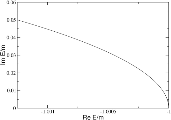
Figure 1: Dependence of the real and imaginary parts of the energy on the electric field strength for $0<\lambda<0.1m^{2}$.

Fig. 1 shows how the real and imaginary part of the energy depend on the parameter $\lambda$ when a point vector interaction of strength $g_{{v}}=-\pi$ is applied. The energy exhibits a resonant behavior produced by the electric field.

The inverse of the imaginary part of Eq. (22) permits one to determine the time [23, 24] that the state stays in negative continuum. The stronger the electric field perturbation, the shorter the mean life of the resonance [23]. An interesting result that can be observed from Eq. (22) and it is also depicted in Fig. 1 is that the imaginary part of the resonant energy behaves as a square root with respect to the real part of the energy.

4 Concluding remarks

In this article we have shown that the presence of a weak electric field plays a crucial role in the appearance of a resonant energy state in the one-dimensional Dirac equation in the field of an attractive vector delta interaction. This phenomenon is analogous to the Stark effect [25], where a perturbative constant electric field produces a shifting and broadening of the energy levels of the hydrogen atom. It also parallels the autoionization process, where the presence electron-electron interaction term induces a self-ionization process and levels decay like in the Auger effect [16, 25]. Such analogies seem to indicate that, for resonant effects, the shape of the perturbative potential is sometimes more important than the strength of the potential field.

We have also shown that, the one-dimensional Dirac equation in the field of an attractive vector delta interaction exhibits a resonant supercritical behavior when one introduces a potential of the form $\lambda x$. Since this effect is not present when one consider the sole vector interaction $-g_{v}\delta(x)$ [12], we conclude that it is necessary the presence of the electric field in order to sink the delta bound state into the negative continuum.

5 Acknowledgments

We thank Dr. Ernesto Medina for reading and improving the manuscript. We also wish to express our gratitude to the anonymous referees for their critical remarks. This work was supported by FONACIT under project G-2001000712.

References

- [1] W. Greiner, B. Müller, and J. Rafelski, Quantum Electrodynamics of Strong fields (Springer Verlag, Berlin, 1985).
- [2] J. Rafelski, P. Fulcher and A. Klein Phys. Rep. 38 (1978) 227.
- [3] W. Pieper, and W. Greiner, Z. Phys. 218, (1969) 327.
- [4] Y. B. Zeldovich, and V. S. Popov, Sov. Phys. Usp. 14 (1972) 673.
- [5] W. Greiner and J. Reinhardt, Physica Scripta T56, (1995) 203.
- [6] P. S̆eba, The Dirac eigenvalues near upper and lower continuum, Preprint JINR E2-86-808, Dubna 1986.
- [7] M. Klaus, J. für Mathematik, 362, 197 (1985).
- [8] G. Nenciu, Commun. Math. Phys. 109 303 (1987).
- [9] B. Sutherland and D. C. Mattis, Phys. Rev. A 24, (1981) 1194.
- [10] B. H. J. McKellar and G. J. Stephenson, Phys. Rev. A. 36 (1987) 2566.
- [11] B. H. J. McKellar and G. J. Stephenson, Phys. Rev. C. 35 (1987) 2262.
- [12] F. Domínguez-Adame and E. Maciá, J. Phys. A: Math. Gen. 22 (1989) L419.
- [13] S. Albeverio, F. Gesztesy, R. Høegh-Krohn and H. Holden, Solvable Models in Quantum Mechanics(AMS Chelsea Publishing, Providence, Rhode Island 2005)
- [14] M. Loewe and M. Sanhueza, J. Phys. A: Math. Gen. 23, (1990) 553.
- [15] Y. Nogami, N. P.Parent and F. M. Tokoyama, J. Phys. A: Math. Gen 23, (1990) 5667.
- [16] M. Reed and B. Simon, Methods of Modern Mathematical Physics: IV Analysis of Operators (Academic Press, New York 1978).
-
[17]
G. Gamow, Z. Phys. 51, (1928) 204.
E.U. Condon, and R. W. Gurney, Phys. Rev. 33, (1929) 127. - [18] E. C. Titchmarsh, Eigenfunction Expansions Associated with Second Order Differential Equations, Part II. (Oxford University Press, Oxford 1958).
- [19] W. E. Brittin, Lectures in Theoretical Physics, Vol. IV. Interscience Publishers, 1962, Pag. 460.
- [20] W. Greiner, Relativistic Quantum Mechanics, Wave equations, (Springer, New York 1990).
- [21] Higher Transcendental Functions, Vol. II. McGraw - Hill Book Company, Inc., 1953.
- [22] M. Abramowitz and I. Stegun, Handbook of Integrals, Series and Products (Dover, New York 1965).
- [23] R. G. Newton, Scattering Theory of Waves and Particles, (Dover, New York, 2002)
- [24] M. Goldberger and K. Watson, Collision Theory (Dover, New York, 2004)
- [25] A. Galindo, and P. Pascual, Quantum Mechanics II (Springer-Verlag, Heidelberg, 1991).