SISSA-71/2005/EP

CERN-PH-TH/2005-224

QMUL-PH-05-10

DFTT-05-34

Brane world effective actions

for D-branes with fluxes

M. Bertolini
SISSA/ISAS and INFN - Sezione di Trieste
Via Beirut 2; I-34014 Trieste, Italy

M. Billò

Dipartimento di Fisica Teorica, Università di Torino
and INFN - Sezione di Torino; Via P. Giuria 1; I-10125 Torino, Italy

A. Lerda

Dipartimento di Scienze e Tecnologie Avanzate, Università del Piemonte Orientale
Via V. Bellini 25/G; I-15100 Alessandria, Italy
and INFN - Sezione di Torino

J.F. Morales and R. Russo

CERN, Physics Department
CH-1211 Geneva 23, Switzerland

Abstract

We develop systematic string techniques to study brane world effective actions for models with magnetized (or equivalently intersecting) D-branes. In particular, we derive the dependence on all NS-NS moduli of the kinetic terms of the chiral matter in a generic non-supersymmetric brane configurations with non-commuting open string fluxes. Near a ${\cal N}=1$ supersymmetric point the effective action is consistent with a Fayet-Iliopoulos supersymmetry breaking and the normalization of the scalar kinetic terms is nothing else than the Kähler metric. We also discuss, from a stringy perspective, $D$ and $F$ term breaking mechanisms, and how, in this generic set up, the Kähler metric enters in the physical Yukawa couplings.

1 Introduction and Summary

In Type II and Type I string theories, D-branes are the objects providing, in a simple and natural way, two important features of our world: the presence of non-abelian gauge groups and that of four dimensional chiral fermions. In particular, when the ten dimensional space-time is simply taken to be the direct product of a six dimensional compact manifold and of a four dimensional Minkowski part, chiral fermions arise when the D-branes have some non-trivial properties in the compact space. This can happen when constant magnetic fields are switched on along the D-brane world-volume [1], or when the D-branes intersect with some non-trivial angles [2] (actually, these two situations can be usually connected by means of some T-dualities, see for instance [3]). By exploiting these basic features, a new class of string models has been studied in these last years, starting from [4, 5, 6], providing various interesting phenomenological applications. Recent reviews on this subject, often named “Intersecting Brane Worlds” (IBW) [7], are Refs. [8, 9, 10, 11, 12] and also the detailed derivation of some results can be found in the PhD-theses [13, 14, 15, 16]. One of the nice features of this class of string models is that they are “calculable”. This means that, by using known string techniques, it is possible to compute explicitly the Standard-Model-like effective action. Moreover, all the parameters appearing in such a low-energy action are functions of the microscopic data specifying the D-brane configuration and the geometry of the compact space. The explicit derivation of the effective action is certainly possible whenever the string vacuum under consideration is described, from the world-sheet point of view, by some tractable Conformal Field Theory (CFT). Even if this is a rather particular set of points in the whole moduli space of the D-brane/string compactifications, it contains already some very interesting situations, like those involving orbifolds or orientifolds and, as we already said, also the case of D-branes with constant magnetic fields. Thanks to the simplicity of the underlying string theory, it has been possible to study various features of the IBW models which go beyond the analysis of the spectrum and of its quantum numbers. For instance, several authors studied how the Higgs mechanism [17] and the Yukawa couplings [18, 19, 20, 21] are realized in intersecting brane models (or in the T-dual case of magnetized D-branes [22]); some of their phenomenological implications are discussed in [23, 24]; threshold corrections [25, 26] have been computed; proton decay can be studied quantitatively [27, 28]; it has also been shown that the problem of moduli stabilization can be partly addressed in the framework of solvable string models, by using D-brane world-volume fluxes [29]. The issue of complete moduli stabilization has been thoroughly studied, see for instance Refs. [30, 31, 32, 33, 34, 35, 36, 37, 38, 39, 40, 41, 26]; however generically these constructions go beyond the class of “solvable” models we consider in this paper. Various recent papers discuss phenomenological features of open string models, where the techniques analyzed in this paper might be useful, see for instance Refs. [42, 43, 44, 45, 46, 47, 48].

In this paper we describe in some generality the string theory techniques necessary to compute the effective actions for this class of string models, where the Standard Model fields live on intersecting or magnetized D-branes. The technique we use is conceptually simple and well-known: one can reconstruct the effective action by requiring that it reproduces the low energy limit of the string amplitudes. Thus this is a two steps procedure: first it is necessary to compute a string amplitude contributing to a particular term of the effective action one is interested in; then one can extract the low-energy amplitude by sending the string length $\sqrt{\alpha^{\prime}}$ to zero with all four dimensional momenta and masses kept fixed. We focus on the dynamics of the fields coming from the open strings and try to determine the dependence of the relevant pieces of the four dimensional effective action on the closed string moduli, whose dynamics is kept frozen (ı.e. we work in a limit where gravity is non dynamical on the brane). This technique has been explicitly applied in Heterotic string theory by Dixon, Louis and Kaplunovsky [49] and more recently in the context of IBW in Ref. [21]. Here we follow the same approach, with the goal to generalize it in various directions. First we show that this technique is not limited to supersymmetric models. On the contrary, it is most effective in situations where supersymmetry is spontaneously broken, because in this cases we can use the presence of mass terms to fix unambiguously the overall normalization of the string amplitudes, which actually plays an important rôle in the form of the resulting effective action. Then we show that, by using the language of magnetized D-branes, it is possible to treat in a simple fashion the case of six dimensional compactifications that are not factorized in products of two dimensional torii ${\cal T}^{2}$ (the model discussed in Ref. [29] is in fact already of this type even if the compact space is ${\cal T}^{2}\times{\cal T}^{2}\times{\cal T}^{2}$, since the magnetic fields on the brane world-volume do not respect the factorization of the geometry). In this more generic situation, contrary to the completely factorized case, the magnetic fields living on different D-branes do not need to commute. The presence of non-commuting or oblique fluxes is an important feature in order to achieve the stabilization of the off-diagonal moduli in ${\cal T}^{6}$ (see Refs. [33, 26] for recent developments in this direction). Here we will take also a non-trivial metric and $B$ field, and show that computations remain manageable even if the compact space does not have a factorized structure at all. In a full-fledged model some of the NS-NS moduli are absent due the presence of orientifolds. However, it is known that these moduli need not to be trivial, but can be frozen to some non-zero (discrete) values [50]. So they will affect the form of the effective action, and need to be taken into account in our computations.

As an explicit example of this approach to the derivation of the effective action, we focus here on the kinetic term for the scalar fields living at the D-brane intersections. This term is particularly interesting for two reasons. In models where we have ${\cal N}=1$ supersymmetry (possibly spontaneously broken), this term contains the Kähler metric. This function, together with the superpotential and the normalization of the kinetic terms for the gauge fields, specifies completely any ${\cal N}=1$ gauge theory action [51]. However, in contrast to the other two building blocks, the Kähler metric enters in a non-holomorphic piece of the action and so has no protection against string (or quantum) corrections. There is also a stringy reason that makes the Kähler metric interesting. The open strings stretched between two different D-branes, like those living at the D-brane intersections, behave like the twisted sectors of the (Heterotic) orbifold models. This means that the terms of the effective actions involving this kind of fields cannot be derived by simple dimensional compactification from the flat ten dimensional string theory or from Born-Infeld action. Therefore, the computation of scattering amplitudes represents basically the only possible way to reconstruct these terms of the effective action. Our analysis shows that the full (NS-NS) moduli dependence of the Kähler metric is encoded in a disk amplitude with two open strings and one closed string inserted.

We also consider the scalar fields associated to open strings that start and end on the same D-brane (corresponding to the string untwisted sector) and compute their metric. In this case the low-energy dynamics can be readily derived also from the Born-Infeld action, upon compactification. Then we can check that the full moduli dependence of the metric for the untwisted fields is correctly extracted from a three point function involving two scalars and a generic closed string modulus, showing the validity of this diagrammatic approach.

1.1 Organization of the paper

In Section 2 we review the basics of the open string quantization and this will serve also to set up our notations. As in the usual case, the open strings stretched between magnetized or tilted D-branes are more easily analyzed by using the doubling trick, that is by rewriting the bosonic and fermionic open string coordinates $x^{\mu}(\sigma,\tau)$ and $\chi^{\mu}(\sigma,\tau)$ in terms of holomorphic CFT’s. The properties of this holomorphic fields depend on the angles or magnetic fluxes of the D-branes and on the moduli of the compact space. In particular, in Section 3, we derive the relation between the twists $\theta_{i}$ of the holomorphic fields and the closed string moduli of the NS-NS sector. We also write the vertex operators related to these moduli and, in doing so, we clarify some details about the off-shell continuation of string amplitudes. In fact this off-shell continuation is necessary, if one wants to derive the full effective action and not just the S-matrix elements. In Section 4 we briefly review how to derive the open string spectrum for the IBW models and how to write the vertex operators for open string states. We also provide a careful analysis of the field theory limit in the non-supersymmetric case and give the relation between the string twist parameters $\theta_{i}$ and the surviving field theory mass terms. Then, in Section 5, which contains the main results of this paper, we compute the dependence of the Kähler metric on the NS-NS moduli. We follow the procedure used in Ref. [21]: we compute a disk amplitude with two open strings, representing the fields present in the kinetic terms we are interested in, and a closed string related to a NS-NS modulus. Clearly this amplitude is related to the variation of the quadratic part of the effective action when one of the closed string moduli is modified and the others are kept fixed. Since the string computation is exact in all NS-NS parameters, the above result translates into a differential equation for the Kähler metric. So we can fix its dependence on the NS-NS v.e.v.’s exactly to all orders in $\alpha^{\prime}$. As anticipated, we consider a compactification on a generic non-factorized six dimensional torus, which is equivalent to resum all possible insertions of soft gravitons in the compact space. Thus our result truly depends, through the $\theta_{i}$’s, on all NS-NS moduli, without any constraint coming from particular hypothesis that are usually pre-assumed, like the requirement of switching off the moduli breaking the ${\cal T}^{2}\times{\cal T}^{2}\times{\cal T}^{2}$ factorized structure of the compact space or the supersymmetric constraints on the $\theta_{i}$’s [21]. Our results hence generalize (and partially correct, as we shall show) previous results in the literature. We also discuss, from a string theory perspective, how supersymmetry breaking is implemented in these models. We show via a string computation that the masses the twisted scalars have for generic $\theta_{i}$ originate from a Fayet-Iliopoulos term (a D-term supersymmetry breaking). On the contrary, F-term breaking, which might be present for a generic choice of the open string fluxes, does not affect the value of these tree-level masses. Clearly both mechanisms break supersymmetry in the bulk, too. Previous works on the issue of D and F term breaking in IBW are Refs. [52, 53, 54, 55]. Finally, we show that, in the case of factorized fluxes, our results can be easily translated with three T-dualities in the Type IIA configuration where the magnetized D9-branes are described as intersecting D6-branes with generic angles. In Section 6, we discuss Yukawa couplings, focusing on the quantum (world-sheet) contribution. This part can be perturbatively expanded in $\alpha^{\prime}$ and usually does not enter in the superpotential, which receives only non-perturbative contributions via world-sheet instantons. This non-renormalization property [56, 57, 58] was proven in the context of Heterotic models and is certainly interesting to check whether it holds also in the IBW models. In the factorized case this non-renormalization property has been checked in [21], where the authors showed that the quantum part of the Yukawa couplings can be expressed solely in terms of the Kähler metric. Following our approach, we can prove that the same property holds in a non-factorized case with commuting fluxes. In a generic case, the explicit check of the non-renormalization of the superpotential is difficult, since it requires to compute a correlator among non abelian twists. Of course, it is possible to reverse the logic and assume that the non-renormalization theorem is valid in a general setup also in open string models. In this case our results provide strong constraints on the form of the three-point correlator for non abelian twists which must have a surprisingly simple form. Appendix A contains the derivation of the formula providing, in a generic situation, the dependence of the open string twists on the closed string moduli. This enters crucially in getting the results presented in Section 5. In Appendix B we apply exactly the same technique described in Section 5 to the matter fields arising from the open strings that start and end on the same D-brane. In this way we are able to derive the full dependence on the NS-NS moduli of the Born-Infeld action and of the open string metric from a disk amplitude with two open strings and one closed string. This represents a nice test of our diagrammatic approach to the computation of the low-energy action.

1.2 Outlook

The main motivation for this work is to provide the techniques to generalize, in the context of brane world models, previous results in the literature to potentially more realistic models. Once all the ingredients to compute effective actions for such a generic situation are available, it becomes possible to address many questions in phenomenologically interesting models that have been recently constructed. In this respect, string theory techniques prove to be an efficient tool to compute low energy effective actions whenever this cannot be done otherwise. There are, however, a number of issues we have not addressed in this work and which we leave to future investigations. The most technically difficult but interesting thing to do would be to compute directly the Yukawa three-point function in the generic case, i.e. for non-abelian twists. Moreover, in our string computations, we neglect the contribution coming from world-sheet instantons; it is of course very important to include them systematically in our approach. We have not discussed the dependence on the R-R moduli, but these should be included in a complete low energy effective description. Similarly, we have not considered open string moduli (i.e. Wilson lines), whose stabilization, in IBW models, has not been addressed in much detail, so far. Finally, the Kähler potential is a D term hence is not protected by non-renormalization theorems and would then be very interesting to compute higher loop corrections in the string coupling (recent results in this direction can be found in Refs. [59, 60, 61]).

2 Open Strings in Closed String Background

In this section we review the quantization of open strings moving in a $2d$-dimensional Euclidean space with a constant metric $G$ and a constant NS-NS antisymmetric tensor $B$. This case is relevant in discussing systems of magnetized D-branes or, after T-dualities, systems of intersecting D-branes.

2.1 Bosonic sector

We begin our analysis by considering the bosonic sector described by the string coordinates $x^{M}$ ($M=1,...,2d)$ whose action (in a Euclidean world-sheet) is

$$S_{\rm bos}=-\frac{1}{4\pi\alpha^{\prime}}\!\int\!d^{2}\xi\,\Big{[}\partial^{\alpha}x^{M}\partial_{\alpha}x^{N}G_{MN}+{\rm i}\epsilon^{\alpha\beta}\partial_{\alpha}x^{M}\partial_{\beta}x^{N}B_{MN}\Big{]}-\,{\rm i}\sum_{\sigma}q_{\sigma}\!\int_{C_{\sigma}}\!\!\!\!dx^{M}A^{\sigma}_{M}\,,$$ (2.1)

where the index $\sigma$ on $C$, $A$ and $q$ takes the values $\sigma=0$ or $\sigma=\pi$ and labels the string end-points; $q_{\sigma}$ is the charge with respect to a background gauge field $A^{\sigma}$ along the boundary $C_{\sigma}$. Our conventions are such that $q_{\pi}=-q_{0}=1$ and $\epsilon^{\sigma\tau}=1$; the string coordinates $x^{M}$ and the gauge fields $A^{\sigma}$ are dimensionless, while the background metric $G$ and the $B$ field have dimensions of (length)². In the following we will consider only the case in which $G$ and $B$ are constant, and the gauge fields $A_{\sigma}$ are linear with constant field strengths $F_{\sigma}$. Then, it is easy to realize that the field equations $\partial^{\alpha}\partial_{\alpha}x^{M}=0$ must be supplemented by the following boundary conditions

$$\Big{(}G_{MN}\partial_{\sigma}x^{N}+{\rm i}({\cal F}_{\sigma})_{MN}\partial_{\tau}x^{N}\Big{)}\Big{|}_{\sigma=0,\pi}=0~{},$$ (2.2)

where

$$\mathcal{F}_{\sigma}=B+2\pi\alpha^{\prime}\,F_{\sigma}~{}.$$ (2.3)

Introducing the complex variable $z={\rm e}^{\tau+{\rm i}\sigma}$ and the reflection matrices

$$R_{\sigma}=\big{(}G-\mathcal{F}_{\sigma}\big{)}^{-1}\,\big{(}G+\mathcal{F}_{\sigma}\big{)}~{}~{},$$ (2.4)

the boundary conditions (2.2) can be rewritten as

$$\overline{\partial}x^{M}\Big{|}_{\sigma=0,\pi}=(R_{\sigma})^{M}_{~{}N}\,\partial x^{N}\Big{|}_{\sigma=0,\pi}~{}~{}.$$ (2.5)

A convenient way to solve these equations is to define, in the complex $z$-plane, multi-valued chiral fields $X^{M}(z)$ such that

$$X^{M}({\rm e}^{2\pi{\rm i}}z)=\big{(}R_{\pi}^{-1}\,R_{0}\big{)}^{M}_{~{}N}\,X^{N}(z)\equiv R^{M}_{~{}N}\,X^{N}(z)~{},~{}~{}\mbox{where}~{}~{}~{}~{}R\equiv R_{\pi}^{-1}R_{0}~{}~{}.$$ (2.6)

Then, putting the branch cut in the $z$-plane just below the negative real axis, a solution to the boundary conditions (2.5) is

$$x^{M}(z,\overline{z})=q^{M}+\frac{1}{2}\Big{[}X^{M}(z)+\big{(}R_{0}\big{)}^{M}_{~{}N}\,X^{N}(\overline{z})\Big{]}~{}~{},$$ (2.7)

where $z$ is restricted to the upper half-complex plane, and $q^{M}$ are constant zero-modes.

Let us observe that the reflection matrix $R_{\sigma}$ defined in (2.4) leaves the metric $G$ invariant:

$${}^{t}R_{\sigma}\,G\,R_{\sigma}=G~{},$$ (2.8)

and so does, as a consequence, the monodromy matrix $R$. Then, introducing the vielbein $E_{~{}M}^{A}$, such that $G_{MN}=E_{~{}M}^{A}E_{~{}N}^{B}\delta_{AB}$, we see that in the new basis $R_{AB}$ is simply a $\mathrm{SO}(2d)$ matrix, so that it is always possible to find an orthonormal frame and a unitary transformation to put the monodromy matrix in a diagonal form, namely

$$\mathcal{E}\,R\,\mathcal{E}^{-1}\equiv\mathcal{R}={\rm diag}\Big{(}{\rm e}^{2{\rm i}\pi\theta_{1}},\cdots,{\rm e}^{2{\rm i}\pi\theta_{d}},{\rm e}^{-2{\rm i}\pi\theta_{1}},{\rm e}^{-2{\rm i}\pi\theta_{d}}\Big{)}$$ (2.9)

for $0\leq\theta_{i}<1$. Let us point out that in the resulting complex basis $\mathcal{Z}=\big{(}\mathcal{Z}^{i}\,,\,\bar{\mathcal{Z}}^{i}\big{)}$ given by $\mathcal{Z}=\mathcal{E}X$, the metric is

$$\mathcal{G}={}^{\rm t}{\mathcal{E}}^{-1}\,G\,{\mathcal{E}}^{-1}=\left(\begin{matrix}0&{\rm 1\kern-2.56073ptl}\\ {\rm 1\kern-2.56073ptl}&0\end{matrix}\right)$$ (2.10)

and the monodromy properties (2.6) become

$$\mathcal{Z}^{\,i}({\rm e}^{2\pi{\rm i}}z)={\rm e}^{2{\rm i}\pi\theta_{i}}\,\mathcal{Z}^{\,i}(z)~{}~{}~{}~{}{\rm and}~{}~{}~{}~{}\overline{\mathcal{Z}}^{\,i}({\rm e}^{2\pi{\rm i}}z)={\rm e}^{-2{\rm i}\pi\theta_{i}}\,\overline{\mathcal{Z}}^{\,i}(z)$$ (2.11)

for $i=1,...,d$. Upon canonical quantization, we obtain the following mode expansions:

$$\partial\mathcal{Z}^{\,i}(z)=-{\rm i}\,\sqrt{2\alpha^{\prime}}\Bigg{(}\sum_{n=1}^{\infty}\overline{a}^{i}_{n-\theta_{i}}\,z^{-n+\theta_{i}-1}+\sum_{n=0}^{\infty}{a}^{\dagger\,i}_{n+\theta_{i}}\,z^{n+\theta_{i}-1}\Bigg{)}~{}~{},$$ (2.12a)

$$\partial\overline{\mathcal{Z}}^{\,i}(z)=-{\rm i}\,\sqrt{2\alpha^{\prime}}\Bigg{(}\sum_{n=0}^{\infty}{a}^{i}_{n+\theta_{i}}\,z^{-n-\theta_{i}-1}+\sum_{n=1}^{\infty}{\overline{a}}^{\dagger\,i}_{n-\theta_{i}}\,z^{n-\theta_{i}-1}\Bigg{)}~{}~{}.$$ (2.12b)

We remark that the shifts $\theta_{i}$ are related to the eigenvalues of the monodromy matrix $R$, and not to the two individual reflection matrices $R_{0}$ and $R_{\pi}$, which, in general, do not commute with each other. If one or more $\theta_{i}$’s are zero, particular care must be paid due to the appearance of extra zero-modes in the corresponding chiral bosons. In the following, however, we will consider the generic case in which all shifts are non-vanishing. Canonical quantization implies that also the zero-modes $q^{M}$ in (2.7) are operators that do not commute among them [62]. This fixes the degeneracy of the open string vacuum, but we will not need this information in what follows.

The modes appearing in (2.12) obey the following commutation relations

$$\big{[}\overline{a}^{i}_{n-\theta_{i}}\,,\,\overline{a}^{\dagger\,j}_{m-\theta_{j}}\big{]}=(n-\theta_{i})\,\delta^{ij}\,\delta_{n,m}~{}~{}~{}~{}~{}~{}\forall n,m\geq 1~{}~{},$$ (2.13a)

$$\big{[}{a}^{i}_{n+\theta_{i}}\,,\,{a}^{\dagger\,j}_{m+\theta_{j}}\big{]}=(n+\theta_{i})\,\delta^{ij}\,\delta_{n,m}~{}~{}~{}~{}~{}~{}\forall n,m\geq 0~{}~{}.$$ (2.13b)

In particular the oscillators $\overline{a}^{i}_{n-\theta_{i}}$ and ${a}^{i}_{n+\theta_{i}}$ are annihilation operators, whereas ${\overline{a}}^{\dagger\,i}_{n-\theta_{i}}$ and ${a}^{\dagger\,i}_{n+\theta_{i}}$ are the corresponding creation operators with respect to the twisted vacuum $|\Theta\rangle\equiv|\{\theta_{i}\}\rangle$, i.e. for any $i$

$$\overline{a}^{i}_{n-\theta_{i}}|\Theta\rangle=0~{}~{}~{}\forall\,n\geq 1~{}~{}~{}~{}{\rm and}~{}~{}~{}~{}{a}^{i}_{n+\theta_{i}}|\Theta\rangle=0~{}~{}~{}\forall\,n\geq 0~{}~{}.$$ (2.14)

The contribution of the bosons ${\cal Z}^{i}$ to the Virasoro generators can be easily derived from the action (2.1), and in particular one finds that

$$L^{({\cal Z})}_{0}=\sum_{i=1}^{d}\Bigg{[}\sum_{n=1}^{\infty}\overline{a}^{\dagger\,i}_{n-\theta_{i}}\overline{a}^{i}_{n-\theta_{i}}+\sum_{n=0}^{\infty}{a}^{\dagger\,i}_{n+\theta_{i}}{a}^{i}_{n+\theta_{i}}+\frac{1}{2}\theta_{i}(1-\theta_{i})\Bigg{]}~{}=~{}N^{({\cal Z})}+c^{({\cal Z})}~{},$$ (2.15)

where in the last step we have distinguished the operator $N^{({\cal Z})}$ which measures the number of $a$ and $\overline{a}$ oscillators from the c-number $c^{({\cal Z})}$ due to the normal ordering with respect to the twisted vacuum introduced above. From this expression, we can see that $|\Theta\rangle$ is related to the $\mathrm{Sl}(2,\mathbb{R})$ invariant vacuum $|0\rangle$ through the action of $d$ twist fields [63] $\sigma_{\theta_{i}}(z)$ of conformal dimensions

$$h_{\sigma_{\theta_{i}}}=\frac{1}{2}\,\theta_{i}(1-\theta_{i})$$ (2.16)

as follows

$$|\Theta\rangle=\lim_{z\to 0}\,\,\prod_{i=1}^{d}\sigma_{\theta_{i}}(z)\,|0\rangle~{}~{}.$$ (2.17)

On the other hand, the conjugate vacuum $\langle-\Theta|$ is obtained by acting at infinity with the conjugate twist fields $\sigma_{-\theta_{i}}(z)$ of conformal dimensions $h_{\sigma_{-\theta_{i}}}=h_{\sigma_{\theta_{i}}}$, namely

$$\langle-\Theta|=\lim_{z\to\infty}\,\langle 0|\,\prod_{i=1}^{d}\Big{(}\sigma_{-\theta_{i}}(z)\,z^{2h_{\sigma_{-\theta_{i}}}}\Big{)}~{}~{}.$$ (2.18)

Normalizing the vacuum states in such a way that $\langle-\Theta|\Theta\rangle=1$, from (2.17) and (2.18) it immediately follows that

$$\sigma_{-\theta_{i}}(z)\,\sigma_{\theta_{j}}(w)\,\sim\,\frac{\delta^{ij}}{(z-w)^{\theta_{i}(1-\theta_{i})}}~{}~{}~{}~{},~{}~{} \partial\mathcal{Z}^{\,i}(z)\,\partial\overline{\mathcal{Z}}^{\,j}(w)\sim-\,\frac{{2\alpha^{\prime}\,\delta^{ij}}}{\left(z-w\right)^{2}}~{}~{},$$ (2.19a)

$$\frac{\partial{\cal Z}^{\,i}(z)}{\sqrt{2\alpha^{\prime}}}\,\sigma_{\theta_{j}}(w)\sim\frac{\delta^{ij}\;\tau_{\theta_{j}}(w)}{(z-w)^{1-\theta_{j}}}~{}~{}~{}~{},~{}~{} \frac{\partial\overline{\cal Z}^{\,i}(z)}{\sqrt{2\alpha^{\prime}}}\,\sigma_{\theta_{j}}(w)\sim\frac{\delta^{ij}\;\overline{\tau}_{\theta_{j}}(w)}{(z-w)^{\theta_{j}}}~{}~{}.$$ (2.19b)

Exploiting the mode expansions (2.12) and the properties of the twisted vacuum, it is straightforward to show that

$$\langle-\Theta|\,\partial\mathcal{Z}^{\,i}(z)\,\partial\overline{\mathcal{Z}}^{\,j}(w)\,|\Theta\rangle=-\left(\frac{w}{z}\right)^{-\theta_{i}}\frac{{2\alpha^{\prime}}\,\delta^{ij}}{(z-w)^{2}}\left[1-\theta_{i}\left(1-\frac{w}{z}\right)\right]~{}.$$ (2.20)

Then, by performing a projective $\mathrm{Sl}(2,\mathbb{R})$ transformation, we can move the position of the twist fields to arbitrary positions and obtain

$$A_{\rm bos}^{i}(z_{1},...,z_{4}|\sigma_{\theta_{i}}) \equiv \frac{\big{\langle}\sigma_{-\theta_{i}}(z_{1})\,\partial\mathcal{Z}^{\,i}(z_{2})\,\partial\overline{\mathcal{Z}}^{\,i}(z_{3})\,\sigma_{\theta_{i}}(z_{4})\big{\rangle}}{\big{\langle}\sigma_{-\theta_{i}}(z_{1})\,\,\sigma_{\theta_{i}}(z_{4})\big{\rangle}\,\big{\langle}\partial\mathcal{Z}^{\,i}(z_{2})\,\partial\overline{\mathcal{Z}}^{\,i}(z_{3})\big{\rangle}}$$ (2.21)

$$= {\omega^{-\theta_{i}}}\,\Big{[}1-\theta_{i}(1-\omega)\Big{]}~{},$$

where $\omega$ is the anharmonic ratio

$$\omega=\frac{\left(z_{1}-z_{2}\right)\left(z_{3}-z_{4}\right)}{\left(z_{1}-z_{3}\right)\left(z_{2}-z_{4}\right)}~{}~{}.$$ (2.22)

It is interesting to observe that

$$\big{\langle}\sigma_{-\theta_{i}}(z_{1})\,\partial\mathcal{Z}^{\,i}(z_{2})\,\partial\overline{\mathcal{Z}}^{\,i}(z_{3})\,\sigma_{\theta_{i}}(z_{4})\big{\rangle}=\big{\langle}\sigma_{-\theta_{i}}(z_{1})\,\partial\overline{\mathcal{Z}}^{\,i}(z_{3})\,\partial\mathcal{Z}^{\,i}(z_{2})\,\sigma_{\theta_{i}}(z_{4})\big{\rangle}$$ (2.23)

which can be proved with an explicit calculation along the same lines outlined above.

2.2 Fermionic sector

Let us now turn to the fermionic sector described by world-sheet spinors $\chi^{M}$, whose Euclidean world-sheet action is [64]

$$S_{\rm ferm}=-\frac{{\rm i}}{4\pi\alpha^{\prime}}\!\int\!d^{2}\xi~{}{\overline{\chi}}^{M}\rho^{\alpha}\partial_{\alpha}\chi^{N}\big{(}G_{MN}+B_{MN}\big{)}-\frac{\rm i}{2}\,\sum_{\sigma}q_{\sigma}\!\int_{C_{\sigma}}\!\!\!\!d\tau\,{\overline{\chi}}^{M}\rho^{\tau}\chi^{N}F_{MN}^{\sigma}~{},$$ (2.24)

where $\rho^{\alpha}$ are the 2-dimensional Dirac matrices. Denoting by $\chi_{-}^{M}$ and $\chi_{+}^{M}$, respectively, the upper and lower components of $\chi^{M}$, from the above action one finds that the standard field equations $\partial_{\pm}\chi^{M}_{\mp}=0$ must be supplemented by the following boundary conditions

$$\chi_{-}^{M}\Big{|}_{\sigma=0}=(R_{0})^{M}_{~{}N}\,\chi_{+}^{N}\Big{|}_{\sigma=0}~{}~{}~{}~{}{\rm and}~{}~{}~{}~{}\chi_{-}^{M}\Big{|}_{\sigma=\pi}=-\eta\,(R_{\pi})^{M}_{~{}N}\,\chi_{+}^{N}\Big{|}_{\sigma=\pi}~{},$$ (2.25)

where $\eta=1$ for the NS sector and $\eta=-1$ for the R sector. The solution to these equations can be conveniently written in terms of multi-valued chiral fermions $\psi^{M}(z)$ such that

$$\psi^{M}({\rm e}^{2\pi{\rm i}}z)=\eta\,\big{(}R_{\pi}^{-1}\,R_{0}\big{)}^{M}_{~{}N}\,\psi^{N}(z)~{}.$$ (2.26)

Indeed, remembering that the fermionic fields have conformal dimensions $1/2$, we have

$$\psi_{+}^{M}(z)\equiv z^{\,-1/2}\,\chi_{+}^{M}(z)=\psi^{M}(z)~{}~{}~{}~{}{\rm and}~{}~{}~{}~{}{\psi}^{M}_{-}(\overline{z})\equiv{\overline{z}}^{\,-1/2}\,\chi_{-}^{M}(\overline{z})=\big{(}R_{0}\big{)}^{M}_{~{}N}\,\psi^{N}(\overline{z})$$ (2.27)

for any $z$ with ${\rm Im}\,z\geq 0$. In the complex basis $\Psi=\mathcal{E}\,\chi=\big{(}\Psi^{\,i}\,,\,\overline{\Psi}^{\,i}\big{)}$, where the monodromy matrix $R$ is diagonal, we can rewrite (2.26) simply as

$$\Psi^{\,i}({\rm e}^{2\pi{\rm i}}z)=\eta\,{\rm e}^{2\pi{\rm i}\theta}\,\Psi^{\,i}(z)~{}~{}~{}~{}{\rm and}~{}~{}~{}~{}{\overline{\Psi}}^{\,i}({\rm e}^{2\pi{\rm i}}z)=\eta\,{\rm e}^{-2\pi{\rm i}\theta}\,{\overline{\Psi}}^{\,i}(z)$$ (2.28)

and, after canonical quantization, obtain the following mode expansions

$$\Psi^{\,i}(z)=\sqrt{2\alpha^{\prime}}\sum_{n=0+\nu}^{\infty}\Big{(}{\overline{\Psi}}^{\,i}_{n-\theta_{i}}\,z^{-n+\theta_{i}-\frac{1}{2}}+{\Psi}^{\,\dagger\,i}_{n+\theta_{i}}\,z^{n+\theta_{i}-\frac{1}{2}}\Big{)}$$ (2.29a)

$${\overline{\Psi}}^{\,i}(z)=\sqrt{2\alpha^{\prime}}\sum_{n=0+\nu}^{\infty}\Big{(}{\Psi}^{\,i}_{n+\theta_{i}}\,z^{-n-\theta_{i}-\frac{1}{2}}+{\overline{\Psi}}^{\,\dagger\,i}_{n-\theta_{i}}\,z^{n-\theta_{i}-\frac{1}{2}}\Big{)}~{},$$ (2.29b)

where $\nu=0$ in the R sector, $\nu=1/2$ in NS sector. The modes in (2.29) obey the following anticommutation relations

$$\big{\{}\Psi^{\,i}_{n+\theta_{i}}\,,\,\Psi^{\,\dagger\,i}_{m+\theta_{i}}\big{\}}\,=\,\big{\{}{\overline{\Psi}}^{\,i}_{n-\theta_{i}}\,,\,{\overline{\Psi}}^{\,\dagger\,i}_{m-\theta_{i}}\big{\}}\,=\,\delta^{ij}\,\delta_{n,m}~{}~{}~{}~{}~{}~{}\forall\,n,m\geq 0+\nu~{}~{}.$$ (2.30)

Let us concentrate on the NS sector ($\nu=1/2$). The oscillators $\Psi^{\,i}_{n+\theta_{i}}$ and ${\overline{\Psi}}^{\,i}_{n-\theta_{i}}$ are annihilation operators, while $\Psi^{\,\dagger\,i}_{n+\theta_{i}}$ and ${\overline{\Psi}}^{\,\dagger\,i}_{n-\theta_{i}}$ are creation operators with respect to the fermionic twisted NS vacuum $|\Theta\rangle_{\rm NS}$, i.e.

$$\Psi^{\,i}_{n+\theta_{i}}|\Theta\rangle_{\rm NS}\,=\,{\overline{\Psi}}^{\,i}_{n-\theta_{i}}|\Theta\rangle_{\rm NS}\,=\,0~{}~{}~{}~{}~{}~{}\forall\,n\geq\frac{1}{2}~{}~{}.$$ (2.31)

Notice that this definition of creation/destruction operators is natural only for $0\leq\theta_{i}<\frac{1}{2}$. In this range, in fact, the oscillator ${\overline{\Psi}}_{\frac{1}{2}-\theta_{i}}^{\,\dagger\,i}$ is a true creation operator since it increases the energy by the positive amount $\big{(}\frac{1}{2}-\theta_{i}\big{)}$. If, instead, $\frac{1}{2}<\theta_{i}<1$, the oscillator ${\overline{\Psi}}_{\frac{1}{2}-\theta_{i}}^{\,\dagger\,i}$ decreases the energy of the state it acts on. Thus, in this case the roles of the NS vacuum $|\Theta\rangle_{\rm NS}$ and of ${\overline{\Psi}}_{\frac{1}{2}-\theta_{i}}^{\,\dagger\,i}|\Theta\rangle_{\rm NS}$ are exchanged and the latter state becomes the true vacuum of the theory, since it has lower energy. This will be relevant in the discussion of the GSO projection, see Section 4.

From the action (2.24), one can easily derive the fermionic contribution to the Virasoro generators, and in particular one finds

$$L_{0}^{(\Psi)}=\sum_{i=1}^{d}\!\Big{\{}\!\sum_{n=\frac{1}{2}}^{\infty}\!\Big{[}(n+\theta_{i})\Psi^{\,\dagger\,i}_{n+\theta_{i}}\Psi^{\,i}_{n+\theta_{i}}\!+(n-\theta_{i}){\overline{\Psi}}^{\,\dagger\,i}_{n-\theta_{i}}{\overline{\Psi}}^{\,i}_{n-\theta_{i}}\Big{]}+\frac{1}{2}\,\theta_{i}^{2}\Big{\}}=N^{(\Psi)}+c^{(\Psi)}~{},$$ (2.32)

where again we have distinguished between the number operator $N^{(\Psi)}$ that counts the fermionic modes and the c-number $c^{(\Psi)}$ arising from the normal ordering with respect to $|\Theta\rangle_{\rm NS}$. In analogy with our discussion of the bosonic sector, we deduce that this twisted vacuum can be related to the $\mathrm{Sl}(2,\mathbb{R})$ invariant vacuum $|0\rangle_{\rm NS}$ through the action of $d$ fermionic twist fields $s_{\theta_{i}}(z)$ of conformal dimensions

$$h_{s_{\theta_{i}}}=\frac{1}{2}\,\theta_{i}^{2}$$ (2.33)

as follows

$$|\Theta\rangle_{\rm NS}=\lim_{z\to 0}\,\,\prod_{i=1}^{d}s_{\theta_{i}}(z)\,|0\rangle_{\rm NS}~{}~{}.$$ (2.34)

To obtain the conjugate vacuum we use instead fermionic twist fields $s_{-\theta_{i}}$ of conformal dimensions $h_{s_{-\theta_{i}}}=h_{s_{\theta_{i}}}$ acting at infinity, namely

$${}_{\rm NS}\langle-\Theta|=\lim_{z\to\infty}\,{}_{\rm NS}\langle 0|\prod_{i=1}^{d}\Big{(}s_{-\theta_{i}}(z)\,z^{2h_{s_{-\theta_{i}}}}\Big{)}~{}~{}.$$ (2.35)

From (2.34) and (2.35) it follows that

$$s_{-\theta_{i}}(z)\,s_{\theta_{j}}(w)\,\sim\,\frac{\delta^{ij}}{(z-w)^{\theta_{i}^{2}}}~{}~{},\quad\quad\Psi^{\,i}(z)\,{\overline{\Psi}}^{\,j}(w)\sim\frac{2\alpha^{\prime}\,\delta^{ij}}{(z-w)}~{},$$ (2.36)

which is the fermionic counterpart of (2.19a). Let us now consider some fermionic correlation functions. Using the mode expansions (2.29), it is easy to prove that

$${}_{\rm NS}\langle-\Theta|\Psi^{\,i}(z)\,{\overline{\Psi}}^{\,j}(w)|\Theta\rangle_{\rm NS}\,=\,2\alpha^{\prime}\,\delta^{ij}\left(\frac{w}{z}\right)^{-\theta_{i}}\frac{1}{(z-w)}$$ (2.37)

and then deduce for any $i$

$$\frac{\big{\langle}s_{-\theta_{i}}(z_{1})\,\Psi^{\,i}(z_{2})\,{\overline{\Psi}}^{\,i}(z_{3})\,s_{\theta_{i}}(z_{4})\big{\rangle}}{\big{\langle}s_{-\theta_{i}}(z_{1})\,s_{\theta_{i}}(z_{4})\big{\rangle}\big{\langle}\Psi^{\,i}(z_{2})\,{\overline{\Psi}}^{\,i}(z_{3})\big{\rangle}}={\omega^{-\theta_{i}}}~{},$$ (2.38)

where $\omega$ is the anharmonic ratio (2.22). Other useful correlators are those involving the first excited states

$$|t_{\theta_{i}}\rangle_{\rm NS}={\Psi}^{\,\dagger\,i}_{\frac{1}{2}+\theta_{i}}|\Theta\rangle_{\rm NS}~{}~{}~{}~{}{\rm and}~{}~{}~{}~{}|{\overline{t}}_{\theta_{i}}\rangle_{\rm NS}={\overline{\Psi}}^{\,\dagger\,i}_{\frac{1}{2}-\theta_{i}}|\Theta\rangle_{\rm NS}~{},$$ (2.39)

whose energy is increased, respectively, of $(\frac{1}{2}+\theta_{i})$ and $(\frac{1}{2}-\theta_{i})$ with respect to the vacuum. Thus, in the $i$-th sector we can introduce excited fermionic twist fields $t_{\theta_{i}}(z)$ and ${\overline{t}}_{\theta_{i}}(z)$, together with their conjugates $t_{-\theta_{i}}(z)$ and ${\overline{t}}_{-\theta_{i}}(z)$, of conformal dimensions

$$h_{t_{\theta_{i}}}=h_{t_{-\theta_{i}}}=\frac{1}{2}(\theta_{i}+1)^{2}~{}~{}~{}~{}{\rm and}~{}~{}~{}~{}h_{{\overline{t}}_{\theta_{i}}}=h_{{\overline{t}}_{-\theta_{i}}}=\frac{1}{2}(\theta_{i}-1)^{2}$$ (2.40)

which satisfy

$${t}_{-\theta_{i}}(z)\,{t}_{\theta_{i}}(w)~{}\sim~{}\frac{\delta^{ij}}{(z-w)^{(\theta_{i}+1)^{2}}}~{} ~{}{\overline{t}}_{-\theta_{i}}(z)\,{\overline{t}}_{\theta_{j}}(w)~{}\sim~{}\frac{\delta^{ij}}{(z-w)^{(\theta_{i}-1)^{2}}}~{}~{},$$ ,

$$\frac{{\Psi}^{\,i}(z)}{\sqrt{2\alpha^{\prime}}}\,s_{\theta_{j}}(w)~{}\sim~{}\frac{\delta^{ij}\,{t}_{\theta_{i}}(w)}{(z-w)^{-\theta_{i}}}~{} ~{}\frac{{\overline{\Psi}}^{\,i}(z)}{\sqrt{2\alpha^{\prime}}}\,s_{\theta_{j}}(w)~{}\sim~{}\frac{\delta^{ij}\,{\overline{t}}_{\theta_{i}}(w)}{(z-w)^{\theta_{i}}}~{}~{}.$$ , (2.41)

Proceeding as before, one finds

$$\frac{\big{\langle}t_{-\theta_{i}}(z_{1})\,\Psi^{\,i}(z_{2})\,{\overline{\Psi}}^{\,i}(z_{3})\,t_{\theta_{i}}(z_{4})\big{\rangle}}{\big{\langle}t_{-\theta_{i}}(z_{1})\,t_{\theta_{i}}(z_{4})\big{\rangle}\big{\langle}\Psi^{\,i}(z_{2})\,{\overline{\Psi}}^{\,i}(z_{3})\big{\rangle}}={\omega^{-(\theta_{i}+1)}}~{}~{},$$ (2.42a)

$$\frac{\big{\langle}{\overline{t}}_{-\theta_{i}}(z_{1})\,\Psi^{\,i}(z_{2})\,{\overline{\Psi}}^{\,i}(z_{3})\,{\overline{t}}_{\theta_{i}}(z_{4})\big{\rangle}}{\big{\langle}{\overline{t}}_{-\theta_{i}}(z_{1})\,{\overline{t}}_{\theta_{i}}(z_{4})\big{\rangle}\big{\langle}\Psi^{\,i}(z_{2})\,{\overline{\Psi}}^{\,i}(z_{3})\big{\rangle}}=\,{\omega^{-(\theta_{i}-1)}}~{}~{}.$$ (2.42b)

The fermionic correlation function can be alternatively derived thanks to the bosonization equivalence

$$\Psi^{i}={\rm e}^{{\rm i}\,H_{i}}\quad,\quad{\cal S}_{\theta^{F}_{i}}={\rm e}^{{\rm i}\,\theta^{F}_{i}\,H_{i}}\quad,\quad H_{i}(z)H_{j}(w)\sim-\delta_{ij}\,\ln(z-w)~{}~{}.$$ (2.43)

In this compact notation all previous correlators can be summarized in

$$A^{i}_{\rm ferm}(z_{1},...,z_{4}|{\cal S}_{\theta^{F}_{i}})\equiv\frac{\big{\langle}{\cal S}_{-\theta^{F}_{i}}(z_{1})\,\Psi^{\,i}(z_{2})\,{\overline{\Psi}}^{\,i}(z_{3})\,{\cal S}_{\theta^{F}_{i}}(z_{4})\big{\rangle}}{\big{\langle}{\cal S}_{-\theta^{F}_{i}}(z_{1})\,{\cal S}_{\theta^{F}_{i}}(z_{4})\big{\rangle}\big{\langle}\Psi^{\,i}(z_{2})\,{\overline{\Psi}}^{\,i}(z_{3})\big{\rangle}}=\omega^{-\theta^{F}_{i}}~{}~{}.$$ (2.44)

It is interesting to remark that

$$\big{\langle}{\cal S}_{-\theta^{F}_{i}}(z_{1})\,\Psi^{\,i}(z_{2})\,{\overline{\Psi}}^{\,i}(z_{3})\,{\cal S}_{\theta^{F}_{i}}(z_{4})\big{\rangle}\,=\,-\,\big{\langle}{\cal S}_{-\theta^{F}_{i}}(z_{1})\,{\overline{\Psi}}^{\,i}(z_{3})\,\Psi^{\,i}(z_{2})\,{\cal S}_{\theta^{F}_{i}}(z_{4})\big{\rangle}~{}~{},$$ (2.45)

which is the fermionic counterpart of (2.23).

This analysis can be generalized to the R sector without any problems. With R boundary conditions the modes of the fermionic fields are further shifted with an extra $\frac{1}{2}$ with respect to the NS case, and essentially all occurrences of $\theta_{i}$ must be replaced by $\theta_{i}-\frac{1}{2}$. Taking this observation into account, we can simply read the final result from the correlator (2.44) by replacing $\theta_{i}^{F}$ with $\theta_{i}-{\textstyle\frac{1}{2}}$, namely

$$\frac{\big{\langle}s_{-(\theta_{i}-\frac{1}{2})}(z_{1})\,\Psi^{\,i}(z_{2})\,{\overline{\Psi}}^{\,i}(z_{3})\,s_{\theta_{i}-\frac{1}{2}}(z_{4})\big{\rangle}}{\big{\langle}s_{-(\theta_{i}-\frac{1}{2})}(z_{1})\,s_{\theta_{i}-\frac{1}{2}}(z_{4})\big{\rangle}\big{\langle}\Psi^{\,i}(z_{2})\,{\overline{\Psi}}^{\,i}(z_{3})\big{\rangle}}=\omega^{-(\theta_{i}-\frac{1}{2})}~{}~{}.$$ (2.46)

3 Closed String Moduli for Magnetized D-branes

The results of the previous section show that the conformal properties of open strings moving in a closed string background with a magnetic field are determined essentially by the shifts $\theta_{i}$ in the mode expansions of the various chiral fields. In this section we will analyze in more detail how these shifts are related to the closed string moduli and to the background magnetic field. To set up the notation, let us take a $2d$-dimensional torus $\mathcal{T}^{2d}$, defined in terms of $2d$ real, dimensionless and periodic coordinates $x^{M}\sim x^{M}+1$, with a constant metric $G_{MN}$ and a constant anti-symmetric tensor $B_{MN}$, both with dimension of (length)². The metric and the $B$ field bring in, respectively, $d(2d+1)$ and $d(2d-1)$ real parameters, so that our toroidal compactification depends on a total of $4d^{2}$ parameters. In Section 2 we chose to diagonalize the monodromy matrix $R$ so that $4d^{2}-d$ parameters are contained by the vielbein $\mathcal{E}$ and $d$ are encoded in the eigenvalues of $R$. Sometimes it is convenient to perform a different choice and introduce the vielbein without making any request on the form of $R$ in the new basis. This amounts to introducing dimensionful flat coordinates $\tilde{X}$ by $\tilde{X}^{A}=E^{A}_{~{}M}X^{M}$ that exhibit no simple periodicity, but have an orthonormal metric $\delta_{AB}$. If we impose no further conditions, the anti-symmetric background $\tilde{B}$ (dimensionless) remains generic in such a frame, and the choice of frame is ambiguous up to $\mathrm{SO}(2d)$ rotations. Thus the vielbein $E$ contains $(2d)^{2}-d(2d-1)$ independent parameters, just as the metric $G$. We can split the orthonormal coordinate in two groups: $\tilde{X}^{A}\to(\tilde{X}^{a},\tilde{Y}^{a})$. We introduce then complex coordinates $Z^{a}=(\tilde{X}^{a}+{\rm i}\tilde{Y}^{a})/\sqrt{2}$, i.e. in matrix notation we set

$$Z=\left(\begin{matrix}Z\cr{\bar{Z}}\end{matrix}\right)=S\left(\begin{matrix}\tilde{X}\cr\tilde{Y}\end{matrix}\right)~{}~{}~{}~{},~{}~{}~{}~{}S=\frac{1}{\sqrt{2}}\left(\begin{matrix}1&{\rm i}\cr 1&-{\rm i}\end{matrix}\right)~{}~{}.$$ (3.1)

The parameters of the metric $G$ are now encoded in the complex vielbein $E^{\prime}=SE$, which is defined up to the realization of $\mathrm{SO}(2d)$ over the complex frame $Z=(Z,\bar{Z})$. In presence of an antisymmetric tensor, we can partially fix this ambiguity by requiring that, in the complex frame, it is of type $(1,1)$. For instance in the heterotic context, it is natural to use the $B$-field and fix the vielbein $E^{\prime}$ so that

$$B^{\prime}={}^{t}(E^{\prime})^{-1}B(E^{\prime})^{-1}=\left(\begin{matrix}0&{\rm i}b\cr-{\rm i}\bar{b}&0\end{matrix}\right)~{}~{}~{}~{},~{}~{}~{}~{}(b^{\dagger}=b)~{}~{}.$$ (3.2)

This form is invariant under the $\mathrm{U}(d)$ subgroup of $\mathrm{SO}(2d)$ acting block-diagonally on the complex frame: $Z\to UZ$, $\bar{Z}\to\bar{U}\bar{Z}$ and can be imposed by means of $\mathrm{SO}(2d)/\mathrm{U}(d)$ transformations. The residual $\mathrm{U}(d)$ invariance can be used, for instance, to put the complex vielbein $E^{\prime}$ in the form

$$E^{\prime}=\frac{1}{\sqrt{2}}\left(\begin{matrix}V&0\cr 0&V\end{matrix}\right)\left(\begin{matrix}1&U\cr 1&\bar{U}\end{matrix}\right)$$ (3.3)

with $V$ real.

In Type I theories, it is more natural to ask the property (3.2) for ${\cal F}_{\sigma}$. It might be impossible to choose a complex structure so that all ${\cal F}_{\sigma}$’s are $(1,1)$ forms, in which case supersymmetry is broken [65]. We will return on this point in Section 5, when we compute the v.e.v. of the auxiliary fields $D$ and $F$. Now let us just notice that, if all ${\cal F}_{\sigma}$’s are $(1,1)$ forms, the reflection matrices $R^{\prime}_{\sigma}$ are block diagonal in the complex basis

$$R^{\prime}_{\sigma}=\begin{pmatrix}r^{\prime}_{\sigma}&0\\ 0&\overline{r}^{\prime}_{\sigma}\end{pmatrix}~{}~{}.$$ (3.4)

There are several different ways to organize the compactification moduli which we denote generically by $m$. When we are interested in holomorphicity properties, then it is convenient to use the elements of the matrix $U$ in Eq. (3.3), which are directly related to the complex structure. In fact, the mixed tensor ${\rm i}dz^{i}\otimes\partial_{z^{i}}-{\rm i}d{\overline{z}}^{i}\otimes\partial_{{\overline{z}}^{i}}$ depends only on $U$, when written in the (original) real basis (in the Type I case, the Kähler structure arises from the complexification of $V$ (3.3) with the R-R $2$-form). Alternatively, when one deals with non-holomorphic terms, it is more natural to associate the moduli $m$ directly to the $G$. To write the vertex operator associated to a generic modulus, let us recall that the closed string coordinates are given by

$$x^{\mu}(z,\overline{z})=\frac{1}{2}\Big{[}X^{\mu}_{L}(z)+X^{\mu}_{R}(\overline{z})\Big{]}~{}~{}~{}~{}{\rm and}~{}~{}~{}~{}x^{M}(z,\overline{z})=\frac{1}{2}\Big{[}X^{M}_{L}(z)+X^{M}_{R}(\overline{z})\Big{]}$$ (3.5)

where the index $\mu$ labels the uncompact directions, and the subscripts $L$ and $R$ denote, respectively, the left and right moving parts. For example one has, for any $z\in\mathbb{C}$,

$$X^{M}_{L}(z)=q^{M}_{L}-{\rm i}2\alpha^{\prime}\,p^{M}_{L}\,\log z+{\rm i}\sqrt{2\alpha^{\prime}}\sum_{n=1}^{\infty}\Big{[}\frac{{a}_{L\,n}^{~{}M}}{n}\,z^{-n}-\frac{a^{\dagger\,M}_{L\,n}}{n}\,z^{n}\Big{]}~{}~{}.$$ (3.6)

The fermionic string coordinates admit a similar left/right decomposition. The mode expansion for $X^{\mu}$ and $\psi^{\mu}$ is formally identical to that of $X^{M}$ and $\psi^{M}$, the only difference being that the former are chosen to be dimensionful. The massless closed string excitations of the NS-NS sector that represent fluctuations of the metric $G$ or of the $B$ field along the compact directions are described by the usual vertex operators $V^{M}_{L}(z)\,V^{N}_{R}(\overline{z})$, where (in the 0-superghost picture) we have

$$V^{M}_{L}(z)=\Big{[}\partial X^{M}_{L}(z)+{\rm i}(k_{L}\cdot\Psi_{L})\Psi_{L}^{M}(z)\Big{]}\,{\rm e}^{{\rm i}\,k_{L}\cdot X_{L}(z)}~{}~{},$$ (3.7a)

$$V^{N}_{R}(\overline{z})=\Big{[}\bar{\partial}X^{N}_{R}(\overline{z})+{\rm i}(k_{R}\cdot\Psi_{R})\Psi_{L}^{N}(\overline{z})\Big{]}\,{\rm e}^{{\rm i}\,k_{R}\cdot X_{R}(\overline{z})}~{}~{}.$$ (3.7b)

In these expressions $k_{L}$ and $k_{R}$ denote the left and right momenta of the emitted state while the symbol $\cdot$ is a shortcut for the vector product with metric $\eta_{\mu\nu}$. In general, when $k_{L}\not=k_{R}$, a more careful definition of the vertex operator is necessary to ensure the bosonic character of the operators $V_{L,R}$ [66]

$$W^{MN}(z,\overline{z})={\rm e}^{-{\rm i}\pi\alpha^{\prime}(k_{L}+k_{R})\cdot p_{L}}V^{M}_{L}(z)\;{\rm e}^{{\rm i}\pi\alpha^{\prime}(k_{L}+k_{R})\cdot p_{R}}V^{N}_{R}(\overline{z})~{}~{}.$$ (3.8)

Actually we are not interested in Kaluza-Klein modes and we take $k_{L}$ and $k_{R}$ to be aligned entirely along the uncompact directions. However, we perform a slight off-shell extension of the closed string vertices, by formally taking, along the uncompact directions, $k_{L}^{2}=k_{R}^{2}=0$ with $k_{L}\not=k_{R}$. In this way we can have $(k_{L}+k_{R})^{2}\not=0$, without spoiling the conformal properties of the left (or right) part of the vertex.

The insertion of the operator (3.8) inside a string correlation function induces a variation of $G_{MN}$ and of $-B_{MN}$, associated respectively to the symmetric and anti-symmetric parts in the indices $M$ and $N$ . Thus, the variation due to a change in a generic modulus $m$ is produced by the following vertex operator

$$W_{m}(z,\overline{z})=\frac{1}{4\pi\alpha^{\prime}}\frac{\partial}{\partial m}(G-B)_{MN}W^{MN}(z,\overline{z})~{}~{}.$$ (3.9)

Since in toroidal compactifications the vertex (3.9) represents a truly marginal deformation for any value of $m$, we can schematically write

$$\int\!d^{2}z\,\langle\cdots W_{m}(z,\overline{z})\cdots\rangle=\frac{\partial}{\partial m}\langle\cdots\rangle$$ (3.10)

where $\cdots$ stand for any sequence of string vertex operators. The partial derivative with respect to $m$ is taken by keeping fixed at arbitrary values all other moduli, which are indeed described by independent vertices. As it is intuitively natural, two different vertices $W_{m}$ and $W_{m^{\prime}}$ are independent if the corresponding states are orthogonal, i.e. $\langle m^{\prime}|m\rangle=0$. For instance, the four dimensional dilaton $\phi_{4}$ is clearly independent of the moduli (3.9) specifying the compact space, since it involves only string coordinates along the Minkowski directions. This means that the differential equation we derive from (3.10) are computed by keeping $\phi_{4}$ fixed. As it shown in [21], the dependence on the four dimensional dilaton can be derived in the same way by inserting in (3.10) the appropriate vertex $W_{\phi_{4}}$.

Let us now introduce a stack of D-branes wrapped on $\mathcal{T}^{2d}$. On their world-volume we may introduce a background field $F$ whose components $F_{MN}$ are quantized as

$$\frac{1}{2\pi}F_{MN}=\frac{p_{MN}}{l_{M}l_{N}}$$ (3.11)

where $p_{MN}$ is the standard Chern class and $l_{M}$ is the wrapping number of the D-brane around the cycle $dX^{M}$. As discussed in Section 2, the open strings connecting two such D-branes are described in terms of twisted bosonic and fermionic fields, whose monodromy matrix $R=R_{\pi}^{-1}R_{0}$ is defined in terms of the boundary reflection matrices $R_{\sigma}$ given in (2.4). These conformal fields and their correlation functions are described in the orthonormal complex basis introduced in Eqs. (2.9) and (2.10), so that all relevant information is encoded entirely in the $d$ phases $\theta_{i}$. Of course these twists, as well as the complex vielbein $\mathcal{E}$, depend on the $4d^{2}$ parameters contained in $G$ and $B$. In the next sections we will compute mixed amplitudes with insertions of closed string vertex operators $V_{m}$ inside correlators of twisted open strings, which, as indicated in (3.10), account for the derivatives with respect to a NS-NS modulus $m$. For the physical interpretation of the results it will be crucial to know how the twists $\theta_{i}$ depend on $m$. In particular it will be important to know the derivatives of $\theta_{i}$ with respect to $m$. As shown in detail in Appendix A, these are given by

$$2\pi{\rm i}\,\frac{\partial\theta_{i}}{\partial m}=\left(\frac{\partial{\cal R}}{\partial m}\,{\cal R}^{-1}\right)_{ii}~{}={} \frac{1}{2}\,\left(\mathcal{E}\,G^{-1}\,\frac{\partial(G-B)}{\partial m}\,\left[R_{\pi}-R_{0}\right]\,\mathcal{E}^{-1}\right)_{ii}$$ (3.12)

$$-\,\frac{1}{2}\,\left(\mathcal{E}\left[R_{\pi}^{-1}-R_{0}^{-1}\right]\,G^{-1}\,\frac{\partial(G+B)}{\partial m}\,\mathcal{E}^{-1}\right)_{ii}~{}~{}.$$

It is worth noticing the appearance in this formula of the same expression that plays the role of the polarization in the vertex operator (3.9). Eq. (3.12) applies to a generic toroidal configuration with any value of $G$ and $B$, and to generic (i.e. non-commuting) magnetic fluxes $F_{\sigma}$ on the wrapped D-branes. To make contact with the set-up that is usually considered in the literature, and as an illustration, we now consider the simple case of D-branes on factorized torii with diagonal fluxes, which are T-dual to a system of intersecting D-branes at angles.

3.1 Factorized torus with commuting fluxes

Let us consider a model in which the internal torus $\mathcal{T}^{6}$ is metrically factorized as $\mathcal{T}^{2}_{(1)}\times\mathcal{T}^{2}_{(2)}\times\mathcal{T}^{2}_{(3)}$. Let us also assume that the background NS-NS field $B$ and the gauge fields $F_{\sigma}$ respect this factorized structure. In this case we can treat each torus $\mathcal{T}^{2}_{(i)}$ independently of the others so that the problem becomes two-dimensional and drastically simplifies. In each torus the real metric and $B$-field can be parameterized in terms of two complex moduli $T=T_{1}+{\rm i}T_{2}$ and $U=U_{1}+{\rm i}U_{2}$ as follows

$$G=\alpha^{\prime}\,\frac{T_{2}}{U_{2}}\,\begin{pmatrix}1&U_{1}\\ U_{1}&|U|^{2}\end{pmatrix}~{}~{}~{}~{}{\rm and}~{}~{}~{}~{}B=\alpha^{\prime}\,\begin{pmatrix}\,0&-T_{1}\\ T_{1}&0\end{pmatrix}~{}~{}.$$ (3.13)

This parameterization with $T$ and $U$ is very convenient to discuss the effects of simple T-duality transformations. Indeed, a T-duality along the $x=x^{1}$ axis amounts just to the exchange $T\leftrightarrow U$, while a T-duality along $y=x^{2}$ corresponds to $T\leftrightarrow-1/U$. On each torus the magnetic fluxes are of the form

$$2\pi\alpha^{\prime}F_{\sigma}=\alpha^{\prime}\begin{pmatrix}0&f_{\sigma}\\ -f_{\sigma}&0\end{pmatrix}~{}~{},$$ (3.14)

where $f_{\sigma}$ is real and quantized according to Eq. (3.11). We can use the complex vielbein

$$\mathcal{E}=\sqrt{\frac{\alpha^{\prime}T_{2}}{2U_{2}}}\begin{pmatrix}1&U\\ 1&\overline{U}\end{pmatrix}~{}~{}~{}~{}{\rm and}~{}~{}~{}~{}\mathcal{E}^{-1}={\rm i}\sqrt{\frac{\alpha^{\prime}}{2T_{2}U_{2}}}\begin{pmatrix}\overline{U}&-U\\ -1&1\end{pmatrix}$$ (3.15)

to put the metric in the form (2.10). In the resulting complex basis $\mathcal{Z}=\mathcal{E}X$ it is straightforward to compute the reflection matrices $\mathcal{R}_{\sigma}=\mathcal{E}R_{\sigma}\mathcal{E}^{-1}$ by specializing their definition (2.4) to the present case and using Eq. (3.15). The result is

$$\mathcal{R}_{\sigma}=-\mathrm{diag}\,\left(\frac{\overline{T}-f_{\sigma}}{T-f_{\sigma}},\frac{T-f_{\sigma}}{\overline{T}-f_{\sigma}}\right)~{}~{}.$$ (3.16)

In this basis the monodromy matrix is diagonal $\mathcal{R}^{\prime}=\mathrm{diag}\,\left({\rm e}^{2\pi{\rm i}\theta},{\rm e}^{-2\pi{\rm i}\theta}\right)$ with

$${\rm e}^{2\pi{\rm i}\theta}=\frac{T-f_{\pi}}{\overline{T}-f_{\pi}}\,\,\frac{\overline{T}-f_{0}}{T-f_{0}}~{}~{}.$$ (3.17)

These formulas will be useful in later sections to make contact with some existing results in the literature.

4 Low-Energy Spectrum on D-branes with Fluxes

In this section we recall the main features of the open string low-energy spectrum for systems of D9-branes with general magnetic fluxes. In a system with two or more stacks of D9-branes, there are two classes of open strings: those that start and end on the same set of D9-branes, and those which connect D9-branes with different magnetic fields. The first type of open strings give rise to “untwisted” states transforming in the adjoint representation of the gauge group living on the D9’s under consideration. In what follows we will focus on the second type of open strings related to “twisted” states transforming in the bi-fundamental representation. In the NS sector, the complete Hamiltonian for this twisted open string is

$$H^{\rm NS}=L_{0}^{\rm x\,\psi}+L^{({\cal Z})}_{0}+L_{0}^{(\Psi)}-\frac{1}{2}~{},~{}~{}\mbox{with}~{}~{}~{}L_{0}^{\rm x\,\psi}=\Big{(}\alpha^{\prime}p_{\mu}\,p^{\mu}+\sum_{n=1}a_{n}^{\dagger\,\mu}a_{n}^{\mu}+\sum_{r=\frac{1}{2}}r~{}\psi_{r}^{\dagger\,\mu}\psi_{r}^{\mu}\Big{)}~{}~{}.$$ (4.1)

By using Eqs. (2.15) and (2.32) for $L^{({\cal Z})}_{0}$ and $L_{0}^{(\Psi)}$ , we can express the mass-shell condition for the NS sector as follows

$$\Big{(}L_{0}^{\rm x\,\psi}+N^{(\mathcal{Z})}+N^{(\Psi)}-\frac{1}{2}+\frac{1}{2}\sum_{i=1}^{3}\theta_{i}\Big{)}\,|\phi\rangle_{\rm NS}\,=\,0~{}~{}.$$ (4.2)

Finally, in order to define the physical spectrum, we should specify the GSO projection. In the NS sector, the GSO projection on open strings stretched between two D-branes is defined to remove the vacuum and to select only those states with an odd number of fermionic oscillators acting on it. The opposite choice would describe an open string stretched between a D-brane and an anti-D-brane. It follows from the observation made just after Eq. (2.31) that we can now interpolate continuously between these two situations. In fact, when one of the angles $\theta_{i}$ is bigger than $1/2$ the usual GSO projection with respect to $|\Theta\rangle_{\rm NS}$ selects the vacuum (i.e. ${\overline{\Psi}}_{\frac{1}{2}-\theta_{i}}^{\,\dagger\,i}|\Theta\rangle_{\rm NS}$) as well as all states with an even number of fermionic oscillators acting on it. Thus we have two possibilities: we can limit the range of the angles to $[0,1/2]$ and specify in each case whether we take the brane/brane or the brane/anti-brane GSO; otherwise we keep the interval $0\leq\theta_{i}<1$, but we stick always to the same GSO. Here we will use this second option. Then the first low-lying states in the spectrum are:

$${\rm 1~{}vector}~{}~{}~{}~{}~{}~{}\psi_{\frac{1}{2}}^{\dagger\,\mu}|{k;\Theta}\rangle_{\rm NS} 2\alpha^{\prime}M^{2}= \sum_{j=1}^{3}\theta_{j}~{},$$ (4.3a)

$${\rm 3~{}scalars}~{}~{}~{}~{}~{}~{}\Psi_{\frac{1}{2}+\theta_{i}}^{\,\dagger\,i}|{k;\Theta}\rangle_{\rm NS} 2\alpha^{\prime}M^{2}_{i}= \sum_{j\not=i}^{3}\theta_{j}+3\theta_{i}~{},$$ (4.3b)

$${\rm 3~{}scalars}~{}~{}~{}~{}~{}~{}{\overline{\Psi}}_{\frac{1}{2}-\theta_{i}}^{\,\dagger\,i}|{k;\Theta}\rangle_{\rm NS} 2\alpha^{\prime}M^{2}_{i}= \sum_{j\not=i}^{3}\theta_{j}-\theta_{i}~{}.$$ (4.3c)

where $|{k;\Theta}\rangle_{\rm NS}$ is the twisted vacuum with four dimensional momentum $k^{\mu}$. With our convention, it is clear that the vector (4.3a) and the three scalars (4.3b) never contribute to the low-energy spectrum except when all $\theta_{i}$’s are small. In fact they can survive the field theory limit $\alpha^{\prime}\to 0$, only if all $\theta_{i}$ goes to zero as $\alpha^{\prime}$ does. On the contrary, some of the scalars (4.3c) may remain in the effective theory also for non-zero twists: for particular values of the $\theta_{i}$’s they are massless, but in general they are massive. To appreciate better this point, let us write the twists as follows

$$\theta_{i}=\theta_{i}^{(0)}+2\alpha^{\prime}\epsilon_{i}$$ (4.4)

where $\theta_{i}^{(0)}$ and $\epsilon_{i}$ are quantities which are kept fixed in the limit $\alpha^{\prime}\to 0$. In other words, $\theta_{i}^{(0)}$ is the “field theory” value of the $i$-th twist, while $\epsilon_{i}$, which has dimensions of a (mass)², is its sub-leading string correction. Inserting (4.4) in the mass formula (4.2), we find

$$M^{2}_{i}=\frac{1}{2\alpha^{\prime}}\left(\sum_{j\not=i}^{3}\theta_{j}^{(0)}-\theta_{i}^{(0)}\right)+\sum_{j\not=i}^{3}\epsilon_{j}-\epsilon_{i}~{}~{}.$$ (4.5)

Therefore, by suitably choosing the $\theta_{i}^{(0)}$’s we can cancel the term in brackets and obtain, in the limit $\alpha^{\prime}\to 0$, a finite mass for some of the states (4.3c). Thus, the spectrum is in general non-supersymmetric, but it is known that the presence of a non-trivial mass (4.5) breaks supersymmetry spontaneously. In the field theory limit this breaking appears simply as a Fayet-Iliopoulos term due to the presence of non-trivial v.e.v.’s of the auxiliary field $D$ in the $U(1)$ gauge superfields [68, 69, 70]. This observation will be important for our future calculations and we will give a direct stringy proof of this statement in Section 5.

In view of these considerations, from now on we will focus on the scalars (4.3c), which we denote by $\phi^{i}$. Recalling our discussion of Section 2 and adopting the notation presented there, we can see that the vertex operator for the emission of $\phi^{i}$ with momentum $k^{\mu}$ is (in the $(-1)$-superghost picture)

$$V_{\phi^{i}}(z)=\phi^{i}(k)\,\prod_{j=1}^{3}\left({\cal S}_{\theta_{j\,(i)}^{F}}\!(z)\,\sigma_{\theta_{j}}(z)\right){\rm e}^{-\varphi(z)}\,{\rm e}^{{\rm i}\,k\cdot X(z)}$$ (4.6)

where $\varphi$ is the chiral boson of the superghost bosonization formulae, and $\sigma_{\theta_{j}}$ and ${\cal S}_{\theta_{j\,(i)}^{F}}$ are the bosonic and fermionic twist fields. The labels of the latter are

$${\theta_{j\,(i)}^{F}}=\left\{\begin{array}[]{lll}\theta_{j}&{\rm for}&j\not=i\\ \theta_{j}-1&{\rm for}&j=i\end{array}\right.$$ (4.7)

which, according to Eq. (2.43), correspond to take

$${\cal S}_{\theta_{j\,(i)}^{F}}\!(z)=\left\{\begin{array}[]{lll}s_{\theta_{j}}(z)&{\rm for}&j\not=i{}{}\\ {\overline{t}}_{\theta_{j}}(z)&{\rm for}&j=i~{}~{}.\end{array}\right.$$ (4.8)

One can easily check that the vertex (4.6) has conformal dimension 1 if the mass-shell condition (4.3c) is satisfied.

The complex conjugate scalars ${\overline{\phi}}^{\,i}$ are associated to twisted open strings with the opposite orientation as compared to those considered so far, and thus their corresponding vertex operators (again in the $(-1)$-superghost picture) are

$$V_{{\overline{\phi}}^{\,i}}(z)={\overline{\phi}}^{\,i}(k)\,\prod_{j=1}^{3}\left({\cal S}_{-\theta_{j\,(i)}^{F}}\!(z)\,\sigma_{-\theta_{j}}(z)\right){\rm e}^{-\varphi(z)}\,{\rm e}^{{\rm i}\,k\cdot X(z)}~{}~{}.$$ (4.9)

Finally, we remark that the polarizations $\phi^{i}$ and ${\overline{\phi}}^{\,i}$ of the vertices (4.6) and (4.9) contain the appropriate Chan-Paton factors for the bi-fundamental representations of the gauge group, and have dimensions of (length)^-1 in units of $2\alpha^{\prime}$.

Let us now consider the twisted R sector. For generic values of the twists $\theta_{i}$’s, only the four fermionic coordinates $\psi^{\mu}$ along the uncompact directions have zero modes, and thus the vacuum will carry a spinor representation of the four-dimensional Lorentz group $\mathrm{SO}(1,3)$. Furthermore, in the R sector the GSO projection selects a definite chirality (say positive) for such a spinor, which therefore can be denoted by $|{\alpha,k;\Theta}\rangle_{\rm R}$, with $\alpha$ being a chiral spinor index. The complete Hamiltonian $H_{0}^{\rm R}$ of the R sector is given by the obvious generalization of (4.1) in which the $\psi^{\mu}$’s have integer moding and the twisted fermions are as in (2.29) with $\nu=0$. As a consequence, there is a cancellation between the bosonic and fermionic c-number terms due to normal ordering, so that $c^{\rm R}=0$, and the mass-shell condition for any state $|{\phi}\rangle_{\rm R}$ is

$$L_{0}^{\rm R}\,|{\phi}\rangle_{\rm R}=0~{}~{}.$$ (4.10)

Applying this formula to the vacuum $|{\alpha,k;\Theta}\rangle_{\rm R}$, we can deduce that $k^{2}=0$ for any non-zero value of the twists $\theta_{i}$. The vertex operator associated to such a massless spinor, which we will denote by $\lambda_{\alpha}$, is (in the $(-1/2)$-superghost picture)

$$V_{\lambda}(z)=\lambda_{\alpha}(k)\,S^{\alpha}(z)\prod_{j=1}^{3}\left(s_{\theta_{j}-\frac{1}{2}}(z)\,\sigma_{\theta_{j}}(z)\right){\rm e}^{-\frac{1}{2}\,\varphi(z)}\,{\rm e}^{{\rm i}\,k\cdot X(z)}$$ (4.11)

where $S^{\alpha}$ is the chiral spin-field of $\mathrm{SO}(1,3)$ and the polarization $\lambda_{\alpha}$ has dimensions of (length)^-3/2 in units of $2\alpha^{\prime}$. One can easily check that this vertex operator has conformal dimension 1 if $k^{2}=0$.

When one of the twist parameters is zero, one of the internal complex fermions $\Psi^{i}$ ceases to be twisted and two extra fermionic real zero-modes appear. In this case the vacuum becomes doubly degenerate and one finds two massless fermions in four dimensions. When all twists are vanishing, all internal fermions have zero-modes and, upon compactification, one finds four massless fermions in the resulting four-dimensional theory.

In summary, the low-energy spectrum of open strings stretched between two stacks of D9 branes consists of one chiral massless fermion and a number of scalars that are generically massive (or tachyonic). For specific values of the fluxes and hence of the twists, one or more scalars may become massless and supersymmetric configurations may be realized. This situation can be conveniently represented in terms of a tetrahedron in the twist parameters space [3], as shown in Fig. 1.

Figure 1: The tetrahedron in $\theta$-space.

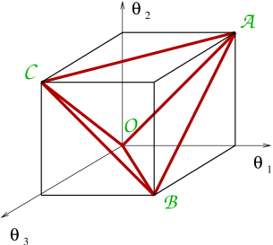
This represents supersymmetric configurations and separate an inner region, where the scalars are all massive, from an outer region, where the scalars become tachyonic. Faces, edges and vertices of the tetrahedron correspond to $\mathcal{N}=1$, $\mathcal{N}=2$ and $\mathcal{N}=4$ configurations, respectively. Notice that in our conventions, where the twists $\theta_{i}$’s are taken in the range $[0,1)$, the vertices $\mathcal{A}$, $\mathcal{B}$ and $\mathcal{C}$, and the face $(\mathcal{ABC})$ are in fact not part of the moduli space. Of course one could change conventions and choose a different parameterization without changing the physical conclusions. We will briefly return on this point in Section 5.

5 Moduli Dependence of the Kähler Metric

In this section we compute the dependence on the closed string moduli of the Kähler metric for the chiral matter in the effective action of magnetized D9-branes. Exploiting T-duality, this system can be used also for brane-worlds involving branes at angles with arbitrary open string fluxes. Our analysis generalizes previous results in the literature since we obtain an expression for the Kähler metric that is valid not only for commuting and supersymmetric fluxes on factorized torii, but also for arbitrary non-commuting and non-supersymmetric configurations on generic torii.

Let us then consider the chiral fields (4.3c) arising from $\theta$-twisted open strings connecting two (stacks of) D9-branes with generic non-commuting open string fluxes. The moduli dependence of the Kähler metric can be extracted from a 3-point function on a disk involving two open twisted matter fields $\phi^{i}$ and $\bar{\phi}^{i}$, and one closed string parameter $m$, namely

$${\cal A}_{m\bar{\phi}^{i}\phi^{i}}=\frac{1}{2\alpha^{\prime}}\,\langle V_{\bar{\phi}^{i}}\,W_{m}\,V_{\phi^{i}}\rangle~{}~{}.$$ (5.1)

The normalization in this amplitude can be obtained by using the results of Appendix A of Ref. [71], but, as we shall see, it can also be fixed independently by using the value of the tree-level mass given in (4.3c).

In order to extract the Kähler metric from ${\cal A}_{m\bar{\phi}^{i}\phi^{i}}$, a few steps must be performed. First of all, to write the results in terms of (properly normalized) field theory quantities, the open string vertices should be transformed from the canonically normalized string theory basis to the field theory basis according to

$$V_{\phi^{i}}\rightarrow\left(K_{ii}\right)^{1/2}V_{\phi^{i}}~{}~{}~{}~{},~{}~{}~{}~{}V_{\bar{\phi}^{i}}\rightarrow\left(K_{ii}\right)^{1/2}V_{\bar{\phi}^{i}}$$ (5.2)

where $K_{ii}$ is the Kähler metric for the $i$-th matter multiplet. Second, a factor of ${\rm i}$ must be introduced to transform the string scattering amplitude into the corresponding term in the effective action. The string/field theory dictionary then reads

$${\cal A}_{m\bar{\phi}^{i}\phi^{i}}={{\rm i}}\,\left(K_{ii}\right)^{-1}~{}\frac{\partial}{\partial m}~{}{\cal L}^{(2)}~{}~{},$$ (5.3)

where ${\cal L}^{(2)}$ is the quadratic part of Lagrangian of the twisted scalars with the field theory normalization. In our conventions, with a mostly plus metric, this Lagrangian reads

$${\cal L}^{(2)}=-\,K_{ii}\Big{(}\partial\bar{\phi}^{i}\cdot\partial\phi^{i}+M_{i}^{2}\,\bar{\phi}^{i}\,\phi^{i}\Big{)}~{}~{}.$$ (5.4)

Thus, from (5.3) and going to momentum space, one finds

$${\cal A}_{m\bar{\phi}^{i}\phi^{i}} ={{\rm i}}\,\left(K_{ii}\right)^{-1}\,\frac{\partial}{\partial m}\Big{[}\left(\,k_{1}\cdot k_{2}-\,M_{i}^{2}\right)K_{ii}\Big{]}\,\overline{\phi}^{i}(k_{1})\,\phi^{i}(k_{2})$$ (5.5)

$$={\rm i}\Big{[}-\frac{\partial M^{2}_{i}}{\partial m}+\big{(}k_{1}\cdot k_{2}-M^{2}_{i}\big{)}\,\frac{\partial\ln K_{ii}}{\partial m}\Big{]}\,\overline{\phi}^{i}(k_{1})\,\phi^{i}(k_{2})~{}~{},$$

where in the second line we have explicitly taken into account the dependence of the mass $M^{2}_{i}$ on the open string twists and hence on the closed string moduli.

The correlator (5.1) is a mixed open/closed string amplitude which can be computed after writing the closed string vertex operator $W_{m}$ in terms of the propagating (twisted) open string. This is done by using the boundary conditions on the disk discussed in Section 2, which imply in particular

$$V_{L}^{M}(z)=V^{M}(z)~{}~{}~{}~{},~{}~{}~{}~{}V_{R}^{M}(\bar{z})=(R_{0})^{M}_{~{}N}\,V^{N}(\bar{z})$$ (5.6)

along the compact directions, and

$$V_{L}^{\mu}(z)=V^{\mu}(z)~{}~{}~{}~{},~{}~{}~{}~{}V_{R}^{\mu}(\bar{z})=V^{\mu}(\bar{z})$$ (5.7)

along the uncompact ones. Thus, the amplitude (5.1), including the cocycle introduced in Eq. (3.8), can be written as

$${\cal A}_{m\bar{\phi}^{i}\phi^{i}}=\frac{{\rm e}^{-{\rm i}\pi\alpha^{\prime}k_{L}\cdot k_{R}}}{8\pi{\alpha^{\prime}}^{2}}\,\left[\frac{\partial}{\partial m}(G-B)\cdot R_{0}\right]_{MN}\,\langle V_{\bar{\phi}^{i}}\,V^{M}V^{N}\,V_{\phi^{i}}\rangle~{}~{}.$$ (5.8)

In the orthonormal basis (2.9), one finds

$${\cal A}_{m\bar{\phi}^{i}\phi^{i}}=\left[\frac{\partial}{\partial m}(G-B)\cdot R_{0}\right]_{MN}\,({\bf\cal E}^{-1})^{M}_{~{}a}\,({\bf\cal E}^{-1})^{N}_{~{}b}~{}{\cal A}_{(i)}^{ab}$$ (5.9)

where the indices $a,b=(i,\bar{i})=1,...6$ span the orthonormal frame, in which the monodromy matrix $R$ is diagonal and the metric $G$ is of the form (2.10), and $({\cal E}^{-1})^{M}_{~{}a}$ is the inverse of the vielbein ${\cal E}^{a}_{~{}M}$ introduced in Eq. (2.9). The matrix ${\cal A}_{(i)}$ is explicitly given by

$${\cal A}_{(i)}\equiv\left(\begin{array}[]{cc}0&A_{j(i)}\,\delta^{j{\overline{k}}}\\ {A}_{{\overline{j}}(i)}\,\delta^{{\overline{j}}k}&0\\ \end{array}\right)$$ (5.10)

where

$${A}_{j(i)}=\frac{{\rm e}^{-{\rm i}\pi\alpha^{\prime}k_{L}\cdot k_{R}}}{8\pi{\alpha^{\prime}}^{2}}\,\langle V_{\bar{\phi}^{i}}\,V^{j}V^{\overline{j}}\,V_{\phi^{i}}\rangle~{}~{},$$ (5.11)

and ${A}_{{\overline{j}}(i)}$ is given by the same expression (5.11) with $V^{j}$ and $V^{\overline{j}}$ exchanged.

The string correlator ${A}_{j(i)}$ has to be computed in the orthonormal basis, where one can use the CFT results summarized in Section 2. It is important to notice that although ${A}_{j(i)}$ depends only on the open string twists $\theta_{i}$’s, the full amplitude ${\cal A}_{m\bar{\phi}^{i}\phi^{i}}$ contains additional dependencies on the various closed string moduli through the reflection matrix $R_{0}$ and the inverse vielbein ${\cal E}^{-1}$. In summary, the computation of the string amplitude ${\cal A}_{m\bar{\phi}^{i}\phi^{i}}$ elegantly separates into two pieces: the correlator $A_{j(i)}$ and a prefactor that carries the information on the specific closed string modulus inserted and the boundary conditions. Let us start computing the first piece.

5.1 The string correlator

Here we derive the four point function ${\cal A}_{j(i)}$ defined in (5.11). For the chiral matter fields $\phi^{i}$ and $\overline{\phi}^{i}$ we take the vertex operators (4.6) and (4.9) for which the mass-shell condition is

$$\alpha^{\prime}k_{1}^{2}=\alpha^{\prime}k_{2}^{2}={\textstyle\frac{1}{2}}-{\textstyle\frac{1}{2}}\sum_{i}\left[(\theta_{j(i)}^{F})^{2}+\theta_{j}(1-\theta_{j})\right]=\frac{1}{2}\sum_{j}\epsilon^{F}_{j(i)}~{}\theta_{j}=-\alpha^{\prime}M_{i}^{2}$$ (5.12)

where

$$\epsilon_{j(i)}^{F}=\left\{\begin{array}[]{ll}~{}~{}1&i=j~{}~{},\\ -1&i\not=j~{}~{}.\end{array}\right.$$ (5.13)

For the closed string modulus, we use the vertices (3.7) with the identifications (5.6). Thus, the amplitude (5.11) can be written as

$$A_{j(i)}= -\,\frac{\overline{\phi}^{i}(k_{1})\phi^{i}(k_{2})}{4\pi{\alpha^{\prime}}}\int\frac{dx_{1}\,dx_{2}\,d^{2}z}{dV_{\rm{CKG}}}\,{\rm e}^{-{\rm i}\pi\alpha^{\prime}k_{L}\cdot k_{R}}~{}{\cal W}~{}(x_{1}-x_{2})^{-1}\,(z-\bar{z})^{-2}$$ (5.14)

$$~{}~{}\times\left[A_{\rm bos}^{j}(x_{1},z,\bar{z},x_{2}|\sigma_{\theta_{j}})-\,2\alpha^{\prime}k_{L}\cdot k_{R}\,A_{\rm ferm}^{j}(x_{1},z,\bar{z},x_{2}|{\cal S}_{\theta^{F}_{j(i)}})\right]$$

where $A_{\rm bos}^{j}$ and $A_{\rm ferm}^{j}$ are the correlators given in Eqs. (2.21) and (2.44) respectively, and ${\cal W}$ is defined by

$${\cal W} \equiv \big{\langle}{\rm e}^{{\rm i}k_{1}\cdot X(x_{1})}\,{\rm e}^{{\rm i}k_{L}\cdot X(z)}\,{\rm e}^{{\rm i}k_{R}\cdot X(\bar{z})}\,{\rm e}^{{\rm i}k_{2}\cdot X(x_{2})}\big{\rangle}\,\prod_{j=1}^{3}\big{[}\langle\sigma_{-\theta_{j}}(x_{1})\sigma_{\theta_{j}}(x_{2})\rangle\,\langle{\cal S}_{-\theta^{F}_{j(i)}}(x_{1}){\cal S}_{\theta^{F}_{j(i)}}(x_{2})\rangle\big{]}$$ (5.15)

$$= (x_{1}-x_{2})^{-1}\,\omega^{\alpha^{\prime}(t+M_{i}^{2})}\,(1-\omega)^{\alpha^{\prime}s}$$

in terms of the anharmonic ratio

$$\omega=\frac{(x_{1}-z)(\bar{z}-x_{2})}{(x_{1}-\bar{z})(z-x_{2})}~{}~{}~{}~{}~{}(~{}|\omega|=1~{})~{}~{},$$ (5.16)

and the Mandelstam variables

$$s =(k_{1}+k_{2})^{2}=(k_{L}+k_{R})^{2}~{}~{},$$ (5.17)

$$u =(k_{1}+k_{L})^{2}=(k_{2}+k_{R})^{2}~{}~{},$$

$$t =(k_{1}+k_{R})^{2}=(k_{2}+k_{L})^{2}~{}~{},$$

with

$$k_{L}^{2}=k_{R}^{2}=0~{}~{},~{}~{}k_{1}^{2}=k_{2}^{2}=-M_{i}^{2}~{}~{},~{}~{}s+t+u=-2M_{i}^{2}~{}~{}.$$ (5.18)

In the following we keep the open strings on-shell, but we take the closed string off-shell. If also the closed string were on-shell, we would have $u=t$ and $s=0$. In our off-shell extension, instead, we retain the relation $u=t$ but keep $s$ non-vanishing, i.e. we take $s=-2(t+M_{i}^{2})$.

Finally, in (5.14) the open string punctures $x_{1}$ and $x_{2}$ are integrated on the real axis, while the closed string variable $z$ is integrated on the upper-half complex plane, modulo the $\mathrm{Sl}(2,\mathbb{R})$ projective invariance which is fixed by the Conformal Killing Group volume $dV_{\rm{CKG}}$. Using this fact, one can show that

$$\frac{dx_{1}\,dx_{2}\,d^{2}z}{dV_{{\rm CKG}}}\,(x_{1}-x_{2})^{-2}\,(z-\overline{z})^{-2}=(1-\omega)^{-2}d\omega$$ (5.19)

and thus the amplitude $A_{j(i)}$ in (5.14) becomes

$$A_{j(i)}=-\frac{\overline{\phi}^{i}(k_{1})\phi^{i}(k_{2})}{4\pi\alpha^{\prime}}\,{\rm e}^{-{\rm i}\,\pi\alpha^{\prime}s/2}\!\int_{\mathcal{C}}d\omega~{}\omega^{-\theta_{j}-\alpha^{\prime}s/2}(1-\omega)^{\alpha^{\prime}s-2}\Big{[}1-\theta_{j}(1-\omega)-\alpha^{\prime}s\,\omega^{\theta_{j}-\theta^{F}_{j(i)}}\Big{]}~{}~{}.$$ (5.20)

Notice that the original integral over $z$ takes into account all possible orderings of the closed string insertion along the open string boundary. In the $\omega$-variable this translates into a closed integral $\mathcal{C}$ along the unit circle $|\omega|=1$ clockwise oriented. The integrand in (5.20) has a branch cut along the positive real axis and thus the contour $\mathcal{C}$ must be deformed in order to circumvent the cut singularity. So we have to perform the integration just below the cut for $\omega\in[0,1]$ and then subtract the contribution from above the cut for $\omega\in{\rm e}^{-2\pi{\rm i}}[0,1]$. Using the definition of the Euler $B$-function, the amplitude (5.20) takes the form

$$A_{j(i)} =\,-\,\frac{{\rm i}\,\overline{\phi}^{i}(k_{1})\phi^{i}(k_{2})}{2\pi\alpha^{\prime}}\,{\rm e}^{{\rm i}\pi\theta_{j}}\,\sin\Big{[}\pi\big{(}\theta_{j}+{\alpha^{\prime}s}/{2}\big{)}\Big{]}\,\Bigg{\{}B(1-\theta_{j}-\alpha^{\prime}s/2,\alpha^{\prime}s-1)$$ (5.21)

$$~{}~{}~{}~{}~{}~{}-\theta_{j}\,B(1-\theta_{j}-\alpha^{\prime}s/2,\alpha^{\prime}s)-\alpha^{\prime}s\,B(1-\theta^{F}_{j(i)}-\alpha^{\prime}s/2,\alpha^{\prime}s-1)\Bigg{\}}$$

$$=\,-\frac{{\rm i}\,\overline{\phi}^{i}(k_{1})\phi^{i}(k_{2})}{4\pi\alpha^{\prime}}\,\epsilon_{j(i)}^{F}\,{\rm e}^{{\rm i}\pi\theta_{j}}\,\sin\Big{[}\pi\big{(}\theta_{j}+{\alpha^{\prime}s}/{2}\big{)}\Big{]}\,\,\frac{\Gamma(\alpha^{\prime}s+1)\Gamma(1-\theta_{j}-\alpha^{\prime}{s}/{2})}{\Gamma(1-\theta_{j}+\alpha^{\prime}{s}/{2})}$$

where $\epsilon_{j(i)}^{F}$ are the signs introduced in (5.13).

In order to extract information about the low energy effective action, a few further steps must be performed. First we have to expand our result (5.21) in powers of $\alpha^{\prime}s$, then take the limit $\alpha^{\prime}\rightarrow 0$ keeping the mass $M_{i}$ fixed: in this way the first two terms in such expansion yield the mass and the kinetic terms for the scalar fields, if we use the relation $s=2k_{1}\cdot k_{2}-2M_{i}^{2}$. Then, we get

$$A_{j(i)}=-\frac{{\rm i}\,\overline{\phi}^{i}(k_{1})\phi^{i}(k_{2})}{4\pi\alpha^{\prime}}\,\epsilon^{F}_{j(i)}\,{\rm e}^{{\rm i}\pi\theta_{j}}\sin(\pi\theta_{j})(1-\frac{1}{2}\,\alpha^{\prime}s\,\rho_{j})+\,{\cal O}\left(\alpha^{\prime}s^{2}\right)$$ (5.22)

with

$$\rho_{j}=\psi(1-\theta_{j})+\psi(\theta_{j})+2\gamma_{E}~{}~{}.$$ (5.23)

Here $\gamma_{E}$ is the Euler-Mascheroni constant and $\psi(x)=d\,{\rm ln}\Gamma(x)/dx$. In writing $\rho_{j}$ as in (5.23), we have used the identity $\psi(1-\theta_{j})=\psi(\theta_{j})+\pi\cos(\pi\theta_{j})/\sin(\pi\theta_{j})$. Notice that the result (5.22) holds independently from supersymmetry, i.e. it is valid both for $M_{i}=0$ and $M_{i}\not=0$, and is exact in $\alpha^{\prime}$.

Proceeding as above, one can show that the amplitude ${A}_{{\overline{j}}(i)}$ is given by the same expression (5.22) with ${\rm e}^{{\rm i}\pi\theta_{j}}$ replaced by ${\rm e}^{-{\rm i}\pi\theta_{j}}$.

5.2 Identifying the Kähler metric

In this section we finally extract the Kähler metric $K_{ii}$ from the string amplitude ${\cal A}_{m\bar{\phi}^{i}\phi^{i}}$. In order to achieve this goal, we show that the string amplitude can be written in the form (5.5) from which the expression of the Kähler metric can be read off. Let us define for convenience

$$h_{j(i)}=\frac{\overline{\phi}^{i}(k_{1})\phi^{i}(k_{2})}{4\pi\alpha^{\prime}}\,\epsilon^{F}_{j(i)}\,\big{(}1-\frac{1}{2}\alpha^{\prime}\,s\,\rho_{j}\big{)}$$ (5.24)

and introduce the matrix

$${\cal H}_{(i)}=\left(\begin{array}[]{cc}h_{j(i)}\,\delta^{j}_{~{}k}&0\\ 0&-h_{\bar{j}(i)}\,\delta^{\bar{j}}_{~{}\bar{k}}\\ \end{array}\right)~{}~{}~{}~{}{\rm with}~{}~{}~{}~{}h_{\bar{j}(i)}={\overline{h}}_{j(i)}~{}~{}.$$ (5.25)

Then, after simple manipulations one sees that Eq. (5.10) can be rewritten as

$${\cal A}_{(i)}=\frac{1}{2}\,{\cal G}^{-1}\,({\cal R}^{-1}-1)\,{\cal H}_{(i)}~{}~{}.$$ (5.26)

Plugging this back into Eq. (5.9), one finally finds

$${\cal A}_{m\bar{\phi}^{i}\phi^{i}} ={\rm tr}\left[{}^{t}{\cal E}^{-1}\,\frac{\partial}{\partial m}(G-B)~{}R_{0}~{}{\cal E}^{-1}~{}{}^{t}{\cal A}_{(i)}\right]$$ (5.27)

$$=\frac{1}{2}\,{\rm tr}\left[{}^{t}{\cal E}^{-1}\,\frac{\partial}{\partial m}(G-B)~{}(R_{\pi}-R_{0})~{}{\cal E}^{-1}{\cal H}_{(i)}~{}{\cal G}^{-1}~{}\right]$$

$$=\frac{1}{2}\sum_{j=1}^{3}\Bigg{[}\left(\mathcal{E}\,G^{-1}\,\frac{\partial(G-B)}{\partial m}\,\left(R_{\pi}-R_{0}\right)\,\mathcal{E}^{-1}\right)_{jj}-{\rm h.c.}\Bigg{]}\,h_{j(i)}~{}~{}.$$

At this point the crucial observation is that the term multiplying $h_{j(i)}$ in the above expression can be written as a total derivative with respect to $m$. This fact follows from the non-trivial identity (3.12), whose proof is presented in Appendix A. Using this identity in (5.27), we find

$${\cal A}_{m\bar{\phi}^{i}\phi^{i}}=2\pi{{\rm i}}\,\sum_{j=1}^{3}h_{j(i)}\,\frac{\partial\theta_{j}}{\partial m}~{}~{}.$$ (5.28)

Then, inserting the relation $s=2k_{1}\cdot k_{2}-2M_{i}^{2}$ in the explicit expression of $h_{j(i)}$ given in (5.24), we get

$$2\pi h_{j(i)} =\epsilon^{F}_{j(i)}\,\left[\frac{1}{2\alpha^{\prime}}-\frac{1}{2}\,\big{(}k_{1}\cdot k_{2}-M_{i}^{2}\big{)}\,\rho_{j}\right]\,\overline{\phi}^{i}(k_{1})\phi^{i}(k_{2})$$ (5.29)

$$=\Bigg{[}\frac{\epsilon^{F}_{j(i)}}{2\alpha^{\prime}}+(k_{1}k_{2}-M_{i}^{2})\frac{d}{d\theta_{j}}\ln\Big{(}{\rm e}^{-2\gamma_{E}\theta_{j}}\,\frac{\Gamma(1-\theta_{j})}{\Gamma(\theta_{j})}\Big{)}^{\epsilon^{F}_{j(i)}/2}\Bigg{]}\,\overline{\phi}^{i}(k_{1})\phi^{i}(k_{2})$$

where in the last step we have used the definition (5.23) for $\rho_{j}$. From the analysis of the spectrum we know the value of the tree-level mass $M_{i}^{2}=-\frac{1}{2\,\alpha^{\prime}}\,\sum_{j}\epsilon^{F}_{j(i)}\,\theta_{j}$, which allows to interpret the first term in the equation above as $-\partial M_{i}^{2}/\partial\theta_{j}$. Notice that this is a way to fix unambiguously the overall normalization of the string amplitude and thus also the power of the Kähler metric below. At this point we can use Eq. (5.28) to write the amplitude ${\cal A}_{m\bar{\phi}^{i}\phi^{i}}$ in the form of Eq. (5.5) and read the explicit form of $K$

$$K_{ii}(\theta)={\rm e}^{2\gamma_{E}\,\alpha^{\prime}M_{i}^{2}}\,\prod_{j=1}^{3}\left(\frac{\Gamma(1-\theta_{j})}{\Gamma(\theta_{j})}\right)^{\epsilon^{F}_{j(i)}/2}~{}~{}.$$ (5.30)

Formula (5.30) is the main result of this paper and, as we discuss below, it generalizes previous results in the literature. It displays the full moduli dependence of the Kähler metric of the chiral matter coming from the $\theta$-twisted open strings and holds for an arbitrary brane setup in presence of generic non-commuting fluxes. Notice that the result (5.30) holds independently on whether supersymmetry is preserved or broken, i.e. it is valid even when $M_{i}\neq 0$. Remarkably, the Kähler metric is always determined by a simple function of the twists $\theta_{i}$. It is worth stressing that in this derivation it is useful to keep $M_{i}\neq 0$ in order to fix the overall normalization of the string amplitude, including the sign, and hence to determine in the end the exact power in (5.30).

Notice that Eq. (5.30) is exact in $\alpha^{\prime}$. The field-theory result is obtained by taking the limit $\alpha^{\prime}\rightarrow 0$ with $M_{i}^{2}$ fixed. In this limit the exponential vanishes and the Kähler metric entering the field-theory Lagrangian finally reads

$$K^{(0)}_{ii}=\lim_{\alpha^{\prime}\to 0}K_{ii}(\theta)=\sqrt{\frac{\Gamma(1-\theta^{(0)}_{i})}{\Gamma(\theta^{(0)}_{i})}}\,\prod_{j\not=i}\sqrt{\frac{\Gamma(\theta^{(0)}_{j})}{\Gamma(1-\theta^{(0)}_{j})}}$$ (5.31)

where $\theta^{(0)}_{j}=\lim_{\alpha^{\prime}\to 0}\theta_{j}$ as in (4.4), and the signs $\epsilon^{F}_{j(i)}$ for the scalar $\phi^{i}$ have been made explicit.

Some comments are in order at this point. First we notice that if we start from a non-supersymmetric set of $\theta_{i}$’s, the only way to decouple one of the twisted scalars from the string scale is to suppose that the $\theta_{i}^{(0)}$’s satisfy a supersymmetric constraint, as is clear from the mass formula (4.5). This means that one is considering a particular point in Fig. 1 which is at a “stringy” distance from a given supersymmetric configuration, in such a way that one scalar can survive in the field theory limit $\alpha^{\prime}\to 0$ with a finite mass. As we will discuss in the next section this breaking can be interpreted at the field theory level as coming from a non-vanishing v.e.v. of a Fayet-Iliopoulos term.

Notice that in our derivation we have chosen a set of conventions for which the ${\cal N}=4$ supersymmetric point included in our $\theta$-space is the vertex ${\cal O}$ of the tetrahedron in Fig. 1. However, our results hold for any other choice. For instance, we could repeat the above analysis with different conventions and consider a field theory where the starting point is another ${\cal N}=4$ vertex of the tetrahedron in Fig. 1. In this case, the scalar becoming massless on the outer wall $({\cal ABC})$ would now enter the low energy effective spectrum and its Kähler metric would be

$$K^{(0)}=\prod_{j=1}^{3}\left(\frac{\Gamma(1-\theta^{(0)}_{j})}{\Gamma(\theta^{(0)}_{j})}\right)^{1/2}~{}~{}.$$ (5.32)

This is the scalar that is usually considered in the literature. However, we point out that the exponent in Eq. (5.32) has a different sign as compared to previous findings, but it agrees with the result of Ref. [54]. In the Heterotic computations [49] the Kähler metric for the scalar fields is derived from a four point amplitude on the sphere. One may wonder why in models with open strings it is possible to derive this result from a three point function and, conversely, what rôle a four point function would have in this context. However, at the CFT level, the insertion of a closed string on a disk is equivalent to the insertion of two open vertices. Thus the Koba-Nielsen integrals are those also considered in Ref. [49]. Of course, the space-time interpretation and kinematics are those of a three point function. Thus, to get a meaningful result, it is important to give a prescription to continue the string amplitude off-shell, as we do, at least in the field theory limit. It would be very interesting to check this off-shell prescription by computing disk diagrams with the insertion of two moduli vertices and see whether the results are consistent with Eq. (5.30). This is a challenging computation and some preliminary results were presented in [21] for the factorized and commuting case. The authors of [21] suggested that the differential equations derived from the three point function should actually be modified to agree with the results coming from higher point amplitudes. Here we seem to have no room for modifications of this type. We present a check of this in Appendix B; there we focus on the untwisted scalars where it is possible to compare the result with the Born-Infeld action and we find complete agreement. So we believe that our off-shell prescription is able to capture the full NS-NS moduli dependence of the metric for all scalar fields.

5.3 Commuting cases

To make contact with previous results in the literature, here we illustrate our results in the simplest situation where the flux and the reflection matrices $R_{\sigma}$ commute. Representatives of this commuting case are the branes with “diagonal fluxes ” discussed in Section 3.1. Using the results derived there (but dropping for simplicity the index $i$ labeling the three torii $\mathcal{T}^{2}_{i}$), one can explicitly verify that derivatives of the twist parameter satisfy Eq. (3.12). Indeed, from (3.17) it follows that

$$2\pi{\rm i}\,\frac{\partial\theta}{\partial T}=\frac{f_{\pi}-f_{0}}{(T-f_{\pi})(T-f_{0})}~{}~{}.$$ (5.33)

Using Eqs. (3.13) – (3.15) it is not difficult to check that the general relation (3.12) correctly reproduces Eq. (5.33) (see Appendix A.1 for further details).

As is well-known, a T-duality along the $y$ direction of the torus $\mathcal{T}^{2}$ corresponds to the exchange $T\leftrightarrow-1/U$, and the magnetized branes of the type IIB theory become branes of type IIA intersecting at angles. A careful analysis of the boundary conditions (2.5) reveals that under this T-duality the reflection matrices (3.16) transform into

$$\mathcal{R}^{\prime}_{\sigma}=\begin{pmatrix}0&-\frac{1+\overline{U}\,f_{\sigma}}{1+U\,f_{\sigma}}\\ -\frac{1+U\,f_{\sigma}}{1+\overline{U}\,f_{\sigma}}&0\end{pmatrix}~{}~{}.$$ (5.34)

Clearly $\mathcal{R}^{\prime}_{0}$ and $\mathcal{R}^{\prime}_{\pi}$ commute with each other. These T-dual reflection matrices depend on the complex structure $U$ and the quantized magnetic fluxes $f_{\sigma}$, but are independent of the Kähler modulus $T$, in contrast to the original matrices $\mathcal{R}_{\sigma}$ of Eq. (3.16). The monodromy matrix $\mathcal{R}^{\prime}=\big{(}{\mathcal{R}^{\prime}}_{\pi}\big{)}^{-1}\mathcal{R}^{\prime}_{0}$ of the T-dual theory is of the form $\mathcal{R}^{\prime}=\mathrm{diag}\,\left({\rm e}^{2\pi{\rm i}\theta^{\prime}},{\rm e}^{-2\pi{\rm i}\theta^{\prime}}\right)$ with

$${\rm e}^{2\pi{\rm i}\theta^{\prime}}=\frac{1+U\,f_{\pi}}{1+\overline{U}\,f_{\pi}}\,\frac{1+\overline{U}\,f_{0}}{1+U\,f_{0}}~{}~{},$$ (5.35)

which is the direct T-dual transform of Eq. (3.17). In this case the twist $\theta^{\prime}$ represents the intersecting angle between the two D-branes to which the open string is attached. If we take one of the branes to lie on the $x$ axis, i.e. if we set $f_{0}=0$, then Eq. (5.35) can be simply rewritten as

$$\tan(\pi\theta^{\prime})=\frac{U_{2}\,p}{q+U_{1}p}$$ (5.36)

where the quantization condition $f_{\pi}=p/q$ has been used. This is the usual relation of the angle between two D-branes with the complex structure moduli of the two-dimensional torus $\mathcal{T}_{2}$ in which they intersect, a relation that can be easily understood and derived also in geometrical terms. From Eq. (5.36) it follows that

$$2\pi{\rm i}\,\frac{\partial\theta^{\prime}}{\partial U}=\frac{2p}{(q+U\,p)}~{}~{},$$ (5.37)

which again agrees with the general result (3.12). Notice that indeed Eqs. (5.33) and (5.37) are related by the T-duality map $T\Leftrightarrow-\frac{1}{U}$. More generally, under a T-duality transformation $\bar{X}^{M}=T^{M}{}_{N}\bar{X}^{N}$, it can be shown that the flux matrices transform as [72]

$$\left[R_{\sigma}^{\prime}(m^{\prime})\right]^{M}{}_{N}=\left[R_{\sigma}(m(m^{\prime}))\right]^{M}{}_{P}\,T^{P}{}_{N}$$ (5.38)

where $m$ and $m^{\prime}$ the T-dual moduli and the $d\times d$ matrix $T^{M}{}_{N}$ satisfies $T_{MN}=T_{NM}$ and $T^{2}=1$. The dependence on this matrix $T$ cancels out in the monodromy matrix $R$ and therefore open string twists in T-dual theories are simply related by replacing $m\Leftrightarrow m^{\prime}$. The case of the T-duality in the $y$ direction of the two torus $\mathcal{T}^{2}$ discussed above is just an explicit example of this more general statement.

5.4 Supersymmetry breaking by $D$- and $F$-terms

In presence of generic fluxes (or angles) supersymmetry may be broken by $D$- and $F$-terms. Here we would like to analyze explicitly from a string theory point of view these mechanisms starting from the one produced by $D$-terms.

Let us then compute the v.e.v. of the auxiliary fields $D$ of the gauge vector multiplet for our system of magnetized branes with generic fluxes. Since the chiral matter arises from open strings stretched between two (stacks of) D9-branes, we should consider both the $D$ field of the gauge multiplet for the branes at $\sigma=0$ and the $D$ field on the branes at $\sigma=\pi$, and then focus on their respective $\mathrm{U}(1)$ parts which are the only ones that can get a v.e.v. In particular we should compute from string diagrams the difference

$$\langle D\rangle_{\pi}-\langle D\rangle_{0}$$ (5.39)

and show that, as expected, it corresponds to a mass for the twisted chiral matter. Just like we did for the Kähler metric, we will actually compute the derivative of the above quantity with respect to a closed string modulus $m$, rather than the v.e.v.’s themselves. More precisely we consider a disk amplitude between a vertex operator $V_{D}$ for the auxiliary field $D$ and a closed string vertex operator $W_{m}$ for the modulus $m$, and read from it the v.e.v. of the $D$ fields according to

$$\mathcal{A}_{mD}\equiv\langle W_{m}\,V_{D}\rangle_{\pi}-\langle W_{m}\,V_{D}\rangle_{0}={\rm i}\,\frac{\partial}{\partial m}\Big{(}\langle D\rangle_{\pi}-\langle D\rangle_{0}\Big{)}$$ (5.40)

where the subscripts $0$ and $\pi$ on the string correlators indicate that the appropriate boundary conditions for the branes at $\sigma=0$ and $\sigma=\pi$ should be enforced. Auxiliary fields are realized in string theory in terms of non-BRST invariant operators in the 0-superghost picture (see, for example, Ref. [73] for details and Ref. [74] for some recent applications in mixed open/closed string amplitudes) given by

$$V_{D}(z)=\frac{1}{2}\,\xi_{(i)MN}\,:\Psi^{M}(z)\Psi^{N}(z):$$ (5.41)

where $\xi_{(i)}$ is the imaginary part of the Kähler form of the internal torus. The label $(i)$ specifies along which ${\cal N}=1$ supersymmetry, out of the starting ${\cal N}=4$, the auxiliary field under consideration is aligned. In the complex basis (2.9) we have

$${}^{t}{\cal E}^{-1}\,\xi_{(i)}\,{\cal E}^{-1}=\left(\begin{array}[]{cc}0&{\epsilon}_{j(i)}^{F}\,\delta_{j\bar{k}}\\ -{\epsilon}_{j(i)}^{F}\,\delta_{\bar{j}k}&0\\ \end{array}\right)$$ (5.42)

where are the signs introduced in Eq. (5.13). In writing $\xi_{(i)}$ in this form we use the fact that in the orthonormal basis the metric of the torus is of the form (2.10) and rearrange rows and columns in order to ensure that the twists $\theta_{i}$’s are all positive.

Since the vertex $V_{D}$ is in the 0-superghost picture, we need to take the closed string vertex $W_{m}$ in the ($-1,-1$) picture, where it is given by Eq. (3.9) with

$$V_{L}^{M}(z)=\frac{1}{\sqrt{2}}\,{\rm e}^{-\varphi_{L}(z)}\,\Psi_{L}^{M}(z)~{}~{}~{}~{}{\rm and}~{}~{}~{}~{}V_{R}^{M}(\overline{z})=\frac{1}{\sqrt{2}}\,{\rm e}^{-\varphi_{R}(\overline{z})}\,\Psi_{R}^{M}(\overline{z})~{}~{}.$$ (5.43)

As already mentioned, the amplitude $\mathcal{A}_{mD}$ receives contributions from insertions in the disks at $\sigma=0$ and $\sigma=\pi$ with boundary conditions parameterized by the reflection matrix $R_{\sigma}$, so that the identifications of the left and right moving parts of the closed string with the propagating (untwisted) open string are

$$V_{L}^{M}(z)=V^{M}(z)~{}~{}~{}~{}{\rm and}~{}~{}~{}~{}V_{R}^{M}(\overline{z})=(R_{\sigma})^{M}_{~{}N}V^{N}(\overline{z})~{}~{}.$$ (5.44)

Collecting all pieces one finds

$${\cal A}_{mD} =\frac{1}{16\pi\alpha^{\prime}}\,\xi_{(i)PQ}\left[\frac{\partial}{\partial m}(G-B)\,(R_{\pi}-R_{0})\right]_{MN}$$ (5.45)

$$~{}~{}~{}~{}\times\int\frac{dx\,d^{2}z}{dV_{\rm{CKG}}}~{}\Big{\langle}{\rm e}^{-\varphi(z)}\,\Psi^{M}(z)~{}{\rm e}^{-\varphi(\overline{z})}\,\Psi^{N}(\overline{z})~{}:\Psi^{P}\Psi^{Q}:(x)\Big{\rangle}$$

$$=\frac{1}{8\pi\alpha^{\prime}}\,{\rm tr}\,\left[G^{-1}\,\xi_{(i)}\,G^{-1}\frac{\partial}{\partial m}(G-B)\,(R_{\pi}-R_{0})\right]~{}~{}.$$

Notice that the full dependence on world-sheet positions cancels in the integrand in agreement with the $\mathrm{Sl}(2,\mathbb{\mathbb{R}})$ invariance. That only the $U(1)$ part of $V_{D}$ contributes to ${\cal A}_{mD}$ is clear since this amplitude is proportional to the trace of the Chan-Paton factor carried by the $D$-vertex. Finally, using (5.42) to rewrite the polarization $\xi_{(i)}$ in the orthonormal basis and exploiting the non-trivial identity (3.12), one finds

$${\cal A}_{mD} =-\frac{1}{8\pi\alpha^{\prime}}\,\sum_{j=1}^{3}\Bigg{[}\left(\mathcal{E}\,G^{-1}\,\frac{\partial(G-B)}{\partial m}\,\left(R_{\pi}-R_{0}\right)\,\mathcal{E}^{-1}\right)_{jj}-{\rm h.c.}\Bigg{]}\,{\epsilon}_{j(i)}^{F}$$ (5.46)

$$=-\,\frac{{\rm i}}{2\alpha^{\prime}}\,\sum_{j=1}^{3}{\epsilon}_{j(i)}^{F}\,\frac{\partial\theta_{j}}{\partial m}\,=\,{\rm i}\,\frac{\partial M_{i}^{2}}{\partial m}~{}~{}.$$

Comparing with Eq. (5.40), we see that indeed $M_{i}^{2}=\langle D\rangle_{\pi}-\langle D\rangle_{0}$, thus proving that the twisted scalars $\phi^{i}$ become massive when the $D$ fields acquire a v.e.v. This calculation shows also in a very explicit way that the subleading terms $\epsilon_{i}$ in the open string twists, defined in (4.4), which responsible for the scalar mass, have the interpretation of Fayet-Iliopoulos parameters in the effective low-energy theory.

In a similar way one can compute also the $F$-terms, i.e. the v.e.v. of the auxiliary fields $F^{i}$ and $F^{\bar{i}}$ of the adjoint chiral multiplets of the untwisted sector. Their corresponding vertex operators are of the form

$$V_{F^{i}}(z)=\frac{1}{2}\,\zeta^{i}_{MN}\,:\Psi^{M}(z)\Psi^{N}(z):~{}~{}~{}~{}{\rm and}~{}~{}~{}~{}V_{F^{\bar{i}}}(z)=\frac{1}{2}\,\zeta^{\bar{i}}_{MN}\,:\Psi^{M}(z)\Psi^{N}(z):$$ (5.47)

where the polarizations $\zeta^{i}$ and $\zeta^{\bar{i}}$, in the complex orthonormal basis, are

$${}^{t}{\cal E}^{-1}\,\zeta^{i}\,{\cal E}^{-1}\sim\left(\begin{array}[]{cc}0&0\\ 0&\delta^{i\bar{j}}\,\epsilon_{\bar{j}\bar{k}\bar{\ell}}\\ \end{array}\right)~{}~{}~{}~{}{\rm and}~{}~{}~{}~{}{}^{t}{\cal E}^{-1}\,\zeta^{\bar{i}}\,{\cal E}^{-1}\sim\left(\begin{array}[]{cc}\delta^{\bar{i}j}\,\epsilon_{jk\ell}&0\\ 0&0\\ \end{array}\right)~{}~{}.$$ (5.48)

Notice that unlike the polarization (5.42) of the $D$ vertex operator, these polarizations have non vanishing entries in the diagonal blocks when they are expressed in the orthonormal frame.

The v.e.v. of $F^{i}$ and $F^{\bar{i}}$ can be obtained from the string amplitudes $\mathcal{A}_{mF^{i}}$ and $\mathcal{A}_{mF^{\bar{i}}}$, which have the same form as (5.45) but with $\xi_{(i)}$ replaced by $\zeta^{i}$ and $\zeta^{\bar{i}}$. Due to the structure of these polarizations, we immediately see that in the interesting case where fluxes are of type $(1,1)$ and $\partial_{m}(G-B)$ is block off-diagonal, there is no F-term since the trace in (5.45) vanishes. In this way we see that fluxes of type (1,1) do not give rise to any $F$-term and hence do not break supersymmetry. On the contrary, fluxes of the type (2,0), which correspond to a $\partial_{m}(G-B)$ with non-vanishing entries also in the diagonal blocks, do produce an non-vanishing $F$-term amplitude and hence induce a non-vanishing v.e.v. for these auxiliary fields. From the structure of the vertex operators (5.47) it is easy to realize that in the field theory limit $F^{i}$ and $F^{\bar{i}}$ do not couple to the chiral fields of the twisted sector, and thus the presence of a non-vanishing $F$-term does not break supersymmetry there. However, supersymmetry will be broken by these $F$-terms in other sectors, for example in the bulk.

6 Relation with the Yukawa Couplings

The Yukawa couplings among the fields arising from intersecting or magnetized brane worlds admit a nice stringy description [18], which represents actually one of the strong points of such constructions. We focus on the couplings between chiral fermions and scalars all arising from twisted strings. In this stringy description, the couplings appearing in the Yukawa terms of the effective action have the form

$$Y_{IJK}=\mathcal{A}_{IJK}\,\mathcal{W}_{IJK}~{}~{},$$ (6.1)

where $I,J,K$ are generic indices denoting the various scalars and fermions, which we will specify better in the cases we are actually concerned with. Here $\mathcal{W}_{IJK}$ we denote classical contributions, which in the case of intersecting branes [18, 19, 20, 21] are given by world-sheet instantons bordered by the intersecting branes. In this context, since the replica families of fields arise from multiple intersections of the branes, the different areas of the minimal world-sheet connecting different intersections provide naturally an exponential hierarchy of couplings, see Fig. 2a).

Figure 2: a) Classical contributions $\mathcal{W}_{IJK}$ to the Yukawa couplings in intersecting D-brane models. b) Quantum contributions $\mathcal{A}_{IJK}$ are given by string correlators

The (string) quantum contributions $\mathcal{A}_{IJK}$ to the couplings are instead provided by the correlator of the twisted emission vertices of a scalar $V_{\phi^{I}}$ (from the NS sector of a twisted string) and of two fermions $V_{\lambda^{J}}$ and $V_{\lambda^{K}}$, from the R sector of two other twisted strings, see Fig. 2b)

$$\mathcal{A}_{IJK}=\langle V_{\phi^{I}}V_{\lambda^{J}}V_{\lambda^{K}}\rangle\propto\int\frac{dx_{1}dx_{2}dx_{3}}{dV_{\mathrm{CKG}}}\langle V_{\phi^{I}}(x_{1})V_{\lambda^{J}}(x_{2})V_{\lambda^{K}}(x_{3})\rangle~{}~{}.$$ (6.2)

A three-point CFT correlator is determined from conformal invariance up to a constant; since the vertices have conformal dimension 1, this structure constant coincides directly with the string amplitude

$$\langle V_{\phi^{I}}(x_{1})V_{\lambda^{J}}(x_{2})V_{\lambda^{K}}(x_{3})\rangle=\frac{\mathcal{A}_{IJK}}{\prod_{a,b=1}^{3}(x_{a}-x_{b})}~{}~{}.$$ (6.3)

The world-sheet dependence from the $x_{a}$, indeed, just cancels in the amplitude Eq. (6.2) against the Jacobian to gauge-fix $\mathrm{SL}(2,\mathbb{R})$ invariance.

We consider $\mathcal{N}=1$ configurations, in which supersymmetry may be broken, as we have just seen, by the presence of D-terms. In $\mathcal{N}=1$ theories, the Yukawa couplings are encoded in the superpotential. In truth, our effective action is an $\mathcal{N}=1$ supergravity, and beside the twisted matter multiplets $\Phi^{I}$ we have matter multiplets originating from the closed string sector, including the moduli scalars $m$. As we did for the Kähler potential, though, we presently consider the moduli $m$ as fixed and expand the superpotential in the open string multiplets $\Phi^{I}$. The cubic level of this expansion

$$W=W_{IJK}(m)\,\Phi^{I}\Phi^{j}\Phi^{K}~{}~{},$$ (6.4)

displays the holomorphic couplings $W_{IJK}$ when the moduli are written in the appropriate complex basis. These couplings govern the Yukawa terms involving one scalar and two fermions from these multiplets. They, however, do not directly represent the physical Yukawa couplings $Y_{IJK}$ because in the $\mathcal{N}=1$ Lagrangian the chiral multiplet fields have non-canonical kinetic terms involving the Kähler metric $K_{IJ}(m)$. To read off the physical couplings we have to rescale the fields: $\Phi^{I}\to(K_{II})^{-1/2}\,\Phi^{I}$, see the discussion before (5.2), getting

$$Y_{IJK}=\Big{[}K_{II}K_{JJ}K_{KK}\Big{]}^{-1/2}\,W_{IJK}~{}~{}.$$ (6.5)

For $\mathcal{N}=1$ effective theories realized in Heterotic string compactifications, a powerful non-renormalization theorem [56] asserts that the superpotential $W$ gets no perturbative $\alpha^{\prime}$ corrections. It is likely that the same non-renormalization property holds also in the brane-world context. If this is the case, we should identify the holomorphic couplings $W_{IJK}$ with the classical world-sheet instanton contributions

$$W_{IJK}=\mathcal{W}_{IJK}~{}~{},$$ (6.6)

since these contributions depend non-perturbatively on $\alpha^{\prime}$: $\mathcal{W}_{IJK}\sim{\rm e}^{S/\alpha^{\prime}}$. On the other hand, the string amplitude $\mathcal{A}_{IJK}$ with three twisted vertices can be certainly expanded perturbatively in $\alpha^{\prime}$ and so can not contribute to the form of the superpotential. It then follows from Eqs. (6.1) and (6.5) that $\mathcal{A}_{IJK}$ should factorize in term of the Kähler metrics for the involved fields, namely

$$\mathcal{A}_{IJK}=\Big{[}K_{II}K_{JJ}K_{KK}\Big{]}^{-1/2}~{}~{}.$$ (6.7)

This remarkable statement should be checked against the direct computation of the string correlator $\mathcal{A}_{IJK}$. Let us analyze this problem and, to begin with, let us recall which chiral multiplets we consider and set up a convenient notation.

As we discussed in Section 4, an open string stretching between two different D-branes is characterized by the eigenvalues $\theta_{i}$ ($i=1,2,3$) of its monodromy $R(\theta)$. It contains in its NS spectrum three different scalars $\phi^{i}$ which can be retained in the effective theory also for non-trivial values of the twists. These are the states of Eq. (4.3c); their mass is given in Eqs. (4.3c-4.5), and the corresponding emission vertices in Eq. (4.6). For $\sum_{j\not=i}\theta_{j}-\theta_{i}=0$, the scalar $\phi^{i}$ is massless and sits in a chiral $\mathcal{N}=1$ multiplet with the massless chiral fermion $\lambda$ from the R sector. The latter is present for any value of the $\theta$’s, and its emission vertex was written in Eq. (4.11).

In a given model of magnetized or intersecting D-branes, there are various types of branes, and many open strings sectors associated to various pairs of different D-branes. These sectors are distinguished by the corresponding monodromy $R(\theta)$ and its eigenvalues, the twists $\theta_{j}$. We can thus label the chiral multiplets as $\Phi^{i}_{\theta}$. The corresponding Kähler metric is evidently diagonal in the space of different open string sectors, and also with respect to the type $i$ of scalars under consideration. We choose for it the notation $K_{ii}(\theta)$. The string amplitude computing the quantum part of the Yukawa couplings among three such chiral multiplets $\Phi^{i}_{\theta}$, $\Phi^{j}_{\nu}$ and $\Phi^{k}_{\omega}$ is

$$\mathcal{A}_{ijk}(\theta,\nu,\omega)=\langle V_{\phi^{i}_{\theta}}V_{\lambda_{\nu}}V_{\lambda_{\omega}}\rangle$$ (6.8)

and it is encoded in the conformal correlator of the vertices as indicated in Eq. (6.3). We restrict ourselves to the coupling between multiplet of the same type $i=j=k$, say for instance $i=1$. We can then simplify further the notation, writing $K(\theta)$ for the Kähler metric $K_{11}(\theta)$ and $\mathcal{A}(\theta,\nu,\omega)$ for the quantum Yukawa amplitude $\mathcal{A}_{111}(\theta,\nu,\omega)$.

6.1 The factorized case

Let us consider first the situation in which the torus is factorized and the fluxes (or the angles) for all the branes involved in the amplitude respect the factorization so that the reflection matrices, and hence the monodromy matrices $R$ for the various open strings commute. In this case there is a single complex basis of bosonic and fermionic world-sheet fields, $\mathcal{Z}^{i}$ and $\Psi^{i}$, in which all the monodromies act diagonally as specified by their eigenvalues $\theta_{i}$, $\nu_{i}$ and $\omega_{i}$. We can then directly substitute into the amplitude $\mathcal{A}(\theta,\nu,\omega)$ the expressions of the vertices given in Section 4.

Both the NS vertex $V_{\phi^{1}_{\theta}}$ given in Eq. (4.6) and the R vertices $V_{\lambda_{\nu}}$ and $V_{\lambda_{\omega}}$ (given by Eq. (4.11) with, obviously, the $\theta$’s replaced by $\nu$’s or $\omega$’s) contain product of bosonic twist fields $\sigma_{\theta_{i}}$ and of fermionic ones.

From the fermionic twist fields we get the correlators

$$\langle\mathcal{S}_{\theta_{1}-1}(x_{1})\mathcal{S}_{\nu_{1}-\frac{1}{2}}(x_{2})\mathcal{S}_{\omega_{1}-\frac{1}{2}}(x_{3})\rangle\times\langle\mathcal{S}_{\theta_{2}}(x_{1})\mathcal{S}_{\nu_{2}-\frac{1}{2}}(x_{2})\mathcal{S}_{\omega_{2}-\frac{1}{2}}(x_{3})\rangle$$ (6.9)

$$\times\langle\mathcal{S}_{\theta_{3}}(x_{1})\mathcal{S}_{\nu_{3}-\frac{1}{2}}(x_{2})\mathcal{S}_{\omega_{3}-\frac{1}{2}}(x_{3})\rangle~{}~{}.$$

Using, for instance, the bosonized formalism introduced in Eq. (2.43) it is immediate to see that the non-vanishing of these correlators requires

$$\theta_{1}+\nu_{1}+\omega_{1} =2~{}~{},$$ (6.10)

$$\theta_{2}+\nu_{2}+\omega_{2} =1~{}~{},$$

$$\theta_{3}+\nu_{3}+\omega_{3} =1~{}~{}.$$

Subtracting the first of these equations from the sum of the others yields a relation between the masses of the scalar components $\phi^{1}_{\theta,\nu,\omega}$ of the three multiplets involved in the interaction: using Eq. (4.3c) we find indeed

$$M^{2}(\theta)+M^{2}(\nu)+M^{2}(\omega)=0~{}~{}.$$ (6.11)

This relation is obviously satisfied in supersymmetric configurations of all the three open strings, i.e. when $\theta_{2}+\theta_{3}-\theta_{1}=0$ and similarly for the $\nu^{\prime}s$ and the $\omega$’s so that all scalar masses vanishes. If we allow for non-zero masses as explained in (4.4-4.5), then this relation implies that at least one of the three multiplets has a scalar component which is tachyonic. In fact, this might be a desirable feature: following the idea of the Higgs as a tachyon [17], the Yukawa couplings correctly represent the 3-point functions among the Higgs field and the SM fermions.

The correlator of our vertices involves also, and this is in fact the most crucial and non-trivial ingredient, the following correlator of the bosonic twist fields

$$\langle\sigma_{\theta_{1}}(x_{1})\sigma_{\nu_{1}}(x_{2})\sigma_{\omega_{1}}(x_{3})\rangle\times\langle\sigma_{\theta_{2}}(x_{1})\sigma_{\nu_{2}}(x_{2})\sigma_{\omega_{2}}(x_{3})\rangle\times\langle\sigma_{\theta_{3}}(x_{1})\sigma_{\nu_{3}}(x_{2})\sigma_{\omega_{3}}(x_{3})\rangle~{}~{}.$$ (6.12)

As for the fermionic twist fields, we get the product of three independent correlators, pertaining to the CFT’s of the three bosons $\mathcal{Z}^{i}$, because of the factorized situation we are considering.

For the CFT of a complex boson, the correlator of three twist fields can be obtained from factorization of the 4-twist correlator and it turns out [63, 75, 76, 77, 78] to be given by

$$\langle\sigma_{\theta}(x_{1})\sigma_{\nu}(x_{2})\sigma_{\omega}(x_{3})\rangle\!=\!\prod_{i>j}(x_{i}-x_{j})^{h-2(h_{i}+h_{j})}\times\!\left\{\begin{array}[]{lr}\!\!\!\left(\frac{\Gamma(1-\theta)}{\Gamma(\theta)}\frac{\Gamma(1-\nu)}{\Gamma(\nu)}\frac{\Gamma(1-\omega)}{\Gamma(\omega)}\right)^{\frac{1}{4}}\,,&\theta+\nu+\omega=1\\ \!\!\!\left(\frac{\Gamma(\theta)}{\Gamma(1-\theta)}\frac{\Gamma(\nu)}{\Gamma(1-\nu)}\frac{\Gamma(\omega)}{\Gamma(1-\omega)}\right)^{\frac{1}{4}}\,,&\theta+\nu+\omega=2\end{array}\right.$$ (6.13)

where $h_{i}\equiv h_{\sigma_{\theta^{i}}}$ is the conformal dimension of the twist field given in Eq. (2.16), and $h=\sum_{i}h_{i}$. Inserting this result in the product of bosonic twist correlators (6.12), upon taking into account the relations (6.10) among the twist angles, we finally can write the fusion coefficient of the three vertices $V_{\phi^{1}_{\theta}}$, $V_{\lambda_{\nu}}$ and $V_{\lambda_{\omega}}$

$$\mathcal{A}(\theta,\nu,\omega) =\!\left(\frac{\Gamma(\theta_{1})}{\Gamma(1-\theta_{1})}\prod_{i\not=1}\frac{\Gamma(1-\theta_{i})}{\Gamma(\theta_{i})}\,\frac{\Gamma(\nu_{1})}{1-\Gamma(\nu_{1})}\prod_{i\not=1}\frac{\Gamma(1-\nu_{i})}{\Gamma(\nu_{i})}\,\frac{\Gamma(\omega_{1})}{\Gamma(1-\omega_{1})}\prod_{i\not=1}\frac{\Gamma(1-\omega_{i})}{\Gamma(\omega_{i})}\right)^{\frac{1}{4}}$$ (6.14)

$$=\Big{[}K(\theta)K(\nu)K(\omega)\Big{]}^{-\frac{1}{2}}$$

where in the last line we used the explicit expression of the Kähler metrics for the chiral multiplets, given in Eq. (5.30) (see also Eq. (5.31) in the field theory limit). Notice that the exponential terms in $K(\theta)K(\nu)K(\omega)$ reduce to 1 using the relation Eq. (6.11) between the masses. Thus, the explicit computation of the quantum part of the stringy Yukawa couplings in the case of factorized twisted chiral multiplets agrees with the expectation Eq. (6.7) inferred from the non-renormalization property of the superpotential. Of course, the same property can be derived also by working with the symmetric scalar, following the reasoning for the Kähler metric before Eq. (5.32), finding agreement.

6.2 The oblique case and non-abelian twists fields

Let us now suppose that the monodromy matrices pertaining to the three open strings we are considering do not commute with each other. This is what happens for generic quantized fluxes on each stack of branes (i.e., for “oblique fluxes”) on a generic torus. Indeed the set of reflection matrices for strings with their endpoints $\sigma=0,\pi$ attached to D-branes with fluxes $F_{\sigma}$, given by Eq. (2.4), have no reason to commute between themselves, except in the factorized case considered above. Hence, the various monodromy matrices $R=R_{\pi}^{-1}R_{0}$ do not commute either. Each monodromy can still be diagonalized as in Eq. (2.9), and its eigenvalues depend on a set of angles $\theta_{i}$. However, the monodromies $R(\theta)$, $R(\nu)$ and $R(\omega)$ of the three open strings involved in the Yukawa amplitude cannot be simultaneously diagonalized.

Figure 3: The reflection matrices $R_{0}$ and $R_{\pi}$ and the monodromy matrices $R=R_{\pi}^{-1}R_{0}$ for the three twisted open strings. The matrices pertaining to the different strings are labeled by the angles $\theta$, $\nu$, $\omega$ which determine the eigenvalues of the monodromy according to Eq. (2.9).

The bosonic and fermionic twist fields occurring in a vertex must be such that their OPE with the bosonic (resp. fermionic) fields impose the condition

$$X^{M}({\rm e}^{2\pi{\rm i}}z)=\left[R(\theta)\right]^{M}_{~{}N}X^{N}(z)$$ (6.15)

for the six bosonic coordinates $X^{M}$ along the torus (resp., the analogous relation for the $\Psi^{M}$ fields) as indicated in Eq. (2.6). These fields can therefore be defined only within the CFT describing the six bosonic (resp. fermionic) directions along $\mathcal{T}_{6}$, and not within its factorization in the CFT’s of three complex bosons (resp. fermions). We use the notation $\hat{\sigma}_{R(\theta)}$ for such bosonic twist fields and $\hat{\mathcal{S}}_{R(\theta)}$ for the fermionic ones.

According to Eqs. (6.8) and (6.3), the quantum Yukawa amplitude $\mathcal{A}(\theta,\nu,\omega)$ coincides with the fusion coefficient in the correlator of the three emission vertices $V_{\phi^{1}_{\theta}}$, $V_{\lambda_{\nu}}$ and $V_{\lambda_{\omega}}$. It is thus determined by the product of the three-point correlators of the bosonic and fermionic twist fields appearing in these vertices

$$\langle\hat{\mathcal{S}}^{\prime}_{R(\theta)}(x_{1})\hat{\mathcal{S}}^{\mathrm{Ramond}}_{R(\nu)}(x_{2})\hat{\mathcal{S}}^{\mathrm{Ramond}}_{R(\omega)}(x_{3})\rangle\times\langle\hat{\sigma}_{R(\theta)}(x_{1})\hat{\sigma}_{R(\nu)}(x_{2})\hat{\sigma}_{R(\omega)}(x_{3})\rangle~{}~{}.$$ (6.16)

Here we denoted as $\hat{\mathcal{S}}^{\prime}_{R(\theta)}$ the excited fermionic twist field which enters the emission vertex $V_{\phi^{1}_{\theta}}$, and by $\hat{\mathcal{S}}^{\mathrm{Ramond}}_{R(\nu)}$ the fermionic twists in the Ramond sector, which implement an extra minus sign in the monodromy with respect to the NS ones. If the three monodromy matrices $R(\theta)$, $R(\nu)$ and $R(\omega)$ commute with each other, we can diagonalize simultaneously the twist operators $\hat{\sigma}_{R}(\theta)$, $\hat{\sigma}_{R}(\nu)$ and $\hat{\sigma}_{R}(\omega)$, and thus the last correlator in (6.16) can be factorized into a product of three correlators as in (6.12). Notice that this may happen also for a non-diagonal background. However, in the most general situation the three monodromy matrices do not commute and the structure of the bosonic twist correlator is more involved.

On the other hand, the non-renormalization property of the superpotential $W$ still suggests that the amplitude $\mathcal{A}(\theta,\nu,\omega)$ should be given in terms of the Kähler metrics for the three chiral multiplets, as in Eq. (6.7)

$$\mathcal{A}(\theta,\nu,\omega)=\Big{[}K(\theta)K(\nu)K(\omega)\Big{]}^{-\frac{1}{2}}~{}~{}.$$ (6.17)

We have shown in this paper that the expression of the Kähler metric is always given by Eq. (5.30), independently of whether we are in an abelian or in a oblique situation, and depends just on the monodromy eigenvalues. So, in fact, $\mathcal{A}(\theta,\nu,\omega)$ should really depend just on the angles $\theta_{i}$, $\nu_{i}$ and $\omega_{i}$.

As a consequence, we are lead to conjecture that the non-abelian twist field correlator in Eq. (6.16), which in principle depends on the entire monodromy matrices $R(\theta)$, $R(\nu)$ and $R(\omega)$, has in fact the same expression of a correlator of abelian twist fields characterized by the monodromy eigenvalues $\theta_{i}$, $\nu_{i}$, $\omega_{i}$. Proving (or disproving) this conjecture is a very interesting challenge in CFT.

Acknowledgments We thank Laurent Gallot for collaboration at the beginning of this project. We also thank Bobby Acharya, Massimo Bianchi, Giulio Bonelli, Gianguido Dall’Agata, Dario Duò, Marialuisa Frau, Wolfang Lerche, Igor Pesando, Claudio Scrucca, Marco Serone, Gary Shiu, Stephan Stieberger and Angel Uranga for useful discussions and comments. This work is partially supported by the European Community’s Human Potential Programme under contract MRTN-CT-2004-005104 (in which A.L. is associated to Torino University and M.Be. to Padova University) and by the Italian MIUR under contract PRIN-2003023852. M.Be. is also supported by a MIUR fellowship within the program “Incentivazione alla mobilità degli studiosi italiani e stranieri residenti all’estero”.

Appendix A Dependence of the open string twists from the closed moduli

Let $m$ be a closed string modulus which is a generic function of the NS-NS fields $G$ and $B$. From Eq. (2.9) we have

$$2\pi{\rm i}\frac{\partial\theta_{i}}{\partial m} =\left(\frac{\partial\mathcal{R}}{\partial m}\mathcal{R}^{-1}\right)_{ii}=\left(\mathcal{E}\frac{\partial R}{\partial m}R^{-1}\mathcal{E}^{-1}+\left[\frac{\partial\mathcal{E}}{\partial m}\mathcal{E}^{-1},\mathcal{R}\right]\mathcal{R}^{-1}\right)_{ii}$$ (A.1)

$$=\left(\mathcal{E}\frac{\partial R}{\partial m}R^{-1}\mathcal{E}^{-1}\right)_{ii}~{}~{},$$

where in the last step we used the fact that the commutator of an arbitrary matrix with a diagonal matrix, such as $\mathcal{R}$, has no entries on the diagonal. Since $R=R_{\pi}^{-1}R_{0}$, we get with simple manipulations

$$2\pi{\rm i}\frac{\partial\theta_{i}}{\partial m}=\left(\mathcal{E}\left[\frac{\partial R_{\pi}^{-1}}{\partial m}R_{\pi}-R\frac{\partial R_{0}^{-1}}{\partial m}R_{\pi}\right]\mathcal{E}^{-1}\right)_{ii}~{}~{}.$$ (A.2)

We can now take advantage of the following property (which will be needed again in later stages of the computation):

$$\left(\mathcal{E}RA\mathcal{E}^{-1}\right)_{ii}=\left(\mathcal{E}AR\mathcal{E}^{-1}\right)_{ii}~{}~{},$$ (A.3)

which holds for any matrix $A$, since $\mathcal{E}R\mathcal{E}^{-1}=\mathcal{R}$ is diagonal, to get

$$2\pi{\rm i}\frac{\partial\theta_{i}}{\partial m}=\left(\mathcal{E}\left[\frac{\partial R_{\pi}^{-1}}{\partial m}R_{\pi}-\frac{\partial R_{0}^{-1}}{\partial m}R_{0}\right]\mathcal{E}^{-1}\right)_{ii}~{}~{}.$$ (A.4)

From the expression (2.4) of the reflection matrices $R_{\sigma}$ ($\sigma=0,\pi$) it follows that

$$\frac{\partial R_{\sigma}^{-1}}{\partial m}R_{\sigma}=\frac{1}{2}\left(\mathbf{1}+R_{\sigma}^{-1}\right)G^{-1}\left(-\frac{\partial(G+B)}{\partial m}+\frac{\partial(G-B)}{\partial m}R_{\sigma}\right)~{}~{},$$ (A.5)

where we used

$$(G+B+F_{\sigma})^{-1}=\frac{1}{2}\left(\mathbf{1}+R_{\sigma}^{-1}\right)G^{-1}~{}~{}.$$ (A.6)

Substituting the expression (A.5) into Eq. (A.4) we get four contributions. Combining the two terms proportional to $\partial(G+B)$ we find

$$-\frac{1}{2}\left(\mathcal{E}\left[R_{\pi}^{-1}-R_{0}^{-1}\right]G^{-1}\frac{\partial(G+B)}{\partial m}\mathcal{E}^{-1}\right)_{ii}~{}~{}.$$ (A.7)

Again, by using Eq. (A.6), the two terms proportional to $\partial(G-B)$ can be written as

$$\frac{1}{2}\left(\mathcal{E}\left[(\mathbf{1}+R_{\pi}^{-1})G^{-1}\frac{\partial(G-B)}{\partial m}R_{0}R_{0}^{-1}R_{\pi}-(\mathbf{1}+R_{0}^{-1})G^{-1}\frac{\partial(G-B)}{\partial m}R_{0}\right]\mathcal{E}^{-1}\right)_{ii}$$

$$= \frac{1}{2}\left(\mathcal{E}\left[R_{0}^{-1}R_{\pi}-\mathbf{1}\right]G^{-1}\frac{\partial(G-B)}{\partial m}R_{0}\mathcal{E}^{-1}\right)_{ii}$$

$$= \frac{1}{2}\left(\mathcal{E}G^{-1}\frac{\partial(G-B)}{\partial m}\left[R_{\pi}-R_{0}\right]\mathcal{E}^{-1}\right)_{ii}$$

where we used several times the property (A.3) to move the matrix $R^{-1}$. The last step is to write Eq. (A.7) in terms of the transpose matrix. This can be done by using the properties (2.10) of the vielbeins ${}^{t}{\cal E}\mathcal{G}=G{\cal E}^{-1}$ and of the reflection matrix (2.8). In this way we find that Eq. (A.7) can be written in terms of the anti-holomorphic elements of the same matrix appearing in the last step of Eq. (A)

$$2\pi{\rm i}\frac{\partial\theta_{i}}{\partial m}=\frac{1}{2}\left[\mathcal{E}G^{-1}\frac{\partial(G-B)}{\partial m}\left[R_{\pi}-R_{0}\right]\mathcal{E}^{-1}\right]_{ii}-\frac{1}{2}\left[\mathcal{E}G^{-1}\frac{\partial(G-B)}{\partial m}\left[R_{\pi}-R_{0}\right]\mathcal{E}^{-1}\right]_{\overline{i}\,\overline{i}}~{}~{}.$$ (A.9)

If $m$ is a real modulus, then the second term in the equation above is just the complex conjugate of the first one.

A.1 The two-dimensional case

Let us check the general expression of the dependence of the open string twists from the closed string moduli in the simple case of a 2-dimensional torus. From the results of Section 3 we know that the twists $\theta$ depend only on $T$

$$2\pi{\rm i}\frac{\partial\theta}{\partial U}=0~{}~{},~{}~{}~{}~{}~{}2\pi{\rm i}\frac{\partial\theta}{\partial T}=\frac{f_{\pi}-f_{0}}{(T-f_{\pi})(T-f_{0})}~{}~{}.$$ (A.10)

Let us retrieve the same result from Eq. (A.9). Since in the present case the reflection matrices $\mathcal{R}_{\sigma}$ in the complex basis are diagonal, it is convenient to rewrite Eq. (A.9) by suitably inserting the identity written as ${}^{t}\mathcal{E}\,\,{}^{t}\mathcal{E}^{-1}$ or $\mathcal{E}\mathcal{E}^{-1}$, getting

$$2\pi{\rm i}\frac{\partial\theta}{\partial m} =\frac{1}{2}\left({}^{t}\mathcal{E}^{-1}\frac{\partial(G-B)}{\partial m}\mathcal{E}^{-1}\right)_{21}(\mathcal{R}_{\pi}-\mathcal{R}_{0})_{11}$$ (A.11)

$$-\frac{1}{2}\left({}^{t}\mathcal{E}^{-1}\frac{\partial(G-B)}{\partial m}\mathcal{E}^{-1}\right)_{12}(\mathcal{R}_{\pi}-\mathcal{R}_{0})_{22}~{}~{}.$$

By using (3.13) and (3.15), we find for $m=U$

$${}^{t}\mathcal{E}^{-1}\frac{\partial(G\pm B)}{\partial U}\mathcal{E}^{-1}=\frac{{\rm i}}{U_{2}}\begin{pmatrix}0&0\\ 0&1\end{pmatrix}~{}~{}.$$ (A.12)

Since this matrix has no $(21)$ component, we get immediately from Eq. (A.11) that $\partial\theta/\partial U=0$, in agreement with Eq. (A.10). For $m=T$, we get instead

$${}^{t}\mathcal{E}^{-1}\frac{\partial(G-B)}{\partial T}\mathcal{E}^{-1}=-\frac{{\rm i}}{T_{2}}\begin{pmatrix}0&0\\ 1&0\end{pmatrix}~{}~{}.$$ (A.13)

This matrix has a non-vanishing $(21)$ component and so contributes to the first term of Eq. (A.11) and we get

$$2\pi{\rm i}\frac{\partial\theta}{\partial T} =\frac{-{\rm i}}{2T_{2}}(\mathcal{R}_{\pi}-\mathcal{R}_{0})_{11}=\frac{{\rm i}}{2T_{2}}\left(\frac{\bar{T}-f_{\pi}}{T-f_{\pi}}-\frac{\bar{T}-f_{0}}{T-f_{0}}\right)$$ (A.14)

$$=\frac{f_{\pi}-f_{0}}{(T-f_{\pi})(T-f_{0})}~{}~{},$$

in perfect agreement with Eq. (A.10).

Appendix B The metric for the untwisted matter

In this Appendix we apply the same technique described in Section 5 to the case of open strings starting and ending on the same stack of D9-branes. In particular, we show that it is possible to determine completely the metric of the untwisted scalars from a 3-point function involving two scalars and one closed string modulus. Of course, this result can be read directly by compactifying the Born-Infeld action of a D9-brane to four dimensions

$$S_{\rm untw}=-\frac{\cal N}{2}\int d^{4}x\,{\rm e}^{-\phi_{4}}\frac{\sqrt{{\rm det}(G-{\cal F})}}{({\rm det}\,G)^{{1}/{4}}}\,D^{\mu}A_{M}D_{\mu}A_{N}\,G_{\rm open}^{MN}$$ (B.1)

where ${\cal N}=T_{9}\,(2\pi\alpha^{\prime})^{3/2}$, with $T_{9}$ being the D9-brane tension, and the four dimensional dilaton $\phi_{4}$ is related to the ten dimensional one by ${\rm e}^{-\phi_{4}}={\rm e}^{-\phi_{10}}\,({\rm det}\,G)^{{1}/{4}}\,(2\pi\alpha^{\prime})^{-3/2}$ (recall that in our conventions the internal metric $G_{MN}$ has dimensions of (length)² and that the fields $A_{M}$ are dimensionless). Notice the appearance in (B.1) of the open string metric [79]

$$G_{\rm open}^{MN}\equiv\frac{1}{2}G^{MN}+\frac{1}{4}(R_{0})^{MN}+\frac{1}{4}({}^{t}R_{0})^{MN}=\left[\frac{1}{G-{\cal F}}\right]^{(MN)}~{}~{}.$$ (B.2)

Usually the action $S_{\rm untw}$ is written in terms of a rescaled string coupling [79]; here, instead, we prefer to keep the dependence on the four dimensional dilaton $\phi_{4}$, because the insertion of the closed string modulus $m$ gives a differential equation where $\phi_{4}$ is kept constant, as seen in Section 3.

The dimensionless fields $A_{M}$ in (B.1) simply represent the internal components of the gauge field and so the corresponding vertex operator (in the zero picture) can be read from the boundary terms of the actions (2.1) and (2.24), namely

$$V_{\phi_{M}}=\phi_{M}(k)\Big{(}\frac{1}{2}\partial x^{M}+\frac{1}{2}\bar{\partial}x^{M}-\frac{{\rm i}}{2}k_{\mu}\psi_{-}^{\mu}\,\psi_{+}^{M}-\frac{{\rm i}}{2}k_{\mu}\psi_{+}^{\mu}\,\psi_{-}^{M}\Big{)}\,{\rm e}^{{\rm i}\,k\cdot X}$$ (B.3)

where $\phi_{M}=A_{M}/\sqrt{2\alpha^{\prime}}$. On the other hand, the vertex for a closed string modulus $m$ is given by Eq. (3.9), where in the $(-1,-1)$ picture the operator $W^{MN}(z,\overline{z})$ is the product of the left and right vertices of Eq. (5.43).

Now we can proceed as in Section 5 and compute the amplitude

$${\cal A}_{\rm untw}=\frac{{\rm e}^{-{\rm i}\pi\alpha^{\prime}k_{L}\cdot k_{R}}}{8\pi{\alpha^{\prime}}^{2}}\,\int\frac{dx_{1}\,dx_{2}\,d^{2}z}{dV_{\rm{CKG}}}\,\big{\langle}V_{\phi_{M}}(x_{1})\,W_{m}(z,\overline{z})\,V_{\phi_{N}}(x_{2})\big{\rangle}$$ (B.4)

where in the normalization we have included also the cocycle factor of the closed string vertex. The boundary conditions for this diagram are

$$\psi_{\pm}^{\mu}(x)=\psi^{\mu}(x)~{}~{}~{}~{},~{}~{}~{}~{}\psi_{+}^{M}(x)=\psi^{M}(x)~{}~{}~{}~{},~{}~{}~{}~{}\psi_{-}^{M}(x)=\big{(}R_{0}\big{)}^{M}_{~{}N}\,\psi^{N}(x)$$ (B.5)

for the fermionic open string coordinates, and

$$\psi_{L}^{M}(z)=\psi^{M}(z)~{}~{}~{}~{},~{}~{}~{}~{}\psi_{R}^{M}(\overline{z})=\big{(}R_{0}\big{)}^{M}_{~{}N}\,\psi^{N}(\overline{z})$$ (B.6)

for the closed string ones. Then by following the same steps as in Section 5, we obtain

$${\cal A}_{\rm untw} = \frac{{\rm e}^{-{\rm i}\pi\alpha^{\prime}k_{L}\cdot k_{R}}}{32\pi{\alpha^{\prime}}^{3}}\,A_{M}(k_{1})\,A_{N}(k_{2})\,\left(\frac{\partial}{\partial m}(G-B)\,R_{0}\right)_{PQ}~{}\int\frac{dx_{1}\,dx_{2}\,d^{2}z}{dV_{\rm{CKG}}}~{}~{}{\cal Y}$$

$$\times~{}(z-\bar{z})^{-1}\Big{(}\big{\langle}\partial x^{M}(x_{1})\,\partial x^{N}(x_{2})\big{\rangle}~{}\big{\langle}\psi^{P}(z)\,\psi^{Q}(\overline{z})\big{\rangle}$$

$$+\,\frac{\alpha^{\prime}\,k_{1}\cdot k_{2}}{2}\,(x_{1}-x_{2})^{-1}(1+R_{0})^{M}_{~{}I}(1+R_{0})^{N}_{~{}J}\big{\langle}\psi^{I}(x_{1})\,\psi^{P}(z)\,\psi^{Q}(\overline{z})\,\psi^{J}(x_{2})\big{\rangle}\Big{)}$$

where

$${\cal Y}\equiv\big{\langle}{\rm e}^{{\rm i}k_{1}\cdot X(x_{1})}\,{\rm e}^{{\rm i}k_{L}\cdot X(z)}\,{\rm e}^{{\rm i}k_{R}\cdot X(\bar{z})}\,{\rm e}^{{\rm i}k_{2}\cdot X(x_{2})}\big{\rangle}=\omega^{-\alpha^{\prime}s/2}\,(1-\omega)^{\alpha^{\prime}s}$$ (B.8)

in terms of the anharmonic ratio $\omega$ defined in Eq. (5.16). To proceed, we use the following basic correlators

$$\big{\langle}x^{M}(x_{1})x^{N}(x_{2})\big{\rangle}=-2\alpha^{\prime}\,G_{\rm open}^{MN}\ln(x_{1}-x_{2})~{}~{}~{}~{}\mbox{and}~{}~{}~{}~{}\big{\langle}\psi^{M}(x_{1})\,\psi^{N}(x_{2})\big{\rangle}=\frac{2\alpha^{\prime}G^{MN}}{(x_{1}-x_{2})}$$ (B.9)

and Eq. (5.19), and, after simple manipulations, find

$${\cal A}_{\rm untw} = \frac{{\rm e}^{-{\rm i}\,\pi\alpha^{\prime}s/2}}{8\pi{\alpha^{\prime}}}\,A_{M}(k_{1})\,A_{N}(k_{2})\,\left(\frac{\partial}{\partial m}(G-B)\,R_{0}\right)_{PQ}~{}\int_{\mathcal{C}}d\omega~{}\omega^{-\alpha^{\prime}s/2}(1-\omega)^{\alpha^{\prime}s-2}\,$$ (B.10)

$$\Big{[}-G_{\rm open}^{MN}\,G^{PQ}(1-\alpha^{\prime}s)+\frac{\alpha^{\prime}s}{4}\,\big{(}G^{PM}+{}^{t}R_{0}^{PM}\big{)}\big{(}G^{QN}+{}^{t}R_{0}^{QN}\big{)}\,\frac{1-\omega}{\omega}$$

$$~{}~{}-\frac{\alpha^{\prime}s}{4}(G^{QM}+{}^{t}R_{0}^{QM})(G^{PN}+{}^{t}R_{0}^{PN})(1-\omega)\Big{]}~{}~{}.$$

In this expression, the last two terms (proportional to $\alpha^{\prime}s$) are one the transpose of the other, as one can see with the change of variable $\omega\to 1/\omega$; so we can keep just the first term and symmetrize the result in the indices $M$ and $N$. In this way we get

$${\cal A}_{\rm untw} = \frac{{\rm i}}{4\pi\alpha^{\prime}}\,A_{M}(k_{1})\,A_{N}(k_{2})\left(\frac{\partial}{\partial m}(G-B)\,R_{0}\right)_{PQ}\sin(\pi\alpha^{\prime}s/2)$$

$$\Big{[}-(1-{\alpha^{\prime}s})\,B(1-{\alpha^{\prime}s}/{2},\alpha^{\prime}s-1)\,G_{\rm open}^{MN}\,G^{PQ}$$

$$~{}~{}+\frac{\alpha^{\prime}s}{2}\,B(-\alpha^{\prime}s/2,\alpha^{\prime}s)\,\big{(}G^{P(M}+{}^{t}R_{0}^{P(M}\big{)}\,\big{(}G^{QN)}+{}^{t}R_{0}^{QN)}\big{)}\Big{]}~{}~{}.$$

Now we expand this result in $\alpha^{\prime}s$ and focus on the (leading) term with two derivatives which captures the kinetic term for the scalar fields $A_{M}$, that is

$${\cal A}_{\rm untw}= ~{}\frac{{\rm i}}{2}\,k_{1}\cdot k_{2}\,A_{M}(k_{1})\,A_{N}(k_{2})\Bigg{\{}\frac{1}{4}\,{\rm tr}\Big{[}\frac{\partial}{\partial m}(G-B)\,R_{0}\,G^{-1}\Big{]}G_{\rm open}^{MN}$$ (B.12)

$$-\Big{[}(G-{\cal F})^{-1}\frac{\partial}{\partial m}(G-B)\,R_{0}(G+{\cal F})^{-1}\Big{]}^{(MN)}\,\Bigg{\}}$$

where we have used ${}^{t}R_{0}=GR_{0}^{-1}G^{-1}$ and the identity (A.6) to rewrite the last term. The term proportional to $G_{\rm open}^{MN}$ yields the same total derivative found in Section 3 of [21], namely

$$\frac{1}{4}\,{\rm tr}\Big{[}\frac{\partial}{\partial m}(G-B)\,R_{0}\,G^{-1}\Big{]}=\frac{1}{4}\,{\rm tr}\Big{[}\frac{\partial}{\partial m}(G-{\cal F})\Big{(}2(G-{\cal F})^{-1}-G^{-1}\Big{)}\Big{]}=\partial_{m}\ln K$$

where

$$K={\cal N}\,{\rm e}^{-\phi_{4}}\,\frac{\sqrt{{\rm det}(G-{\cal F})}}{({\rm det}G)^{1/4}}~{}~{}.$$ (B.13)

The second term in (B.12) yields exactly the open string metric (B.2); indeed

$$\Big{[}(G-{\cal F})^{-1}\frac{\partial}{\partial m}(G-B)\,R_{0}(G+{\cal F})^{-1}\Big{]}^{(MN)}=-\frac{\partial}{\partial m}\Big{[}\frac{1}{G-{\cal F}}\Big{]}^{(MN)}=-\frac{\partial}{\partial m}G_{\rm open}^{MN}~{}~{}.$$ (B.14)

Thus, we can write our result as

$${\cal A}_{\rm untw}={\rm i}\,K^{-1}\,\frac{\partial}{\partial m}\Big{[}\frac{1}{2}\,K\,G_{\rm open}^{MN}\,\,k_{1}\cdot k_{2}\,A_{M}(k_{1})\,A_{n}(k_{2})\Big{]}~{}~{}.$$ (B.15)

In complete analogy with what we did in Eq. (5.5) for the twisted scalars, we identify the square bracket of Eq. (B.15) with the (momentum space) Lagrangian of the untwisted fields and thus reconstruct the action (B.1), in perfect agreement with the Born-Infeld result.

References

• [1] C. Bachas, (1995), hep-th/9503030.
• [2] M. Berkooz, M. R. Douglas, and R. G. Leigh, Nucl. Phys. B480, 265 (1996), hep-th/9606139.
• [3] R. Rabadan, Nucl. Phys. B620, 152 (2002), hep-th/0107036.
• [4] R. Blumenhagen, L. Gorlich and B. Kors, JHEP 0001 (2000) 040, hep-th/9912204.
• [5] R. Blumenhagen, L. Goerlich, B. Kors and D. Lust, JHEP 0010 (2000) 006, hep-th/0007024.
• [6] C. Angelantonj, I. Antoniadis, E. Dudas and A. Sagnotti, Phys. Lett. B 489 (2000) 223, hep-th/0007090.
• [7] G. Aldazabal, S. Franco, L. E. Ibanez, R. Rabadan, and A. M. Uranga, JHEP 02, 047 (2001), hep-ph/0011132.
• [8] A. M. Uranga, Class. Quant. Grav. 20, S373 (2003), hep-th/0301032.
• [9] E. Kiritsis, Fortsch. Phys. 52, 200 (2004), hep-th/0310001.
• [10] D. Lust, Class. Quant. Grav. 21, S1399 (2004), hep-th/0401156.
• [11] C. Kokorelis, (2004), hep-th/0410134.
• [12] R. Blumenhagen, M. Cvetic, P. Langacker, and G. Shiu, (2005), hep-th/0502005.
• [13] F. G. Marchesano Buznego, (2003), hep-th/0307252.
• [14] T. Ott, Fortsch. Phys. 52, 28 (2004), hep-th/0309107.
• [15] L. Gorlich, (2004), hep-th/0401040.
• [16] P. Anastasopoulos, (2005), hep-th/0503055.
• [17] D. Cremades, L. E. Ibanez, and F. Marchesano, JHEP 07, 022 (2002), hep-th/0203160.
• [18] D. Cremades, L. E. Ibanez, and F. Marchesano, JHEP 07, 038 (2003), hep-th/0302105.
• [19] M. Cvetic and I. Papadimitriou, Phys. Rev. D68, 046001 (2003), hep-th/0303083.
• [20] S. A. Abel and A. W. Owen, Nucl. Phys. B663, 197 (2003), hep-th/0303124.
• [21] D. Lust, P. Mayr, R. Richter, and S. Stieberger, Nucl. Phys. B696, 205 (2004), hep-th/0404134.
• [22] D. Cremades, L. E. Ibanez, and F. Marchesano, JHEP 05, 079 (2004), hep-th/0404229.
• [23] S. A. Abel, M. Masip, and J. Santiago, JHEP 04, 057 (2003), hep-ph/0303087.
• [24] S. A. Abel, O. Lebedev, and J. Santiago, Nucl. Phys. B696, 141 (2004), hep-ph/0312157.
• [25] D. Lust and S. Stieberger, (2003), hep-th/0302221.
• [26] M. Bianchi and E. Trevigne, (2005), hep-th/0506080.
• [27] I. R. Klebanov and E. Witten, Nucl. Phys. B664, 3 (2003), hep-th/0304079.
• [28] M. Axenides, E. Floratos and C. Kokorelis, JHEP 0310 (2003) 006, hep-th/0307255.
• [29] I. Antoniadis and T. Maillard, Nucl. Phys. B716, 3 (2005), hep-th/0412008.
• [30] G. Curio and A. Krause, Nucl. Phys. B 643 (2002) 131, hep-th/0108220.
• [31] B. S. Acharya, (2002), hep-th/0212294.
• [32] R. Blumenhagen, M. Cvetic, F. Marchesano, and G. Shiu, JHEP 03, 050 (2005), hep-th/0502095.
• [33] M. Bianchi and E. Trevigne, JHEP 08, 034 (2005), hep-th/0502147.
• [34] G. Curio, A. Krause and D. Lust, (2005), hep-th/0502168.
• [35] G. Villadoro and F. Zwirner, JHEP 06, 047 (2005), hep-th/0503169.
• [36] O. DeWolfe, A. Giryavets, S. Kachru, and W. Taylor, JHEP 07, 066 (2005), hep-th/0505160.
• [37] I. Antoniadis, A. Kumar, and T. Maillard, (2005), hep-th/0505260.
• [38] P. G. Camara, A. Font, and L. E. Ibanez, JHEP 09, 013 (2005), hep-th/0506066.
• [39] D. Lust, S. Reffert, W. Schulgin, and S. Stieberger, (2005), hep-th/0506090.
• [40] M. P. Garcia del Moral, (2005), hep-th/0506116.
• [41] J. Kumar and J. D. Wells, JHEP 09, 067 (2005), hep-th/0506252.
• [42] F. Marchesano and G. Shiu, Phys. Rev. D 71 (2005) 011701, hep-th/0408059.
• [43] L. E. Ibanez, Phys. Rev. D71, 055005 (2005), hep-ph/0408064.
• [44] F. Marchesano and G. Shiu, JHEP 0411 (2004) 041, hep-th/0409132.
• [45] M. Cvetic, T. Li, and T. Liu, Phys. Rev. D71, 106008 (2005), hep-th/0501041.
• [46] E. Dudas and C. Timirgaziu, Nucl. Phys. B716, 65 (2005), hep-th/0502085.
• [47] C.-M. Chen, T. Li, and D. V. Nanopoulos, (2005), hep-th/0509059.
• [48] C. Corianó, N. Irges, and E. Kiritsis, (2005), hep-ph/0510332.
• [49] L. J. Dixon, V. Kaplunovsky and J. Louis, Nucl. Phys. B 329 (1990) 27.
• [50] M. Bianchi, G. Pradisi, and A. Sagnotti, Nucl. Phys. B376, 365 (1992).
• [51] E. Cremmer, S. Ferrara, L. Girardello, and A. Van Proeyen, Nucl. Phys. B212, 413 (1983).
• [52] D. Lust, S. Reffert, and S. Stieberger, Nucl. Phys. B706, 3 (2005), hep-th/0406092.
• [53] D. Lust, S. Reffert, and S. Stieberger, (2004), hep-th/0410074.
• [54] A. Font and L. E. Ibanez, JHEP 03, 040 (2005), hep-th/0412150.
• [55] H. Jockers and J. Louis, Nucl. Phys. B718, 203 (2005), hep-th/0502059.
• [56] E. Witten, Nucl. Phys. B268, 79 (1986).
• [57] M. Dine, N. Seiberg, X. G. Wen, and E. Witten, Nucl. Phys. B278, 769 (1986).
• [58] M. Dine, N. Seiberg, X. G. Wen, and E. Witten, Nucl. Phys. B289, 319 (1987).
• [59] M. Berg, M. Haack, and B. Kors, (2005), hep-th/0508043.
• [60] S. A. Abel and B. W. Schofield, JHEP 06, 072 (2005), hep-th/0412206.
• [61] S. A. Abel and M. D. Goodsell, (2005), hep-th/0512072.
• [62] A. Abouelsaood, J. Callan, Curtis G., C. R. Nappi, and S. A. Yost, Nucl. Phys. B280, 599 (1987).
• [63] L. J. Dixon, D. Friedan, E. J. Martinec, and S. H. Shenker, Nucl. Phys. B282, 13 (1987).
• [64] P. Haggi-Mani, U. Lindstrom, and M. Zabzine, Phys. Lett. B483, 443 (2000), hep-th/0004061.
• [65] M. Marino, R. Minasian, G. W. Moore, and A. Strominger, JHEP 01, 005 (2000), hep-th/9911206.
• [66] J. Polchinski, Cambridge, UK: Univ. Pr. (1998) 402 p.
• [67] M. Billo, M. Frau, S. Sciuto, G. Vallone, and A. Lerda, (2005), hep-th/0511036.
• [68] M. Cvetic, G. Shiu, and A. M. Uranga, Phys. Rev. Lett. 87, 201801 (2001), hep-th/0107143.
• [69] M. Cvetic, G. Shiu, and A. M. Uranga, Nucl. Phys. B615, 3 (2001), hep-th/0107166.
• [70] D. Cremades, L. E. Ibanez, and F. Marchesano, JHEP 07, 009 (2002), hep-th/0201205.
• [71] P. Di Vecchia, L. Magnea, A. Lerda, R. Russo, and R. Marotta, Nucl. Phys. B469, 235 (1996), hep-th/9601143.
• [72] H. Ooguri, Y. Oz, and Z. Yin, Nucl. Phys. B477, 407 (1996), hep-th/9606112.
• [73] M. Dine, I. Ichinose, and N. Seiberg, Nucl. Phys. B293, 253 (1987).
• [74] M. Billo, M. Frau, F. Lonegro, and A. Lerda, JHEP 05, 047 (2005), hep-th/0502084.
• [75] T. T. Burwick, R. K. Kaiser, and H. F. Muller, Nucl. Phys. B355, 689 (1991).
• [76] J. Erler, D. Jungnickel, M. Spalinski, and S. Stieberger, Nucl. Phys. B397, 379 (1993), hep-th/9207049.
• [77] S. Stieberger, D. Jungnickel, J. Lauer, and M. Spalinski, Mod. Phys. Lett. A7, 3059 (1992), hep-th/9204037.
• [78] S. Stieberger, Phys. Lett. B300, 347 (1993), hep-th/9211027.
• [79] N. Seiberg and E. Witten, JHEP 9909 (1999) 032, hep-th/9908142.