Surface-Invariants in 2D Classical Yang-Mills Theory

Abstract

We study a method to obtain invariants under area-preserving diffeomorphisms associated to closed curves in the plane from classical Yang-Mills theory in two dimensions. Taking as starting point the Yang-Mills field coupled to non dynamical particles carrying chromo-electric charge, and by means of a perturbative scheme, we obtain the first two contributions to the on shell action, which are area-invariants. A geometrical interpretation of these invariants is given.

I Introduction

Quantum topological field theories, such as the Chern-Simons and $BF$ models, are gauge-invariant and metric-independent theories. Due to the latter characteristic, they can be used for the study of knot and link invariants in three dimensional ($3d$) spaces witten ; labastida ; guadagnini , and for the study of generalizations of these invariants appropriated to the dimension of the base manifold.

This relationship between topological theories and knot invariants subsists even at the classical level, as has been shown in the Abelian case L3 , and also in the non-Abelian case Nudos by means of a perturbative study of the classical equations of motion of topological theories coupled to external point-particles carrying non-Abelian charge (Wong particles wong ). The method presented in these references rests upon the fact that the classical action of the theory must retain its diffeomorphism-invariant character when it is evaluated on-shell. Hence, the on-shell action of the Chern-Simons (or $BF$) theories coupled in a suitable manner to particles should yield link invariants in $3d$, just as the vacuum expectation value of the Wilson-Loop does within the quantum field approach. This result concerning the classical perturbative treatment can be rigorously proven and generalized to situations where the symmetry group is other than the group of diffeomorphisms of the base manifold rafael .

The purpose of this article, within the context of the ideas and procedures developed in references L3 ; Nudos ; rafael , is to apply the classical perturbative method outlined above to $2d$ Euclidean Yang-Mills theory, which yields and example of how the method works when the symmetry group is smaller than the full group of diffeomorphism. As it is well known, $2d$ Yang-Mills is invariant under diffeomorphisms that preserve areas y1 ; y2 ; y3 , which reflects in the fact that the Wilson loop exhibits an exponential dependence on the areas of the loop y4 . $2d$ Yang-Mills theories have been studied in many contexts. For instance, they describe closed topological strings with bounded states, and q-deformed $2d$ Yang Mills theories in Riemann surfaces give topological invariants in one dimension higher y5 ; y6 . Furthermore, under certain conditions, Euclidean $2d$ Yang-Mills theory mimics the confining phase of $QCD$ to a good degree of accuracy y7 ; y8 .

The paper is organized as follows. In Section II we apply the general method developed in L3 ; Nudos ; rafael to $2d$ Yang-Mills theory coupled to external Wong-particles. After presenting the model we discuss a perturbative scheme for solving the classical equations of motion, and calculate the on-shell action to the first two orders in the coupling constant. In section III we find a geometric interpretation of the invariants. We also discuss the consistency conditions that gauge invariance imposes over the classical equations of motion, and their relationship with the definition of the surface-invariants. To this end, we perform a gauge transformation that amounts to attaching a bundle of straight lines to each point of space. In this gauge, area-invariants become neatly expressed in terms of the areas formed by the cross product among the tangent vectors to these “fibers” and those tangent to the curves. Some final comments close this section.

II Yang-Mills theory in 2 dimensions coupled to Wong particles

II.1 The model and the general method

Our starting point will be the action

$$S=S_{YM}+S_{int}=\frac{1}{2g^{2}}\int d^{2}xTr(F_{\mu\nu}F^{\mu\nu})+\sum_{i=1}^{n}\int_{\gamma_{i}}d\tau Tr(K_{i}g_{i}^{-1}(\tau)D_{\tau}g_{i}(\tau)),$$ (1)

where the last term corresponds to the interaction of $n$ non-dynamical Wong particles (i.e., classical particles with cromo-electrical charge) wong . $g$ is the gauge coupling constant of the Yang-Mills field. Since we are dealing with the Euclidean theory, there is no distinction between “Greek” ($\mu,\nu,$ etc.) sub or super-scripts, so we shall use both indistinctly. We will use the following conventions for the $N^{2}-1$ generators $T^{a}$ of the $su(N)$ algebra and for the gauge field $A_{\mu}$:

$$Tr(T^{a}T^{b})=-\frac{1}{2}\delta^{ab}$$ (2)

$$[T^{a},T^{b}]=f^{abc}T^{c}$$ (3)

$$A_{\mu}=A_{\mu}^{a}T^{a}$$ (4)

$$A_{i}=A_{\mu}(z_{i}(\tau))\dot{z}^{\mu}_{i}(\tau).$$ (5)

As dynamical variables we take the potentials $A^{a}_{\mu}$ and the $SU(N)$ matrices in the fundamental representation $g_{i}(\tau)$, associated with the internal degrees of freedom of the Wong particles wong . Instead, the trajectories $z^{\mu}_{i}(\tau)$ of the particles are given. The curves $\gamma_{i}$ drawn by the particles are then taken as closed curves in the Euclidean plane, surrounding surfaces $\Sigma_{i}$ whose “area-invariants” we are going to study.

In equation (1) we use the covariant derivative along the world-line of the $i$-particle: $D_{\tau}g_{i}(\tau)=\dot{g}_{i}+A_{i}(\tau)g_{i}(\tau)$. Also, it appears $K_{i}\equiv K_{i}^{a}T^{a}$, which is a constant element of the algebra related to the initial value of the cromo-electric charge $I_{i}(\tau)$ through

$$I_{i}(\tau)\equiv g_{i}(\tau)K_{i}g_{i}^{-1}(\tau).$$ (6)

Finally, the Yang-Mills field tensor is defined as usual by

$$F_{\mu\nu}=\partial_{\mu}A_{\nu}-\partial_{\nu}A_{\mu}+[A_{\mu},A_{\nu}].$$ (7)

The first term in the action (i.e., the Yang-Mills one) is invariant under area-preserving diffeomorphisms. The second one is invariant against arbitrary diffeomorphisms Nudos ; wong . Hence, the whole action is invariant under area-preserving diffeomorphisms. Also, it is invariant under gauge transformations

$$A_{\mu}\rightarrow A^{\Omega}_{\mu} = \Omega^{-1}A_{\mu}\Omega+\Omega^{-1}\partial_{\mu}\Omega,$$ (8)

$$K_{i}\rightarrow K_{i}^{\Omega} = K_{i},$$ (9)

$$g_{i}\;\,\rightarrow\;\,g_{i}^{\Omega} = \Omega^{-1}g_{i},$$ (10)

$$I_{\i}\;\;\rightarrow\;\;I_{i}^{\Omega} = \Omega^{-1}I_{i}\Omega.$$ (11)

In can be seen that the interaction term of the action (1) may be put in the form

$$S_{int}=\sum_{i=1}^{n}\int_{\gamma_{i}}d\tau\dot{z}_{i}(\tau)\left(Tr[K_{i}g^{-1}_{i}\partial_{\mu}g_{i}]+\int d^{2}x\delta^{(2)}(x-z_{i}(\tau))Tr[I_{i}(\tau)A_{\mu}\left(z_{i}(\tau)\right)]\right),$$ (12)

hence, varying the action (1) with respect to the dynamical variable $A_{\mu}^{a}$ we obtain

$$D_{\mu}F^{\mu\nu}=\Lambda J^{\nu}=\Lambda\sum_{i=1}^{n}\int_{\gamma_{i}}d\tau\dot{z}^{\nu}_{i}(\tau)I_{i}(\tau)\delta^{(2)}(x-z_{i}(\tau)),$$ (13)

where we have set $\Lambda\equiv g^{2}$.

To write down the equations of motion for the internal variables $g_{i}(\tau)$ we follow the procedure given in balachandran . Take a parametrization of the group elements

$$g_{i}=g_{i}(\xi_{i})=e^{\xi^{a}_{i}T^{a}},$$ (14)

and perform variations of $S_{int}$ with respect to the $N^{2}-1$ independent parameters $\xi^{a}_{i}(\tau)$. This leads us to the Euler-Lagrange equations

$$\frac{\partial L}{\partial\xi^{a}_{i}(\tau)}-\frac{d}{d\tau}\Big{(}\frac{\partial L}{\partial\dot{\xi}^{a}_{i}(\tau)}\Big{)}=0,$$ (15)

where we have defined

$$L\equiv\sum_{i}Tr(K_{i}g^{-1}_{i}(\tau)D_{\tau}g_{i}(\tau)).$$ (16)

It can be seen that equations (15) are equivalent to the gauge-covariant conservation of the non-Abelian charge of each particle along its world linebalachandran (this conservation-law arises by taking the covariant derivative on both sides of equation (13))

$$D_{\tau}I_{i}=\dot{I}_{i}+[A_{i},I_{i}]=0,$$ (17)

whose solution is

$$I_{i}({\tau})=U_{i}({\tau})\,I_{i}(0)\,U^{-1}_{i}({\tau}).$$ (18)

Here $U_{i}({\tau})$ is the time ordered exponential of the gauge field along the curve $\gamma_{i}$

$$U_{i}({\tau})=\mathbf{T}\exp\,\,(-\int_{0}^{\tau}A_{i}({\tau}^{\prime})\,d\tau^{\prime}\,\,).$$ (19)

From (6) and (18) we obtain $g_{i}(\tau)=U_{i}(\tau)g_{i}(0)$, which in turn implies $D_{\tau}g_{i}(\tau)=0$. Therefore, we find that the interaction term $S_{int}$ of the action vanishes when it is evaluated on-shell. Hence, we only have to consider the Yang-Mills action evaluated on the equations of motion.

Plugging (18) and (19) into (13) yields an equation for the gauge potentials in terms of the curves $\gamma_{i}$ Nudos . Inserting the solution to this equation into the action (1) one would finally obtain a functional $S([\gamma];\Lambda)$ that only depends on the curves $\gamma$ and the coupling constant $\Lambda$ Nudos . Following the general arguments discussed in the introduction, this on-shell action should retain the invariance under area-preserving diffeomorphisms. Henceforth, the final expression for $S([\gamma];\Lambda)$, calculated as explained above, constitutes an invariant under area-preserving diffeomorphisms associated to the curves $\gamma_{i}$.

II.2 Perturbative expansion to the first two orders

Since the equations to be solved are non-linear, we will use a perturbative method to deal with them, such as in reference Nudos . At last, it will result that the action on-shell may be written as a power series in the parameter $\Lambda$

$$S_{on-shell}\,([\gamma_{i}],\Lambda)=\frac{\Lambda}{2}\sum_{p=0}^{\infty}\Lambda^{p}\,\,S^{(p)}[\gamma_{i}].$$ (20)

In order to carry out the perturbative method, we define quantities:

$$a_{\mu} \equiv \Lambda^{-1}A_{\mu},$$

$$R^{ac}_{i} \equiv f^{abc}a_{\mu}^{b}(z_{i})\,\dot{z}_{i}^{\mu}\quad\longrightarrow\quad R^{ac}_{\mu}\equiv f^{abc}a_{\mu}^{b}(z_{i}).$$ (21)

The equations (17) for the parameters, and their formal solution (19), adopt the form

$$\frac{dI_{i}^{a}(\tau)}{d\tau}\,+\,\Lambda R^{ac}_{i}(\tau)I_{i}^{c}(\tau)=0$$ (22)

and

$$I_{i}^{a}(\tau)=\big{[}\mathbf{T}\exp\big{(}-\Lambda\int_{0}^{\tau}R_{i}(\tau^{\prime})d\tau^{\prime}\big{)}\big{]}^{ac}I_{i}^{c}(0),$$ (23)

respectively. We need to develop the ordered exponential in the right hand side of (13):

$$\Lambda J^{\mu}= \,+\Lambda\sum_{i=1}^{n}\oint_{\gamma_{i}}dz^{\mu}\delta^{(2)}(x-z)\,I_{i}^{a}(0)$$ (24)

$$-\Lambda^{2}\sum_{i=1}^{n}\oint_{\gamma_{i}}dz^{\mu}\int_{0}^{z}dz_{1}^{\mu_{1}}R^{aa_{1}}_{\mu_{1}}(z_{1})\,\delta^{(2)}(x-z)\,I_{i}^{a_{1}}(0)$$

$$+\Lambda^{3}\sum_{i=1}^{n}\oint_{\gamma_{i}}dz^{\mu}\int_{0}^{z}dz_{1}^{\mu_{1}}\int_{0}^{z_{1}}dz_{2}^{\mu_{2}}R^{aa_{1}}_{\mu_{1}}(z_{1})R_{\mu_{2}}^{a_{1}a_{2}}(z_{2})\delta^{(2)}(x-z)I_{i}^{a_{2}}(0)$$

$$\vdots$$

$$+(-\Lambda)^{p+1}\sum_{i=1}^{n}\oint_{\gamma_{i}}dz^{\mu}\int_{0}^{z}dz_{1}^{\mu_{1}}\ldots\int_{0}^{z_{p-1}}dz_{p}^{\mu_{p}}R^{aa_{1}}_{\mu_{1}}(z_{1})$$

$$\qquad\qquad\qquad\qquad\qquad\qquad\qquad\qquad\ldots R_{\mu_{p}}^{a_{p-1}a_{p}}(z_{p})\delta^{(2)}(x-z)I_{i}^{a_{p}}(0)$$

$$\vdots$$

Also, we expand the “new” fields $a_{\mu}$ in powers of $\Lambda$,

$$a_{\mu}^{a}=\sum_{p=0}^{\infty}\Lambda^{p}\,a^{(p)a}_{\mu},$$ (25)

and introduce them into (24) to obtain the right hand of (13) order by order. Additionally, we have to work out the left hand side of (13)

$$D_{\mu}F^{\mu\nu} = \partial_{\mu}F^{\mu\nu}+[A_{\mu},F^{\mu\nu}]$$ (26)

$$= \Box A^{\nu}-\partial^{\nu}(\partial_{\mu}A^{\mu})+\partial_{\mu}[A^{\mu},A^{\nu}]+[A_{\mu},\partial^{\mu}A^{\nu}-\partial^{\nu}A^{\mu}]+\big{[}A_{\mu},[A^{\mu},A^{\nu}]\big{]},$$

where $\Box\equiv\partial_{\mu}\partial^{\mu}$ (since we are in Euclidean space this is the same as the Laplacian $\nabla^{2}$). Choosing the Lorentz gauge $\partial_{\mu}A^{\mu}=0$, and changing to the $a_{\mu}$ variables in (26) we can write the equation of motion (13) as

$$\Lambda\Box a^{\nu}_{a}+\Lambda^{2}2a^{\mu}_{b}\partial_{\mu}a^{\nu}_{c}f_{abc}-\Lambda^{2}a_{\mu\,b}\partial^{\nu}a^{\mu}_{c}f_{abc}+\Lambda^{3}a_{\mu\,b}a^{\mu}_{d}a^{\nu}_{e}f_{cde}f_{abc}=\Lambda J^{\mu}_{a},$$ (27)

where the right hand side of this equation is given by (24), with the substitution (25), as discussed.

We are ready to evaluate the Yang-Mills action on-shell up to the first orders in $\Lambda$. It will be useful to define the ”Abelian part” of the field tensor $f_{\mu\nu}\equiv\partial_{\mu}a_{\nu}-\partial_{\nu}a_{\mu}$, which allows to write the Yang-Mills action as

$$S_{YM} = \frac{1}{2\Lambda}\int d^{2}xTr(F_{\mu\nu}F^{\mu\nu})=\frac{\Lambda}{2}\int d^{2}xTr(f_{\mu\nu}+\Lambda[a_{\mu},a_{\nu}])^{2}$$ (28)

$$= \frac{\Lambda}{2}\int d^{2}xTr(f_{\mu\nu}f^{\mu\nu}+2\Lambda f_{\mu\nu}[a_{\mu},a_{\nu}]+\Lambda^{2}[a_{\mu},a_{\nu}][a^{\mu},a^{\nu}]).$$

From expression (28) it is immediate to obtain the $0-th$ order contribution of the on-shell action (1)

$$S_{YM}^{(0)} = \frac{1}{2\Lambda}\int d^{2}xTr(F^{(0)}_{\mu\nu}F^{\mu\nu\,(0)})=\frac{\Lambda}{2}\int d^{2}xTr(f_{\mu\nu}f^{\mu\nu})=\frac{\Lambda}{2}\int d^{2}xTr(\partial_{\mu}a^{(0)}_{\nu}-\partial_{\nu}a^{(0)}_{\mu})^{2},$$

where $a_{\mu}^{(0)}$ is the solution to the $0-th$-order equation of motion that results from (26)

$$\Box a^{\mu\,(0)}=J^{\mu\,(0)}=\sum_{i=1}^{n}\oint_{\gamma_{i}}dz^{\mu}\delta^{(3)}(x-z)\,I_{i}^{a}(0).$$ (30)

Before showing the final expression for the $0-th$ order invariant, we find it convenient to work out the first order invariant to the same level of detail. From (28) we have

$$S_{YM}^{(1)} = \int d^{2}xTr\left(f^{(1)}_{\mu\nu}f^{\mu\nu\,(0)}+f^{(0)}_{\mu\nu}[a^{\mu\,(0)},a^{\nu\,(0)}]\right)$$ (31)

$$= \int d^{2}xTr\left(-2a_{\nu}^{(0)}\Box a^{(1)}_{\nu}+f^{(0)}_{\mu\nu}[a^{\mu\,(0)},a^{\nu\,(0)}]\right),$$

where we have thrown away boundary terms and used the Lorentz gauge. From (26), we have that the first order potential obeys the equation

$$\Box a^{\nu\,(1)}_{a}=a^{\mu\,(0)}_{b}\partial^{\nu}a^{\mu\,(0)}_{c}f_{abc}-2a^{\mu\,(0)}_{b}\partial_{\mu}a^{\nu\,(0)}_{c}f_{abc}+J^{\nu\,(1)}_{a},$$ (32)

where $J^{\nu\,(1)}$ can be easily obtained from (24).

At this point it is worth noticing that the general structure of the $p-th$-order equation of motion is, indeed, the same as that of the first two ones: the Laplacian of the $p-th$-order potential $a^{\mu(p)}$ is given in terms of previous orders potentials, which were already solved as functions of the curves $\gamma_{i}$. Therefore, the perturbative method can be recursively applied, and the on-shell action can be obtained order by order.

Turning back to the first contributions, we see that it remains to solve the $0-th$ and first orders equations (30) and (32), and to substitute these results into (II.2) and (31). To this end, we find it convenient to introduce loop-coordinates extended

$$T_{\gamma_{i}}^{\mu_{1}\mu_{2}...\mu_{n}}(x_{1},x_{2},...,x_{n})=T_{\gamma_{i}}^{\mu_{1}x_{1}\,\mu_{2}x_{2}...\mu_{n}x_{n}}\equiv\oint_{\gamma_{i}}dz^{\mu_{1}}\int_{0}^{z}dz_{1}^{\mu_{2}}\times$$

$$\times \int_{0}^{z_{1}}dz_{2}^{\mu_{3}}\ldots\int_{0}^{z_{n-1}}dz^{\mu_{n}}_{n-1}\delta^{(2)}(x_{1}-z)\delta^{(2)}(x_{2}-z_{1})\delta^{(2)}(x_{3}-z_{2})\ldots\delta^{(2)}(x_{n}-z_{n-1}),$$

that obey the differential constraints

$$\frac{\partial}{\partial x_{i}^{\mu_{i}}}T^{\mu_{1}x_{1}\cdots\mu_{i}x_{i}\cdots\mu_{n}x_{n}}=\left(-\delta(x_{i}-x_{i-1})+\delta(x_{i}-x_{i+1})\right)T^{\mu_{1}x_{1}\cdots\mu_{i-1}x_{i-1}\,\mu_{i+1}x_{i+1}\cdots\mu_{n}x_{n}},$$ (34)

where both $x_{0}$ and $x_{n+1}$ are taken as the origin of the loop. Loop-coordinates also obey the algebraic constraints

$$T^{\{\mu_{1}\cdots\mu_{k}\}\mu_{k+1}\cdots\mu_{n}}=\sum_{P_{k}}T^{P_{k}(\mu_{1}\cdots\mu_{n})}=T^{\mu_{1}\cdots\mu_{k}}T^{\mu_{k+1}\cdots\mu_{n}}.$$ (35)

The sum in the right hand side of the last equation is made over all the permutations of the indices $\mu$ that preserve the order on the subset $\mu_{1}\cdots\mu_{k}$ and on the remaining subset $\mu_{k+1}\cdots\mu_{n}$.

We shall use a generalized Einstein convention

$$A_{\mu x}B^{\mu x\,\nu y...} \equiv \sum_{\mu}\int A_{\mu x}B^{\mu x\,\nu y...}d^{2}x=\sum_{\mu}\int A_{\mu}(x)B^{\mu\nu...}(x,y...)d^{2}x.$$ (36)

A bar over a“continuous index” breaks the Einstein convention

$$A_{\mu x\,\nu\bar{y}}B^{\mu x\,\nu\bar{y}}\equiv\sum_{\mu}\int A_{\mu x\,\nu\bar{y}}B^{\mu x\,\nu\bar{y}}d^{2}x.$$ (37)

For the sake of simplicity, we restrict ourselves to consider $SU(2)$ as gauge group. We shall use arrows to denote iso-vectors, and employ the ”dot” and ”cross” product notation.

Using these tools, $S^{(0)}$ and $S^{(1)}$ can be written down as

$$S^{(0)}_{YM} = 2\int d^{2}x\partial_{\mu}\vec{a}^{(0)}_{\nu}\cdot\vec{f}^{(0)\mu\nu}$$ (38)

$$= -2\,\vec{a}^{(0)}_{\nu x}\cdot\Box\vec{a}^{(0)}_{\nu x},$$

and

$$S^{(1)}_{YM}=\vec{a}^{(0)}_{\nu x}\cdot\vec{J}^{(1)\nu x}+\frac{1}{2}\left(\vec{a}^{(0)}_{\mu x}\times\vec{a}^{(0)}_{\nu x}\right)\cdot\partial^{\mu}\vec{a}^{(0)\nu x},$$ (39)

while the $0-th$ and $1-st$ order currents are given by

$$\vec{J}^{(0)\mu x} = \sum_{i}T_{i}^{\mu x}\vec{I}_{i}$$

$$\vec{J}^{(1)\mu x} = \sum_{i}T_{i}^{\mu x\,\nu y}\vec{a}^{(0)}_{\nu y}\times\vec{I}_{i}.$$ (40)

In turn, equations (30) and (32) for the zero and first orders can be written as

$$\Box\vec{a}^{(0)\mu x}=\sum_{i}T_{i}^{\mu x}\vec{I}_{i},$$ (41)

and

$$\Box\vec{a}^{\nu x\,(1)}=\vec{a}^{\mu\bar{x}\,(0)}\times\partial^{\nu}\vec{a}^{\mu\bar{x}\,(0)}-2\vec{a}^{\mu\bar{x}\,(0)}\times\partial_{\mu}\vec{a}^{\nu\bar{x}\,(0)}+\sum_{i}T_{i}^{\nu x\,\mu y}\vec{a}^{(0)}_{\mu y}\times\vec{I}_{i}.$$ (42)

The solution of (41) is given by

$$\vec{a}^{(0)\mu x}=G_{x,y}\vec{J}^{(0)\mu y}=\frac{1}{2\pi}\sum_{i}T_{i}^{\mu y}\,\ln|x-y|\,\vec{I}_{i},$$ (43)

In this equation, $G_{x,y}$ is the Green function of the Laplacian: $\nabla_{\bar{x}}^{-2}\delta^{(2)}(\bar{x}-y)=\frac{1}{2\pi}\ln|x-y|\equiv G_{x,y}$.

Substituting (43) in (38) we obtain the area-invariant corresponding to the $0-th$ order

$$S^{(0)}_{YM}\Big{|}_{On-Shell}=-\frac{1}{\pi}\sum_{i,j}[\vec{I}_{i}\cdot\vec{I}_{j}]\left(T_{i}^{\mu x}\,\ln|x-y|\,T_{j}^{\mu y}\right)\equiv 2\sum_{i,j}[\vec{I}_{i}\cdot\vec{I}_{j}]\;J(\gamma_{i},\gamma_{j}),$$ (44)

where we have defined the quantity $J(\gamma_{i},\gamma_{j})$. It is worth noticing that this expression also corresponds to the result that we would obtain if we had considered the Maxwell theory coupled with Abelian particles. In section III we shall interpret the meaning of this invariant.

Introducing (43) and (II.2) into (39) we can also obtain the first order Yang-Mills on-shell action in terms of the curves $\gamma_{i}$. The result is

$$S^{(1)}_{YM}\Big{|}_{On-Shell}=\left(\frac{1}{2\pi}\right)^{2}\sum_{i,j,k}[(\vec{I}_{i}\times\vec{I}_{j})\cdot\vec{I}_{k}] \left\{\frac{1}{2}T_{i}^{\mu x_{1}}T_{j}^{\nu x_{2}}T_{k}^{\nu y}\ln|x-x_{1}|\ln|x-x_{2}|\partial_{\mu}\ln|x-y|\right.$$ (45)

$$-\left.T_{i}^{\nu x\,\mu y}T_{j}^{\mu x_{1}}T_{k}^{\nu x_{2}}\ln|y-x_{1}|\ln|x-x_{2}|\right\}.$$

III Interpretation of the invariants. Consistency Conditions

III.1 Interpretation of the $0-th$ order invariant $J(\gamma_{i},\gamma_{j})$

Since the isovectors $\vec{I}_{i}$ are arbitrary we conclude, from (44), that the quantities

$$J(\gamma_{i},\gamma_{j})\equiv-\frac{1}{2\pi}T_{i}^{\mu x}\,\ln|x-y|\,T_{j}^{\mu y}=-\frac{1}{2\pi}\int_{\mathbf{R}^{2}}d^{2}x\int_{\mathbf{R}^{2}}d^{2}y\,T_{i}^{\mu\bar{x}}\,\ln|\bar{x}-\bar{y}|\,T_{j}^{\mu\bar{y}}$$ (46)

must be area invariants. In order to interpret them we introduce the $0$-form

$$F_{y,\,\Sigma}\equiv F(y,\Sigma)\equiv\int_{\Sigma}d^{2}x\,\delta^{(2)}(x-y),$$ (47)

with support on the $2$-dimensional surface $\Sigma$ bounded by $\gamma$. It can be readily seen that

$$\varepsilon^{\mu\nu}\partial_{\nu\bar{y}}F(\bar{y},\Sigma)=\int_{\gamma=\partial\Sigma}dx^{\mu}\,\delta^{(2)}(x-y).$$ (48)

Substituting the loop coordinates $T^{\mu x}$ in (46) with the help of the previous expression we obtain

$$J(\gamma_{i},\gamma_{j}) = -\frac{1}{2\pi}\int_{\mathbf{R}^{2}}d^{2}x\int_{\mathbf{R}^{2}}d^{2}y\,\varepsilon_{\mu\alpha}\partial^{\alpha\bar{y}}F_{\bar{y},\Sigma_{i}}\,\ln|\bar{x}-\bar{y}|\,\varepsilon^{\mu\beta}\partial_{\beta\bar{x}}F_{\bar{x},\Sigma_{j}}$$ (49)

$$= -\frac{1}{2\pi}\int_{\mathbf{R}^{2}}d^{2}x\int_{\mathbf{R}^{2}}d^{2}y\,\nabla^{2}_{\bar{x}}\,\ln|\bar{x}-\bar{y}|\,F_{\bar{y},\Sigma_{i}}\,F_{\bar{x},\Sigma_{j}}$$

$$= \int_{\mathbf{R}^{2}}d^{2}x\,F_{\Sigma_{i}}(\bar{x})\,F_{\Sigma_{j}}(\bar{x})$$

$$= \int_{\Sigma_{i}}d^{2}z\int_{\Sigma_{j}}d^{2}y\,\delta^{(2)}(z-y).$$

Expression (49) measures the common area of the surfaces $\Sigma_{i}$ and $\Sigma_{j}$ bounded by the closed curves $\gamma_{i}$ and $\gamma_{j}$ respectively. Clearly, this quantity is invariant under area-preserving diffeomorphisms, as expected. It is interesting to notice that $J(\gamma_{i},\gamma_{j})$ is formally analogous to the Gauss linking number of two curves in $R^{3}$ Rolfsen , which is just the $0-th$ order link invariant obtained when the perturbative procedure discussed here is applied to the classical Chern-Simons theory L3 .

Unfortunately, the “trick” of substituting the loop coordinate $T^{\mu x}$ using (48) and integrating by parts does not suffice to yield a geometric interpretation of the first order area-invariant (45), since it is not possible to get rid of the logarithm functions that appear in the expression for that invariant. Later, in subsection III.3, we shall present a different method that provides a geometric interpretation of the first order invariant, and hopefully of the higher order ones too. Before, we study the consistence of the $0-th$ and first orders equations of motion, since that method relies on the existence of their solutions.

III.2 Consistency conditions

The consistency of the $0-th$ order equation of motion (41) is immediate: taking the divergence of both sides of the equation, and using our gauge condition, we obtain

$$\partial_{\mu}\Box\vec{a}^{(0)\mu x}=\sum_{i}\partial_{\mu}T_{i}^{\mu x}\vec{I}_{i}=0,$$ (50)

since we are taking the trajectories of the Wong particles as closed curves.

Regarding the first order equation (32), we rewrite it as

$$\Box\vec{a}^{(1)\nu x}=\vec{a}^{(0)}_{\mu\bar{x}}\times\partial^{\nu}a^{(0)\mu\bar{x}}-2\vec{a}^{(0)\mu\bar{x}}\times\partial_{\mu}\vec{a}^{(0)\nu\bar{x}}+\vec{J}^{(1)\nu x}.$$ (51)

Taking the divergence on both sides of (51) and using the gauge condition we obtain

$$\partial_{\nu}\vec{a}^{(0)}_{\mu\bar{x}}\times\partial^{\nu}a^{(0)\mu\bar{x}}-2\partial_{\nu}\vec{a}^{(0)\mu\bar{x}}\times\partial_{\mu}\vec{a}^{(0)\nu\bar{x}}+\vec{a}_{\mu\bar{x}}^{(0)}\times\Box\vec{a}^{(0)\mu\bar{x}}+\partial_{\nu}\vec{J}^{(1)\nu x}=0.$$ (52)

Using expressions (II.2), (41) and (43) for $\vec{J}^{(1)\nu x}$, $\Box\vec{a}^{(0)\mu x}$ and $\vec{a}^{(0)}_{\mu x}$ respectively, and taking into account the differential constraint (34) we have, after some calculations

$$\sum_{i,j}\left(\vec{I}_{j}\times\vec{I}_{i}\right)\,\delta^{(2)}(x-x_{i}(0))\,T_{i}^{\mu x}\,\ln|x-y|\,T_{j}^{\mu y}=0,$$ (53)

where $x_{i}(0)$ is the starting point of the curve $\gamma_{i}$. If the curves do not intersect each other, and their iso-vectors $\vec{I_{i}}$ are independent, equation (53) leads to the condition

$$J(\gamma_{i},\gamma_{j})=0,$$ (54)

for every $i,j$. Hence, the first order equation of motion is consistent, and consequently the first order contribution to the action is meaningful (for arbitrary values of the iso-vectors $\vec{I_{i}}$) just when the $0-th$ order invariant $J(\gamma_{i},\gamma_{j})$ vanishes for every $i,j$.

It is interesting to notice that this result resembles what occurs in the study of link invariants in $R^{3}$ through this method Nudos : the next order invariant is meaningful whenever the preceding one vanishes. In turn, this coincides with what happens with the Milnor link invariants milnor , which suggests that the chain of area invariants that one would obtain following this method could be seen as a kind of “projection” of the Milnor invariants, from links in $R^{3}$ and diffeomorphisms, to surfaces in $R^{2}$ and area preserving diffeomorphisms.

III.3 Axial gauge and bundle of parallel curves

Let us assign a straight line to every point $x$ of space. For definiteness, take these lines starting at the spatial infinity, running parallel to the vertical direction from bottom to top until each one reaches its associated point $x$. The line associated to $x$ is denoted by $\lambda^{x}$. The one-index loop-coordinate $T^{\mu}(x,\lambda^{y})$ of $\lambda^{y}$ is

$$T^{\mu}(x,\lambda^{y})=\int_{\lambda^{y}}dz^{\mu}\delta^{(2)}(x-z).$$ (55)

From the very structure of the perturbative equations of motion (see comment after equation (32)) $\Box a^{\mu(p)}=f^{\mu}$, and the Lorentz gauge $\partial_{\mu}a^{\mu(p)}=0$, it is clear that the Green function $G_{x,y}$ enters in the solution of these equations only through its gradient $\partial_{\bar{x}\mu}G_{\bar{x},y}$. Now, it is easy to see that the substitution

$$\partial^{\mu\bar{x}}G_{\bar{x},y}\quad\longrightarrow\quad T^{\mu}(x,\lambda^{y}),$$ (56)

induces an Abelian gauge transformation on the potential $a^{\mu x}$

$$a^{\mu(p)}\quad\longrightarrow\quad a_{\psi}^{\mu(p)}=a^{\mu(p)}+\partial^{\mu}\psi,$$ (57)

where $\psi$ is a certain function depending on the bundle of curves $\lambda$. Moreover, it can be shown that if $\eta^{\mu}$ is a vector in the direction of $\lambda$, $a_{\psi}^{\mu(p)}\eta_{\mu}=0$. Hence, the replacement (56) amounts to changing from Lorentz to axial gauge [actually, since space is Euclidean, Lorentz and Coulomb gauges are identical, as well as axial and temporal gauges]. Finally, it can be shown that (at least) the $0-th$ and first order contributions to the action on shell are invariant under Abelian gauge transformations, provided that their respective equations of motion are consistent. Thus we arrive to the following result. Although the calculations are done in the Lorentz gauge, we are allowed to perform an Abelian gauge transformation whenever the consistence conditions holds (it seems that this result holds to every order, but we do not have a proof yet). Changing to the axial gauge will allow us to interpret the $0-th$ and first order invariants. Let us begin with the former.

Starting from expression (46) one has

$$J(\gamma_{i},\gamma_{j}) = -\frac{1}{2\pi}\epsilon^{\mu\alpha}\partial_{\alpha x}F_{\Sigma_{i}x}T_{j}^{\mu y}\ln|x-y|$$ (58)

$$= \epsilon^{\mu\alpha}F_{\Sigma_{i}x}T_{j}^{\mu y}\partial_{\alpha x}G_{x,y}$$

$$= \epsilon^{\mu\alpha}F_{\Sigma_{i}x}T_{j}^{\mu y}T_{\alpha}(x,\lambda^{y}).$$

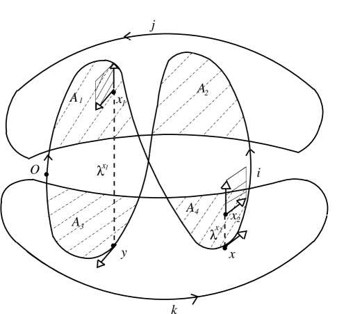
Now, observe that the integration in $x$ must be restricted to the area surrounded by curve $i$, due to the factor $F_{\Sigma_{i}x}$ in the integrand. Furthermore, for each $x$, the presence of the factor $T_{\alpha}(x,\lambda^{y})$ ensures that there will be contributions only when this point $x$ is connected through a vertical line with a point $y$ lying in the other curve $j$, in such a manner that the infinitesimal displacements along the vertical path ($dz^{\alpha}$) and along the closed curve $j$ ($dy^{\mu}$) form a non-degenerated parallelogram (see FIG. 1). Under these conditions, the contribution associated to the point $x$ is just the area of that infinitesimal parallelogram: $\epsilon^{\mu\alpha}dy^{\mu}dz^{\alpha}$.

Figure 1: Configuration with a non-vanishing $0-th$ order contribution

On the other hand, for each $x$ belonging to $\Sigma_{i}$, but not to the intersection (see $x^{,}$ in FIG. 1), there would be two contributions (more generally, an even number of them, which could be none as in the case of $x^{,,}$, shown in FIG. 1) because the parallel curves intersect twice the closed trajectory $j$. But in these cases, the net contribution of the “upper side” of curve $j$ (i.e. the piece from $A$ to $B$ in clockwise sense) plus the “down side” (the part from $B$ to $A$ in counterclockwise sense) cancel each other.

Hence, we have to sum up as many infinitesimal parallelograms as necessary to cover the area of intersection, and we recover our previous interpretation of the $0-th$ order invariant.

III.4 Interpretation of the $1-st$ order invariant $S^{(1)}$ and final remarks.

Our starting point will be expression (45) for the Yang-Mills action on-shell up to first order, expressed entirely in terms of the closed curves. Since the coefficient related to the iso-vectors $\vec{I}_{i}$ is completely antisymmetric in $i,j,k$, and these iso-vectors are arbitrary, we conclude that the following quantity is invariant:

$$Y(\gamma_{i},\gamma_{j},\gamma_{k})\equiv\ \left(\frac{1}{2\pi}\right)^{2}\left(\frac{1}{2}\,T_{[i}^{\mu x_{1}}T_{j}^{\nu x_{2}}T_{k]}^{\nu y}\ln|x-x_{1}|\ln|x-x_{2}|\partial_{\mu}\ln|x-y|\right.$$ (59)

$$\left.-T_{[i}^{\nu x\,\mu y}T_{j}^{\mu x_{1}}T_{k]}^{\nu x_{2}}\ln|y-x_{1}|\ln|x-x_{2}|\right).$$

Here, square brackets denote anti-symmetrization.

Consider the first term in (59). Making the substitution (48), and after some calculations it results

$$T_{i}^{\mu x_{1}}T_{j}^{\nu x_{2}}T_{k}^{\nu y}\ln|x-x_{1}|\ln|x-x_{2}|\partial_{\mu x}\ln|x-y|$$

$$=\epsilon^{\mu\alpha}\partial_{\alpha}F_{\Sigma_{i}x_{1}}\epsilon^{\nu\beta}\partial_{\beta}F_{\Sigma_{j}x_{2}}\epsilon^{\nu\gamma}\partial_{\gamma}F_{\Sigma_{k}y}\ln|x-x_{1}|\ln|x-x_{2}|\partial_{\mu x}\ln|x-y|$$

$$=-\epsilon^{\mu\alpha}F_{\Sigma_{i}x_{1}}F_{\Sigma_{j}x_{2}}F_{\Sigma_{k}y}\partial_{\alpha x_{1}}\ln|x-x_{1}|\partial_{\beta x_{2}}\ln|x-x_{2}|\partial_{\beta y}\partial_{\mu x}\ln|x-y|$$

$$=-(2\pi)^{3}\epsilon^{\mu\alpha}F_{\Sigma_{i}x_{1}}F_{\Sigma_{j}x_{2}}F_{\Sigma_{k}y}\partial_{\alpha x_{1}}G_{x,x_{1}}\partial_{\beta x_{2}}G_{x,x_{2}}\partial_{\beta y}\partial_{\mu x}G_{x,y}.$$ (60)

Making the substitution (56), i.e., changing to axial gauge, the last line of (III.4) can be written down as

$$-(2\pi)^{3}\epsilon^{\mu\alpha}F_{\Sigma_{i}x_{1}}F_{\Sigma_{j}x_{2}}F_{\Sigma_{k}y}T_{\alpha}(x,\lambda^{x_{1}})T_{\beta}(x,\lambda^{x_{2}})\partial_{\beta y}T_{\mu}(x,\lambda^{y}).$$ (61)

This quantity vanishes, because the straight lines $\lambda^{x}$ are parallel, which implies that the cross product of their tangent vectors is zero.

It remains to compute the second term in (59). Changing to the axial gauge by means of substitution (56), we obtain

$$Y(\gamma_{i},\gamma_{j},\gamma_{k})=-T_{i}^{\nu x,\,\mu y}\epsilon^{\mu\alpha}\epsilon^{\nu\beta}F_{\Sigma_{j}x_{1}}F_{\Sigma_{k}x_{2}}T_{\alpha}(y,\lambda^{x_{1}})T_{\beta}(x,\lambda^{x_{2}})+[ijk],$$ (62)

where $[ijk]$ means that the whole expression must be anti-symmetrized in the indices inside the bracket. This symmetry property of (62) imply that the minimal number of curves that will produce a non-trivial result is three.

To interpret this expression, let us then consider a configuration of three curves as in FIG. 2. This configuration was chosen taking into account that, as we already know, $Y(\gamma_{i},\gamma_{j},\gamma_{k})$ is meaningful whenever (46) vanishes for every pair of curves. In this configuration, the absolute values of the areas of intersection $A_{i}$, $i=1,2,3,4$ are the same, but their signs are such that the above condition is fulfilled. It should be noticed that, given the configuration of FIG. 2, only the first term in (62) contributes.

Figure 2: Example of a “linking-area” configuration detected by $Y(\gamma_{i},\gamma_{j},\gamma_{k})$

The points $x_{1}$ and $x_{2}$ must belong to the surfaces $\Sigma_{j}$ and $\Sigma_{k}$ respectively, as indicated by the surface-functions $F_{\Sigma_{j}x_{1}}$ and $F_{\Sigma_{k}x_{2}}$. Also, we have now two bundles of open straight parallel lines: the “fibers” of one of them (that corresponding to $T_{\alpha}(y,\lambda^{x_{1}})$) start at the points $y$ of $\gamma_{i}$, and end at the points $x_{1}$ of the surface surrounded by $\gamma_{j}$. The other bundle of parallel lines (corresponding to $T_{\beta}(x,\lambda^{x_{2}})$) also begins at $\gamma_{i}$, but finishes at $x_{2}$ inside $\Sigma_{k}$. As before, the contributions to expression (62) are expressed as areas of the infinitesimal parallelograms formed by vertical displacements along both the fiber and the curve where the corresponding fiber ends.

Up to this point, there is nothing specially new in the discussion of the first-order invariant. The main difference with the previous case, is due to the presence of the loop coordinate with two indices $T_{i}^{\nu x,\,\mu y}$, which introduces an intrinsic order in curve $i$ that affects which contributions must be summed up. In the integration along curve $i$ the areas of the parallelograms coming from curve $k$, which have to be multiplied by those coming from curve $j$, contribute only if the former are “created” before the later when one travels along curve $i$ starting at an arbitrary marked point ($O$, in FIG.2). Henceforth, of the four products of areas $|A_{1}||A_{4}|$, $-|A_{1}||A_{3}|$, $|A_{2}||A_{3}|$ and $-|A_{2}||A_{4}|$, that would appear if instead of $T_{i}^{\nu x,\,\mu y}$ we had $T_{i}^{\nu x}$ times $T_{i}^{\mu y}$ in (62), the last one does not contribute due to the fact that $A_{2}$ is “drawn” after $A_{4}$ was.

Then, the result of applying (62) to the picture in FIG. 2 is minus the square of the area $A_{i}^{2}$ of any of the lobules of intersection. Clearly, this is an area-preserving diffeomorphism invariant, which could not be detected by the previous order one (which in fact vanishes).

Summarizing, we have shown that classical $2d$ Yang-Mills theory coupled to non-dynamical Wong particles in Euclidean space can be used to obtain area-invariants through a perturbative scheme. This fact may be seen as an instance of a general result established in rafael , which in turn aroused as a formalization of previous results L3 ; Nudos .

The first two invariants provided by this method were explicitly computed, and a geometrically appealing interpretation was given. It is conjectured that the sequence of invariants here obtained could be seen as a kind of “projection” of the link-invariants of Milnor milnor . This and other pertinent questions will be addressed in future work.

We thank Edmundo Castillo for his assistance with the figures. This work was partially supported by Fonacit grant G2001000712.

References

- (1) E. Witten, Commun. Math. Phys. 121, 351 (1989).
- (2) J.M.F. Labastida, Chern-Simons Gauge Theory: Ten Years Later, hep-th/9905057, USC-FT-7/99, in ”Trends in Theoretical Physics II”, Buenos Aires, Argentina, 1998.
- (3) E. Guadagnini, M. Martellini and M. Mintchev, Nucl. Phys. B330, 575 (1990).
- (4) L. Leal, Mod. Phys. Lett. A 7, 541 (1992).
- (5) L. Leal, Phys. Rev. D 66, 125007 (2002); L.Leal “Knot invariants from classical field theories”, arXiv:hep-th/9911133; E. Fuenmayor, “Estudio de Representaciones Geométricas e Invariantes de Nudo en Teorías Topológicas de Calibre Acopladas con Materia”, Tesis Doctoral, UCV, 2005; E. Fuenmayor and L.Leal “High-Order Link Invariants and Classical Chern-Simons Theory”, in preparation.
- (6) R.Díaz and L.Leal, “Invariants from classical field theory”, in preparation.
- (7) S. K. Wong, Nuovo Cimento A65, 689 (1970).
- (8) M. Aganagic, H. Ooguri, N. Saulina and C. Vafa, Nucl. Phys. B 715, 304 (2005).
- (9) S. de Haro, “Chern-Simons theory, Yang-Mills, and lie algebra wanderes”, arXiv:hep-th/0412110.
- (10) X. Arsiwalla, R. Boels, M. Marino and A. Sinkovics, “Phase transitions in deformed Yang-Mills theory and topological strings”, arXiv:hep-th/0509002.
- (11) S. de Haro, “A Note on Knot Invariants and Deformed Yang-Mills”, arXiv:hep-th/0509167.
- (12) D. J. Gross and W. I. Taylor, Nucl. Phys. B 400, 181 (1993).
- (13) C. Vafa, “Two dimensional Yang-Mills, black holes and topological strings”, arXiv:hep-th/0412110.
- (14) A. M. Brzoska, F. Lenz, J. W. Negele and M. Thies, Phys. Rev. D 71, 034008 (2005).
- (15) J. Ambjorn, P. Olesen, and C. Peterson Nucl. Phys. B 240, 189 (1984).
- (16) A.P. Balachandran, M. Borchardt and A. Stern, Phys. Rev. D17, 3247 (1978).
- (17) J. Milnor, Ann. of Math. 59, 177 (1954).
- (18) C. Di Bartolo, R. Gambini, y J. Griego, Commun. Math. Phys. 158, 217 (1993).
- (19) D. Rolfsen, Knots and Links, Wilmington, Publish or Perish (1976).