Casimir effect with non-local boundary conditions

Abstract:

Non-local boundary conditions have been considered in theoretical high-energy physics with emphasis on one-loop quantum cosmology, one-loop conformal anomalies, Bose–Einstein condensation models and spectral branes. In the present paper, for the first time in the literature, the Wightman function, the vacuum expectation values of the field square and the energy-momentum tensor are investigated for a massive scalar field satisfying non-local boundary conditions on a single and two parallel plates. The vacuum forces acting on the plates are evaluated. Interestingly, suitable choices of the kernel in the non-local boundary conditions lead to forces acting on the plates that can be repulsive for intermediate distances. It is then possible to obtain a locally stable equilibrium value of the interplate distance stabilized by the vacuum forces.

1 Introduction

In recent years, non-local boundary conditions in quantum physics have been considered for at least three main purposes: (i) As part of the attempt of obtaining a consistent picture of one-loop quantum cosmology [1, 2] and in the course of investigating one-loop conformal anomalies for fermionic fields [3]. (ii) Spectral boundary conditions for Laplace-type operators on a compact manifold with boundary are partly Dirichlet, partly (oblique) Neumann conditions, where the partitioning is provided by a pseudodifferential projection; they are of interest in string and brane theory [4, 5]. (iii) As part of the investigation of bulk and surface states in Bose–Einstein condensation models [6].

In the latter case, following the work in Ref. [6], it is useful to consider a simple example given by the Laplacian acting on scalar functions on the two-dimensional plane. More precisely, given the function $q$ which is both Lebesgue summable and square-integrable on the real line, i.e. $q\in L_{1}(\mathbf{R})\cap L_{2}(\mathbf{R})$, one defines [6]

$$q_{R}(x)\equiv{\frac{1}{2\pi R}}\sum_{l=-\infty}^{\infty}e^{ilx/R}\int_{-\infty}^{\infty}e^{-ily/R}q(y)dy.$$ (1)

The function $q_{R}$ is, by construction, periodic with period $2\pi R$, and tends to $q$ as $R$ tends to $\infty$. On considering the region

$$B_{R}\equiv\left\{x,y:x^{2}+y^{2}\leq R^{2}\right\},$$ (2)

one studies the Laplacian acting on square-integrable functions on $B_{R}$, with non-local boundary conditions given by

$$\Bigr{[}u_{;N}\Bigr{]}_{\partial B_{R}}+\oint_{\partial B_{R}}q_{R}(s-s^{\prime})u(R\cos(s^{\prime}/R),R\sin(s^{\prime}/R))ds^{\prime}=0.$$ (3)

In polar coordinates, the resulting boundary-value problem reads as

$$-\left({\frac{\partial^{2}}{\partial r^{2}}}+{\frac{1}{r}}{\frac{\partial}{\partial r}}+{\frac{1}{r^{2}}}{\frac{\partial^{2}}{\partial\varphi^{2}}}\right)u=Eu,$$ (4)

$${\frac{\partial u}{\partial r}}(R,\varphi)+R\int_{-\pi}^{\pi}q_{R}(R(\varphi-\theta))u(R,\theta)d\theta=0.$$ (5)

For example, when the eigenvalue $E$ is positive in Eq. (4), the corresponding eigenfunction is

$$u_{l,E}(r,\varphi)=J_{l}(r\sqrt{E})e^{il\varphi},$$ (6)

where $J_{l}$ is the standard notation for the Bessel function of first kind of order $l\in\mathbf{Z}$. On denoting by $\widetilde{q}$ the Fourier transform of $q$, and inserting (6) into the boundary condition (5), one finds an equation leading, implicitly, to the knowledge of the positive eigenvalues, i.e.

$$\Bigr{[}\sqrt{E}J_{l}^{\prime}(R\sqrt{E})+J_{l}(R\sqrt{E}){\widetilde{q}}(l/R)\Bigr{]}=0.$$ (7)

The solutions of Eq. (7) which decay rapidly away from the boundary are the surface states, whereas the solutions which remain non-vanishing are called bulk states [6].

In the extension to gauge fields, non-local boundary conditions along the lines of Eq. (1.3) make it possible to improve the ellipticity properties of the boundary-value problem, by working with suitable symbols of the boundary operator, as shown in [7]. The price to be paid, however, is that the gauge-field and ghost operators become pseudo-differential because the gauge-fixing functional is no longer a local functional of the gauge field [7].

On the other hand, in the field-theoretical analysis of macroscopic quantum effects such as the Casimir effect, an essential point is the relation between the mode-sum energy, evaluated as the sum of zero-point energies for each normal mode, and the volume integral of the renormalized energy density. For scalar fields with general curvature coupling it has been shown that, in the discussion of this question for the Robin parallel plates geometry it is necessary to include in the energy a surface term concentrated on the boundary [8]. In subsequent work, by using variational methods, the first author of the present paper has derived an expression of the surface energy-momentum tensor for a scalar field with a general curvature coupling parameter in the general case of bulk and boundary geometries [9].

As a next step, we have been therefore led to consider the role of non-local boundary conditions in the course of studying the vacuum expectation value of the energy-momentum tensor as well as the Casimir effect itself. For this purpose, section 2 studies the Wightman function and Casimir densities for a single plate, while section 3 is devoted to vacuum densities in the region between two parallel plates. Concluding remarks are made in section 4.

2 Wightman function and Casimir densities for a single plate

We consider a real scalar field $\varphi(x)$ with general curvature coupling parameter $\zeta$ satisfying the field equation

$$\left(\nabla_{\mu}\nabla^{\mu}+m^{2}+\zeta R\right)\varphi=0,$$ (8)

where $R$ is the scalar curvature for a $(D+1)$–dimensional background spacetime, and $\nabla_{\mu}$ is the covariant derivative operator. For special cases of minimally and conformally coupled scalars one has $\zeta=0$ and $\zeta=\zeta_{c}\equiv(D-1)/4D$, respectively. Our main interest in this paper will be the Wightman function, the vacuum expectation values (VEVs) of the field square and the energy-momentum tensor induced by a single and two parallel plates in Minkowski spacetime. For this problem the background spacetime is flat and in Eq. (8) we have $R=0$. As a result the eigenmodes are independent of the curvature coupling parameter. However, the local properties of the vacuum such as energy density and vacuum stresses depend on this parameter.

In this section we consider the properties of the vacuum for the geometry of a single plate. We will use rectangular coordinates $x^{\mu}=(t,x^{1}=x,\mathbf{x}_{\parallel})$, where $\mathbf{x}_{\parallel}=(x^{2},\ldots,x^{D})$ denotes the coordinates parallel to the plate. We assume that the plate is located at $x=0$ and the field obeys a non-local boundary condition similar to Eq. (3), i.e.

$$n^{\nu}\partial_{\nu}\varphi(t,x,\mathbf{x}_{\parallel})+\int d\mathbf{x}_{\parallel}^{\prime}\,f(|\mathbf{x}_{\parallel}-\mathbf{x}_{\parallel}^{\prime}|)\varphi(t,x,\mathbf{x}_{\parallel}^{\prime})=0,\;x=0,$$ (9)

where $n^{\nu}$ is the inward-pointing normal to the boundary and the conditions on the function $f$ will be specified below. For definiteness we consider the region $x>0$ for which $n^{\nu}=\delta_{1}^{\nu}$. It can be seen that, for this type of boundary condition, the scalar product $(\varphi_{1},\varphi_{2})_{t}$ for a given spatial hypersurface $t=\mathrm{const}$, defined in the standard way (see, for instance, [10]) does not depend on the choice of hypersurface $\Sigma$. Indeed, the corresponding difference for two hypersurfaces $t=t_{1}$ and $t=t_{2}$, from the field equation, by using the Stokes theorem, reads as

$$(\varphi_{1},\varphi_{2})_{t_{2}}-(\varphi_{1},\varphi_{2})_{t_{1}}$$ (10)

$$= i\int_{t_{1}}^{t_{2}}dt\int d\mathbf{x}_{\parallel}n^{\nu}\left[\varphi_{1}^{\ast}(t,0,\mathbf{x}_{\parallel})\partial_{\nu}\varphi_{2}(t,0,\mathbf{x}_{\parallel})-\varphi_{2}(t,0,\mathbf{x}_{\parallel})\partial_{\nu}\varphi_{1}^{\ast}(t,0,\mathbf{x}_{\parallel})\right].$$

By virtue of the boundary condition (9), the integral on the right-hand side vanishes. For the standard local Robin boundary conditions, the normal derivative of the field at a given point on the boundary is determined by the value of the field at the same point. The non-local boundary condition (9) states that the normal derivative at a given point depends on the values of the field at other points on the boundary. The properties of the boundary are codified by the function $f$. In some sense, the situation here is similar to that in electrodynamics for the spatial dispersion of the dielectric permittivity, when one considers the relation between the displacement and the electric field. In electrodynamics the spatial dispersion leads to the dependence of dielectric permittivity on the wave vector. Analogously, our non-local boundary conditions lead to the dependence of the coefficient $F$ in the eigenfunctions on the wave vector ${\bf k}_{\parallel}$ (see below).

As the first stage in the investigation of local quantum effects we consider the positive-frequency Wightman function. The VEVs of the field square and the energy-momentum tensor can be obtained from the Wightman function in the coincidence limit of the arguments with an additional renormalization procedure. Instead of the Wightman function we could take any other two-point function, but we choose the Wightman function because it also determines the response of particle detectors in a given state of motion. To evaluate the positive-frequency Wightman function we use the mode-sum formula

$$\langle 0_{S}|\varphi(x^{\mu})\varphi(x^{\prime\mu})|0_{S}\rangle=\sum_{\mathbf{k}}\varphi_{\mathbf{k}}^{\ast}(x^{\mu})\varphi_{\mathbf{k}}(x^{\prime\mu}),$$ (11)

where $|0_{S}\rangle$ is the vacuum state corresponding to the geometry of a single plate. For this geometry, the normalised eigenfunctions satisfying the boundary condition (9) are given by

$$\varphi_{\mathbf{k}}(x^{\mu})=\frac{e^{i\mathbf{k}_{\parallel}\mathbf{x}_{\parallel}-i\omega t}}{\sqrt{2^{D-1}\pi^{D}\omega}}\cos(kx+\alpha),$$ (12)

where $\omega\equiv\sqrt{k^{2}+k_{\parallel}^{2}+m^{2}}$, $0\leq k<\infty$,  and the function $\alpha=\alpha(k,k_{\parallel})$ is defined by the relation

$$e^{2i\alpha}\equiv\frac{ik-F(k_{\parallel})}{ik+F(k_{\parallel})},$$ (13)

with $k_{\parallel}=|\mathbf{k}_{\parallel}|$. In the last formula we have defined the Fourier transform

$$F(k_{\parallel}) \equiv \int d\mathbf{x}_{\parallel}\,f(|\mathbf{x}_{\parallel}|)e^{i\mathbf{k}_{\parallel}\mathbf{x}_{\parallel}}$$ (14)

$$= \frac{(2\pi)^{\frac{D-1}{2}}}{k_{\parallel}^{\frac{D-3}{2}}}\int_{0}^{\infty}du\,u^{\frac{D-1}{2}}f(u)J_{\frac{D-3}{2}}(uk_{\parallel}),$$

where $J_{\nu}(x)$ is the Bessel function of first kind of order $\nu$. In the case $F(k_{\parallel})>0$ there is also a purely imaginary eigenvalue $k=iF(k_{\parallel})$ with the normalized eigenfunction

$$\varphi_{\mathbf{k}_{\parallel}}^{\mathrm{(im)}}(x^{\mu})=\sqrt{\frac{F(k_{\parallel})}{(2\pi)^{D-1}\omega^{\mathrm{(im)}}}}e^{i\mathbf{k}_{\parallel}\mathbf{x}_{\parallel}-i\omega^{\mathrm{(im)}}t-xF(k_{\parallel})},$$ (15)

and $\omega^{\mathrm{(im)}}\equiv\sqrt{k_{\parallel}^{2}+m^{2}-F^{2}(k_{\parallel})}$, $k_{\parallel}^{2}\geq F^{2}(k_{\parallel})-m^{2}$. These eigenfunctions correspond to the bound states of the quantum field. The occurrence of purely imaginary eigenvalues is proved by starting from the eigenfunctions, which depend on $x$ according to $A_{1}e^{ikx}+A_{2}e^{-ikx}$, with constants $A_{i}$. From the boundary condition one finds eventually

$$A_{1}(ik+F(k_{||}))=A_{2}(ik-F(k_{||})).$$

In addition to the solutions with both $A_{i}\not=0$, this equation has indeed solutions $A_{1}=0,ik=F(k_{||})$ and $A_{2}=0,ik=-F(k_{||})$.

To escape the instability of the vacuum state, in the discussion below we will assume that the function (14) satisfies the condition $F(k_{\parallel})\leq\sqrt{k_{\parallel}^{2}+m^{2}}$. For the convergence of the integral in (14) we need to have the behavior $f(u)=o(u^{1-D/2})$ in the limit $u\rightarrow\infty$ and the behavior $f(u)=o(u^{1-D})$ in the limit $u\rightarrow 0$, by virtue of standard summability criteria at infinity and at the origin, respectively. For the discussion below of various asymptotic cases it is useful to have the behavior of the function $F(k_{\parallel})$ for large and small values of the argument. For large values of $k_{\parallel}$, by using the asymptotic expansion of the Bessel function for large values of the argument, from (14) we see that $F(k_{\parallel})\sim o(k_{\parallel}^{\frac{3-D}{2}})$ as $k_{\parallel}\rightarrow\infty$. For small values of $k_{\parallel}$ two subcases should be distinguished. For the case of functions $f(u)\sim o(u^{1-D})$, $u\rightarrow\infty$, on using the expression for the Bessel function for small values of the argument, one finds to leading order

$$F(k_{\parallel})\approx F_{0}\equiv\frac{2\pi^{\frac{D-1}{2}}}{\Gamma\left(\frac{D-1}{2}\right)}\int_{0}^{\infty}du\,u^{D-2}f(u),\;k_{\parallel}\rightarrow 0.$$ (16)

For the functions $f(u)\sim u^{-\beta}$, $u\rightarrow\infty$, with $D/2-1<\beta<D-1$, by introducing in (14) a new integration variable $y=uk_{\parallel}$ and replacing the function $f(y/k_{\parallel})$ by its asymptotic expansion for large values of the argument, one finds $F(k_{||})\sim k_{||}^{\beta+1-D}$, $k_{||}\rightarrow 0$. In the table below we present examples of the kernel function $f$ in the boundary condition (9) with the corresponding Fourier transforms $F$. These functions depend on three parameters $f_{0}$, $x_{0}$, $\eta$.

Table 1: Examples of kernel function $f$ in the boundary condition, with Fourier transform $F$.

$f(x)$	$F(y)$
$\frac{f_{0}}{(x^{2}+x_{0}^{2})^{\frac{D-1}{2}-\eta}}$	$f_{0}\frac{2^{\eta+1}\pi^{\frac{D-1}{2}}}{\Gamma\left(\frac{D-1}{2}-\eta\right)}\left(\frac{x_{0}}{y}\right)^{\eta}K_{\eta}(x_{0}y)$
$f_{0}e^{-\eta\sqrt{x^{2}+x_{0}^{2}}}$	$(2\pi x_{0})^{\frac{D}{2}}\eta f_{0}\frac{K_{D/2}(x_{0}\sqrt{\eta^{2}+y^{2}})}{\pi\left(\eta^{2}+y^{2}\right)^{D/4}}$
$f_{0}\frac{e^{-\eta\sqrt{x^{2}+x_{0}^{2}}}}{\sqrt{x^{2}+x_{0}^{2}}}$	$2(2\pi x_{0})^{\frac{D}{2}-1}f_{0}\frac{K_{D/2-1}(x_{0}\sqrt{\eta^{2}+y^{2}})}{\left(\eta^{2}+y^{2}\right)^{D/4-1/2}}$

The positive-frequency Wightman function is obtained by substituting the eigenfunctions (12) and (15) into the mode-sum formula (11). It can be presented in the form

$$\langle 0_{S}|\varphi(x^{\mu})\varphi(x^{\prime\mu})|0_{S}\rangle=\langle 0_{M}|\varphi(x^{\mu})\varphi(x^{\prime\mu})|0_{M}\rangle$$ (17)

$$+\int\frac{d\mathbf{k}_{\parallel}}{(2\pi)^{D}}e^{i\mathbf{k}_{\parallel}(\mathbf{x}_{\parallel}-\mathbf{x}_{\parallel}^{\prime})}\int_{0}^{\infty}dk\frac{e^{i\omega(t^{\prime}-t)}}{\omega}\cos\left[k(x+x^{\prime})+2\alpha\right]$$

$$+\int\frac{d\mathbf{k}_{\parallel}}{(2\pi)^{D-1}}\frac{F(k_{\parallel})}{\omega^{\mathrm{(im)}}}\theta(F(k_{\parallel}))e^{i\mathbf{k}_{\parallel}(\mathbf{x}_{\parallel}-\mathbf{x}_{\parallel}^{\prime})-(x+x^{\prime})F(k_{\parallel})+i(t^{\prime}-t)\omega^{\mathrm{(im)}}},$$

where $|0_{M}\rangle$ stands for the vacuum state in Minkowski spacetime without boundary, with $\langle 0_{M}|\varphi(x^{\mu})\varphi(x^{\prime\mu})|0_{M}\rangle$ the corresponding Wightman function, and $\theta$ is the Heaviside step function. The last term on the right of this formula is the contribution of bound states. Note that, by using the definition for $\alpha$, the $\cos$ function in the integrand can be also presented in the form

$$\cos\left(ky+2\alpha\right)=\frac{k^{2}-F^{2}(k_{\parallel})}{k^{2}+F^{2}(k_{\parallel})}\cos ky-\frac{2kF(k_{\parallel})}{k^{2}+F^{2}(k_{\parallel})}\sin ky.$$ (18)

The integrals in (17) over the angular part of the vector ${\mathbf{k}}_{\parallel}$ can be explicitly evaluated with the help of the formula already used in (14). In the coincidence limit from formula (17) one finds the VEV of the field square

$$\langle 0_{S}|\varphi^{2}|0_{S}\rangle = \langle 0_{M}|\varphi^{2}|0_{M}\rangle+\frac{S_{D-1}}{(2\pi)^{D}}\int_{0}^{\infty}dk_{\parallel}\,k_{\parallel}^{D-2}\int_{0}^{\infty}dk\frac{\cos\left(2kx+2\alpha\right)}{\omega}$$ (19)

$$+\frac{S_{D-1}}{(2\pi)^{D-1}}\int dk_{\parallel}\,k_{\parallel}^{D-2}\frac{F(k_{\parallel})}{\omega^{\mathrm{(im)}}}\theta(F(k_{\parallel}))e^{-2xF(k_{\parallel})},$$

where $S_{D-1}=2\pi^{(D-1)/2}/\Gamma((D-1)/2)$ is the surface area of the unit sphere in $D$-dimensional space. The last two terms on the right of this formula are induced by the plate. For points away from the boundary ($x\neq 0$) these terms are finite and the divergences in the VEV of the field square are contained in the first term only. Hence, here the renormalization procedure is the same as that for Minkowski spacetime without boundary.

To obtain an alternative form for the VEV of the field square, we write the $\cos$ function in the second term on the right of (19) in terms of the exponential functions and rotate the integration contour in the complex $k$-plane by the angle $\pi/2$ for the term with $e^{2ikx}$ and by the angle $-\pi/2$ for the term with $e^{-2ikx}$. We assume that the points $\pm i\sqrt{k_{\parallel}^{2}+m^{2}}$ and the poles $\pm iF(k_{\parallel})$ in the case $F(k_{\parallel})>0$ are bypassed on the right by semicircles with small radii. In such a way the following relation is obtained:

$$\int_{0}^{\infty}dk\frac{\cos\left(2kx+2\alpha\right)}{\omega} = \int_{\sqrt{k_{\parallel}^{2}+m^{2}}}^{\infty}du\,\frac{e^{-2ux}}{\sqrt{u^{2}-k_{\parallel}^{2}-m^{2}}}\frac{u+F(k_{\parallel})}{u-F(k_{\parallel})}$$ (20)

$$-2\pi F(k_{\parallel})\frac{e^{-2xF(k_{\parallel})}\theta(F(k_{\parallel}))}{\sqrt{k_{\parallel}^{2}+m^{2}-F^{2}(k_{\parallel})}}.$$

Now we see that the second term on the right of this formula cancels out the third term on the right-hand side of formula (19) and we obtain

$$\langle\varphi^{2}\rangle_{\mathrm{sub}} = \langle 0_{S}|\varphi^{2}|0_{S}\rangle-\langle 0_{M}|\varphi^{2}|0_{M}\rangle=\frac{S_{D-1}}{(2\pi)^{D}}\int_{0}^{\infty}dk_{\parallel}\,k_{\parallel}^{D-2}$$ (21)

$$\times\int_{\sqrt{k_{\parallel}^{2}+m^{2}}}^{\infty}du\,\frac{e^{-2ux}}{\sqrt{u^{2}-k_{\parallel}^{2}-m^{2}}}\frac{u+F(k_{\parallel})}{u-F(k_{\parallel})}.$$

The VEVs of the field square in the cases of Dirichlet and Neumann boundary conditions are obtained from the general formula (21) in the limits $F(k_{\parallel})\rightarrow\infty$ and $F(k_{\parallel})\rightarrow 0$, respectively. In these cases the integrals are evaluated by introducing a new integration variable $v\equiv\sqrt{u^{2}-k_{\parallel}^{2}-m^{2}}$ and passing to polar coordinates in the $(k_{\parallel},v)$-plane. This simple calculation leads to the result

$$\left(\langle\varphi^{2}\rangle_{\mathrm{sub}}\right)_{\mathrm{Dirichlet}}=-\left(\langle\varphi^{2}\rangle_{\mathrm{sub}}\right)_{\mathrm{Neumann}}=-\frac{(m/x)^{\frac{D-1}{2}}}{2^{D}\pi^{\frac{D+1}{2}}}K_{(D-1)/2}(2mx),$$ (22)

where $K_{\nu}(x)$ is the modified Bessel function of second kind. The VEV of the field square induced by a single plate on the background spacetime $R^{(D,1)}\times\Sigma$, with an internal space $\Sigma$ and local Robin boundary condition, is investigated in [11] as a limiting case of the braneworld geometry.

Having the Wightman function (17) and the VEV of the field square we can evaluate the VEV of the energy-momentum tensor by making use of the formula

$$\langle 0_{S}|T_{\mu\nu}|0_{S}\rangle=\lim_{x^{\prime}\rightarrow x}\langle 0_{S}|\partial_{\mu}\varphi(x^{\alpha})\partial_{\nu}^{\prime}\varphi(x^{\prime\alpha})|0_{S}\rangle+\left[\left(\zeta-\frac{1}{4}\right)g_{\mu\nu}\partial_{\alpha}\partial^{\alpha}-\zeta\partial_{\mu}\partial_{\nu}\right]\langle 0_{S}|\varphi^{2}|0_{S}\rangle.$$ (23)

With the help of formulae (17) and (21) for the boundary induced part the following result is obtained (no summation over $\nu$):

$$\langle T_{\mu}^{\nu}\rangle_{\mathrm{sub}} = \langle 0_{S}|T_{\mu}^{\nu}|0_{S}\rangle-\langle 0_{M}|T_{\mu}^{\nu}|0_{M}\rangle=\frac{S_{D-1}\delta_{\mu}^{\nu}}{(2\pi)^{D}}\int_{0}^{\infty}dk_{\parallel}\,k_{\parallel}^{D-2}$$ (24)

$$\times\int_{\sqrt{k_{\parallel}^{2}+m^{2}}}^{\infty}du\,\frac{A_{\nu}(u,k_{\parallel})e^{-2ux}}{\sqrt{u^{2}-k_{\parallel}^{2}-m^{2}}}\frac{u+F(k_{\parallel})}{u-F(k_{\parallel})},$$

where we have introduced the notations

$$A_{0}(u,k_{\parallel}) \equiv k_{\parallel}^{2}+m^{2}-4\zeta u^{2},\;A_{1}(u,k_{\parallel})=0,$$ (25)

$$A_{\nu}(u,k_{\parallel}) \equiv (1-4\zeta)u^{2}-\frac{k_{\parallel}^{2}}{(D-1)},\;\nu=2,\ldots,D.$$ (26)

For the evaluation of the $T_{\nu}^{\nu}$ components, with $\nu=2,3,...$, we note that, from the problem symmetry, one has $T_{2}^{2}=T_{3}^{3}=...$ and hence

$$T_{2}^{2}=\sum_{\nu=2}^{D}{T_{\nu}^{\nu}\over(D-1)}.$$

For the sum in the last formula, the integrand contains the factor

$$\sum_{\nu=2}^{D}T_{\nu}^{\nu}\rightarrow-k_{||}^{2}+u^{2}(1-4\zeta)(D-1).$$

As we see, the vacuum stress in the direction perpendicular to the plate, $\langle T_{1}^{1}\rangle_{\mathrm{sub}}$, vanishes. This result could be also directly obtained from the continuity equation $\partial_{\nu}\langle T_{\mu}^{\nu}\rangle_{\mathrm{sub}}=0$ for the boundary induced VEV of the energy-momentum tensor. It can be checked that the tensor (24) is traceless for a conformally coupled massless scalar field. In the case of the local boundary condition of Robin type the function $F(k_{\parallel})$ is a constant and the expression for the corresponding energy-momentum tensor is further simplified by introducing a new integration variable $v\equiv\sqrt{u^{2}-k_{\parallel}^{2}-m^{2}}$ and passing to polar coordinates in the $(k_{\parallel},v)$-plane as before (2.15). In particular, for the massless case we obtain the result given in [8]. Note that in this case the VEV of the energy-momentum tensor vanishes for a conformally coupled scalar field. For the non-local boundary condition, in general, this is not the case. Another important difference is that, unlike the local case, for non-local boundary conditions, in general, $\langle T_{0}^{0}\rangle_{\mathrm{sub}}\neq\langle T_{\mu}^{\mu}\rangle_{\mathrm{sub}}$ (no summation over $\mu=2,\ldots,D$). For Dirichlet and Neumann boundary conditions the vacuum energy-momentum tensor is further simplified by a method similar to that used for the VEV of the field square, and one finds (no summation over $\mu$)

$$\left(\langle T_{\mu}^{\mu}\rangle_{\mathrm{sub}}\right)_{\mathrm{Dirichlet}}=-\left(\langle T_{\mu}^{\mu}\rangle_{\mathrm{sub}}\right)_{\mathrm{Neumann}}$$ (27)

$$= \frac{(m/x)^{\frac{D+1}{2}}}{2^{D}\pi^{\frac{D+1}{2}}}\left[2D(\zeta-\zeta_{c})K_{\frac{D+1}{2}}(2mx)+(4\zeta-1)mxK_{\frac{D-1}{2}}(2mx)\right],$$

$\mu=0,2,\ldots,D$. In the Dirichlet case the corresponding energy density is negative everywhere for both minimally and conformally coupled scalars. The vacuum energy-momentum tensor for a plate on the background spacetime $R^{(D,1)}\times\Sigma$, with an internal space $\Sigma$ and local Robin boundary condition is investigated in [16].

Now let us consider the limiting cases of the VEVs (21), (24). These VEVs diverge on the boundary. Surface divergences are well-known in quantum field theory with boundaries and are investigated for various types of boundary geometries and boundary conditions (see, for instance, [10, 12]). They result from the idealization of the boundaries as perfectly smooth surfaces which are perfect reflectors at all frequencies. It seems plausible that such effects as surface roughness, or the microstructure of the boundary on small scales can introduce a physical cutoff needed to produce finite values of surface quantities. An alternative mechanism for introducing a cutoff which removes singular behaviour on boundaries is to allow the position of the boundary to undergo quantum fluctuations [13]. Such fluctuations smear out the contribution of the high-frequency modes without the need to introduce an explicit high-frequency cutoff. Note that in this paper we consider boundary induced vacuum densities which are finite away from the boundary. We expect that similar results would be obtained in the model where instead of externally imposed boundary condition the fluctuating field is coupled to a smooth background potential that implements the boundary condition in a certain limit [14]. In the problem under consideration, for the points near the plate, the main contribution results from large values of $u$. To leading order we can omit $F(k_{\parallel})$ in the integrands and the VEVs behave as those for the Neumann boundary conditions, i.e.

$$\langle\varphi^{2}\rangle_{\mathrm{sub}}\approx\frac{x^{1-D}}{\left(4\pi\right)^{\frac{D+1}{2}}}\Gamma\left(\frac{D-1}{2}\right),\quad\langle T_{\mu}^{\mu}\rangle_{\mathrm{sub}}\approx\frac{2D(\zeta_{c}-\zeta)}{\left(4\pi\right)^{\frac{D+1}{2}}x^{D+1}}\Gamma\left(\frac{D+1}{2}\right).$$ (28)

For large distances from the plate the main contribution to the VEVs comes from small values of $u$. It can be seen that, for a massless field or for a massive field with $f(u)\sim u^{-\beta}$, $D/2-1<\beta<D-1$, at large distances the VEVs behave as those for Dirichlet boundary condition. For the case of massive field with $f(u)\sim o(u^{1-D})$, to leading order one has

$$\langle\varphi^{2}\rangle_{\mathrm{sub}}\approx\frac{F_{0}+m}{F_{0}-m}\left(\langle\varphi^{2}\rangle_{\mathrm{sub}}\right)_{\mathrm{Dirichlet}},\;x\rightarrow\infty,$$ (29)

and a similar relation for the VEV of the energy-momentum tensor. Here $F_{0}$ is defined by relation (16).

We have done numerical calculations for the components of the vacuum energy-momentum tensor by taking, for example, the kernel function

$$f(x)\equiv f_{0}e^{-\eta x}.$$ (30)

The corresponding Fourier transform $F(k_{\parallel})$ is obtained from the second line of the table given earlier in the limit $x_{0}\rightarrow 0$, i.e.

$$F(k_{\parallel})=\frac{\eta F_{1}}{\left(1+k_{\parallel}^{2}/\eta^{2}\right)^{D/2}},$$ (31)

with the notation $F_{1}\equiv 2^{D-1}\pi^{\frac{D}{2}-1}\Gamma(D/2)f_{0}/\eta^{D}$. In figure 1 we have presented the vacuum energy density (full curves) and ${T}_{2}^{2}$-stress (dashed curves) as functions on $\eta x$ for various values of the parameter $F_{1}$ (numbers near the curves) for a minimally coupled $D=3$ scalar field. The energy density is positive for the region near the plate and is negative at large distances from the plate, having the negative minimum for some intermediate distance. The corresponding curves for the energy density of the conformally coupled scalar field are presented in figure 2. In this case the ${T}_{2}^{2}$-stress is related to the energy density by the traceless condition: $\langle T_{2}^{2}\rangle_{\mathrm{sub}}=-\langle T_{0}^{0}\rangle_{\mathrm{sub}}/2$. Note that, for the case of a conformally coupled massless scalar field with local boundary condition, the corresponding vacuum energy-momentum tensor vanishes.

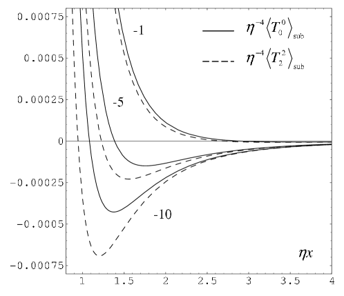
Figure 1: Single-plate induced vacuum densities $\langle T_{0}^{0}\rangle_{\mathrm{sub}}/\eta^{D+1}$ (full curves) and $\langle T_{2}^{2}\rangle_{\mathrm{sub}}/\eta^{D+1}$ (dashed curves) as functions of $\eta x$ for a minimally coupled massless scalar in $D=3$ in the case of kernel function (30). The numbers near the curves are the values of the parameter $F_{1}$ defined in the paragraph after formula (31).

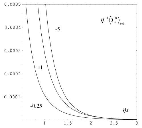
Figure 2: Single-plate induced vacuum energy density $\langle T_{0}^{0}\rangle_{\mathrm{sub}}/\eta^{D+1}$ as a function of $\eta x$ for a conformally coupled massless scalar in $D=3$ in the case of kernel function (30). The numbers near the curves are the values of the parameter $F_{1}$ defined in the paragraph after formula (31). The vacuum stress $\langle T_{2}^{2}\rangle_{\mathrm{sub}}$ is expressed through the energy density by the traceless condition.

3 Vacuum densities in the region between two parallel plates

3.1 Eigenfunctions

In this section we investigate the VEVs for the geometry of two parallel plates. We assume that the plates are located at $x=a_{j}$, $j=1,2$ and the field obeys non-local boundary conditions

$$n_{(j)}^{\nu}\partial_{\nu}\varphi(x^{\mu})+\int d\mathbf{x}_{\parallel}^{\prime}\,f_{j}(|\mathbf{x}_{\parallel}-\mathbf{x}_{\parallel}^{\prime}|)\varphi(x^{\prime\mu})=0,\;x=a_{j},$$ (32)

where $n_{(j)}^{\nu}$ is the inward-pointing unit normal to the boundary at $x=a_{j}$. Here we consider the general case when the kernel functions $f_{j}$ determining the properties of the boundaries are different for the plates. The VEVs in the regions $x<a_{1}$ and $x>a_{2}$ coincide with the corresponding quantities for a single plate geometry and are investigated in the previous section. Here we consider the region between the plates with $n_{(j)}^{\nu}=(-1)^{j-1}\delta_{1}^{\nu}$. In this region the corresponding eigenfunctions are presented in two equivalent forms corresponding to $j=1,2$, i.e.

$$\varphi_{\mathbf{k}}(x^{\mu})=\beta(k,k_{\parallel})e^{i\mathbf{k}_{\parallel}\mathbf{x}_{\parallel}-i\omega t}\cos\left[k|x-a_{j}|+\alpha_{j}\right],$$ (33)

where $\alpha_{j}=\alpha_{j}(k,k_{\parallel})$ is defined by the relation

$$e^{2i\alpha_{j}(k,k_{\parallel})}\equiv\frac{ik-(-1)^{j-1}F_{j}(k_{\parallel})}{ik+(-1)^{j-1}F_{j}(k_{\parallel})},$$ (34)

with the definition of Fourier transform $F_{j}(k_{||})$ similar to Eq. (14), i.e.

$$F_{j}(k_{\parallel}) \equiv \int d\mathbf{x}_{\parallel}\,f_{j}(|\mathbf{x}_{\parallel}|)e^{i\mathbf{k}_{\parallel}\mathbf{x}_{\parallel}}$$ (35)

$$= \frac{(2\pi)^{\frac{D-1}{2}}}{k_{\parallel}^{\frac{D-3}{2}}}\int_{0}^{\infty}du\,u^{\frac{D-1}{2}}f_{j}(u)J_{\frac{D-3}{2}}(uk_{\parallel}).$$

The corresponding eigenvalues $z=ka$, $a=a_{2}-a_{1}$, are solutions of the following transcendental equation:

$$\left(z^{2}-c_{1}c_{2}\right)\sin z+\left(c_{1}+c_{2}\right)z\cos z=0,$$ (36)

where the coefficients $c_{j}$ are defined by the relations

$$c_{j}\equiv(-1)^{j-1}aF_{j}(k_{\parallel}).$$ (37)

Equation (36) is obtained by bearing in mind that the $x$-dependence in the eigenfunctions has the form $A_{1}e^{ikx}+A_{2}e^{-ikx}$. The boundary conditions (32) lead therefore to the linear homogeneous system

$$(F_{1}+ik)e^{ika_{1}}A_{1}+(F_{1}-ik)e^{-ika_{1}}A_{2}=0,$$ (38)

$$(F_{2}+ik)e^{ika_{2}}A_{1}+(F_{2}-ik)e^{-ika_{2}}A_{2}=0.$$ (39)

Non-trivial solutions for $A_{1}$ and $A_{2}$ exist if and only if Eq. (36) holds. The expression for the coefficient $\beta(k,k_{\parallel})$ in (33) is obtained from the normalization condition:

$$\beta^{-2}(ka,k_{\parallel})=(2\pi)^{D-1}a\omega\left[1+\frac{\sin(ka)}{ka}\cos(ka+2\alpha_{j})\right].$$ (40)

The eigenvalue condition (36) has an infinite set of real zeros which we will denote by $z=\lambda_{n}$, $n=1,2,\ldots$. In addition, depending on the values of the coefficients $c_{j}$, this equation has two or four complex conjugate purely imaginary zeros (see, for instance, [8]) $\pm iy_{l}$, $y_{l}>0$.

3.2 Wightman function

Substituting the eigenfunctions (33) into the corresponding mode-sum formula, for the positive-frequency Wightman function in the region between two plates one finds

$$\langle 0|\varphi(x^{\mu})\varphi(x^{\prime\mu})|0\rangle=\int d\mathbf{k}_{\parallel}e^{i\mathbf{k}_{\parallel}(\mathbf{x}_{\parallel}-\mathbf{x}_{\parallel}^{\prime})}\sum_{z=\lambda_{n},iy_{l}}\frac{e^{i\omega(t^{\prime}-t)}}{\beta^{2}(z,k_{\parallel})}\cos(zx_{j}+\alpha_{j})\cos(zx_{j}^{\prime}+\alpha_{j}),$$ (41)

where $|0\rangle$ is the vacuum state in the region between the plates and we use the notations

$$x_{j}\equiv\frac{|x-a_{j}|}{a},\;x_{j}^{\prime}\equiv\frac{|x^{\prime}-a_{j}|}{a}.$$ (42)

The summation over the eigenvalues $\lambda_{n}$, $iy_{l}$ can be done by using the formula

$$\sum_{z=\lambda_{n},iy_{l}}\frac{h(z)}{1+\cos(z+2\alpha_{1})\sin z/z} = -\frac{1}{2}\frac{h(0)}{1-c_{1}^{-1}-c_{2}^{-1}}+\frac{1}{\pi}\int_{0}^{\infty}dzh(z)$$ (43)

$$+\frac{i}{\pi}\int_{0}^{\infty}dt\frac{h(te^{\pi i/2})-h(te^{-\pi i/2})}{\frac{(t-c_{1})(t-c_{2})}{(t+c_{1})(t+c_{2})}e^{2t}-1}$$

$$-\frac{\pi\theta(c_{j})}{2c_{j}}\left[g_{j}(c_{j}e^{\pi i/2})+g_{j}(c_{j}e^{-\pi i/2})\right],$$

where

$$g_{j}(z)\equiv\left(z^{2}+c_{j}^{2}\right)h(z).$$ (44)

Formula (43) is derived in [8] as a special case of the generalized Abel–Plana summation formula [15]. As a function $h$ (with first-order poles at $z=\pm ic_{j}$) we take

$$h(z)\equiv\frac{e^{i\omega(t^{\prime}-t)}}{a\omega}\cos(zx_{j}+\alpha_{j})\cos(zx_{j}^{\prime}+\alpha_{j}),\;\omega\equiv\sqrt{z^{2}/a^{2}+k_{\parallel}^{2}+m^{2}},$$ (45)

where the function $\alpha_{j}=\alpha_{j}(z/a,k_{\parallel})$ is defined by formula (34). By using the relation (from Eq. (18))

$$\cos(y+2\alpha_{j})=\frac{z^{2}-c_{j}^{2}}{z^{2}+c_{j}^{2}}\cos y-\frac{2zc_{j}}{z^{2}+c_{j}^{2}}\sin y,$$ (46)

it can be seen that

$$g_{j}(c_{j}e^{\pi i/2})+g_{j}(c_{j}e^{-\pi i/2})=2c_{j}^{2}\frac{e^{i\omega^{\mathrm{(im)}}(t^{\prime}-t)}}{a\omega^{\mathrm{(im)}}}e^{-c_{j}(x_{j}+x_{j}^{\prime})}.$$ (47)

Moreover, by making use of the definition for $\alpha_{j}$ we see that $e^{2i\alpha_{j}(0,k_{\parallel})}=-1$, and hence $\cos(2\alpha_{j}(0,k_{\parallel}))=-1$. This implies in turn that $h(0)=0$. The resulting Wightman function from (41) is found to be

$$\langle 0|\varphi(x^{\mu})\varphi(x^{\prime\mu})|0\rangle = \langle 0_{S}|\varphi(x^{\mu})\varphi(x^{\prime\mu})|0_{S}\rangle_{j}+\frac{4}{(2\pi)^{D}}\int d\mathbf{k}_{\parallel}e^{i\mathbf{k}_{\parallel}(\mathbf{x}_{\parallel}-\mathbf{x}_{\parallel}^{\prime})}$$ (48)

$$\times\int_{a\sqrt{k_{\parallel}^{2}+m^{2}}}^{\infty}dt\frac{\cosh(tx_{j}+\tilde{\alpha}_{j})\cosh(tx_{j}^{\prime}+\tilde{\alpha}_{j})}{\frac{(t-c_{1})(t-c_{2})}{(t+c_{1})(t+c_{2})}e^{2t}-1}$$

$$\times\frac{\cosh\left[(t-t^{\prime})\sqrt{t^{2}/a^{2}-k_{\parallel}^{2}-m^{2}}\right]}{\sqrt{t^{2}-k_{\parallel}^{2}a^{2}-m^{2}a^{2}}},$$

where the function $\tilde{\alpha}_{j}=\tilde{\alpha}_{j}(t,k_{\parallel})$ is defined by the relation

$$e^{2\tilde{\alpha}_{j}}\equiv\frac{t-c_{j}}{t+c_{j}},$$ (49)

and $\langle 0_{S}|\varphi(x^{\mu})\varphi(x^{\prime\mu})|0_{S}\rangle_{j}$ is the Wightman function for a single plate located at $x=a_{j}$. On taking the coincidence limit, for the VEV of the field square we obtain the formula

$$\langle 0|\varphi^{2}|0\rangle = \langle 0_{S}|\varphi^{2}|0_{S}\rangle_{j}+\frac{4S_{D-1}}{(2\pi)^{D}}\int_{0}^{\infty}dk_{\parallel}k_{\parallel}^{D-2}\int_{a\sqrt{k_{\parallel}^{2}+m^{2}}}^{\infty}dt\frac{\cosh^{2}(tx_{j}+\tilde{\alpha}_{j})}{\sqrt{t^{2}-k_{\parallel}^{2}a^{2}-m^{2}a^{2}}}$$ (50)

$$\times\left[\frac{(t-c_{1})(t-c_{2})}{(t+c_{1})(t+c_{2})}e^{2t}-1\right]^{-1},$$

where $\langle 0_{S}|\varphi^{2}|0_{S}\rangle_{j}$ is the corresponding VEV for the geometry of a single plate at $x=a_{j}$ and is investigated in the previous section. The surface divergences on the plate at $x=a_{j}$ are contained in this term. The second term on the right of formula (50) is finite at $x=a_{j}$ and is induced by the second plate located at $x=a_{j_{1}}$, $j_{1}=1,2$, $j_{1}\neq j$. This term diverges at $x=a_{j_{1}}$. The corresponding divergence is the same as that for the geometry of a single plate located at $x=a_{j_{1}}$.

3.3 VEV of the energy-momentum tensor and vacuum forces

The vacuum expectation value of the energy-momentum tensor is evaluated by formula (23) with the vacuum state $|0\rangle$. By taking into account formulae (48), (50), for the region between the plates one finds (no summation over $\nu$)

$$\langle 0|T_{\mu}^{\nu}|0\rangle = \langle 0_{S}|T_{\mu}^{\nu}|0_{S}\rangle_{j}+\delta_{\mu}^{\nu}\frac{2S_{D-1}}{(2\pi)^{D}}\int_{0}^{\infty}dk_{\parallel}k_{\parallel}^{D-2}\int_{a\sqrt{k_{\parallel}^{2}+m^{2}}}^{\infty}\frac{f_{j\nu}(t,k_{\parallel},x)dt}{\sqrt{t^{2}-k_{\parallel}^{2}a^{2}-m^{2}a^{2}}}$$ (51)

$$\times\left[\frac{(t-c_{1})(t-c_{2})}{(t+c_{1})(t+c_{2})}e^{2t}-1\right]^{-1},$$

where $\langle 0_{S}|T_{\mu}^{\nu}|0_{S}\rangle_{j}$ is the vacuum energy-momentum tensor for the geometry of a single plate located at $x=a_{j}$, and the second term on the right is the part of the energy-momentum tensor induced by the presence of the second plate. In formula (51) we have defined

$$f_{j0}(t,k_{\parallel},x) \equiv k_{\parallel}^{2}+m^{2}-t^{2}/a^{2}+\left(k_{\parallel}^{2}+m^{2}-4\zeta t^{2}/a^{2}\right)\cosh\left(2tx_{j}+2\tilde{\alpha}_{j}\right),$$ (52)

$$f_{j1}(t,k_{\parallel},x) \equiv t^{2}/a^{2},$$ (53)

$$f_{j\nu}(t,k_{\parallel},x) \equiv -\frac{k_{\parallel}^{2}}{(D-1)}-\left[\frac{k_{\parallel}^{2}}{(D-1)}+(4\zeta-1)\frac{t^{2}}{a^{2}}\right]\cosh\left(2tx_{j}+2\tilde{\alpha}_{j}\right),$$ (54)

with $\nu=2,3,\ldots,D$. It can be easily checked that the vacuum energy-momentum tensor is traceless for a conformally coupled massless scalar field. As we could expect from the problem symmetry, the vacuum stresses in the directions parallel to the plates are isotropic. Note that the $T_{1}^{1}$-component of the energy-momentum tensor is uniform. This also follows from the continuity equation for the VEV of the energy-momentum tensor. In particular, the $T_{1}^{1}$-stress is finite on the plates and determines the vacuum force acting per unit surface of the plate:

$$p = -\langle 0|T_{1}^{1}|0\rangle=-\frac{2S_{D-1}}{(2\pi)^{D}}\int_{0}^{\infty}du\,u^{D-2}\int_{\sqrt{u^{2}+m^{2}}}^{\infty}\frac{t^{2}dt}{\sqrt{t^{2}-u^{2}-m^{2}}}$$ (55)

$$\times\left[\frac{(t-F_{1}(u))(t+F_{2}(u))}{(t+F_{1}(u))(t-F_{2}(u))}e^{2at}-1\right]^{-1}.$$

When the functions $F_{j}(u)=\mathrm{const}$, this formula can be simplified by introducing a new integration variable $v\equiv\sqrt{t^{2}-u^{2}-m^{2}}$ and passing to polar coordinates in the $(u,v)$ plane. After integrating over the angular part one finds the formula

$$p=-\frac{2^{1-D}\pi^{-D/2}}{\Gamma(D/2)}\int_{m}^{\infty}dt\frac{t^{2}\left(t^{2}-m^{2}\right)^{\frac{D}{2}-1}}{\frac{(t-F_{1})(t+F_{2})}{(t+F_{1})(t-F_{2})}e^{2at}-1}.$$ (56)

For a massless scalar field this result coincides with the formula obtained in [8]. The VEVs of the field square and the energy-momentum tensor for the geometry of two parallel plates on the background spacetime $R^{(D_{1},1)}\times\Sigma$ with an internal space $\Sigma$ and local Robin boundary conditions are investigated in [11, 16]. The vacuum forces for Dirichlet and Neumann boundary conditions are the same and are obtained from (56) as special cases with $F_{j}=\infty$ and $F_{j}=0$, respectively. These forces are attractive for all interplate distances.

Now we turn to the discussion of the general formula (55) for the vacuum forces in the limiting cases corresponding to small and large interplate distances. For this it is convenient to introduce a new integration variable $v\equiv\sqrt{t^{2}-u^{2}-m^{2}}$ as above and to pass to polar coordinates $(r,\theta)$ in the $(u,v)$ plane. For small distances the main contribution to the $r$-integral comes from large values of $r$. From the asymptotic behavior of the functions $F_{j}(u)$ for large values of the argument described in section 2, the functions $F_{j}(u)$ in the coefficient of $e^{2at}$ may be omitted and, to leading order, the corresponding forces coincide with the vacuum forces in the case of Neumann boundary conditions and are attractive. For large distance between the plates the main contribution to the integral results from small values of $r$ and two subcases should be distinguished. For a massless scalar field or for a massive field with kernel functions $f_{j}(u)\sim u^{-\beta_{j}}$, $D/2-1<\beta_{j}<D-1$, $u\rightarrow\infty$, the terms with $t$ in the coefficient of $e^{2at}$ may be omitted and the vacuum forces coincide with those for the Dirichlet case and are attractive. In the second subcase, corresponding to the kernel functions $f_{j}(u)\sim o(u^{1-D})$, $u\rightarrow\infty$, to leading order the vacuum forces are given by expressions which are obtained from (55) by the replacements $t\pm F_{j}(u)\rightarrow m\pm F_{j0}$ in the coefficient of $e^{2at}$, where the constants $F_{j0}$ are defined by formulae similar to (16) with the replacements $f(u)\rightarrow f_{j}(u)$.

We have evaluated numerically the vacuum forces acting on the plates in the case of the kernel functions

$$f_{j}(x)\equiv f_{0j}e^{-\eta_{j}x}.$$ (57)

The corresponding Fourier transforms $F_{j}(k_{\parallel})$ are given by formulae obtained from Eq. (31) by the replacements $F_{1}\rightarrow F_{1}^{(j)}$, $\eta\rightarrow\eta_{j}$. The parameters $F_{1}^{(j)}$ are defined by the formulae obtained from the corresponding expression for $F_{1}$ in the paragraph after formula (31) by the replacements $\eta\rightarrow\eta_{j}$, $f_{0}\rightarrow f_{0j}$. In figure 3 we have plotted the vacuum pressure on the plate as a function on $\eta a$ for a massless scalar in $D=3$ in the case of the kernel functions (57) with $\eta_{1}=\eta_{2}\equiv\eta$ and $F_{1}^{(2)}=10$. The numbers near the curves are the values of the parameter $F_{1}^{(1)}$. For the values $F_{1}^{(1)}\lesssim-1.08$ the vacuum pressure is negative for all interplate distances and the corresponding vacuum forces are attractive. For the values $F_{1}^{(1)}>-1.08$ there are two values of the distance between the plates for which the vacuum forces vanish. These values correspond to equilibrium positions of the plates. For the values of the distance in the region between these positions the vacuum forces acting on plates are repulsive. Thus, the left equilibrium position is unstable and the right one is locally stable.

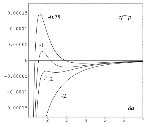
Figure 3: Vacuum pressure on the plate, $p/\eta^{D+1}$, as a function of $\eta a$ for a massless scalar in $D=3$ in the case of the kernel functions (57) with $\eta_{1}=\eta_{2}$ and $F_{1}^{(2)}=10$. The numbers near the curves are the values of the parameter $F_{1}^{(1)}$ defined in the paragraph after formula (31).

4 Concluding remarks

In this paper we have investigated the positive-frequency Wightman function, the VEVs of the field square and the energy-momentum tensor for a scalar field with non-local boundary conditions on a single and two parallel plates in Minkowski spacetime. For the case of a single plate geometry we have considered the boundary condition of the form (9), where the kernel function $f(x_{\parallel})$ describes the properties of the boundary. The VEVs of the physical quantities bilinear in the field are determined by the Fourier transform $F(k_{\parallel})$ of this function. By evaluating the corresponding mode-sum, we have presented the Wightman function as the sum of a Minkowskian part without boundary and boundary induced parts, formula (17). The last term in this formula corresponds to the contribution of bound states. The boundary induced part in the VEV of the field square is obtained in the coincidence limit of the arguments of the Wightman function and is given by formula (21). The VEV of the energy-momentum tensor is obtained by acting with the corresponding second-order differential operator on the Wightman function and taking the coincidence limit. This VEV is determined by formula (24). The vacuum stress in the direction orthogonal to the plate vanishes, and hence the corresponding vacuum force is zero.

Unlike the case of local boundary conditions, in the non-local case the vacuum energy-momentum tensor does not vanish for a conformally coupled massless scalar field. Another important difference is that for non-local boundary conditions, in general, $\langle T_{0}^{0}\rangle_{\mathrm{sub}}\neq\langle T_{\mu}^{\mu}\rangle_{\mathrm{sub}}$, $\mu=2,\ldots,D$.

As in the case of local boundary conditions, the energy density and the vacuum stresses diverge on the surface of the plate. For a nonconformally coupled scalar field the leading term in the corresponding asymptotic expansion is the same as that for Neumann boundary condition. As an example, in figures 1 and 2 we have plotted the vacuum energy density and the vacuum stress as functions of the distance from the plate for a choice of kernel function $f$ given by (30).

In section 3 we have considered the geometry of two parallel plates with boundary conditions (32). For the region between the plates the corresponding eigenvalues are solutions of equation (36), where the coefficients $c_{j}$ are determined by the Fourier transforms of the kernel functions $f_{j}(x_{\parallel})$ in the boundary conditions. The evaluation of the corresponding Wightman function is based on a variant of the generalized Abel–Plana summation formula, Eq. (43). The application of this formula allowed us to extract from the VEVs the parts resulting from the single plate and to present the part induced from the second plate in terms of integrals exponentially convergent for points away from the boundary. The Wightman function is presented in the form (48). The VEVs of the field square and the energy-momentum tensor are obtained from the Wightman function and are determined by formulae (50), (51). The vacuum stress in the direction orthogonal to the plates is uniform. This stress determines the vacuum forces acting on the plates. The corresponding effective pressure is given by formula (55).

For small and large distances between the plates the vacuum forces are attractive. For intermediate distances the nature of the vacuum forces depends on the functions in the boundary conditions (32). For the example (57) we have shown that, depending on the parameters, the forces acting on the plates can be repulsive for intermediate distances (see figure 3). In this case it is possible to have a locally stable equilibrium value of the interplate distance stabilized by the vacuum forces.

As far as we know, previous work on non-local boundary conditions for the Casimir effect had instead considered spectral boundary conditions for spinor fields in spherically symmetric cavities [17], and hence our results with the non-local boundary conditions (2.2) and (3.1) for scalar fields are entirely original. From the point of view of bosonic string theory, a non-local Casimir effect is studied in [18], but of a completely different nature as compared to our work, since one there deals with a non-local Lagrangian.

- [1] Esposito G 1999 Class. Quantum Grav. 16 1113
- [2] Esposito G 1999 Class. Quantum Grav. 16 3999
- [3] D’Eath P D and Esposito G 1991 Phys. Rev. D 44 1713
- [4] Vassilevich D 2001 JHEP 0103 023
- [5] Grubb G 2003 Commun. Math. Phys. 240 243
- [6] Schröder M 1989 Rep. Math. Phys. 27 259
- [7] Esposito G 2000 Int. J. Mod. Phys. A 15 4539
- [8] Romeo A and Saharian A A 2002 J. Phys. A 35 1297
- [9] Saharian A A 2004 Phys. Rev. D 69 085005
- [10] Birrell N D and Davies P C W Quantum fields in Curved Space (Cambridge University Press, Cambridge, 1982)
- [11] Saharian A A 2006 Phys. Rev. D 73 044012
- [12] Deutsch D and Candelas P 1979 Phys. Rev. D 20 3063; Kennedy G, Critchley R and Dowker J S 1980 Ann. Phys. (N.Y.) 125 346; Milton K A 2004 J. Phys. A 37 R209
- [13] Ford L H and Svaiter N F 1998 Phys. Rev. D 58 065007
- [14] Graham N, Jaffe R L, Khemani V, Quandt M, Scandurra M and Weigel H 2002 Nucl. Phys. B 645 49; Graham N, Jaffe R L, Khemani V, Quandt M, Scandurra M and Weigel H 2003 Phys. Lett. B 572 196; Graham N and Olum K D 2003 Phys. Rev. D 67 085014
- [15] Saharian A A 2000 The generalized Abel–Plana formula. Applications to Bessel functions and Casimir effect, Report No. IC/2000/14 [hep-th/0002239]
- [16] Saharian A A 2005 Bulk Casimir densities and vacuum interaction forces in higher dimensional brane models [hep-th/0508185].
- [17] Cognola G, Elizalde E and Kirsten K 2001 J. Phys. A 34 7311
- [18] Elizalde E and Odintsov S D 1995 Class. Quantum Grav. 12 2881