hep-th/0512031

MCTP-05-100

QCD recursion relations from the largest time equation

Diana Vaman, York-Peng Yao

Michigan Center for Theoretical Physics

Randall Laboratory of Physics, The University of Michigan

Ann Arbor, MI 48109-1120

We show how by reassembling the tree level gluon Feynman diagrams in a convenient gauge, space-cone, we can explicitly derive the BCFW recursion relations. Moreover, the proof of the gluon recursion relations hinges on an identity in momentum space which we show to be nothing but the Fourier transform of the largest time equation. Our approach lends itself to natural generalizations to include massive scalars and even fermions.

1 Introduction

QCD calculations are notoriously tedious if one is to follow the usual Feynman-Dyson expansion in some commonly used, such as Feynman, gauge. Over the past few years, great strides have been made to simplify such endeavors. The results for the complete amplitudes at the tree or one- loop level can be quite compact.

Following Witten’s proposal for a description of perturbative Yang-Mills gauge theory as a string theory on twistor space [1], and subsequent proposal for an alternative to the usual Feynman diagrams in terms of the so-called maximally helicity violating (MHV) vertices [2], a new set of methods was available for the computation of QCD amplitudes. The latest advance in the form of recursion relations [3, 4], in conjunction with the attendant rules for their construction, is particularly appealing. It is quite obvious from the flavor of such an approach that it bears on the cutting rules in field theory. In fact, some work at the one-loop level under the heading of cut-constructibility clearly points to the same origin [5]. These brief remarks certainly call for the possibility to develop the subject further in the context of quantum field theory and it is our intention to do so in this short article.

As is well-known, unitarity of the S-matrix and the feasibility of an ordering of a sequence of space time points are intimately related. Indeed, the ordering need not be with respect to time, as is conventionally done. All that is essential in a perturbation series is that one must be able to separate the positive frequency and the negative frequency components in a propagator according to the signature of a certain linear combination of components $\Delta x$ of the four vector between the two space-time points. For our purpose, a component $\eta\cdot\Delta x$ of the light-cone variables will be a convenient start, where $\eta$ is a light-like vector. We shall rely on the existence of tubes of analyticity to continue such variables into the space cone, in order to incorporate a gauge condition for QCD. The resulting ordering is the equivalent of the largest time equations. We shall show that it is a consequence of these equations, when transcribed into momentum space, which give rise to a set of recursion relations. The outcome, for QCD in particular, is that one factorizes a physical amplitude into products of physical amplitudes, with some momenta shifted but still on-shell. This is the content of the BCFW recursion relations [3, 4]:

$${\cal A}(P,\{P_{i}\},Q,\{Q_{j}\})=\sum_{i,j}{\cal A}_{L}(\hat{P},\{P_{i}\})\frac{1}{(P+\sum_{i}P_{i})^{2}}{\cal A}_{R}(\hat{Q},\{Q_{j}\})\,,$$

where ${\cal A}_{L},{\cal A}_{R}$ are lower n-point functions obtained by isolating two reference gluons with shifted momenta, $\hat{P}=P-z\eta$, $\hat{Q}=Q+z\eta$ with $\eta^{2}=\eta\cdot P=\eta\cdot Q=0$, on the two sides of the cut. The shifting is necessary in order to preserve energy-momentum conservation. We would like to take this opportunity to point out that in so far as factorization is concerned, the masses of the internal propagators have no bearing. However, the demand that the shifted momenta, which will be called reference momenta, should be on-shell will force these external momenta to be light-like.

We now turn to the important step of gauge fixing. In order to facilitate natural cancellation of terms at every level of a QCD calculation, the gauge that is most convenient for us is the space-cone gauge [6]. Here, the dependent degrees of freedom are completely eliminated and only two helicity components are left in the Lagrangian. To accomplish that, the now complexified null vector $\eta$ is called upon. Loosely speaking, it is a direct product of two spinors. They are used on the one hand as the reference spinors separately for the two helicity components of the gauge field. On the other, they will be identified with two of the external momenta in a process. A further advantage of this gauge is that when we shift the momenta to obtain recursion relations, the dependence on momenta of the vertices will not be affected. Thereupon the factorization of the amplitudes is the same as that in a scalar theory. It is this special attribute which makes the program manageable.

The plan of this article is as follows. In the next section, we write down the QCD Lagrangian in the space-cone gauge, where the auxiliary fields are eliminated. The number of diagrams contributing to a process will be drastically reduced. It is seen that the relevant propagator is basically scalar and that the vertices have good behavior under the kind of momentum shifts we shall make. This propagator will be decomposed into positive and negative frequencies in Section 3 according to light cone ordering. Sequencing space-time points in this ordering will be followed in Section 4 and the largest time equation will be summarized.

To familiarize the reader with space-cone calculations and the underlying mechanism due to momentum shifting for factorization, we give several simple examples in Section 5. We want to emphasize that we obtain the recursion relations not only because the products of propagators satisfy certain algebraic identities, but just as importantly because the vertices also respect the kinematics in the shifted momenta. Furthermore, polarization factors have to be provided for the cut lines, so that the cut graphs are indeed physical amplitudes. The space-cone gauge fulfills all these demands.

In Section 6, we show that the propagator identity we used for five gluon amplitudes is a progeny of the largest time equation given earlier. It is this deep connection that we should be able to push the factorization program much further into the loop level.

Section 7 is used to generalize the propagator identity to any number of space-time vertices which connect the flow of the two reference vectors. We shall show in fact that the propagators can have any masses, leading to a field theoretical proof of the recursion relations for massive charged scalars. At the same time this observation of course opens a new vista to include massive quarks, which we discuss in Section 8.

2 The space-cone gauge fixed Yang-Mills action

Consider the four-dimensional Yang-Mills gauge theory, with the Lagrangian

$$L=-\frac{1}{8}Tr(\partial^{a}A^{b}-\partial^{b}A^{a}+i[A^{a},A^{b}])^{2}\,.$$ (2.1)

Following [6], we decompose the four-dimensional vector indices in a light-cone basis

$$A^{a}=(a,\bar{a},a^{+},a^{-})\,,$$ (2.2)

and we define the inner-product of two vectors by

$$A\cdot B=a\bar{b}+\bar{a}b-a^{+}b^{-}-a^{-}b^{+}\,.$$ (2.3)

Equivalently, we can choose to decompose a four-dimensional vector into bispinors:

$$A^{\alpha\dot{\beta}}=\frac{1}{\sqrt{2}}A^{a}(\sigma_{a})^{\alpha\dot{\beta}}=\begin{pmatrix}a^{+}&\bar{a}\cr a&a^{-}\end{pmatrix}\,.$$ (2.4)

The indices are raised and lowered using the northwest rûle with the matrix

$$C_{\alpha\beta}=C_{\dot{\alpha}\dot{\beta}}=-C^{\alpha\beta}=-C^{\dot{\alpha}\dot{\beta}}=\begin{pmatrix}0&-i\cr i&0\end{pmatrix}\,.$$ (2.5)

Null (light-like) vectors can be decomposed into a product of two commuting spinors (twistors):

$$P^{\alpha\dot{\beta}}=p^{\alpha}p^{\dot{\beta}}\,.$$ (2.6)

Moreover, we can use the twistors to define a basis on the space of four-vectors

$$p^{\alpha}\equiv\langle p|,p_{\alpha}\equiv|p\rangle,p^{\dot{\alpha}}=[p|,p_{\dot{\alpha}}=|p]\,,$$ (2.7)

such that

$$P=p^{+}\,|+\rangle[+|+p^{-}\,|-\rangle[-|+p\,|-\rangle[+|+\bar{p}\,|+\rangle[-|\,.$$ (2.8)

With the normalization

$$\langle+-\rangle=[-+]=1$$ (2.9)

it follows that the components of a null four-vector $P=|p\rangle[p|$ onto the twistor basis are given by

$$p^{+}=\langle p-\rangle[-p],p^{-}=\langle+p\rangle[p+],p=\langle+p\rangle[-p],\bar{p}=\langle p-\rangle[p+]\,.$$ (2.10)

As shown by [6], in a twistor formulation of the gauge theory a powerful simplification is achieved in the Feynman diagramatics by choosing the space-cone gauge:

$$a=0\,,$$ (2.11)

followed by the elimination of the “auxiliary” component $\bar{a}$ from its equation of motion. The gauge fixed Lagrangian has now only two scalar degrees of freedom

$${\cal L}=Tr\bigg{[}\frac{1}{2}a^{+}\Box a^{-}-i\bigg{(}\frac{\partial^{-}}{\partial}a^{+}\bigg{)}[a^{+},\partial a^{-}]-i\bigg{(}\frac{\partial^{+}}{\partial}a^{-}\bigg{)}[a^{-}\partial a^{+}]+[a^{+},\partial a^{-}]+[a^{+},\partial a^{-}]\frac{1}{\partial^{2}}[a^{-},\partial a^{+}]\bigg{]}\,.$$ (2.12)

Choosing the space-cone gauge amounts to selecting two of the external momenta to be the reference null vectors for defining a twistor basis: $|+\rangle[+|,|-\rangle[-|$, such that the space-cone gauge fixing is equivalent to $N\cdot A=0$, where the null vector $N$ is equal to $|+\rangle[-|$. The other ingredient which is needed in converting the essentially scalar Feynman diagrams arising from the gauge fixed Lagrangian (2.12) into definite helicity gluon Feynman diagrams is inserting external line factors

$$\epsilon^{+}=\frac{[-p]}{\langle+p\rangle},\epsilon^{-}=\frac{\langle+p\rangle}{[-p]}$$ (2.13)

for the positive, respectively negative helicity external gluons. The helicities of the internal lines/virtual gluons are accounted for by the the scalar Lagrangian: a $``+-^{\prime\prime}$ helicity internal line corresponds to a $a^{+}a^{-}$ propagator, and vice versa.

3 The propagator

For later purposes we explicitly construct a representation of the Feynman propagator, wherein a light-like four-vector is introduced as a parameter. Thus for a scalar field one writes

$$\Delta(x-y) = {1\over i}\int{d^{4}L\over(2\pi)^{4}}{1\over L^{2}-i\epsilon}e^{iL\cdot(x-y)}\,.$$ (3.1)

We will show that the propagator can be equally well represented as

$$\Delta(x-y) = {1\over i}\int{d^{4}p\over(2\pi)^{4}}\int{dz\over z-i\epsilon}\theta(p^{+})\delta(p^{2})e^{i(p-z\eta)\cdot(x-y)}$$ (3.2)

$$- {1\over i}\int{d^{4}p\over(2\pi)^{4}}\int{dz\over z+i\epsilon}\theta(-p^{+})\delta(p^{2})e^{i(p-z\eta)\cdot(x-y)}\,,$$

with $\eta$ an arbitrary null vector. Appropriating the following common notations to the light-cone frame context:

$$\!\!\!\!\!\!\!\!\!\delta^{+}(p^{2})=\delta(p^{2})\theta(p^{+}),\qquad\!\!\delta^{-}(p^{2})=\delta(p^{2})\theta(-p^{+})$$ (3.3)

$$\!\!\!\!\!\!\!\!\!\Delta^{+}(x-y)=\int{d^{4}p\over(2\pi)^{4}}\delta^{+}(p^{2})e^{ip\cdot(x-y)},\qquad\!\!\Delta^{-}(x-y)=\int{d^{4}p\over(2\pi)^{4}}\delta^{-}(p^{2})e^{ip\cdot(x-y)}\,,$$

we can rewrite the position space propagator (3.2) using a light-like ordering as

$$\Delta(x-y) = \theta((x-y)^{+})\Delta^{+}(x-y)+\theta(-(x-y)^{+})\Delta^{-}(x-y)\,.$$ (3.5)

This can be seen, by first performing the contour integration over $z$ in (3.2)

$$\int{dz\over z-i\epsilon}e^{-iz\eta\cdot(x-y)}=2\pi i\theta((x-y)^{+})$$

$$\int{dz\over z+i\epsilon}e^{-iz\eta\cdot(x-y)}=-2\pi i\theta(-(x-y)^{+})\,,$$ (3.6)

under the assumption that the null vector $\eta$ is equal to $(\eta^{-},0,\dots,0)$ and $\eta^{-}>0$, followed by an integration over $p^{-}$. We end up with

$$\!\!\Delta(x-y)\!\!\! \!\!\!=\!\!\! \!\!\!\int\!{dp^{+}\over 2\pi}\!\int\!{d\hat{p}^{i}\over(2\pi)^{2}}\bigg{(}\frac{\theta(p^{+})\theta((x-y)^{+})}{|p^{+}|}+\frac{\theta(-p^{+})\theta(-(x-y)^{+})}{|p^{+}|}\bigg{)}e^{ip\cdot(x-y)}$$ (3.7)

$$\!\!\!.$$

The latter expression can be reproduced starting from the usual Feynman propagator (3.1), going to a light-cone frame and contour integrating over $L^{-}$.

Note that the previous discussion can be extended to include massive particles. The minor extension involves replacing $\delta^{\pm}(p^{2})$ by $\delta^{\pm}(p^{2}+m^{2})$, while $\eta$ remains a null vector.

Finally, one can easily show that the propagator as defined in (3.2) obeys the Klein-Gordon equation

$$(-\partial^{2}+m^{2})\Delta(x-y)={1\over i}\delta^{4}(x-y)\,.$$ (3.8)

4 The causality (“largest time”) equations

As stated in the Introduction, we shall show that the recursion relations are rooted in the largest time equation. To this end, we briefly revisit here the causality equations as derived by Veltman[7], but appropriately rewriting them in a light-cone frame.

First, we introduce the following set of rules:

-duplicate the Feynman diagram $2^{N}$ times, for $N$ vertices, by adding circles around vertices in all possible ways;

-each vertex can be circled or not; a circled vertex will bring a factor of $i$, and an uncircled vertex will bring a factor of $(-i)$;

-the propagator between two uncircled vertices is $\Delta(x-y)$, while the propagator between two circled vertices is the complex conjugate $\Delta^{*}(x-y)$;

-the propagator between a circled $x_{k}$ and an uncircled $x_{l}$ is $\Delta^{+}(x_{k}-x_{l})$, while the propagator between an uncircled $x_{k}$ and a circled $x_{l}$ is $\Delta^{-}(x_{k}-x_{l})$.

Clearly, the uncircled Feynman diagram is the usual one, while the fully circled diagram corresponds to its complex conjugate.

The largest time equation states that the sum of all $2^{N}$ circled Feynman diagram vanishes:

$$F(x_{i})+F^{*}(x_{i})+{\bf F}(x_{i})=0\,,$$ (4.1)

where $F(x_{i})$ stands for the usual Feynman diagram, $F^{*}(x_{i})$ is its complex conjugate, and ${\bf F}(x_{i})$ is the sum of $2^{N}-2$ diagrams in which at least one vertex is circled and at least one is uncircled.

Other causality equations can be obtained by singling out 2 vertices, $x_{k}$ and $x_{l}$. Let us assume $x_{k}^{+}<x_{l}^{+}$. Then, one has

$$\theta((x_{l}-x_{k})^{+})(F(x_{i})+{\bf F}(k,x_{i}))=0\,,$$ (4.2)

where ${\bf F}(k,x_{i})$ is the sum of all diagrams with $k$ uncircled, but at least one other vertex circled. Similarly, one has

$$\theta((x_{k}-x_{l})^{+})(F(x_{i})+{\bf F}(l,x_{i}))=0\,,$$ (4.3)

By adding these two equations one finds

$$F(x_{i})=-{\bf F}(k,l,x_{i})-\theta((x_{l}-x_{k})^{+}){\bf F}(k,{\bf l},x_{i})-\theta((x_{k}-x_{l})^{+}){\bf F}({\bf k},l,x_{i}))\,,$$ (4.4)

where ${\bf F}(k,l,x_{i})$ is the sum of all diagrams with neither $k,l$ circled, but at least one other vertex circled, ${\bf F}(k,{\bf l},x_{i})$ is the sum of all amplitudes with $k$ uncircled , but $l$ circled and finally, ${\bf F}({\bf k},l,x_{i}))$ has $k$ circled and $l$ uncircled.

By taking the Fourier transform of the real part of the position space Feynman diagrams $\frac{1}{i}\int dp(F(x_{i})+F^{*}(x_{i}))$ one obtains the imaginary part of the momentum space diagram. The cut graphs (Cutkosky rule) are derived by the use of (4.1). The momentum space propagators between two vertices with both vertices uncircled is (3.1) $-i/(p^{2}-i\epsilon)$, the complex conjugate expression if the two vertices are circled, and $2\pi\delta^{+}(p^{2})$ if the momentum flows between an uncircled and a circled vertex.

5 Reassembling Feynman diagrams into BCFW
recursion relations

The Feynman diagrams, as advertised, are the ones following from the space-cone gauge-fixed Lagrangian (2.12). To set the stage for the recursion relations involving arbitrary tree level gluon n-point functions, we begin our investigation with the lowest ones.

The 3-point function is the same as the 3-point vertex up to multiplication by the external lines polarization vectors. Otherwise, the 3-point function has only one peculiarity: to define it, one cannot select the 2 reference gluons out of the 3 external gluons. Take for instance $(123)=(++-)$, with 1 selected as reference and an arbitrary null vector $4=\left|4\right\rangle\left[4\right|$. The 3-point function is given by

$$(++-)=\epsilon_{2}^{+}\epsilon_{3}^{-}k_{3}=\bigg{(}\frac{[12]}{\langle 42\rangle}\frac{\langle 43\rangle}{[13]}\langle 42\rangle[12]\bigg{)}\frac{1}{\langle 14\rangle}\,,$$ (5.1)

where the factor $1/{\langle 14\rangle}$ is inserted as a matter of normalization of the angular and square brackets. Using that

$$\langle 43\rangle[23]=\langle 41\rangle[12]\,,$$ (5.2)

the 3-point function acquires the standard googly-MHV expression

$$(++-)=\frac{[12]^{3}}{[23][31]}\,.$$ (5.3)

We now proceed to evaluate the 4-point functions. This is our first demonstration of factorization, which will be cast into a BCFW recursion. Let us consider $(1234)=(+--+)$, with 1 and 2 selected the reference gluons

$$\left|1\right\rangle=\left|-\right\rangle,\qquad\left|1\right]=\left|-\right]$$ (5.4)

$$\left|2\right\rangle=\left|+\right\rangle,\qquad\left|2\right]=\left|+\right]\,.$$ (5.5)

In this basis, the polarization vectors are

$$\epsilon_{p}^{+}=\frac{[-p]}{\langle+p\rangle}=\frac{[1p]}{\langle 2p\rangle}$$ (5.6)

$$\epsilon_{p}^{-}=\frac{\langle+p\rangle}{[-p]}=\frac{\langle 2p\rangle}{[1p]}\,,$$ (5.7)

and the 4 components of the momenta decomposed in the bispinor basis read

$$p^{+}=[-p]\langle p-\rangle=[1p]\langle p1\rangle$$ (5.8)

$$p^{-}=[+p]\langle p+\rangle=[2p]\langle p2\rangle$$ (5.9)

$$p=-[-p]\langle p+\rangle=-[1p]\langle p2\rangle$$ (5.10)

$$\bar{p}=-[+p]\langle p-\rangle=-[2p]]\langle p1\rangle\,.$$ (5.11)

Notice that the only non-vanishing components of the reference gluon momenta are

$$p_{1}^{-}=1,\qquad p_{2}^{+}=1\,.$$ (5.12)

We now pose the question what happens with the Feynman diagrams if for later purposes we decompose the $\eta$-shifted reference gluon momenta, with the choice

$$\eta=\left|2\right\rangle\left[1\right|\,,$$ (5.13)

in the same twisor basis? Concretely, we define the $\eta$-shifted reference gluon momenta to be

$$\widehat{P_{1}}=P_{1}+z\eta,\widehat{P_{2}}=P_{2}-z\eta,\,,$$ (5.14)

or, in components,

$$\hat{p}_{1}^{-}=1,\qquad\bar{\hat{p}}_{1}=-z[21]\langle 21\rangle$$ (5.15)

$$\hat{p}_{2}^{+}=1,\qquad\bar{\hat{p}}_{2}=z[21]\langle 21\rangle\,.$$ (5.16)

Thus the only changes to the reference momenta enter through the component $\bar{p}$. This is particularly important, since the vertices in the space-cone gauge turn out to be independent of $\bar{p}$, as it can be seen by inspecting the Lagrangian (2.12).

We conclude that any shift of the external momenta as in (5.14) is of no consequence for the vertex-dependence of any Feynman diagram, and leaves an imprint only over the internal line propagators.

The 4-point function in the space-cone gauge is given by a single Feynman diagram

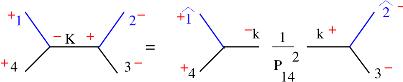
Figure 1: Factorization of the 4-point function

which is represented by the left hand side of Fig.1. With the choices already made in terms of reference momenta

$$(1234)=(+--+) = \epsilon_{3}^{-}\epsilon_{4}^{+}p_{K}^{2}\frac{1}{\frac{1}{2}P_{14}^{2}}\frac{1}{[12]\langle 12\rangle}$$ (5.17)

$$= \frac{\langle 23\rangle}{[13]}\frac{[14]}{\langle 24\rangle}[13]\langle 32\rangle[14]\langle 42\rangle\frac{1}{[14]\langle 41\rangle}\frac{1}{[12]\langle 12\rangle}$$ (5.18)

$$= \frac{\langle 23\rangle^{2}[14]}{\langle 41\rangle\langle 12\rangle[12]}\,.$$ (5.19)

Using that $[12]\langle 23\rangle=-[14]\langle 43\rangle$, which follows from momentum conservation one recovers the simple MHV expression of the 4-point function

$$(1234)=(+--+)=\frac{\langle 23\rangle^{3}}{\langle 12\rangle\langle 34\rangle\langle 41\rangle}\,.$$ (5.20)

On the other hand, we may choose to split the 4-point function into lower on-shell amplitudes, 3-point functions, as indicated on the right hand side of Fig.1. The internal leg $K$ has been put on-shell by a shift of the two external reference gluons as in (5.14), where

$$z = -\frac{P_{14}^{2}}{2\eta\cdot P_{14}}=-\frac{\langle 14\rangle[14]}{\langle 24\rangle[14]}=-\frac{\langle 14\rangle}{\langle 24\rangle}\,.$$ (5.21)

Notice that because there is no difference between the 3-point function and 3-point vertex, other than the multiplication by external line polarizations, and because we have essentially a scalar field theory, one can insert freely factors $\epsilon_{k}^{+}\epsilon_{k}^{-}$ (=1). Recalling that as argued before, the shift (5.14) in the external momenta does not modify the vertices, we see that the factorization into 3-point functions according to Fig.1. is trivially realized. Furthermore, if we follow the same steps we made earlier in converting the 3-point functions into MHV vertices, we arrive at the BCFW result.

The 5-point function is the first non-trivial example in which we invoke an identity rooted in the largest time equation. To begin with, it is given by the sum of three Feynman diagrams which are represented on the left hand side of Fig.2. The right hand side contains terms corresponding to having cut the 5-point function in all possible ways such that the reference gluons 1,5 are on opposite sides of the cut. Moreover, we shift the reference external gluons such that the cut line is on-shell. Thus the cut diagrams become on-shell amplitudes. Moreover, the cut diagrams are multiplied by the propagator of the line that was cut.

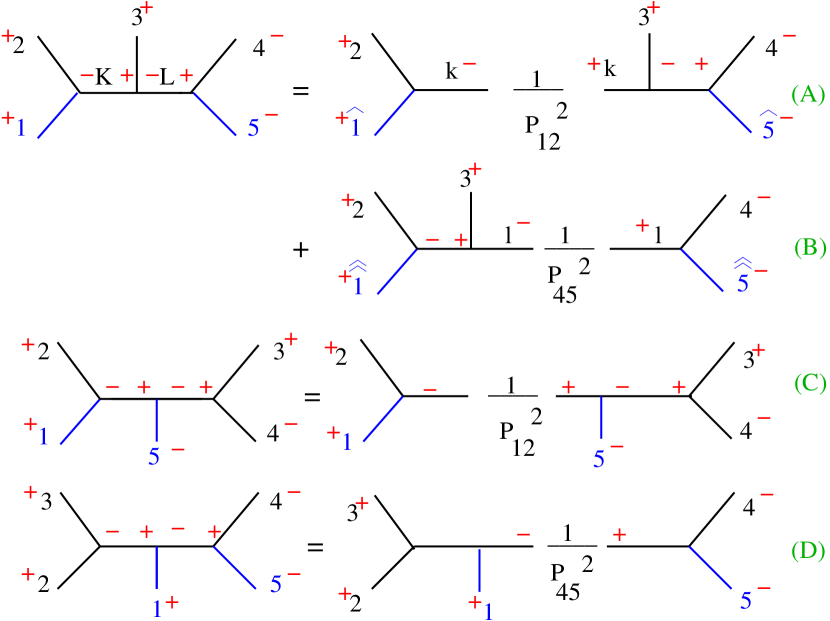
Figure 2: Factorization of the 5-point function

We will establish an identity relating the 5-point function, as computed from Feynman diagrams, to the tree amplitudes of 3 and 4-point functions as indicated by Fig.2. This, of course, is nothing but the statement of the BCFW recursion relation, applied to this particular 5-point function.

In particular we will show that the top Feynman diagram is the sum of two such cut diagrams (A+B), and that the middle and bottom Feynman diagrams are equal, respectively, with C and D. The equality of the two sides of the last two diagrams is obvious from the fact that, as argued before, the vertices on the left and right hand side of Fig.2 are the same, irrespective of having shifted the external reference momenta in order to put the cut line on shell. Moreover, the propagators on the right and left hand side of the bottom two diagrams coincide as well.

The attentive reader could observe that B+D add up to zero. After giving an obvious common factor, B+D add up to the $(+++-)$ 4-point function. The reason why we have to consider two Feynman diagrams to recover the 4-point function, as opposed to our previous calculation, is that we have selected only one of the four external gluon momenta as reference vector. This means that we have to consider both the $s$ and $t$ channel. Nonetheless, the sum of these two channels is zero, as it corresponds to having all but one external gluons of the same helicity. Thus indeed, the BCFW recursion relation amounts to including only the terms A and C, corresponding to a factorization of the $(+++--)$ amplitude into $(++-)(++--)$ amplitudes.

In the derivation of the recursion relation directly from Feynman diagrams, it is useful to keep all possible terms that arise from cutting an internal line of all Feynman diagrams, such that the reference external gluons are on opposite sides of the cut. To show that the top Feynman diagram equals A+B, once we factored out the vertices (which are the same on the left and right side of Fig.2), amounts to proving the following identity between propagators:

$$\frac{1}{P_{12}^{2}}\frac{1}{P_{45}^{2}}=\frac{1}{P_{12}^{2}}\frac{1}{P_{4\hat{5}}^{2}}+\frac{1}{P_{\hat{\hat{1}}2}^{2}}\frac{1}{P_{45}^{2}}\,,$$ (5.22)

where we defined the shifted reference gluon external momenta

$$P_{\hat{1}}=P_{1}+\hat{z}\eta,\qquad P_{\hat{5}}=P_{5}-\hat{z}\eta$$

$$P_{\hat{\hat{1}}}=P_{1}+\hat{\hat{z}}\eta,\qquad P_{\hat{\hat{5}}}=P_{5}-\hat{\hat{z}}\eta\,.$$ (5.23)

$\hat{z},\hat{\hat{z}}$ are such that we put the internal lines $K,L$, respectively, on-shell

$$\hat{z}=-\frac{P_{12}^{2}}{2\eta\cdot P_{12}}=-\frac{\langle 12\rangle}{\langle 52\rangle}$$ (5.24)

$$\hat{\hat{z}}=\frac{P_{45}^{2}}{2\eta\cdot P_{45}}=\frac{\langle 45\rangle}{\langle 15\rangle}\,,$$ (5.25)

and where the null vector $\eta$ is defined, as before, with respect to the reference gluons

$$\eta=\left|+\right\rangle\left[-\right|\equiv\left|5\right\rangle\left[1\right|\,.$$ (5.26)

Despite the fact that we can prove (5.22) by going into the bispinor basis, we find it much simpler and easily allowing for generalizations to stay in momentum space. Using that

$$P_{12}^{2}=-2\hat{z}\eta\cdot P_{12},\qquad P_{45}^{2}=2\hat{\hat{z}}\eta\cdot P_{45}$$ (5.27)

$$P_{\hat{\hat{1}}2}^{2}=2(\hat{\hat{z}}-\hat{z})\eta\cdot P_{12},\qquad P_{4\hat{5}}^{2}=2(\hat{\hat{z}}-\hat{z})\eta\cdot P_{45}\,,$$ (5.28)

(5.22) becomes a trivial algebraic identity

$$\frac{1}{\hat{z}\hat{\hat{z}}}=\frac{1}{(\hat{\hat{z}}-\hat{z})\hat{z}}-\frac{1}{(\hat{\hat{z}}-\hat{z})\hat{\hat{z}}}\,.$$ (5.29)

This completes the proof of the BCFW recursion relation from Feynman diagrams for the 5-point function and highlights the pattern that we will encounter for an arbitrary n-point function.

6 The recursion relations and the largest time equation

There is yet another way to address the identity (5.22) by rewriting the propagators in position space and next recognizing the Fourier transform of the (i.e. momentum space) largest time equation (4.4). Reinstating the usual $i\epsilon$ prescription in the momentum space propagators, and multiplying (5.22) with the total momentum conservation $\delta$-function, the right-hand-side of (5.22) becomes:

$$\frac{\delta(P_{1}+\dots+P_{5})}{P_{12}^{2}}\frac{1}{P_{45}^{2}}\! = \!\int\!x_{1}dx_{2}dx_{3}\!\int\!\frac{dK}{(2\pi)^{4}}\!\int\!\frac{dL}{(2\pi)^{4}}e^{i(P_{1}+P_{2}+K)x_{1}}e^{i(P_{3}-K+L)x_{2}}e^{i(P_{4}+P_{5}-L)x_{3}}$$ (6.1)

$$\frac{1}{K^{2}-i\epsilon}\frac{1}{L^{2}-i\epsilon}$$

$$\!= \!i^{2}\int dx_{1}dx_{2}dx_{3}\Delta(x_{1}-x_{2})\Delta(x_{2}-x_{3})e^{i(P_{1}+P_{2})x_{1}+iP_{3}x_{2}+i(P_{4}+P_{5})x_{3}}.$$

The shifted propagators which appear on the left-hand-side of (5.22) can be cast into

$$\!\!\!\!\!\!\!\!\!\!\!\!\!\frac{\delta(P_{1}+\dots+P_{5})}{P_{12}^{2}}\frac{1}{P_{4\hat{5}}^{2}}\!=\!\int\!dx_{1}dx_{2}dx_{3}\!\int\!\frac{dk}{(2\pi)^{4}}\!\int\!dz\!\int\!\frac{dL}{(2\pi)^{4}}e^{i(P_{1}+P_{2}+k)x_{1}}e^{i(P_{3}-k+L+z\eta)x_{2}}e^{i(P_{4}+P_{5}-L-z\eta)x_{3}}$$

$$\;\;\;\;\;\;\;\;\;\;\;\;\;\;\;\;\;\;\;\;\;\;\;\;\;\;\;\;\;\frac{1}{L^{2}-i\epsilon}\bigg{(}\frac{\delta^{-}((k-z\eta)^{2})}{z-i\epsilon}-\frac{\delta^{+}((k-z\eta)^{2})}{z+i\epsilon}\bigg{)}$$

$$~{}~{}~{}~{}~{}~{}~{}~{}~{}~{}~{}~{}~{}~{}~{}~{}~{}~{}~{}~{}=i^{2}\int dx_{1}dx_{2}dx_{3}e^{i(P_{1}+P_{2}+)x_{1}+iP_{3}x_{2}+i(P_{4}+P_{5})x_{3}}$$

$$~{}~{}~{}~{}~{}~{}~{}~{}~{}~{}~{}~{}~{}~{}~{}~{}~{}~{}~{}~{}\bigg{(}\theta((x_{1}-x_{3})^{+})\Delta^{+}(x_{1}-x_{2})+\theta((x_{3}-x_{1})^{+})\Delta^{-}(x_{1}-x_{2})\bigg{)}\Delta(x_{2}-x_{3}),$$ (6.2)

using the same z-parametrization which we have introduced in Section 3. For concreteness we have chosen, as before, $\eta=(\eta^{-},0,\vec{0})$ with $\eta^{-}>0$. Clearly, by integrating out first $x_{1},x_{2},x_{3}$ and using the delta-function to integrate over $k,L$, followed by a $z$-integration using the remaining delta-function $\delta((P_{1}+P_{2}-z\eta)^{2})$, we recover the left-hand-side of (6.2). On the other hand, if we choose to shift the integration variable from $k$ to $k-z\eta$, and we next integrate over $z$, then we find the result given in the last line of (6.2).

Similarly, the other term on the left-hand-side of (5.22) can be written as

$$\!\!\!\!\!\!\!\!\!\!\!\!\!\frac{\delta(P_{1}+\dots+P_{5})}{P_{1\hat{\hat{2}}}^{2}}\frac{1}{P_{45}^{2}}\!=\!\int\!dx_{1}dx_{2}dx_{3}\!\int\!\frac{dK}{(2\pi)^{4}}\!\int\!\frac{dl}{(2\pi)^{4}}\!\int\!dz\;e^{i(P_{1}+P_{2}+K+z\eta)x_{1}}e^{i(P_{3}-K-z\eta+l)x_{2}}e^{i(P_{4}+P_{5}-l)x_{3}}$$

$$\;\;\;\;\;\;\;\;\;\;\;\;\;\;\;\;\;\;\;\;\;\;\;\;\;\;\;\;\;\frac{1}{K^{2}-i\epsilon}\bigg{(}\frac{\delta^{-}((l-z\eta)^{2})}{z-i\epsilon}-\frac{\delta^{+}((l-z\eta)^{2})}{z+i\epsilon}\bigg{)}$$

$$~{}~{}~{}~{}~{}~{}~{}~{}~{}~{}~{}~{}~{}~{}~{}~{}~{}~{}~{}~{}=i^{2}\int dx_{1}dx_{2}dx_{3}e^{i(P_{1}+P_{2})x_{1}+iP_{3}x_{2}+i(P_{4}+P_{5})x_{3}}$$

$$~{}~{}~{}~{}~{}~{}~{}~{}~{}~{}~{}~{}~{}~{}~{}~{}~{}~{}~{}~{}\bigg{(}\theta((x_{1}-x_{3})^{+})\Delta^{+}(x_{2}-x_{3})+\theta((x_{3}-x_{1})^{+})\Delta^{-}(x_{2}-x_{3})\bigg{)}\Delta(x_{1}-x_{2}).$$ (6.3)

Thus the identity (5.22) becomes

$$\int \!\!\!\!\!\!\!\!\!\!\!\!\!\!dx_{1}dx_{2}dx_{3}e^{i(P_{1}+P_{2})x_{1}+iP_{3}x_{2}+i(P_{4}+P_{5})x_{3}}\bigg{[}\Delta(x_{1}-x_{2})\Delta(x_{2}-x_{3})$$ (6.4)

$$- \bigg{(}\theta((x_{1}-x_{3})^{+})\Delta^{+}(x_{1}-x_{2})+\theta((x_{3}-x_{1})^{+})\Delta^{-}(x_{1}-x_{2})\bigg{)}\Delta(x_{2}-x_{3})$$

$$- \bigg{(}\theta((x_{1}-x_{3})^{+})\Delta^{+}(x_{2}-x_{3})+\theta((x_{3}-x_{1})^{+})\Delta^{-}(x_{2}-x_{3})\bigg{)}\Delta(x_{1}-x_{2})\bigg{]}=0.$$

There is one more step that is needed in order to show the relationship between (5.22) and the largest time equation. From (4.4), with $x_{1},x_{3}$ the two vertices that are singled out, we have

$$\Delta(x_{1}-x_{2})\Delta(x_{2}-x_{3}) = \Delta^{-}(x_{1}-x_{2})\Delta^{+}(x_{2}-x_{3})$$

$$+ \theta((x_{1}-x_{3})^{+})\bigg{(}\Delta^{+}(x_{1}-x_{2})\Delta(x_{2}-x_{3})-\Delta^{*}(x_{1}-x_{2})\Delta^{+}(x_{2}-x_{3})\bigg{)}$$

$$+ \theta((x_{3}-x_{1})^{+})\bigg{(}\Delta(x_{1}-x_{2})\Delta^{-}(x_{2}-x_{3})-\Delta^{-}(x_{1}-x_{2})\Delta^{*}(x_{2}-x_{3})\bigg{)}.$$

(6.5)

To show how (6.4) is related to (6.5) we first rearrange the right-hand-side of (6.5) using

$$\Delta^{*}(x-y)=\theta((x-y)^{+})\Delta^{-}(x-y)+\theta((y-x)^{+})\Delta^{+}(x-y)\,,$$ (6.6)

such that it becomes equal to the Fourier transform of the right-hand-side of equation (6.4), up to the following two extra terms: $\theta((x_{1}-x_{3})^{+})\Delta^{+}(x_{1}-x_{2})\Delta^{+}(x_{2}-x_{3})$ and $\theta((x_{3}-x_{1})^{+})\Delta^{-}(x_{1}-x_{2})\Delta^{-}(x_{2}-x_{3})$. These terms in fact are zero as the product of the three distributions has zero support. The easiest to see this is to evaluate the Fourier transform

$$\int dx_{1}dx_{2}dx_{3}e^{i(P_{1}+P_{2})x_{1}+iP_{3}x_{2}+i(P_{4}+P_{5})x_{3}}\theta((x_{1}-x_{3})^{+})\Delta^{+}(x_{1}-x_{2})\Delta^{+}(x_{2}-x_{3})$$ (6.7)

by rewriting the step function as a $z$-integral, followed by the integration over $x_{1},x_{2},x_{3}$, to arrive at

$$\delta(P_{1}+\dots P_{5})\int dz\frac{1}{z-i\epsilon}\delta^{+}((P_{1}+P_{2}+z\eta)^{2})\delta^{+}((P_{4}+P_{5}-z\eta)^{2})\,.$$ (6.8)

It is clear that no $z$ can satisfy the simultaneously the two delta-function constraints. This completes the proof that the algebraic identity which was found by reassembling the Feynman diagrams into the BCFW recursion relations arises from the more fundamental largest time equation.

Before closing this section, we need to add some remarks to explain some more what we have accomplished. The discussion above of the largest time equation is taken for real $\eta$, since it is only for such values that we know how to order a sequence of space-time points in $\eta\cdot x_{i}$.

Now that we have the largest time equation, let us Fourier- transform it into momentum space, appropriate for a physical process under consideration and keeping $\eta$ as a variable. Then we obtain a set of shifted momenta, as in (5.23). We then analytically complexify $\eta$. For tree level, this is certainly possible and justifiable, because the dependence on it is only in some algebraic functions of propagators. At the loop level, we need to invoke the analysis of axiomatic field theorists [8], which states that there are tubes of analyticity to allow this extension and to lead to complexified unitarity relations. We now identify these propagators with the ones which we need in the space-cone gauge to carry on with the analysis.

7 The general case

To exploit the full generality of the problem, we derive an identity satisfied by the momentum space scalar propagators working under the assumption that we deal with massive propagators, with arbitrary masses.

Consider a graph at the tree level with $n^{\prime}$ vertices and $m^{\prime}$ external lines which are on-shell. As our convention, we take them to be all outgoing. We single out two of these lines which do not land on the same vertex as reference vectors and call them $p_{a}$ and $p_{b}$. For a tree graph, there is a unique path through some of the internal lines which connects $p_{a}$ to $p_{b}$. We shall denote the vertex at which $p_{a}$ emanates $x_{1}$, and that for $p_{b}$ $x_{n}$ in their space-time labels. The vertices in between are $x_{i},\ i=2,\dots n-1.$ There are then $n$ vertices in this segment of the graph and therefore n-1 internal lines. Our consideration for the time being will be on this segment. The internal lines carry momenta $q_{i}$, joining $x_{i}$ to $x_{i+1},n-1\geq i\geq 1.$ How and what other lines enter or leave these vertices need not concern us at this point. For each $q_{i}$, we associate a propagator

$$\Delta(x_{i}-x_{i+1},m_{i}) = \int{d^{4}q_{i}\over(2\pi)^{4}i}{e^{iq_{i}\cdot(x_{i}-x_{i+1})}\over q_{i}^{2}+m_{i}^{2}-i\epsilon}$$

$$= \theta(\eta\cdot(x_{i}-x_{i+1}))\Delta^{+}(x_{i}-x_{i+1},m_{i})+\theta(-\eta\cdot(x_{i}-x_{i+1}))\Delta^{-}(x_{i}-x_{i+1},m_{i})\,,$$

where

$$\Delta^{+}(x_{i}-x_{i+1},m_{i})=\int{d^{4}\bar{q}_{i}\over(2\pi)^{4}i}e^{i\bar{q}_{i}\cdot(x_{i}-x_{i+1})}\delta^{+}(\bar{q}_{i}^{2}+m_{i}^{2}),$$

$$\Delta^{-}(x_{i}-x_{i+1},m_{i})=\int{d^{4}\bar{q}_{i}\over(2\pi)^{4}i}e^{i\bar{q}_{i}\cdot(x_{i}-x_{i+1})}\delta^{-}(\bar{q}_{i}^{2}+m_{i}^{2})\,,$$ (7.2)

and where $\eta$ is a light-like vector. Due to momentum conservation, each $q_{i}$ is expressible in terms of external momenta, and in particular it has a component $+p_{a}$, or equivalently $-p_{b}$.

The factorization procedure is to cut these $q_{i}$ successively by shifting them by $z\eta$. The on-shell conditions

$$\bar{q}_{i}^{2}+m_{i}^{2}=0,\ \ \bar{q}_{i}\equiv q_{i}-z$$ (7.3)

will give us a set of solutions, points in the complex plane, namely

$$z_{i}={q_{i}^{2}+m_{i}^{2}\over 2\eta\cdot q_{i}},$$ (7.4)

for each $n-1\geq i\geq 1.$ More precisely stated, the factorization amounts to splicing the graph into a sum of products of two on-shell graphs with shifted momenta $\{p_{a}-z_{i}\eta,\dots,\bar{q}_{i}\}$ and $\{-\bar{q}_{i},\cdots,p_{b}+z_{i}\eta\}$, where $\cdots$ stand for the other momenta in the left graph segment and similarly for those in the right graph segment, with the propagator ${1\over q_{i}^{2}+m_{i}^{2}}$ as the partition. The reason that $p_{a}$ and $p_{b}$ are shifted is because we need to conserve the overall momenta on the left and the right segment separately to make them into physical amplitudes. We must demand on-shell conditions for the shifted $p_{a,b}$ with the same masses, which give

$$(p_{a}-z_{i}\eta)^{2}+m_{a}^{2}=0,\ \ \ \ \ (p_{b}+z_{i}\eta)^{2}+m_{b}^{2}=0,$$

or

$$p_{a}\cdot\eta=0,\ \ \ \ p_{b}\cdot\eta=0.$$

As $\eta$ is light-like, these conditions clearly do not allow $p_{a,b}$ to be time-like. Therefore, the two reference vectors must also be light-like, $m_{a}=m_{b}=0.$

The identity which we want to establish is

$${1\over q_{1}^{2}+m_{1}^{2}}{1\over q_{2}^{2}+m_{2}^{2}}\cdots{1\over q_{n-1}^{2}+m_{n-1}^{2}}\!\! = \!\!{1\over q_{1}^{2}+m_{1}^{2}}{1\over(q_{2}-z_{1}\eta)^{2}+m_{2}^{2}}\cdots{1\over(q_{n-1}-z_{1}\eta)^{2}+m_{n-1}^{2}}$$

$$+ \!\!{1\over(q_{1}-z_{2}\eta)^{2}+m_{1}^{2}}{1\over q_{2}^{2}+m_{2}^{2}}\cdots{1\over(q_{n-1}-z_{2}\eta)^{2}+m_{n-1}^{2}}$$

$$+ \!\!\cdots\cdots\cdots$$

$$+ \!\!\!\!{1\over(q_{1}-z_{n-1}\eta)^{2}+m_{1}^{2}}\cdots{1\over(q_{n-2}-z_{n-1}\eta)^{2}+m_{n-2}^{2}}{1\over q_{n-1}^{2}+m_{n-1}^{2}}.$$

The proof of this identity is quite simple. For $n-1\geq i\neq j\geq 1$, we write

$$(q_{i}-z_{j}\eta)^{2}+m_{i}^{2}=q_{i}^{2}+m_{i}^{2}-2z_{j}\eta\cdot q_{i}\,.$$ (7.6)

Then, using the on-shell conditions for the shifted internal momenta, which is tantamount to making cuts, we have

$$\bar{q}_{i}^{2}+m_{i}^{2}=0\ \to\ q_{i}^{2}+m_{i}^{2}=2z_{i}\eta\cdot q_{i}\,.$$ (7.7)

Together, they yield

$$(q_{i}-z_{j}\eta)^{2}+m_{i}^{2}=2\eta\cdot q_{i}(z_{i}-z_{j})\,.$$ (7.8)

Putting these together, we see the identity holds if one can show

$${(-1)^{n}\over z_{1}z_{2}\cdots z_{n-1}} = {1\over z_{1}(z_{1}-z_{2})(z_{1}-z_{3})\cdots(z_{1}-z_{n-1})}$$ (7.9)

$$+ {1\over(z_{2}-z_{1})z_{2}(z_{2}-z_{3})\cdots(z_{2}-z_{n-1})}$$

$$\cdots\cdots\cdots$$

$$+ {1\over(z_{n-1}-z_{1})(z_{n-1}-z_{2})\cdots(z_{n-1}-z_{n-2})z_{n-1}}\,.$$

This is so, because (7.9) is just a formula of partial fractioning, or it is just a statement that the integral

$$\int{dz\over z(z-z_{1})(z-z_{2})\cdots(z-z_{n-1})}=0$$

for a complex variable z over a contour which encloses all the poles.

Notice that eqn. (7) is precisely the identity needed to reassemble a generic tree level gluon Feynman diagram into lower on-shell amplitudes, as shown in Section 5. The reason for this is that, as we argued before, the vertices which enter the Feynman diagram and the corresponding lower n-point functions are the same, being insensitive to the shift of the reference gluons. Also the external line factors that have to be inserted on the cut lines to recover the lower on-shell amplitudes cancel pairwise, i.e. $\epsilon^{+}\epsilon^{-}=1$. Then, one is left to prove only an identity involving the momentum space scalar propagators. This is the same as (7), with all propagators being massless $m_{i}=0$. The combinatorics work out properly to reproduce the BCFW recursions. We have also checked these points explicitly for the six gluon amplitudes.

Furthermore, the arguments presented in Section 6, relating the momentum space identity (7) to the Fourier transform of the corresponding largest time equation (4.4), with the singled out vertices corresponding to those of the external reference gluons, can be easily carried through.

This completes our purely field theoretical proof of the BCFW recursion relations. In the process, we have identified the underlying principle behind them in the form of the largest time equation.

8 Adding massive scalars and fermions

Establishing recursion relations to include charged massive scalars is straightforward in our framework. The current interaction term $(\Phi^{*}\partial_{\mu}\Phi-\Phi\partial_{\mu}\Phi^{*})A^{\mu}$ has only $\partial^{+},\partial^{-}$ and $\partial$ derivatives, without the dangerous $\bar{\partial}$ which would have been sensitive to the shift of the external momenta, because of the space-cone gauge ($a=0$). The quartic interaction $\Phi\Phi^{*}A_{\mu}A^{\mu}$ has no momentum dependence. Therefore the vertices are unchanged under the $z\eta$ shifts. Besides there is no external line factor for scalars. This implies that we have met all the requirements to accommodate recursion relations as stressed over and again.

A more interesting and natural generalization is the inclusion of fermions in the tree level recursion relations. Consider the Lagrangian of minimally coupled massive fermions

$${\cal L}_{f}=\sum_{i}\bar{\Psi}_{i}(i/\!\!\!\nabla-m_{i})\Psi_{i}\,,$$ (8.1)

where $\nabla_{\mu}$ is the gauge covariant derivative and the Dirac matrices obey the usual anticommutation relations $\{\gamma^{\mu},\gamma^{\nu}\}=-2g^{\mu\nu}$. Then the recursion relations which are formulated with the two reference gluons connected by a path which includes a fermionic line are based on the following identity involving momentum space fermion propagators

$${1\over/\!\!\!q_{1}+m_{1}}\gamma^{\mu_{1}}{1\over/\!\!\!q_{2}+m_{2}}\gamma^{\mu_{2}}\cdots\gamma^{\mu_{n-2}}{1\over/\!\!\!q_{n-1}+m_{n-1}}$$ (8.2)

$$= {m_{1}-/\!\!\!q_{1}+z_{1}/\!\!\!\eta\over(q_{1}^{2}+m_{1}^{2})}\gamma^{\mu_{1}}{1\over/\!\!\!q_{2}-z_{1}/\!\!\!\eta+m_{2}}\gamma^{\mu_{2}}\cdots\gamma^{\mu_{n-2}}{1\over/\!\!\!q_{n-1}-z_{1}/\!\!\!\eta+m_{n-1}}$$

$$+ {1\over/\!\!\!q_{1}-z_{2}/\!\!\!\eta+m_{1}}\gamma^{\mu_{1}}{m_{2}-/\!\!\!q_{2}+z_{2}/\!\!\!\eta\over(q_{2}^{2}+m_{2}^{2})}\gamma^{\mu_{2}}\cdots\gamma^{\mu_{n-2}}{1\over/\!\!\!q_{n-1}-z_{2}/\!\!\!\eta+m_{n-1}}$$

$$+ \cdots\cdots\cdots$$

$$+ {1\over/\!\!\!q_{1}-z_{n-1}/\!\!\!\eta+m_{1}}\gamma^{\mu_{1}}\cdots\gamma^{\mu_{n-3}}{1\over/\!\!\!q_{n-2}-z_{n-1}/\!\!\!\eta+m_{n-2}}\gamma^{\mu_{n-2}}{m_{n-1}-/\!\!\!q_{n-1}+z_{n-1}/\!\!\!\eta\over(q_{n-1}^{2}+m_{n-1}^{2})}.$$

A Dirac matrix inserted between two fermion propagators corresponds to a cubic interaction vertex with a gluon field. For the case when this gluon field is an external one, one must insert external line factors and thus contract the space-time index of the Dirac matrix with that of the corresponding polarization vector. If the gluon field corresponds to an internal line, then we must contract the space-time index of the Dirac matrix with that of the gluon propagator. At this stage it is important to stress that we are in the space-cone gauge, such that $\eta\cdot A=0$, which means that $/\!\!\!\eta/\!\!\!A=-/\!\!\!A/\!\!\!\eta$. Thus in (7) we consider only insertions of Dirac matrices which effectively anticommute with the null vector $\eta$.

The proof of (8.2) relies partly on one identity which we have already established, namely (7). First rewrite the fermionic propagators such that all denominators will correspond to scalar propagators. Next cancel out in the numerator all terms with at least one insertion of $/\!\!\!\eta$. This can be done, since $/\!\!\!\eta/\!\!\!\eta=0$, corroborated with the previous observation that $/\!\!\!\eta$ and $\gamma^{\mu}$ anticommute. Finally, we need to employ one other algebraic identity, namely

$$\int dz\frac{z^{m}}{(z-z_{1})(z-z_{2})\dots(z-z_{n-1})}=0,\;{\rm for}\;m<n-2\,,$$ (8.3)

where the integral is evaluated over a contour which encircles all the poles. As mentioned many times before, the structure of the vertices is unchanged by the shift with $z_{i}\eta$ in the momenta of the reference gluons. We complete the proof of the recursion relations by observing that each term in (8.2) corresponds to a factorization into lower on-shell amplitudes, such that each propagator belonging on the path that connects the two reference external gluons is cut and put on-shell, accompanied by the corresponding shift of the external gluons. The left and right amplitudes are multiplied by the propagator of the line which was cut. The reason why in the recursion relations the “cut” fermionic lines have an extra factor $m_{i}-/\!\!\!q_{i}+z_{i}/\!\!\!\eta$ has to do with the fact that this corresponds exactly to the appropriate insertion of the external line factors.

Thus we have provided a field theoretical proof of the recursion relations for massive scalars and fermions found by [9, 10].

9 Conclusions

To summarize our results, we have shown that the BCFW recursion relations can be proven starting from the standard gauge theory Feynman diagrams. Perhaps the only less familiar ingredient is the use of a certain convenient gauge, space-cone. We have shown that each tree level gluon Feynman diagram “factorizes”, i.e. it can be written as a sum of product of lower on-shell amplitudes that arise from successive cuts of all internal lines which connect two reference gluons. To be able to still satisfy the momentum conservation laws, the momenta of the reference gluons must be shifted in a particular way. Moreover, the amplitudes arising from cuts must be multiplied by the propagator of the line which was cut. The proof of factorization is based, among other things, on an algebraic identity involving the momentum space propagators, which we recognized as the complexified Fourier transform of the largest time equation.

Let us recall that the largest time equations are exact identities in quantum field theories, independent of loop levels. They yielded results for spectral representation of two-point functions, side-wise dispersion relations for vertex functions, etc. We may infer from these examples that exploiting them in the area of complexified unitarity to complement space-cone gauge freedom should likely offer new opportunities at the loop level for organizing QCD computations, among other things. In particular, it should facilitate a field theoretical perspective of the one-loop recursion relations [11].

We have also addressed generalizations of the tree level BCFW recursion relations involving massive charged scalars and fermions, proving them in a purely field theoretical setup.

Note added

While this manuscript was being written, we became aware of [12] which has partial overlap with our results.

References

- [1] E. Witten, Commun. Math. Phys. 252, 189 (2004) [arXiv:hep-th/0312171].
- [2] F. Cachazo, P. Svrcek and E. Witten, JHEP 0409, 006 (2004) [arXiv:hep-th/0403047].
- [3] R. Britto, F. Cachazo and B. Feng, Nucl. Phys. B 715, 499 (2005) [arXiv:hep-th/0412308].
- [4] R. Britto, F. Cachazo, B. Feng and E. Witten, Phys. Rev. Lett. 94, 181602 (2005) [arXiv:hep-th/0501052].
- [5] Z. Bern, L. J. Dixon, D. C. Dunbar and D. A. Kosower, Nucl. Phys. B 435, 59 (1995) [arXiv:hep-ph/9409265].
- [6] G. Chalmers and W. Siegel, Phys. Rev. D 59, 045013 (1999) [arXiv:hep-ph/9801220].
- [7] M. J. G. Veltman, Physica 29, 186 (1963).
- [8] R. F. Streater and A. S. Wightman, PCT, Spin & Statics and all that, The Mathematical Physics Monograph Series, ed. W. A. Benjamin, Inc (1964).
- [9] S. D. Badger, E. W. N. Glover, V. V. Khoze and P. Svrcek, JHEP 0507, 025 (2005) [arXiv:hep-th/0504159].
- [10] S. D. Badger, E. W. N. Glover and V. V. Khoze, arXiv:hep-th/0507161.
- [11] Z. Bern, L. J. Dixon and D. A. Kosower, Phys. Rev. D 71, 105013 (2005) [arXiv:hep-th/0501240].
- [12] P. D. Draggiotis, R. H. P. Kleiss, A. Lazopoulos and C. G. Papadopoulos, arXiv:hep-ph/0511288.