Hawking Radiation of the Brane-Localized Graviton from a $(4+n)$-dimensional Black Hole

Abstract

Following the Regge-Wheeler algorithm, we derive a radial equation for the brane-localized graviton absorbed/emitted by the $(4+n)$-dimensional Schwarzschild black hole. Making use of this equation the absorption and emission spectra of the brane-localized graviton are computed numerically. Existence of the extra dimensions generally suppresses the absorption rate and enhances the emission rate as other spin cases. The appearance of the potential well, however, when $n>\sqrt{\ell(\ell+1)-2}-1$ in the effective potential makes the decreasing behavior of the total absorption with increasing $n$ in the low-energy regime. The high-energy limit of the total absorption cross section seems to coincide with that of the brane-localized scalar cross section. The increasing rate of the graviton emission is very large compared to those of other brane-localized fields. This fact indicates that the graviton emission can be dominant one in the Hawking radiation of the higher-dimensional black holes when $n$ is large.

The most striking result of the modern brane-world scenarios[1] is the emergence of the TeV-scale gravity when the extra dimensions exist. This fact opens the possibility to make the tiny black holes in the future high-energy colliders[2] on condition that the large or warped extra dimensions exist. In this reason the absorption and emission problems for the higher-dimensional black holes were extensively explored recently.

The absorption and emission spectra for the brane-localized spin $0$, $1/2$ and $1$ particles and the bulk scalar in the $(4+n)$-dimensional Schwarzschild phase were numerically examined in Ref[3]. The main motivation of Ref.[3] is to check the issue[4] whether or not the black holes radiate mainly on the brane. The result of the numerical calculation strongly supports the argument made by Emparan, Horowitz and Myers(EHM), i.e. the emission on the brane is dominant compared to that off the brane.

In Ref.[5] different numerical method was applied to examine the absorption and emission spectra of the brane-localized and bulk scalars in the background of the higher-dimensional charged black hole. The numerical method used in Ref.[5] is an application of the quantum mechanical scattering method incorporated with an analytic continuation, which was used in Ref.[6] to compute the spectra of the massless and massive scalars in the $4d$ Schwarzschild background. The numerical result of Ref.[5] also supports the argument made by EHM if the number of the extra dimensions is not too large.

However, it was argued in Ref.[7] that the argument of EHM should be examined carefully in the rotating black hole background because there is an another important factor called superradiance[8] if the black holes have the angular momenta. Especially, in Ref.[7] the existence of the superradiant modes was explicitly proven in the scattering of the bulk scalar when the spacetime background is a $5$-dimensional rotating black hole with two angular momentum parameters. The general criteria for the existence of the superradiant modes were derived in Ref.[9] when the bulk scalar, electromagnetic and gravitational waves are absorbed by the higher-dimensional rotating black hole with arbitrarily multiple angular momentum parameters.

The Hawking radiation on the brane is also examined when the bulk black hole has an angular momentum[10]. Numerical calculation supports the fact that the superradiance modes also exist in the brane emission. Thus the brane emission and bulk emission were compared with each other in Ref.[11] when the scalar field interacts with a $5$-dimensional rotating black hole. It was shown that although the superradiance modes exist in the bulk emission in the wide range of energy, the energy amplification for the bulk scalar is extremely small compared to the energy amplification for the brane scalar. As a result the effect of the superradiance modes is negligible and does not change the EHM’s claim.

There is an another factor we should take into account carefully in the Hawking radiation of the higher-dimensional black holes. This is an higher spin effect like a graviton emission. Since the graviton is not generally localized on the brane unlike the standard model particles, the argument of the EHM should be carefully checked in the graviton emission. Recently, the bulk graviton emission was explored in Ref.[12] when the background is an higher-dimensional Schwarzschild black hole. In this paper we would like to examine the absorption and emission problems for the brane-localized graviton in the background of the $(4+n)$-dimensional Schwarzschild black hole.

We start with a metric induced by a $(4+n)$-dimensional Schwarzschild spacetime[13]

$$ds_{\mbox{ind}}^{2}=-h(r)dt^{2}+h^{-1}(r)dr^{2}+r^{2}(d\theta^{2}+\sin^{2}\theta d\phi^{2})$$ (1)

where $h(r)=1-(r_{H}/r)^{n+1}$. Of course, $r_{H}$ is a parameter which denotes the radius of the event horizon and the Hawking temperature is given by $T_{H}=(n+1)/4\pi r_{H}$. To derive an equation which governs the gravitational fluctuation we should change the metric itself. Following the Regge-Wheeler algorithm[14] we introduce the gravitational fluctuation by adding the metric component

$$\delta s^{2}=\left[H_{0}(r)dtd\phi+H_{1}(r)drd\phi\right]e^{i\omega t}\sin\theta\frac{dP_{\ell}}{d\theta}(\cos\theta)$$ (2)

to the original metric $ds_{\mbox{ind}}^{2}$. Of course, we should assume $H_{0},H_{1}<<1$ for the linearizarion.

Now, we would like to discuss how to derive the fluctuation equation. Since the metric (1) is an usual Schwarzschild metric when $n=0$, it is a vacuum solution of the Einstein equation. For the $4d$ case, therefore, the fluctuation equation can be expressed as $\delta R_{\mu\nu}=0$, where $R_{\mu\nu}$ is a Ricci tensor. For $n\neq 0$ case, however, the metric (1) is not a vaccum solution. Thus, we should assume that the metric (1) is a non-vacuum solution of the $4d$ Einstein equation, i.e. ${\cal E}_{\mu\nu}=T_{\mu\nu}$ where ${\cal E}_{\mu\nu}$ and $T_{\mu\nu}$ are Einstein tensor and the non-vanishing energy-momentum tensor. Adding the metric perturbation (2) to the original metric (1) the Einstein equation would be changed into $\delta{\cal E}_{\mu\nu}=\delta T_{\mu\nu}$. The main problem in the derivation of the fluctuation equation is the fact that we do not know the nature of the matter because the non-vanishing energy-momentum tensor is not originated from the real matter on the brane but appears effectively in the course of the projection of the bulk metric to the brane. Thus the difficulty is how to derive $\delta T_{\mu\nu}$ without knowing the real nature of the matter.

Firstly, we should note that the linear order perturbation yields only non-vanishing $\delta{\cal E}_{t\phi}$, $\delta{\cal E}_{r,\phi}$ and $\delta{\cal E}_{\theta\phi}$ in the gravity side. Thus it is reasonable to assume that the non-vanishing components of $\delta T_{\mu\nu}$ are $\delta T_{t\phi}$, $\delta T_{r\phi}$ and $\delta T_{\theta\phi}$. The corresponding components of the Einstein equation are

$$-\frac{1}{4}h(r)\frac{d^{2}H_{0}}{dr^{2}}+\left(\frac{\lambda+h}{2r^{2}}+\frac{1}{2r}\frac{dh}{dr}+\frac{1}{4}\frac{d^{2}h}{dr^{2}}\right)H_{0}+\frac{i\omega}{4}h(r)\left(\frac{dH_{1}}{dr}+\frac{2}{r}H_{1}\right)=\delta\Theta_{t\phi}$$ (3)

$$-\frac{i\omega}{4}h^{-1}(r)\left(\frac{dH_{0}}{dr}-\frac{2}{r}H_{0}\right)+\left[\frac{\lambda}{2r^{2}}-\frac{\omega^{2}}{4}h^{-1}(r)+\frac{1}{2r}\frac{dh}{dr}+\frac{1}{4}\frac{d^{2}h}{dr^{2}}\right]H_{1}=\delta\Theta_{r\phi}$$ (4)

$$\hskip 85.35826pti\omega h^{-1}(r)H_{0}-h(r)\frac{dH_{1}}{dr}-\frac{dh}{dr}H_{1}=4\delta\Theta_{\theta\phi}$$ (5)

where $\lambda=(\ell+2)(\ell-1)/2$ and

$$\delta T_{t\phi}=\delta\Theta_{t\phi}(r)e^{i\omega t}\sin\theta\frac{dP_{\ell}}{d\theta}(\cos\theta)$$ (6)

$$\delta T_{r\phi}=\delta\Theta_{r\phi}(r)e^{i\omega t}\sin\theta\frac{dP_{\ell}}{d\theta}(\cos\theta)$$ (7)

$$\delta T_{\theta\phi}=\delta\Theta_{\theta\phi}(r)e^{i\omega t}\left(\cos\theta\frac{d}{d\theta}-\sin\theta\frac{d^{2}}{d\theta^{2}}\right)P_{\ell}(\cos\theta).$$ (8)

The conservation of the energy-momentum tensor yields a constraint

$$\frac{i\omega}{r^{2}}h^{-1}(r)\delta\Theta_{t\phi}-\frac{1}{r^{2}}h(r)\left[\partial_{r}\delta\Theta_{r\phi}+\left(h^{-1}(r)\frac{dh}{dr}+\frac{2}{r}\right)\delta\Theta_{r\phi}\right]-\frac{2\lambda}{r^{4}}\delta\Theta_{\theta\phi}$$ (11)

$$=\frac{i\omega}{2r^{3}}h^{-1}(r)\left(\frac{dh}{dr}+\frac{r}{2}\frac{d^{2}h}{dr^{2}}\right)H_{0}-\frac{1}{2r^{3}}h(r)\left(\frac{dh}{dr}+\frac{r}{2}\frac{d^{2}h}{dr^{2}}\right)\frac{dH_{1}}{dr}$$

$$\hskip 14.22636pt-\frac{1}{r^{3}}\left[\frac{1}{2}\frac{dh}{dr}\left(\frac{dh}{dr}+\frac{r}{2}\frac{d^{2}h}{dr^{2}}\right)+h(r)\left(\frac{1}{2r}\frac{dh}{dr}+\frac{d^{2}h}{dr^{2}}+\frac{r}{4}\frac{d^{3}h}{dr^{3}}\right)\right]H_{1}.$$

It is easy to show that as expected the rhs of Eq.(11) is zero when $n=0$. Another constraint may be derived from the fact that only two of three equations in Eq.(3) should be linearly independent. However, it does not yield a new constraint because it is possible to derive the first equation of (3) from the remaining ones if (11) is used. Final requirement is that the effective potential derived from Eq.(3) should coincide with the usual Regge-Wheeler potential when $n=0$. This restriction gives a constraint

$$\lim_{n\rightarrow 0}\delta\Theta_{t\phi}=\lim_{n\rightarrow 0}\delta\Theta_{r\phi}=\lim_{n\rightarrow 0}\delta\Theta_{\theta\phi}=0.$$ (12)

As far as we know, we cannot make any more constraint for the energy-momentum tensor from the general principle. Of course the constraints (11) and (12) are not sufficient to fix $\delta\Theta_{t\phi}$, $\delta\Theta_{r\phi}$ and $\delta\Theta_{\theta\phi}$ completely. Thus we cannot determine the effective potential due to the lack of knowledge on the matter content. Thus what we can do is to choose $\delta\Theta_{\mu\nu}$ consistently with Eq.(11) and (12).

We will choose $\delta\Theta_{r\phi}=\delta\Theta_{\theta\phi}=0$ with a hope that the detailed shape of the effective potential does not change the graviton emissivity drastically. Eliminating $H_{0}$ in Eq.(3), one can derive a differential equation for solely $H_{1}$ in the form

$$\frac{d^{2}H_{1}}{dr^{2}}+\left(3h^{-1}(r)\frac{dh}{dr}-\frac{2}{r}\right)\frac{dH_{1}}{dr}$$ (13)

$$\hskip 28.45274pt+\left[\left(\omega^{2}+\left(\frac{dh}{dr}\right)^{2}\right)h^{-2}(r)-\left(\frac{\ell(\ell+1)-2}{r^{2}}+\frac{4}{r}\frac{dh}{dr}\right)h^{-1}(r)\right]H_{1}=0.$$ (14)

Now, it is convenient to introduce a function $R(r)$ defined as $H_{1}\equiv r^{2}h^{-1}(r)R$. Then the fluctuation equation (13) reduces to

$$\frac{h(r)}{r^{2}}\frac{d}{dr}\left(r^{2}h(r)\frac{dR}{dr}\right)+\left[\omega^{2}-h(r)\left\{\frac{\ell(\ell+1)}{r^{2}}-\epsilon\left(\frac{2}{r^{2}}(1-h(r))-\frac{d^{2}h}{dr^{2}}\right)\right\}\right]R.$$ (15)

In Eq.(15) we introduced a parameter $\epsilon$. When $\epsilon=1$, Eq.(15) corresponds to the gravitational fluctuation and $\epsilon=0$ corresponds to the scalar fluctuation. Thus one can treat the scalar and gravitational fluctuations in an unified way. We used $\epsilon$ to confirm our numerical calculation which will be carried out later. Putting $\epsilon=0$, we checked our numerical calculation reproduces the absorption and emission spectra of the brane-localized scalar calculated in Ref.[3, 5].

Defining again $R=\Psi/r$, Eq.(15) is transformed into the Schrödinger-like equation

$$\left(h(r)\frac{d}{dr}\right)^{2}\Psi+\left[\omega^{2}-V_{\mbox{eff}}(r)\right]\Psi=0$$ (16)

where the effective potential is

$$V_{\mbox{eff}}(r)=h(r)\left[\frac{\ell(\ell+1)}{r^{2}}+\frac{1}{r}\frac{dh}{dr}-\epsilon\left(\frac{2}{r^{2}}\left(1-h(r)\right)-\frac{d^{2}h}{dr^{2}}\right)\right].$$ (17)

It is worthwhile noting that until this stage we have not used the explicit expression of $h(r)$. Thus we can use the equations derived above for the gravitational fluctuation of any $4d$-induced spherically symmetric metric. Using an explicit expression of $h(r)$, one can easily show

$$V_{\mbox{eff}}(r)=h(r)\left[\frac{\ell(\ell+1)}{r^{2}}-\frac{\sigma_{n}r_{H}^{n+1}}{r^{n+3}}\right]$$ (18)

where $\sigma_{n}=\epsilon[(n+1)(n+2)+2]-(n+1)$. When $n=0$, the effective potential (18) reduces to the usual Regge-Wheeler potential. Defining a “tortoise” coordinate $z$ as $dz/dr=h^{-1}(r)$, the wave equation (16) simply reduces to

$$\frac{d^{2}\Psi}{dz^{2}}+\left[\omega^{2}-V_{\mbox{eff}}(r)\right]\Psi=0.$$ (19)

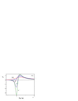
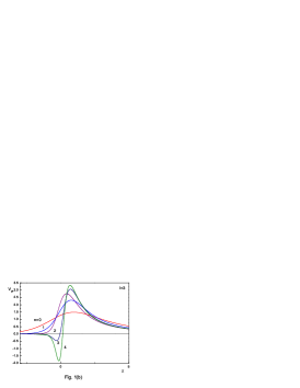
FIG. 1.: The $z$-dependence of the effective potential for the brane-localized graviton. Fig. 1(a) and (b) correspond to $\ell=2$(the lowest mode) and $\ell=3$ respectively. For fixed $\ell$ each potential with $n<\ell$ has a barrier whose height increases with increasing $n$. When $n\geq\ell$, each potential has a barrier in the side of the asymptotic region and a well in the opposite side. The emergence of this potential well in the effective potential seems to affect the low-energy behavior of the cross sections.

The effective potential for the gravitational fluctuation, i.e. $\epsilon=1$,is plotted as a function of $z$ in Fig. 1 when $\ell=2$ (Fig. 1(a)) and $\ell=3$ (Fig. 1(b)). For the lowest mode $\ell=2$ each potential with $n<\ell$ has a barrier whose height increases with increasing $n$. Thus the existence of the extra dimensions should suppress the absorption rate. Each potential with $n\geq\ell$ has a barrier in the side of the asymptotic region and a well in the opposite side. When $n$ increases, the barrier and well become higher and deeper respectively. While, therefore, the barrier tends to decrease the absorption rate with increasing $n$, the well tends to enhance it. Thus, the absorption cross section should be determined by the competition between the barrier and the well. The effective potential with $\ell=3$ exhibits a similar behavior as Fig. 2(b) shows.

The absorption cross section for $\ell=2$ and $3$ is plotted in Fig. 2 when $n=0$, $1$, and $2$. Fig. 2 indicates that overall, the existence of the extra dimensions suppresses the absorption rate as other fields. This means that the potential barrier is more important factor than the potential well in determining the absorption rate. However, Fig. 2(a) shows that the cross section for $n=2$ is larger than that for $n=0$ or $1$ in the low-$\omega$ region. This means that the potential well plays more important role in this region.

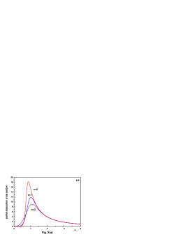
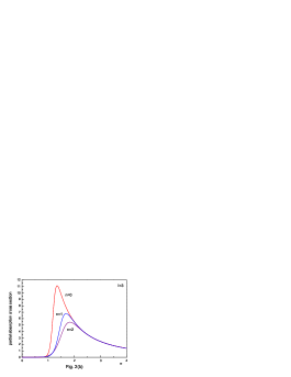
FIG. 2.: The $\omega$-dependence of the partial absorption cross sections for $\ell=2$(Fig. 2(a)) and $\ell=3$(Fig. 2(b)). Overall, the existence of the extra dimensions suppresses the absorption rate as in the cases of other fields. However, the reversion of the magnitude in the low-energy regime of Fig. 2(a) seems to be due to the emergence of the potential well in the effective potential.

Now we would like to explain how to compute the physical quantities related to the absorption and emission of the brane-localized graviton. Since the numerical method used in this paper was extensively used in Ref.[5, 6, 11], we will just comment it schematically. Using the dimensionless parameters $x\equiv\omega r$ and $x_{H}\equiv\omega r_{H}$, the radial equation (15) can be written as

$$\hskip 56.9055ptx^{2}(x^{n+1}-x_{H}^{n+1})^{2}\frac{d^{2}R}{dx^{2}}+x(x^{n+1}-x_{H}^{n+1})\left[2x^{n+1}+(n-1)x_{H}^{n+1}\right]\frac{dR}{dx}$$ (20)

$$+\left[x^{2n+4}-\ell(\ell+1)x^{n+1}(x^{n+1}-x_{H}^{n+1})+\epsilon\left\{(n+1)(n+2)+2\right\}x_{H}^{n+1}(x^{n+1}-x_{H}^{n+1})\right]R=0.$$ (21)

Due to the real nature of Eq.(20), $R^{\ast}$ should be a solution if $R$ is a solution of Eq.(20). The Wronskian between them is

$$W[R^{\ast},R]_{x}\equiv R^{\ast}\frac{dR}{dx}-R\frac{dR^{\ast}}{dx}=\frac{{\cal{C}}x^{n-1}}{x^{n+1}-x_{H}^{n+1}}$$ (22)

where ${\cal{C}}$ is an integration constant. Since $x=x_{H}$ is a regular singular point of the differential equation (20), we can solve Eq.(20) to obtain a solution which is convergent in the near-horizon regime as following:

$${\cal{G}}_{n,\ell}(x,x_{H})=e^{\lambda_{n}\ln|x-x_{H}|}\sum_{N=0}^{\infty}d_{\ell,N}(x-x_{H})^{N}$$ (23)

where $\lambda_{n}=-ix_{H}/(n+1)$. Of course, the recursion relation can be directly derived by inserting Eq.(23) into the radial equation (20). The Wronskian between ${\cal{G}}^{\ast}$ and ${\cal{G}}$ is same with Eq.(22) with ${\cal{C}}=-2i|d_{\ell,0}|^{2}x_{H}^{2}$. In Ref.[6] the relation between $|d_{\ell,0}|^{2}$ and the partial transmission coefficient ${\cal{T}}_{n,\ell}$

$$|d_{\ell,0}|^{2}=\frac{(\ell+1/2)^{2}}{x_{H}^{2}}{\cal{T}}_{n,\ell}$$ (24)

is derived by making use of the quantum mechanical scattering theory.

The ingoing and outgoing solutions which are convergent in the asymptotic regime can be derived directly also as series expressions in the form

$${\cal{F}}_{n,\ell(\pm)}(x,x_{H})=(\pm i)^{\ell+1}e^{\mp ix}(x-x_{H})^{\pm\lambda_{n}}\sum_{N=0}^{\infty}\tau_{N(\pm)}x^{-(N+1)}.$$ (25)

The Wronskian between ${\cal{F}}_{(+)}$ and ${\cal{F}}_{(-)}$ is same with Eq.(22) with ${\cal{C}}=2i$.

Since the asymptotic solution is a linear combination of the ingoing and outgoing solutions, one can assume that the scattering solution which is convergent at the asymptotic region is

$${\cal{R}}_{n,\ell}(x,x_{H})=f_{n,\ell}^{(-)}(x_{H}){\cal{F}}_{n,\ell(+)}(x,x_{H})+f_{n,\ell}^{(+)}(x_{H}){\cal{F}}_{n,\ell(-)}(x,x_{H})$$ (26)

where the coefficients $f_{n,\ell}^{(\pm)}$ are called the jost functions. It should be noted that if we know ${\cal{R}}$, the jost functions can be computed by the Wronskian as following:

$$f_{n,\ell}^{(\pm)}(x_{H})=\pm\frac{x^{n+1}-x_{H}^{n+1}}{2ix^{n-1}}W[{\cal{F}}_{n,\ell(\pm)},{\cal{R}}_{n,\ell}]_{x}.$$ (27)

In Ref.[6] the relation between the jost functions and the coefficient $d_{\ell,0}$ is also derived in the form

$$d_{\ell,0}=\frac{\ell+1/2}{f_{n,\ell}^{(-)}}.$$ (28)

Combining Eq.(24) and (28) the partial absorption cross section can be written as

$$\sigma_{\ell}^{BR}\equiv\frac{\pi}{\omega^{2}}(2\ell+1){\cal{T}}_{\ell}=\frac{\pi(2\ell+1)r_{H}^{2}}{|f_{n,\ell}^{(-)}(x_{H})|^{2}}$$ (29)

where the superscript denotes the brane-localized graviton.

The emission spectrum, i.e. the energy emitted per unit time, is given by the Hawking formula

$$\Gamma^{BR}=\frac{\omega^{3}\sigma_{abs}^{BR}}{2\pi^{2}(e^{\omega/T_{H}}-1)}d\omega$$ (30)

where $\sigma_{abs}^{BR}$ is a total absorption cross section. Thus the absorption and emission spectra can be completely computed if we know the jost functions. In Ref.[5, 6, 11] the function ${\cal{R}}$ is computed numerically from the near-horizon solution (23) by increasing the convergence region via the analytic continuation. Then Eq.(27) enables us to compute the jost functions numerically. This is an overall algorithm of our numerical technique.

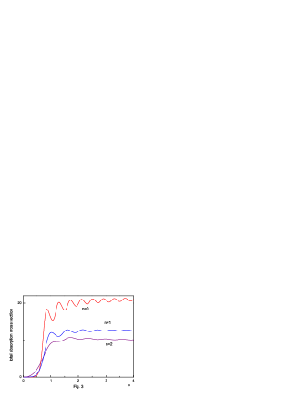
FIG. 3.: The $\omega$-dependence of the total absorption cross sections for the brane-localized graviton. Overall, the existence of the extra dimensions suppresses the total absorption cross sections. The low-energy behavior of this figure also implies the crucial effect of the potential well emerged when $n\geq\ell$.

The total absorption cross section is plotted in Fig. 3 when $n=0$, $1$ and $2$. As in the case of the scalar field absorption the existence of the extra dimensions in general suppresses the absorption rate. This indicates that the potential barrier is more important factor in determining the absorption cross section. However, the low-$\omega$ region of Fig. 3 seems to indicate that the emergence of the potential well when $n\geq\ell$ crucially changes the order of magnitude. The wiggly pattern indicates that each partial absorption cross section has a peak point at different $\omega$. The high-energy limits of the total cross sections seem to coincide with the scalar case, i.e.

$$\lim_{\omega\rightarrow\infty}\sigma_{abs}^{BR}=\left(\frac{n+3}{2}\right)^{2/(n+1)}\frac{n+3}{n+1}\pi r_{H}^{2}.$$ (31)

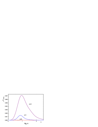
FIG. 4.: The $\omega$-dependence of the emission rate when $n=0$, $1$, and $2$. As in the cases of other fields the existence of the extra dimensions generally enhances the emissivities. The emission spectrum for $n=0$ cannot be seen clearly because it is too small compared to other cases. The drastic change of the emission rate indicates that the graviton emission can be a dominant one in the Hawking radiation of the higher-dimensional black holes for large $n$.

The emission spectrum of the graviton is plotted in Fig. 4. As in the case of the scalar emission the existence of the extra dimensions enhances the emission rate. This indicates that the Planck factor is most important in determining the emission rate. For $n=0$ the emission spectrum cannot be seen clearly in Fig. 4 because it is too small compared to the other cases. The drastic increase of the emission rate implies that the Hawking radiation of the higher spin becomes more and more important for large $n$.

	$n=0$	$n=1$	$n=2$
graviton	$7.67\times 10^{-6}$	$8.06\times 10^{-4}$	$6.70\times 10^{-3}$
scalar	$2.98\times 10^{-4}$	$2.66\times 10^{-3}$	$1.07\times 10^{-2}$
graviton/scalar	$0.026$	$0.303$	$0.624$

Table I

The total emission rate $\int\Gamma^{BR}$ for graviton and scalar is summarized in Table I. Generally the total emission rate for the graviton is smaller than that for the scalar. But the ratio between them tends to increase dramatically with increasing $n$. Thus we can conjecture that for large $n$ the graviton radiation becomes dominant in the Hawking radiation of the higher-dimensional black holes.

In this paper we studied the absorption and emission of the brane-localized graviton in the context of the brane-world scenarios. The existence of the extra dimensions in general tends to suppress the total absorption cross section as the cases of other fields. In the low-energy region, however, the order of the magnitude is reversed (see Fig. 3). This seems to be due to the emergence of the well in the effective potential. The high-energy limits of the total cross sections for the brane-localized gravitons seem to coincide with those for the brane-localized massless scalars.

As in the cases of other fields the existence of the extra dimensions generally enhances the emission rate. This fact indicates that the Planck factor is most dominant term in determining the emissivities. However, the increasing rate of the brane-localized graviton is very large compared to those of other fields. To show this explicitly, the increasing rates of the brane-localized graviton and scalar is given in Table I. This rapid increase of the emissivity indicates that the graviton emission should be dominant radiation in the Hawking radiation of the higher-dimensional black holes when $n$ is large.

It is straightforward to extend our calculation to the higher-dimensional charged black hole background by choosing

$$h(r)=\left[1-\left(\frac{r_{+}}{r}\right)^{n+1}\right]\left[1-\left(\frac{r_{-}}{r}\right)^{n+1}\right]$$ (32)

where $r_{\pm}$ correspond to the outer and inner horizons. Since we have not used the explicit expression of $h(r)$ when deriving Eq.(15), we can use the radial equation (15) with only choosing different $h(r)$. The introduction of the inner horizon parameter $r_{-}$ changes the Hawking temperature into

$$T_{H}=\frac{n+1}{4\pi r_{+}^{n+2}}\left(r_{+}^{n+1}-r_{-}^{n+1}\right).$$ (33)

When, therefore, $r_{-}$ increases, the Hawking temperature becomes lower, which should enhance the absorptivity and reduce the emission rate. Since the introduction of the extra dimensions generally suppresses the absorptivity and enhances the emission rate, the exact absorption and emission spectra for the charged black hole case may be determined by the competition between $r_{-}$ and $n$.

Recently, in Ref.[12] the absorption rate for the bulk graviton is studied in the Schwarzschild background. The fluctuations for the bulk graviton have three different modes, i.e. scalar, vector, and tensor modes. It is of greatly interest to apply our method to compare the emission rate for the brane-localized graviton with that for the bulk graviton.

Acknowledgement: This work was supported by the Kyungnam University Research Fund, 2006.

REFERENCES

- [1] N. Arkani-Hamed, S. Dimopoulos and G. Dvali, The Hierarchy Problem and New Dimensions at a Millimeter, Phys. Lett. B429 (1998) 263 [hep-ph/9803315]; L. Antoniadis, N. Arkani-Hamed, S. Dimopoulos and G. Dvali, New Dimensions at a Millimeter to a Fermi and Superstrings at a TeV, Phys. Lett. B436 (1998) 257 [hep-ph/9804398]; L. Randall and R. Sundrum, A Large Mass Hierarchy from a Small Extra Dimension, Phys. Rev. Lett. 83 (1999) 3370 [hep-ph/9905221]; L. Randall and R. Sundrum, An Alternative to Compactification, Phys. Rev. Lett. 83 (1999) 4690 [hep-th/9906064].
- [2] S. B. Giddings and T. Thomas, High energy colliders as black hole factories: The end of short distance physics, Phys. Rev. D65 (2002) 056010 [hep-ph/0106219]; S. Dimopoulos and G. Landsberg, Black Holes at the Large Hadron Collider, Phys. Rev. Lett. 87 (2001) 161602 [hep-ph/0106295]; D. M. Eardley and S. B. Giddings, Classical black hole production in high-energy collisions, Phys. Rev. D66 (2002) 044011 [gr-qc/0201034]; D. Stojkovic, Distinguishing between the small ADD and RS black holes in accelerators, Phys. Rev. Lett. 94 (2005) 011603 [hep-ph/0409124]; V. Cardoso, E. Berti and M. Cavaglià, What we (don’t) know about black hole formation in high-energy collisions, Class. Quant. Grav. 22 (2005) L61 [hep-ph/0505125].
- [3] C. M. Harris and P. Kanti, Hawking Radiation from a -dimensional Black Hole: Exact Results for the Schwarzschild Phase, JHEP 0310 (2003) 014 [hep-ph/0309054]; P. kanti, Black Holes in Theories with Large Extra Dimensions: a Review, Int. J. Mod. Phys. A19 (2004) 4899 [hep-ph/0402168].
- [4] P. Argyres, S. Dimopoulos and J. March-Russell, Black Holes and Sub-millimeter Dimensions, Phys. Lett. B441 (1998) 96 [hep-th/9808138]; T. Banks and W. Fischler, A Model for High Energy Scattering in Quantum Gravity [hep-th/9906038]; R. Emparan, G. T. Horowitz and R. C. Myers, Black Holes radiate mainly on the Brane, Phys. Rev. Lett. 85 (2000) 499 [hep-th/0003118].
- [5] E. Jung and D. K. Park, Absorption and Emission Spectra of an higher-dimensional Reissner-Nordström black hole, Nucl. Phys. B717 (2005) 272 [hep-th/0502002].
- [6] N. Sanchez, Absorption and emission spectra of a Schwarzschild black hole, Phys. Rev. D18 (1978) 1030; E. Jung and D. K. Park, Effect of Scalar Mass in the Absorption and Emission Spectra of Schwarzschild Black Hole, Class. Quant. Grav. 21 (2004) 3717 [hep-th/0403251].
- [7] V. Frolov and D. Stojković, Black hole radiation in the brane world and the recoil effect, Phys. Rev. D66 (2002) 084002 [hep-th/0206046]; V. Frolov and D. Stojković, Black Hole as a Point Radiator and Recoil Effect on the Brane World, Phys. Rev. Lett. 89 (2002) 151302 [hep-th/0208102]; V. Frolov and D. Stojković, Quantum radiation from a -dimensional black hole, Phys. Rev. D67 (2003) 084004 [gr-qc/0211055].
- [8] Y. B. Zel’dovich, Generation of waves by a rotating body, JETP Lett. 14 (1971) 180; W. H. Press and S. A. Teukolsky, Floating Orbits, Superradiant Scattering and the Black-hole Bomb, Nature 238 (1972) 211; A. A. Starobinskii, Amplification of waves during reflection from a rotating black hole, Sov. Phys. JETP 37 (1973) 28; A. A. Starobinskii and S. M. Churilov, Amplification of electromagnetic and gravitational waves scattered by a rotating black hole, Sov. Phys. JETP 38 (1974) 1.
- [9] E. Jung, S. H. Kim and D. K. Park, Condition for Superradiance in Higher-dimensional Rotating Black Holes, Phys. Lett. B615 (2005) 273 [hep-th/0503163]; E. Jung, S. H. Kim and D. K. Park, Condition for the Superradiance Modes in Higher-Dimensional Black Holes with Multiple Angular Momentum Parameters, Phys. Lett. B619 (2005) 347 [hep-th/0504139].
- [10] D. Ida, K. Oda and S. C. Park, Rotating black holes at future collider: Greybody factors for brane field, Phys. Rev. D67 (2003) 064025 [hep-th/0212108]; C. M. Harris and P. Kanti, Hawking Radiation from a -Dimensional Rotating Black Hole [hep-th/0503010]; D. Ida, K. Oda and S. C. Park, Rotating black holes at future colliders II : Anisotropic scalar field emission, Phys. Rev. D71 (2005) 124039 [hep-th/0503052]; G. Duffy, C. Harris, P. Kanti and E. Winstanley, Brane decay of a -dimensional rotating black hole: spin- particle, JHEP 0509 (2005) 049 [hep-th/0507274]; M. Casals, P. Kanti and E. Winstanley, Brane Decay of a -Dimensional Rotating Black Hole II: spin- particles [hep-th/0511163].
- [11] E. Jung and D. K. Park, Bulk versus Brane in the Absorption and Emission: D Rotating Black Hole Case, Nucl. Phys. B731 (2005) 171 [hep-th/0506204].
- [12] A. S. Cornell, W. Naylor and M. Sasaki, Graviton emission from a higher-dimensional black hole [hep-th/0510009].
- [13] F. R. Tangherlini, Schwarzschild Field in Dimensions and the Dimensionality of Space Problem, Nuovo Cimento 27 (1963) 636; R. C. Myers and M. J. Perry, Black Holes in Higher Dimensional Space-Times, Ann. Phys. 172 (1986) 304.
- [14] T. Regge and J. A. Wheeler, Stability of a Schwarzschild Singularity, Phys. Rev. 108 (1957) 1063; C. V. Vishveshwara, Stability of the Schwarzschild Metric, Phys. Rev. D 1 (1970) 2870; L. A. Edelstein and C. V. Vishveshwara, Differential Equations for Perturbations on the Schwarzschild Metric, Phys. Rev. D 1 (1970) 3514; C. V. Vishveshwara, Scattering of Gravitational Radiation by a Schwarzschild Black-hole, Nature 227 (1970) 936.
- [15] F. J. Zerilli, Effective Potential for even-parity Regge-Wheeler Gravitational Perturbation Equations, Phys. Rev. Lett. 24 (1970) 737.