On Transgression Forms and Chern–Simons (Super)gravity

Abstract

A transgression form is proposed as lagrangian for a gauge field theory. The construction is first carried out for an arbitrary Lie Algebra $\mathfrak{g}$ and then specialized to some particular cases. We exhibit the action, discuss its symmetries, write down the equations of motion and the boundary conditions that follow from it, and finally compute conserved charges. We also present a method, based on the iterative use of the Extended Cartan Homotopy Formula, which allows one to (i) systematically split the lagrangian in order to appropriately reflect the subspaces structure of the gauge algebra, and (ii) separate the lagrangian in bulk and boundary contributions. Chern–Simons Gravity and Supergravity are then used as examples to illustrate the method. In the end we discuss some further theoretical implications that arise naturally from the mathematical structure being considered.

I Introduction

The motivations for the study of higher-dimensional Gravity  have remained largely invariant since B. Zumino’s paper Gravity Theories in more than four dimensions Zum85 ; we may add here that String Theory (ST) has since grown into an all-encompassing framework that guides and inspires research in high-energy physics. Among its rich offspring, ST provides with a gravity lagrangian which includes, at higher-order corrections in $\alpha^{\prime}$, higher powers of the curvature tensor. The potential incompatibilities between the ghost particles usually associated with these terms and the ghost-free ST were first analyzed in Zwi85 , where it was pointed out that a proper combination of curvature-squared terms leads to ‘ghost-free, non-trivial gravitational interactions for dimensions higher than four’. The key point, already conjectured by Zwiebach, and confirmed later by Zumino, is that the allowed terms in $d$ dimensions are the dimensional continuations of all the Euler densities of dimension lower than $d$. For even $d$, one has the seemingly odd choice of also adding the Euler density corresponding to $d$, which, being a total derivative, does not contribute to the equations of motion. However, this term is crucial in order to attain a proper regularization for the conserved charges (like mass and angular momentum) Zan99 ; Zan00 . Interestingly enough, the ghost-free, higher-power-in-curvature lagrangians considered by Zumino had been introduced much earlier, in a completely classical context, by D. Lovelock Lov70 (it is also noteworthy the contribution of C. Lanczos, Ref. Lan38 ).

Lanczos–Lovelock (LL) lagrangians have been extensively studied (for some recent work, check, e.g., Des05 ; Zeg05 ; Hen05 ; Wil04 ; Aie05 ; Iza04 ; All03 ; Sal03 ; Aro00 ; Cri00 ). There are typically  $1+\left[d/2\right]$ ghost-free LL lagrangians in $d$ dimensions, which can be linearly combined, with arbitrary coefficients $\alpha_{p}$, $p=0,1,\ldots,\left[d/2\right]$, into a full-fledged gravity lagrangian. The first term in the series, without any curvature contributions $\left(p=0\right)$, corresponds to a cosmological term, while the second one, linear in curvature $\left(p=1\right)$, is nothing else than the usual Einstein–Hilbert (EH) lagrangian.

The next major step in our programme is the embedding of the full LL lagrangian into the broader scheme of Chern–Simons (CS) theory. As first shown by Chamseddine Cha89 ; Cha90 and Bañados, Teitelboim and Zanelli Ban93 , there is a special choice of the $\alpha_{p}$ coefficients that brings the LL lagrangian in odd dimensions only a total derivative away from a CS lagrangian. To be more explicit, take $\bm{A}$ to be a $\mathfrak{so}\left(d+1\right)$-valued, one-form gauge connection  and pick the Levi-Civita symbol $\varepsilon$ as an invariant tensor. The CS lagrangian built with these two ingredients is then equal to a LL lagrangian (with the chosen coefficients) plus a total derivative.

An alternative way of deriving these ‘canonical’ coefficients rests on the physical requirement of well-defined dynamics Tro99 . This argument can also be made in even dimensions, where the resulting lagrangian has a Born–Infeld-like form, leading to the associated theory being dubbed ‘Born–Infeld (BI) Gravity’. Conserved charges for even-dimensional BI gravity can be computed via a direct application of Noether’s Theorem Zan99 ; Zan00 . The formula so obtained correctly reproduces mass and angular momentum for a host of exact solutions, without requiring regularization or the subtraction of an ad-hoc background. This success is however harder to replicate for their odd-dimensional counterpart, CS gravity. Naïve application of Noether’s Theorem yields in this case a formula for the charges that fails to give the physically correct values for at least one solution. A beautiful resolution of this uncomfortable situation has been recently proposed by Mora, Olea, Troncoso and Zanelli in Mor04 ; Ole04 . They add a carefully selected boundary term to the CS action which renders it both finite and capable of producing well-defined charges. Although this boundary term is deduced from purely gravitational arguments, the last paragraph in Mor04 already points to the ultimate reason for the action’s remarkable properties: it can be regarded as a transgression form.

Transgression forms are the matrix where CS forms stem from Nak03 ; Azc95 . In this paper we shall be mainly concerned with the formulation of what may be called Transgression Gauge Field Theory (TGFT); i.e., a classical, gauge field theory whose lagrangian is a transgression form.

The organization of the paper goes as follows. In section II we briefly review CS Theory and comment on its relation to the Chern–Weil theorem. Section III brings in the transgression form as a lagrangian for a gauge field theory. We discuss its symmetries, write down the equations of motion and the boundary conditions that follow from it, and finally compute conserved charges. LL Gravity is recovered as a first example in section IV. The Extended Cartan Homotopy Formula (ECHF) is presented in section V, and in section VI it is shown to be an extremely useful tool in formulating gravity and supergravity. Finally, important theoretical issues are given some thought in section VII.

II Chern–Simons Theory: A Review

Let $\mathfrak{g}$ be a Lie algebra over some field. Essential objects in everything that follows will be $\mathfrak{g}$-valued differential forms on some space-time manifold $M$, which we shall denote by italic boldface. When $\bm{P}$ is a $p$-form and $\bm{Q}$ is a $q$-form, then its Lie bracket $\left[\cdot,\cdot\right]$ has the following symmetry:

$$\left[\bm{P},\bm{Q}\right]=\left(-1\right)^{pq}\left[\bm{Q},\bm{P}\right].$$ (1)

Given the Lie bracket and a one-form $\bm{A}$ it is always possible to define a ‘covariant derivative’ D as

$$\text{D}\bm{Z}\equiv\text{d}\bm{Z}+\left[\bm{A},\bm{Z}\right],$$ (2)

where d denotes the usual exterior derivative. This covariant derivative has the (defining) property that, if $\bm{Z}$ transforms as a tensor and $\bm{A}$ as a connection under $\mathfrak{g}$, then D$\bm{Z}$ will also transform as a tensor.

Let $\left\langle\cdots\right\rangle_{r}$ denote a $\mathfrak{g}$-invariant symmetric polynomial

$$\left\langle\cdots\right\rangle_{r}:\;\underset{r}{\underbrace{\mathfrak{g\times\cdots\times g}}}\;\rightarrow\mathbb{C}$$ (3)

of some fixed rank $r$. The invariance requirement for $\left\langle\cdots\right\rangle_{r}$ essentially boils down to 

$$\left\langle\text{D}\left(\bm{Z}_{1}\cdots\bm{Z}_{r}\right)\right\rangle_{r}=\text{d}\left\langle\bm{Z}_{1}\cdots\bm{Z}_{r}\right\rangle_{r},$$ (4)

where $\left\{\bm{Z}_{k},k=1,\ldots,r\right\}$ is a set of $\mathfrak{g}$-valued differential forms. The symmetry requirement for $\left\langle\cdots\right\rangle_{r}$ implies that, for any $p$-form $\bm{P}$ and $q$-form $\bm{Q}$, we have

$$\left\langle\cdots\bm{PQ}\cdots\right\rangle_{r}=\left(-1\right)^{pq}\left\langle\cdots\bm{QP}\cdots\right\rangle_{r}.$$ (5)

This remains valid even in the case of $\mathfrak{g}$ being a superalgebra, due to the Grassmann nature of the parameters that multiply fermionic generators.

In what follows we shall usually drop the subscript $r$ in the invariant polynomial, as we will only use one fixed rank (to be specified below).

A CS lagrangian in $d=2n+1$ dimensions is defined to be the following local function  of a one-form gauge connection $\bm{A}$:

$$L_{\text{CS}}^{\left(2n+1\right)}\left(\bm{A}\right)=\left(n+1\right)k\int_{0}^{1}dt\left\langle\bm{A}\left(t\text{d}\bm{A}+t^{2}\bm{A}^{2}\right)^{n}\right\rangle,$$ (6)

where $\left\langle\cdots\right\rangle$ denotes a $\mathfrak{g}$-invariant symmetric polynomial of rank $r=n+1$ and $k$ is a constant. One important fact to note here is that CS forms are only locally defined. To see this, we have to consider the following result Nak03 ; Azc95 :

Theorem 1

(Chern–Weil). Let $\bm{A}$ and $\bar{\bm{A}}$ be two one-form gauge connections on a fiber bundle over a $\left(2n+1\right)$-dimensional manifold $M$, and let $\bm{F}$ and $\bar{\bm{F}}$ be the corresponding curvatures. Then, with the above notation,

$$\left\langle\bm{F}^{n+1}\right\rangle-\left\langle\bar{\bm{F}}^{n+1}\right\rangle=\text{d}Q_{\bm{A}\leftarrow\bar{\bm{A}}}^{\left(2n+1\right)},$$ (7)

where

$$Q_{\bm{A}\leftarrow\bar{\bm{A}}}^{\left(2n+1\right)}\equiv\left(n+1\right)\int_{0}^{1}dt\left\langle\bm{\theta F}_{t}^{n}\right\rangle$$ (8)

is called a transgression form and we have defined

$$\bm{\theta} \equiv\bm{A}-\bar{\bm{A}},$$ (9)

$$\bm{A}_{t} \equiv\bar{\bm{A}}+t\bm{\theta},$$ (10)

$$\bm{F}_{t} \equiv\text{d}\bm{A}_{t}+\bm{A}_{t}^{2}.$$ (11)

A sketch of the proof is given in Appendix A in order to get an intuitive, ‘physical’ sense of the theorem’s content. The theorem is also deduced as a corollary of the ECHF in section V.1.

Setting $\bar{\bm{A}}=0$ in (8) gives the CS form as

$$Q^{\left(2n+1\right)}\left(\bm{A}\right) =Q_{\bm{A}\leftarrow 0}^{\left(2n+1\right)},$$

$$=\left(n+1\right)\int_{0}^{1}dt\left\langle\bm{A}\left(t\text{d}\bm{A}+t^{2}\bm{A}^{2}\right)^{n}\right\rangle.$$ (12)

The Chern–Weil theorem for this particular case shows that d$\delta Q^{\left(2n+1\right)}\left(\bm{A}\right)=0$; this implies that $\delta Q^{\left(2n+1\right)}\left(\bm{A}\right)$ may be locally written as d$\Omega$ for some $\Omega$ under gauge transformations. But since a connection cannot be globally set to zero unless the bundle (topology) is trivial, CS forms turn out to be only locally defined. Of course, this is only a problem if one insists on using a CS form as a lagrangian, since then one has to integrate it over all of $M$ to get the action. Nevertheless, CS forms are used as lagrangians mainly because (i) they lead to gauge theories with a fiber-bundle structure, whose only dynamical field is a one-form gauge connection $\bm{A}$ and (ii) they do change by only a total derivative under gauge transformations. When we choose $\mathfrak{g}=\mathfrak{so}\left(2n+2\right)$ and write $\bm{A}$ as

$$\bm{A}=e^{a}\bm{P}_{a}+\frac{1}{2}\omega^{ab}\bm{J}_{ab},$$ (13)

then the CS form provides with a background-free gravity theory (since metricity is given by the vielbein, which is just one component of $\bm{A}$). An explicit realization of $d=11$ Supergravity (SUGRA) in terms of a CS lagrangian has even shed some new light on the old problem of why our world seems to be four-dimensional Has03 ; Has05 .

On the other hand, a transgression form is in principle globally well defined and also, as we will see, invariant under gauge transformations. We now turn to the discussion of transgression forms used as lagrangians for gauge field theories — TGFT.

III The Transgression Form as a Lagrangian

III.1 TGFT Field Equations

We consider a gauge theory on an orientable $\left(2n+1\right)$-dimensional manifold $M$ defined by the action

$$S_{\text{T}}^{\left(2n+1\right)}\left[\bm{A},\bar{\bm{A}}\right] =k\int_{M}Q_{\bm{A}\leftarrow\bar{\bm{A}}}^{\left(2n+1\right)}$$

$$=\left(n+1\right)k\int_{M}\int_{0}^{1}dt\left\langle\bm{\theta F}_{t}^{n}\right\rangle,$$ (14)

where $k$ is a constant (see previous section for notation and conventions). Eq. (14) describes (the dynamics of) a theory with two independent fields, namely the two one-form gauge connections $\bm{A}$ and $\bar{\bm{A}}$. These fields enter the action in a rather symmetrical way; for instance, interchange of both connections produces a sign difference, i.e.,

$$S_{\text{T}}^{\left(2n+1\right)}\left[\bar{\bm{A}},\bm{A}\right]=-S_{\text{T}}^{\left(2n+1\right)}\left[\bm{A},\bar{\bm{A}}\right].$$ (15)

A striking new feature of the action (14) is the presence of two independent one-form gauge connections, $\bm{A}$ and $\bar{\bm{A}}$. The physical interpretation of this will be made clear in the next sections through several examples, which we discuss in some detail.

Performing independent variations of $\bm{A}$ and $\bar{\bm{A}}$ in (14) we get after some algebra (see Appendix B)

$$\delta S_{\text{T}}^{\left(2n+1\right)}=\left(n+1\right)k\int_{M}\left(\left\langle\delta\bm{AF}^{n}\right\rangle-\left\langle\delta\bar{\bm{A}}\bar{\bm{F}}^{n}\right\rangle\right)+\int_{\partial M}\Theta,$$ (16)

with

$$\Theta=n\left(n+1\right)k\int_{0}^{1}dt\left\langle\delta\bm{A}_{t}\bm{\theta F}_{t}^{n-1}\right\rangle.$$ (17)

This result (but for the exact form of the boundary term $\Theta$) may be readily guessed just by looking at the Chern–Weil theorem. An explicit computation gives us (17).

The TGFT field equations can be directly read off from the variation (16). They are

$$\left\langle\bm{F}^{n}\bm{G}_{a}\right\rangle =0,$$ (18)

$$\left\langle\bar{\bm{F}}^{n}\bm{G}_{a}\right\rangle =0,$$ (19)

where $\left\{\bm{G}_{a},a=1,\ldots,\dim\left(\mathfrak{g}\right)\right\}$ is a basis for $\mathfrak{g}$. Boundary conditions are obtained by demanding the vanishing of $\Theta$ on $\partial M$:

$$\left.\int_{0}^{1}dt\left\langle\delta\bm{A}_{t}\bm{\theta F}_{t}^{n-1}\right\rangle\right|_{\partial M}=0.$$ (20)

Eqs. (18)–(20) tell us about two independent CS theories living on a manifold $M$ which are inextricably linked at the boundary. Below we shall see some examples where this story is told, albeit in a rather simple and surprising way.

III.2 Symmetries

There are two major independent symmetries lurking in our TGFT action, eq. (14). The first of them is a built-in symmetry, guaranteed from the outset by our use of differential forms throughout: it is diffeomorphism invariance. Although straightforward, the symmetry is far-reaching, as is proved by the fact that it leads to non-trivial conserved charges.

The second symmetry is gauge symmetry. Under a continuous, local gauge transformation generated by a group element $g=\exp\left(\lambda^{a}\bm{G}_{a}\right)$, the connections change as

$$\bm{A} \rightarrow\bm{A}^{\prime}=g\left(\bm{A}-g^{-1}\text{d}g\right)g^{-1},$$ (21)

$$\bar{\bm{A}} \rightarrow\bar{\bm{A}}^{\prime}=g\left(\bar{\bm{A}}-g^{-1}\text{d}g\right)g^{-1}.$$ (22)

Invariance of the TGFT lagrangian under (21)–(22) is guaranteed by (i) the fact that both $\bm{\theta}$ and $\bm{F}_{t}$ transform as tensors and (ii) the invariant nature of the symmetric polynomial $\left\langle\cdots\right\rangle$.

Crucially, and in stark contrast with the CS case, there are no boundary terms left after the gauge transformation: the TGFT action (14) is fully invariant rather than pseudo-invariant. A pseudo-invariant lagrangian is one that changes by a closed form under gauge transformations. In this case the lagrangian ceases to be univocally defined; quite naturally, the addition of an arbitrary exact form cannot be ruled out on the grounds of symmetry alone. A direct consequence is an inherent ambiguity in the boundary conditions that must follow from the action. Any conserved charges computed from a pseudo-invariant lagrangian will also be changed by this modification, rendering them also ambiguous. A TGFT suffers from none of this problems; we cannot add an arbitrary closed form to the Lagrangian, since that would destroy the symmetry. This means that the charges and boundary conditions derived from the TGFT action are in principle physically meaningful.

III.3 Conserved Charges

In order to fix the notation and conventions, we briefly review here Noether’s Theorem in the language of differential forms Zan99 ; Zan00 . Let $L\left(\varphi\right)$ be a lagrangian $d$-form for some set of fields $\varphi$. An infinitesimal functional variation $\delta\varphi$ induces an infinitesimal variation $\delta L$,

$$\delta L=E\left(\varphi\right)\delta\varphi+\text{d}\Theta\left(\varphi,\delta\varphi\right),$$ (23)

where $E\left(\varphi\right)=0$ are the equations of motion and $\Theta$ is a boundary term which depends on $\varphi$ and its variation $\delta\varphi$. When $\delta\varphi$ corresponds to a gauge transformation, the off-shell variation of $L$ equals (at most) a total derivative, $\delta L=$ d$\Omega$. Noether’s Theorem then states that the current 

$$\left.\star J_{\text{gauge}}\right.=\Omega-\Theta\left(\varphi,\delta_{\text{gauge}}\varphi\right)$$ (24)

is on-shell conserved; i.e., d$\left.\star J_{\text{gauge}}\right.=0$. An analogous statement is valid for a diffeomorphism generated by a vector field $\xi$, $\delta x^{\mu}=\xi^{\mu}\left(x\right)$. In this case the conserved current has the form 

$$\left.\star J_{\text{diff}}\right.=-\Theta\left(\varphi,\delta_{\text{diff}}\varphi\right)-\text{I}_{\xi}L.$$ (25)

In eqs. (24) and (25) it is understood that we replace in $\Theta$ the variation of $\varphi$ corresponding to the gauge transformation or the diffeomorphism, respectively.

When formulæ (24)–(25) are applied to the TGFT lagrangian [cf. eq. (14)]

$$L_{\text{T}}^{\left(2n+1\right)}=\left(n+1\right)k\int_{0}^{1}dt\left\langle\bm{\theta F}_{t}^{n}\right\rangle,$$ (26)

the following conserved currents are obtained (see Appendix C for a derivation):

$$\left.\star J_{\text{gauge}}\right. =n\left(n+1\right)k\text{d}\int_{0}^{1}dt\left\langle\bm{\lambda\theta F}_{t}^{n-1}\right\rangle,$$ (27)

$$\left.\star J_{\text{diff}}\right. =n\left(n+1\right)k\text{d}\int_{0}^{1}dt\left\langle\text{I}_{\xi}\bm{A}_{t}\bm{\theta F}_{t}^{n-1}\right\rangle.$$ (28)

Here $\bm{\lambda}$ is a local, $\mathfrak{g}$-valued 0-form parameter that defines an infinitesimal gauge transformation via $\delta\bm{A}=-$D${}_{\bm{A}}\bm{\lambda}$, $\delta\bar{\bm{A}}=-$D${}_{\bar{\bm{A}}}\bm{\lambda}$ and $\xi$ is a vector field that generates an infinitesimal diffeomorphism, which acts on $\bm{A}$ and $\bar{\bm{A}}$ as $\delta\bm{A}=-\pounds_{\xi}\bm{A}$, $\delta\bar{\bm{A}}=-\pounds_{\xi}\bar{\bm{A}}$. In writing (27) and (28) we have dropped terms proportional to the equations of motion, so that the currents are only defined on-shell. This allows writing them as total derivatives, a step which renders verification of the conservation law d$\left.\star J\right.=0$ trivial.

Assuming the space-time manifold $M$ to have the topology $M=\mathbb{R}\times\Sigma$, we can integrate (27) and (28) over the ‘spatial section’ $\Sigma$ to get the conserved charges

$$Q_{\text{gauge}} =n\left(n+1\right)k\int_{\partial\Sigma}\int_{0}^{1}dt\left\langle\bm{\lambda\theta F}_{t}^{n-1}\right\rangle,$$ (29)

$$Q_{\text{diff}} =n\left(n+1\right)k\int_{\partial\Sigma}\int_{0}^{1}dt\left\langle\text{I}_{\xi}\bm{A}_{t}\bm{\theta F}_{t}^{n-1}\right\rangle.$$ (30)

Stokes’ Theorem allows us to restrict the integration to the boundary of the spatial section $\Sigma$.

To summarize, we have given explicit formulæ to compute conserved charges for the TGFT lagrangian as integrals over the boundary of an spatial section in space-time. The general proof of finiteness for these charges remains as an open problem; however, examples already exist where this is explicitly confirmed Mor04 .

The charges (29) and (30) are trivially invariant under diffeomorphisms, since they’re built out of differential forms. Invariance under gauge transformations is slightly less straightforward; under $\delta\bm{A}=-$D$\bm{\lambda}$, $Q_{\text{gauge}}$ remains invariant and $Q_{\text{diff}}$ transforms as

$$\delta_{\bm{\lambda}}Q_{\text{diff}}=-n\left(n+1\right)k\int_{\partial\Sigma}\int_{0}^{1}dt\left\langle\pounds_{\xi}\bm{\lambda\theta F}_{t}^{n-1}\right\rangle.$$ (31)

From (31) we see that a sufficient condition to ensure invariance of $Q_{\text{diff}}$ under gauge transformations is to demand the transformation to satisfy $\pounds_{\xi}\bm{\lambda}=0$ on $\partial\Sigma$. That is, $Q_{\text{diff}}$ is invariant under those restricted gauge transformations that fulfill this condition.

As a final remark on the charge formulæ (29)–(30), we would like to point out that both $Q_{\text{gauge}}$ and $Q_{\text{diff}}$ flip signs under the interchange $\bm{A}\leftrightarrows\bar{\bm{A}}$; we may then interpret this operation as ‘charge conjugation’.

IV An Example: LL Gravity as a TGFT

As already mentioned in the Introduction, the lagrangian for odd-dimensional LL gravity with the canonical coefficients is only a total derivative away from a CS form. To see this, consider for definiteness the AdS Algebra in $d=2n+1$ dimensions,

$$\left[\bm{P}_{a},\bm{P}_{b}\right] =\frac{1}{\ell^{2}}\bm{J}_{ab},$$ (32)

$$\left[\bm{J}_{ab},\bm{P}_{c}\right] =\eta_{cb}\bm{P}_{a}-\eta_{ca}\bm{P}_{b},$$ (33)

$$\left[\bm{J}_{ab},\bm{J}_{cd}\right] =\eta_{cb}\bm{J}_{ad}-\eta_{ca}\bm{J}_{bd}+\eta_{db}\bm{J}_{ca}-\eta_{da}\bm{J}_{cb},$$ (34)

where $\ell$ is a length (the AdS radius). The $\mathfrak{so}\left(2n,2\right)$-valued one-form gauge connection has the form

$$\bm{A}=e^{a}\bm{P}_{a}+\frac{1}{2}\omega^{ab}\bm{J}_{ab},$$ (35)

where we identify $e^{a}$ with the vielbein and $\omega^{ab}$ with the spin connection.

There are several choices one can make for an invariant polynomial; perhaps the simplest of them is the one for which

$$\left\langle\bm{J}_{a_{1}a_{2}}\cdots\bm{J}_{a_{2n-1}a_{2n}}\bm{P}_{a_{2n+1}}\right\rangle=\frac{2^{n}}{\ell}\varepsilon_{a_{1}\cdots a_{2n+1}},$$ (36)

with all other combinations vanishing.

When we use the connection (35) and the invariant polynomial (36) in the general formula for the CS form, eq. (6), we get the LL lagrangian with the canonical coefficients plus a total derivative. What we would like to point out here is that this LL lagrangian, without the total derivative coming from the CS form, may also be regarded as a Transgression form. As a matter of fact, when we choose

$$\bm{A} =\frac{1}{2}\omega^{ab}\bm{J}_{ab}+e^{a}\bm{P}_{a},$$ (37)

$$\bar{\bm{A}} =\frac{1}{2}\omega^{ab}\bm{J}_{ab},$$ (38)

and the same invariant tensor (36), then the TGFT lagrangian [cf. eq. (14)] reads Cha89 ; Cha90

$$L_{\bm{\omega}+\bm{e}\leftarrow\bm{\omega}}^{\left(2n+1\right)} =\left(n+1\right)\frac{k}{\ell}\varepsilon_{a_{1}\cdots a_{2n+1}}\times$$

$$\times\int_{0}^{1}dtF_{t}^{a_{1}a_{2}}\cdots F_{t}^{a_{2n-1}a_{2n}}e^{a_{2n+1}},$$ (39)

where

$$F_{t}^{ab}=R^{ab}+\frac{t^{2}}{\ell^{2}}e^{a}e^{b}.$$ (40)

From eq. (39) we learn that the choice (36) of invariant symmetric polynomial effectively amounts to excluding the torsion from appearing explicitly in the lagrangian (although it is not assumed to vanish). It is interesting to note that the $t$-integration in (39) manages to exactly reproduce the canonical coefficients for the LL polynomial Ban93 .

It is not at all obvious that the TGFT lagrangian (39) and the CS lagrangian (6) should differ only by a total derivative. The fact that they do is associated with the particular form of the invariant polynomial used in both cases, namely the Levi-Civita tensor. In fact, let us recall that the CS lagrangian locally satisfies

$$\text{d}L_{\text{CS}}^{\left(2n+1\right)}=k\left\langle\bm{F}^{n+1}\right\rangle,$$ (41)

whereas the TFGT lagrangian satisfies

$$\text{d}L_{\bm{\omega}+\bm{e}\leftarrow\bm{\omega}}^{\left(2n+1\right)}=k\left(\left\langle\bm{F}^{n+1}\right\rangle-\left\langle\bar{\bm{F}}^{n+1}\right\rangle\right).$$ (42)

Our choice for the invariant polynomial now implies that

$$\left\langle\bar{\bm{F}}^{n+1}\right\rangle=0,$$

and we see that both lagrangians can only differ the way they do. This kind of structure for the invariant polynomial $\left\langle\cdots\right\rangle$ will have important consequences, as we will see in the next sections.

V The Extended Cartan Homotopy Formula

In principle, the TGFT lagrangian in its full generality [cf. eq. (14)],

$$L_{\bm{A}\leftarrow\bar{\bm{A}}}^{\left(2n+1\right)}=\left(n+1\right)k\int_{0}^{1}dt\left\langle\bm{\theta F}_{t}^{n}\right\rangle,$$ (43)

has all the information one needs about the theory; as shown in section III, it is possible to write down general expressions for the equations of motion, the boundary conditions and the conserved charges without ever bothering to say what the gauge group is supposed to be. In practice, however, one often deals with a fixed gauge group or supergroup with several distinct subgroups which have an individual, clear physical meaning. It would then be desirable to have a systematic procedure to split the lagrangian (43) into pieces that reflect this group structure.

In this section we discuss a tool on which a separation method can be built (see section VI). Let us begin by noticing that, according to the Chern–Weil Theorem (see section II), the following combination of derivatives of transgression forms identically vanishes:

$$\text{d}Q_{\bm{A}\leftarrow\bar{\bm{A}}}^{\left(2n+1\right)}+\text{d}Q_{\tilde{\bm{A}}\leftarrow\bm{A}}^{\left(2n+1\right)}+\text{d}Q_{\bar{\bm{A}}\leftarrow\tilde{\bm{A}}}^{\left(2n+1\right)}$$

$$=\left\langle\bm{F}^{n+1}\right\rangle-\left\langle\bar{\bm{F}}^{n+1}\right\rangle+$$

$$+\left\langle\tilde{\bm{F}}^{n+1}\right\rangle-\left\langle\bm{F}^{n+1}\right\rangle+$$ (44)

$$+\left\langle\bar{\bm{F}}^{n+1}\right\rangle-\left\langle\tilde{\bm{F}}^{n+1}\right\rangle$$ (45)

$$=0.$$ (46)

Here $\bm{A}$, $\tilde{\bm{A}}$ and $\bar{\bm{A}}$ are three arbitrary, one-form gauge connections, with $\bm{F}$, $\tilde{\bm{F}}$ and $\bar{\bm{F}}$ being the corresponding curvatures. This vanishing further implies that we can (at least locally) write

$$Q_{\bm{A}\leftarrow\bar{\bm{A}}}^{\left(2n+1\right)}+Q_{\tilde{\bm{A}}\leftarrow\bm{A}}^{\left(2n+1\right)}+Q_{\bar{\bm{A}}\leftarrow\tilde{\bm{A}}}^{\left(2n+1\right)}=\text{d}Q_{\bm{A}\leftarrow\tilde{\bm{A}}\leftarrow\bar{\bm{A}}}^{\left(2n\right)},$$ (47)

where $Q_{\bm{A}\leftarrow\tilde{\bm{A}}\leftarrow\bar{\bm{A}}}^{\left(2n\right)}$ is a $2n$-form which depends on all three connections and whose explicit form cannot be directly determined from the Chern–Weil Theorem alone. Now we recast the ‘triangle’ equation (47) in a more suggestive way as

$$Q_{\bm{A}\leftarrow\bar{\bm{A}}}^{\left(2n+1\right)}=Q_{\bm{A}\leftarrow\tilde{\bm{A}}}^{\left(2n+1\right)}+Q_{\tilde{\bm{A}}\leftarrow\bar{\bm{A}}}^{\left(2n+1\right)}+\text{d}Q_{\bm{A}\leftarrow\tilde{\bm{A}}\leftarrow\bar{\bm{A}}}^{\left(2n\right)},$$ (48)

which can be read off as saying that a transgression form ‘interpolating’ between $\bar{\bm{A}}$ and $\bm{A}$ may be written as the sum of two transgressions which introduce an intermediate, ancillary one-form $\tilde{\bm{A}}$ plus a total derivative. It is important to note here that $\tilde{\bm{A}}$ is completely arbitrary, and may be chosen according to convenience. Eq. (48), used iteratively if necessary, allows us to split our TGFT lagrangian essentially at wish — note however that every use of (48) brings in a boundary contribution which is so far not known.

In order to obtain an explicit form for $Q_{\bm{A}\leftarrow\tilde{\bm{A}}\leftarrow\bar{\bm{A}}}^{\left(2n\right)}$, and also to show the common origin of the Chern–Weil Theorem and the Triangle Equation (48), we recall here a powerful result known as the Extended Cartan Homotopy Formula (ECHF) Man85 .

Let us consider a set $\left\{\bm{A}_{i},i=0,\ldots,r+1\right\}$ of one-form gauge connections on a fiber-bundle over a $d$-dimensional manifold $M$ and a $\left(r+1\right)$-dimensional oriented simplex $T_{r+1}$ parameterized by the set $\left\{t^{i},i=0,\ldots,r+1\right\}$. These parameters must satisfy the constraints

$$t^{i} \geq 0,\qquad i=0,\ldots,r+1,$$ (49)

$$\sum_{i=0}^{r+1}t^{i} =1.$$ (50)

Eq. (50) in particular implies that the linear combination

$$\bm{A}_{t}=\sum_{i=0}^{r+1}t^{i}\bm{A}_{i}$$ (51)

transforms as a gauge connection in the same way as every individual $\bm{A}_{i}$ does. We can picture each $\bm{A}_{i}$ as associated to the $i$-th vertex of $T_{r+1}$ (see FIG. 1), which we accordingly denote as

$$T_{r+1}=\left(\bm{A}_{0}\bm{A}_{1}\cdots\bm{A}_{r+1}\right).$$ (52)

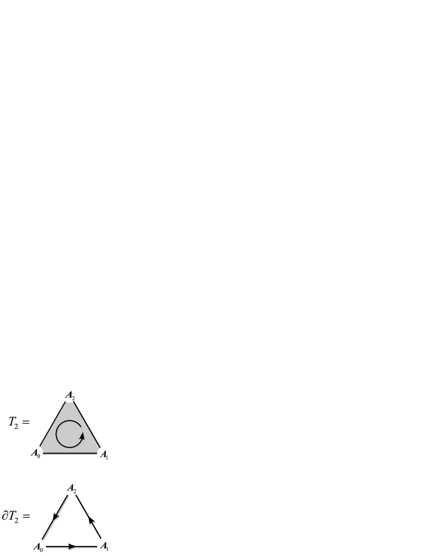
Figure 1: Connection structure associated to the simplex vertices.

With the preceding notation, the ECHF reads Man85

$$\int_{\partial T_{r+1}}\frac{l_{t}^{p}}{p!}\pi =\int_{T_{r+1}}\frac{l_{t}^{p+1}}{\left(p+1\right)!}\text{d}\pi+$$

$$+\left(-1\right)^{p+q}\text{d}\int_{T_{r+1}}\frac{l_{t}^{p+1}}{\left(p+1\right)!}\pi.$$ (53)

Here $\pi$ represents a polynomial in the forms $\left\{\bm{A}_{t},\bm{F}_{t},\text{d}_{t}\bm{A}_{t},\text{d}_{t}\bm{F}_{t}\right\}$ which is also an $m$-form on $M$ and a $q$-form on $T_{r+1}$, with $m\geq p$ and $p+q=r$. The exterior derivatives on $M$ and $T_{r+1}$ are denoted respectively by d and d_t. The operator $l_{t}$, called homotopy derivation, maps differential forms on $M$ and $T_{r+1}$ according to

$$l_{t}:\Omega^{a}\left(M\right)\times\Omega^{b}\left(T_{r+1}\right)\rightarrow\Omega^{a-1}\left(M\right)\times\Omega^{b+1}\left(T_{r+1}\right),$$ (54)

and it satisfies Leibniz’s rule as well as d and d_t. Its action on $\bm{A}_{t}$ and $\bm{F}_{t}$ reads Man85

$$l_{t}\bm{F}_{t} =\text{d}_{t}\bm{A}_{t},$$ (55)

$$l_{t}\bm{A}_{t} =0.$$ (56)

The three operators d, d_t and $l_{t}$ define a graded algebra given by

$$\text{d}^{2} =0,$$ (57)

$$\text{d}_{t}^{2} =0,$$ (58)

$$\left[l_{t},\text{d}\right] =\text{d}_{t},$$ (59)

$$\left[l_{t},\text{d}_{t}\right] =0,$$ (60)

$$\left\{\text{d},\text{d}_{t}\right\} =0.$$ (61)

Particular cases of (53), which we review below, reproduce both the Chern–Weil Theorem, eq. (7), and the Triangle Equation, eq. (47). In the rest of the paper we will always stick to the polynomial

$$\pi=\left\langle\bm{F}_{t}^{n+1}\right\rangle.$$ (62)

This choice has the three following properties: (i) $\pi$ is $M$-closed , i.e., d$\pi=0$, (ii) $\pi$ is a 0-form on $T_{r+1}$, i.e., $q=0$ and (iii) $\pi$ is a $\left(2n+2\right)$-form on $M$, i.e., $m=2n+2$. The allowed values for $p$ are $p=0,\ldots,2n+2$. The ECHF reduces in this case to

$$\int_{\partial T_{p+1}}\frac{l_{t}^{p}}{p!}\left\langle\bm{F}_{t}^{n+1}\right\rangle=\left(-1\right)^{p}\text{d}\int_{T_{p+1}}\frac{l_{t}^{p+1}}{\left(p+1\right)!}\left\langle\bm{F}_{t}^{n+1}\right\rangle.$$ (63)

We call eq. (63) the ‘restricted’ (or ‘closed’) version of the ECHF.

V.1 $p=0$: Chern–Weil Theorem

In this section we study the case $p=0$ of eq. (63),

$$\int_{\partial T_{1}}\left\langle\bm{F}_{t}^{n+1}\right\rangle=\text{d}\int_{T_{1}}l_{t}\left\langle\bm{F}_{t}^{n+1}\right\rangle,$$ (64)

where we must remember that $\bm{F}_{t}$ is the curvature tensor for the connection

$$\bm{A}_{t}=t^{0}\bm{A}_{0}+t^{1}\bm{A}_{1},$$ (65)

with $t^{0}$ and $t^{1}$ satisfying the constraint [cf. eq. (50)]

$$t^{0}+t^{1}=1.$$ (66)

The boundary of the simplex $T_{1}=\left(\bm{A}_{0}\bm{A}_{1}\right)$ is just

$$\partial\left(\bm{A}_{0}\bm{A}_{1}\right)=\left(\bm{A}_{1}\right)-\left(\bm{A}_{0}\right),$$ (67)

so that integration of the LHS of (64) is trivial:

$$\int_{\partial T_{1}}\left\langle\bm{F}_{t}^{n+1}\right\rangle=\left\langle\bm{F}_{1}^{n+1}\right\rangle-\left\langle\bm{F}_{0}^{n+1}\right\rangle.$$ (68)

On the other hand, the symmetric nature of $\left\langle\bm{F}_{t}^{n+1}\right\rangle$ implies that

$$l_{t}\left\langle\bm{F}_{t}^{n+1}\right\rangle=\left(n+1\right)\left\langle l_{t}\bm{F}_{t}\bm{F}_{t}^{n}\right\rangle.$$ (69)

Replacing $t^{0}=1-t^{1}$ we may write [cf. eq. (55)]

$$l_{t}\bm{F}_{t}=\text{d}_{t}\bm{A}_{t}=\text{d}t^{1}\left(\bm{A}_{1}-\bm{A}_{0}\right).$$ (70)

Since integration on $T_{1}$ actually corresponds to integrating with $t^{1}$ from $t^{1}=0$ to $t^{1}=1$, eq. (64) finally becomes

$$\left\langle\bm{F}_{1}^{n+1}\right\rangle-\left\langle\bm{F}_{0}^{n+1}\right\rangle=\text{d}Q_{\bm{A}_{1}\leftarrow\bm{A}_{0}}^{\left(2n+1\right)},$$ (71)

where the transgression form $Q_{\bm{A}_{1}\leftarrow\bm{A}_{0}}^{\left(2n+1\right)}$ is defined as

$$Q_{\bm{A}_{1}\leftarrow\bm{A}_{0}}^{\left(2n+1\right)} \equiv\int_{T_{1}}l_{t}\left\langle\bm{F}_{t}^{n+1}\right\rangle$$

$$=\left(n+1\right)\int_{0}^{1}\text{d}t\left\langle\left(\bm{A}_{1}-\bm{A}_{0}\right)\bm{F}_{t}^{n}\right\rangle.$$ (72)

This concludes our derivation of the Chern–Weil Theorem as a corollary of the ECHF.

V.2 $p=1$: Triangle Equation

In this section we study the case $p=1$ of eq. (63),

$$\int_{\partial T_{2}}l_{t}\left\langle\bm{F}_{t}^{n+1}\right\rangle=-\text{d}\int_{T_{2}}\frac{l_{t}^{2}}{2}\left\langle\bm{F}_{t}^{n+1}\right\rangle,$$ (73)

where $\bm{F}_{t}$ is the curvature corresponding to the connection $\bm{A}_{t}=t^{0}\bm{A}_{0}+t^{1}\bm{A}_{1}+t^{2}\bm{A}_{2}$. The boundary of the simplex $T_{2}=\left(\bm{A}_{0}\bm{A}_{1}\bm{A}_{2}\right)$ may be written as the sum

$$\partial\left(\bm{A}_{0}\bm{A}_{1}\bm{A}_{2}\right)=\left(\bm{A}_{1}\bm{A}_{2}\right)-\left(\bm{A}_{0}\bm{A}_{2}\right)+\left(\bm{A}_{0}\bm{A}_{1}\right),$$ (74)

so that the integral in the LHS of (73) is decomposed as

$$\int_{\partial T_{2}}l_{t}\left\langle\bm{F}_{t}^{n+1}\right\rangle =\int_{\left(\bm{A}_{1}\bm{A}_{2}\right)}l_{t}\left\langle\bm{F}_{t}^{n+1}\right\rangle+$$

$$-\int_{\left(\bm{A}_{0}\bm{A}_{2}\right)}l_{t}\left\langle\bm{F}_{t}^{n+1}\right\rangle+\int_{\left(\bm{A}_{0}\bm{A}_{1}\right)}l_{t}\left\langle\bm{F}_{t}^{n+1}\right\rangle.$$

Each of the terms in this equation is what we called before a transgression form:

$$\int_{\partial T_{2}}l_{t}\left\langle\bm{F}_{t}^{n+1}\right\rangle=Q_{\bm{A}_{2}\leftarrow\bm{A}_{1}}^{\left(2n+1\right)}-Q_{\bm{A}_{2}\leftarrow\bm{A}_{0}}^{\left(2n+1\right)}+Q_{\bm{A}_{1}\leftarrow\bm{A}_{0}}^{\left(2n+1\right)}.$$ (75)

On the other hand, Leibniz’s rule for $l_{t}$ and eq. (55) imply that

$$\int_{T_{2}}\frac{l_{t}^{2}}{2}\left\langle\bm{F}_{t}^{n+1}\right\rangle=\frac{1}{2}n\left(n+1\right)\int_{T_{2}}\left\langle\left(\text{d}_{t}\bm{A}_{t}\right)^{2}\bm{F}_{t}^{n-1}\right\rangle.$$ (76)

Integrating over the simplex we get

$$\int_{T_{2}}\frac{l_{t}^{2}}{2}\left\langle\bm{F}_{t}^{n+1}\right\rangle=Q_{\bm{A}_{2}\leftarrow\bm{A}_{1}\leftarrow\bm{A}_{0}}^{\left(2n\right)},$$ (77)

where $Q_{\bm{A}_{2}\leftarrow\bm{A}_{1}\leftarrow\bm{A}_{0}}^{\left(2n\right)}$ is given by

$$Q_{\bm{A}_{2}\leftarrow\bm{A}_{1}\leftarrow\bm{A}_{0}}^{\left(2n\right)} \equiv n\left(n+1\right)\int_{0}^{1}dt\int_{0}^{t}ds$$

$$\left\langle\left(\bm{A}_{2}-\bm{A}_{1}\right)\left(\bm{A}_{1}-\bm{A}_{0}\right)\bm{F}_{t}^{n-1}\right\rangle.$$ (78)

In (78) we have introduced dummy parameters $t=1-t^{0}$ and $s=t^{2}$, in terms of which $\bm{A}_{t}$ reads

$$\bm{A}_{t}=\bm{A}_{0}+t\left(\bm{A}_{1}-\bm{A}_{0}\right)+s\left(\bm{A}_{2}-\bm{A}_{1}\right).$$ (79)

Putting everything together, we find the Triangle Equation

$$Q_{\bm{A}_{2}\leftarrow\bm{A}_{1}}^{\left(2n+1\right)}-Q_{\bm{A}_{2}\leftarrow\bm{A}_{0}}^{\left(2n+1\right)}+Q_{\bm{A}_{1}\leftarrow\bm{A}_{0}}^{\left(2n+1\right)}=-\text{d}Q_{\bm{A}_{2}\leftarrow\bm{A}_{1}\leftarrow\bm{A}_{0}}^{\left(2n\right)},$$ (80)

or alternatively

$$Q_{\bm{A}_{2}\leftarrow\bm{A}_{0}}^{\left(2n+1\right)}=Q_{\bm{A}_{2}\leftarrow\bm{A}_{1}}^{\left(2n+1\right)}+Q_{\bm{A}_{1}\leftarrow\bm{A}_{0}}^{\left(2n+1\right)}+\text{d}Q_{\bm{A}_{2}\leftarrow\bm{A}_{1}\leftarrow\bm{A}_{0}}^{\left(2n\right)}.$$ (81)

We would like to stress here that use of the ECHF has now allowed us to pinpoint the exact form of the boundary contribution $Q_{\bm{A}_{2}\leftarrow\bm{A}_{1}\leftarrow\bm{A}_{0}}^{\left(2n\right)}$, eq. (78).

VI Subspace Separation Method for TGFT, with Two Examples

Our separation method is based on the Triangle Equation (81), and embodies the following steps:

1. Identify the relevant subspaces present in the gauge algebra, i.e., write $\mathfrak{g}=V_{0}\oplus\cdots\oplus V_{p}$.

2. Write the connections as a sum of pieces valued on every subspace, i.e., $\bm{A}=\bm{a}_{0}+\cdots+\bm{a}_{p}$, $\bar{\bm{A}}=\bar{\bm{a}}_{0}+\cdots+\bar{\bm{a}}_{p}$.

3. Use eq. (81) with

   $$\bm{A}_{0} =\bar{\bm{A}},$$ (82)

   $$\bm{A}_{1} =\bm{a}_{0}+\cdots+\bm{a}_{p-1},$$ (83)

   $$\bm{A}_{2} =\bm{A}.$$ (84)

4. Repeat step 3 for the transgression $Q_{\bm{A}_{1}\leftarrow\bm{A}_{0}}$, etc.

After performing these steps, one ends up with an equivalent expression for the TGFT lagrangian which has been separated in two different ways. First, the lagrangian is split into bulk and boundary contributions. This is due to the fact that each use of eq. (81) brings in a new boundary term. Second, each term in the bulk lagrangian refers to a different subspace of the gauge algebra. This comes about because the difference $\bm{A}_{2}-\bm{A}_{1}$ is valued only on one particular subspace.

Below we show two examples of TGFTs, one for Gravity and one for SUGRA. In both cases the separation method is used to cast the lagrangian in a physically sensible, readable way.

VI.1 Finite Action Principle for Gravity

In this section we aim to show explicitly how the lagrangian for gravity in $d=2n+1$ given in Mor04 corresponds to a transgression form for the connections

$$\bm{A}_{0} =\bar{\bm{\omega}},$$ (85)

$$\bm{A}_{2} =\bm{e}+\bm{\omega}.$$ (86)

Here we use the abbreviations $\bm{e}=e^{a}\bm{P}_{a}$, $\bm{\omega}=\frac{1}{2}\omega^{ab}\bm{J}_{ab}$, $\bar{\bm{\omega}}=\frac{1}{2}\bar{\omega}^{ab}\bm{J}_{ab}$, with $\bm{P}_{a},\bm{J}_{ab}$ being the generators of the AdS Algebra $\mathfrak{so}\left(2n,2\right)$. The curvatures for these connections read

$$\bm{F}_{0} =\bar{\bm{R}},$$ (87)

$$\bm{F}_{2} =\bm{R}+\bm{e}^{2}+\bm{T},$$ (88)

where

$$\bm{R} =\text{d}\bm{\omega}+\bm{\omega}^{2},$$ (89)

$$\bm{T} =\text{d}\bm{e}+\left[\bm{\omega},\bm{e}\right],$$ (90)

are the Lorentz curvature and the torsion, respectively [an expression completely analogous to (89) is valid for $\bar{\bm{R}}$].

As an invariant polynomial for the AdS Algebra we shall stick to our previous choice of the Levi-Civita tensor [cf. eq. (36)],

$$\left\langle\bm{J}_{a_{1}a_{2}}\cdots\bm{J}_{a_{2n-1}a_{2n}}\bm{P}_{a_{2n+1}}\right\rangle=\frac{2^{n}}{\ell}\varepsilon_{a_{1}\cdots a_{2n+1}},$$ (91)

with all other possible combinations vanishing.

In order to separate the pieces of our TGFT lagrangian in a meaningful way, we introduce the intermediate connection

$$\bm{A}_{1}=\bm{\omega}$$ (92)

and consider the Triangle Equation (81) as follows:

$$L_{\bm{e}+\bm{\omega}\leftarrow\bar{\bm{\omega}}}^{\left(2n+1\right)}=L_{\bm{e}+\bm{\omega}\leftarrow\bm{\omega}}^{\left(2n+1\right)}+kQ_{\bm{\omega}\leftarrow\bar{\bm{\omega}}}^{\left(2n+1\right)}+k\text{d}Q_{\bm{e}+\bm{\omega}\leftarrow\bm{\omega}\leftarrow\bar{\bm{\omega}}}^{\left(2n\right)}.$$ (93)

From section IV we know that the first term in the RHS of (93) corresponds to a LL lagrangian with the canonical coefficients [cf. eq. (39)],

$$L_{\bm{e}+\bm{\omega}\leftarrow\bm{\omega}}^{\left(2n+1\right)}=\left(n+1\right)k\int_{0}^{1}dt\left\langle\bm{eF}_{t}^{n}\right\rangle,$$ (94)

with $\bm{F}_{t}$ being the curvature for the connection $\bm{A}_{t}=\bm{\omega}+t\bm{e}$,$\ \bm{F}_{t}=\bm{R}+t\bm{T}+t^{2}\bm{e}^{2}$.

Our particular choice for the invariant polynomial now implies that the second term in (93) vanishes:

$$Q_{\bm{\omega}\leftarrow\bar{\bm{\omega}}}^{\left(2n+1\right)}=0.$$ (95)

Going back to eq. (78) we find that the boundary contribution in (93) may be written as

$$Q_{\bm{e}+\bm{\omega}\leftarrow\bm{\omega}\leftarrow\bar{\bm{\omega}}}^{\left(2n\right)}=n\left(n+1\right)\int_{0}^{1}dt\int_{0}^{t}ds\left\langle\bm{e\theta F}_{st}^{n-1}\right\rangle,$$ (96)

where

$$\bm{\theta}\equiv\bm{\omega}-\bar{\bm{\omega}}$$ (97)

and$\ \bm{F}_{st}$ is the curvature  for the connection $\bm{A}_{st}=\bar{\bm{\omega}}+s\bm{e}+t\bm{\theta}$,

$$\bm{F}_{st}=\bar{\bm{R}}+\text{D}_{\bar{\bm{\omega}}}\left(s\bm{e}+t\bm{\theta}\right)+s^{2}\bm{e}^{2}+st\left[\bm{e},\bm{\theta}\right]+t^{2}\bm{\theta}^{2}.$$ (98)

Putting everything together, our final lagrangian reads

$$L_{\bm{e}+\bm{\omega}\leftarrow\bar{\bm{\omega}}}^{\left(2n+1\right)} =\left(n+1\right)k\int_{0}^{1}dt\left\langle\bm{e}\left(\bm{R}+t^{2}\bm{e}^{2}\right)^{n}\right\rangle+$$

$$+k\text{d}Q_{\bm{e}+\bm{\omega}\leftarrow\bm{\omega}\leftarrow\bar{\bm{\omega}}}^{\left(2n\right)}.$$ (99)

The field equations for (99) are given by

$$\left\langle\bm{J}_{ab}\left(\bm{R}+\bm{e}^{2}\right)^{n-1}\bm{T}\right\rangle =0,$$ (100)

$$\left\langle\bm{P}_{a}\left(\bm{R}+\bm{e}^{2}\right)^{n}\right\rangle =0.$$ (101)

These can be obtained by direct variation of (99) or by replacing $\bm{F}_{0}$ and $\bm{F}_{2}$ in (18)–(19). A more explicit version is found making use of (91):

$$0 =\varepsilon_{aba_{1}\cdots a_{2n-1}}\left(R^{a_{1}a_{2}}+\frac{1}{\ell^{2}}e^{a_{1}}e^{a_{2}}\right)\times\cdots\times$$

$$\times\left(R^{a_{2n-3}a_{2n-2}}+\frac{1}{\ell^{2}}e^{a_{2n-3}}e^{a_{2n-2}}\right)T^{a_{2n-1}},$$ (102)

$$0 =\varepsilon_{aa_{1}\cdots a_{2n}}\left(R^{a_{1}a_{2}}+\frac{1}{\ell^{2}}e^{a_{1}}e^{a_{2}}\right)\times$$

$$\times\cdots\times\left(R^{a_{2n-1}a_{2n}}+\frac{1}{\ell^{2}}e^{a_{2n-1}}e^{a_{2n}}\right).$$ (103)

We have again two choices for obtaining boundary conditions; by direct variation of (99) or by replacing the relevant quantities in our general formula, eq. (20). Any of them can be shown to yield

$$\left.\int_{0}^{1}dt\left\langle\left(\delta\bar{\bm{\omega}}+t\delta\bm{\theta}+t\delta\bm{e}\right)\left(\bm{\theta}+\bm{e}\right)\bm{F}_{t}^{n-1}\right\rangle\right|_{\partial M}=0,$$ (104)

where in this case the connection $\bm{A}_{t}$ and the corresponding curvature $\bm{F}_{t}$ are given by

$$\bm{A}_{t} =\bar{\bm{\omega}}+t\left(\bm{e}+\bm{\theta}\right),$$ (105)

$$\bm{F}_{t} =\bar{\bm{R}}+t\text{D}_{\bar{\bm{\omega}}}\left(\bm{e}+\bm{\theta}\right)+t^{2}\left(\bm{e}^{2}+\left[\bm{e},\bm{\theta}\right]+\bm{\theta}^{2}\right).$$ (106)

There are many alternative ways of satisfying boundary conditions (104). In Mor04 , physical arguments  are given that allow to partially fix the boundary conditions; perhaps the most significant of them is demanding that $\bar{\bm{\omega}}$ have a fixed value on $\partial M$, i.e.,

$$\left.\delta\bar{\bm{\omega}}\right|_{\partial M}=0.$$ (107)

The remaining boundary conditions may be written as

$$\left.\int_{0}^{1}dt\left\langle t\left(\delta\bm{\theta e}-\bm{\theta}\delta\bm{e}\right)\left(\bar{\bm{R}}+t^{2}\bm{e}^{2}+t^{2}\bm{\theta}^{2}\right)^{n-1}\right\rangle\right|_{\partial M}=0,$$ (108)

and can be readily satisfied by requiring

$$\delta\theta^{[ab}e^{c]}=\theta^{[ab}\delta e^{c]}.$$ (109)

We would like to stress that the choice (91) for the invariant polynomial sends all dependence on $\bar{\bm{\omega}}$ in the action to a boundary term, and in this way the potential conflict of having two independent CS theories living on the same space-time manifold is avoided. The presence of $\bar{\bm{\omega}}$ in the lagrangian does nevertheless have a dramatic effect on the theory, as it changes the boundary conditions and renders both the TGFT action and the conserved charges finite . Further important theoretical implications are examined in section VII.

VI.2 Supergravity as a TGFT

The move from standard CS Theory to TGFT earns us several important advantages, both in computational power and in theoretical clarity. The latter will be thoroughly discussed in section VII; here we shall be mainly concerned with elaborating on the former.

One first disadvantage of the standard CS action formula surfaces when one wants to perform the separation of the lagrangian in reflection of the subspaces structure of the gauge algebra. As a matter of fact, it is clear from the very nature of a CS form that this will require intensive use of Leibniz’s rule, which, especially for complicated algebras in dimensions higher than three, renders the task a highly non-trivial ‘artistic’ work.

These manipulations finally lead to a separation of the CS lagrangian in bulk and boundary contributions. After performing this separation, it is no longer clear whether one should simply drop these boundary terms, since the bulk lagrangian is still invariant under infinitesimal gauge transformations (up to a total derivative). Even more involved is the derivation of boundary conditions from the CS lagrangian; on one hand, they’re, from a purely computational point of view, rather difficult to extract, and on the other, they of course depend on our earlier choice of dropping or not the boundary contributions just obtained.

On the other hand, the TGFT lagrangian clearly distinguishes itself from a CS lagrangian in this respect. As a matter of fact, the separation method sketched at the beginning of section VI applied to the TGFT lagrangian permits the straightforward realization of both tasks. The lagrangian is split into bulk and boundary contributions, and the bulk sector is divided into pieces that faithfully reflect the subspace structure of the gauge algebra. Furthermore, the boundary conditions arising from these boundary terms have a chance to be physically meaningful, due to the full invariance of the TGFT lagrangian under gauge transformations.

In order to highlight the way in which the TGFT formalism deals with these issues, we present here the TGFT derivation of a CS SUGRA lagrangian. For a non-trivial example we pick $d=5$ and choose the $\mathcal{N}$-extended AdS superalgebra $\mathfrak{u}\left(4|\mathcal{N}\right)$ (see Refs. Cha90 ; Tro96 ; Tro98 ). This algebra is generated by the set $\left\{\bm{K},\bm{P}_{a},\bm{J}_{ab},\bm{M}_{n}^{\;m},\bm{Q}_{i}^{\alpha},\bar{\bm{Q}}_{\alpha}^{i}\right\}$. Latin letters from the beginning of the alphabet $\left(a,b,c,\ldots\right)$ denote Lorentz indices and rank from 0 to 4; Greek letters $\left(\alpha,\beta,\gamma,\ldots\right)$ denote spinor indices and rank from 1 to 4 (the dimension of a Dirac spinor in $d=5$ is $2^{\left[5/2\right]}=4$); Latin letters from the middle of the alphabet $\left(i,j,k,\ldots\right)$ denote $\mathfrak{su}\left(\mathcal{N}\right)$ indices, which rank from 1 to $\mathcal{N}$ and can be regarded as ‘counting’ fermionic generators. The non-vanishing (anti)commutation relations read

$$\left[\bm{K},\bm{Q}_{k}^{\alpha}\right] =-i\left(\frac{1}{4}-\frac{1}{\mathcal{N}}\right)\bm{Q}_{k}^{\alpha},$$ (110)

$$\left[\bm{M}_{k}^{\;j},\bm{Q}_{m}^{\alpha}\right] =\left(\delta_{k}^{p}\delta_{m}^{j}-\frac{1}{\mathcal{N}}\delta_{m}^{p}\delta_{k}^{j}\right)\bm{Q}_{p}^{\alpha},$$ (111)

$$\left[\bm{P}_{a},\bm{Q}_{k}^{\alpha}\right] =-\frac{1}{2\ell}\left(\Gamma_{a}\right)_{\;\beta}^{\alpha}\bm{Q}_{k}^{\beta},$$ (112)

$$\left[\bm{J}_{ab},\bm{Q}_{k}^{\alpha}\right] =-\frac{1}{2}\left(\Gamma_{ab}\right)_{\;\beta}^{\alpha}\bm{Q}_{k}^{\beta},$$ (113)

$$\left[\bm{M}_{k}^{\;j},\bm{M}_{m}^{\;l}\right]=\delta_{m}^{j}\bm{M}_{k}^{\;l}-\delta_{k}^{l}\bm{M}_{m}^{\;j},$$ (114)

$$\left\{\bm{Q}_{k}^{\alpha},\bar{\bm{Q}}_{\beta}^{j}\right\} =2\delta_{k}^{j}\left(\Gamma^{a}\right)_{\;\beta}^{\alpha}\bm{P}_{a}+$$

$$-\frac{4}{\ell}\left[i\delta_{k}^{j}\delta_{\beta}^{\alpha}\bm{K}-\delta_{\beta}^{\alpha}\bm{M}_{k}^{\;j}+\frac{1}{4}\delta_{k}^{j}\left(\Gamma^{ab}\right)_{\;\beta}^{\alpha}\bm{J}_{ab}\right],$$ (115)

where $\Gamma_{a}$ are Dirac Matrices  in $d=5$ and $\Gamma_{ab}\equiv\frac{1}{2}\left[\Gamma_{a},\Gamma_{b}\right]$. The generators $\bm{M}_{k}^{\;j}$ span an $\mathfrak{su}\left(\mathcal{N}\right)$ subalgebra, while $\bm{P}_{a}$ and $\bm{J}_{ab}$ generate as usual the AdS algebra [omitted above, see (32)–(34)]. The anticommutator $\left\{\bm{Q},\bar{\bm{Q}}\right\}$ has components on all bosonic generators, and not only on the translational ones. This is a consequence of the fact that we are considering the supersymmetric version of the AdS Algebra, as opposed to the Poincaré Algebra. The latter may be recovered via an İnönü–Wigner contraction by setting $\ell\rightarrow\infty$ [in which case only the translational part in the RHS of (115) survives]. Commutators of the form $\left[\bm{B},\bar{\bm{Q}}\right]$, where $\bm{B}$ is some bosonic generator, differ only by a sign from their $\left[\bm{B},\bm{Q}\right]$ counterparts and have not been explicitly written out. For $\mathcal{N}=4$ the generator $\bm{K}$ becomes abelian and factors out from the rest of the algebra.

The second ingredient we need in order to write down the TGFT lagrangian is a $\mathfrak{u}\left(4|\mathcal{N}\right)$-invariant symmetric polynomial $\left\langle\cdots\right\rangle$ of rank three. This can be conveniently defined as the supersymmetrized supertrace of the product of three supermatrices representing as many generators in $\mathfrak{u}\left(4|\mathcal{N}\right)$. The fact that the Dirac Matrices provide a natural representation for the AdS Algebra is a turning point that makes this construction feasible. Without going into the details, the invariant polynomial we will use satisfies the following contraction identities:

$$\left\langle\bm{K}^{3}\right\rangle = \frac{1}{4^{2}}-\frac{1}{\mathcal{N}^{2}},$$ (116)

$$B_{\;n}^{m}C_{\;q}^{p}\left\langle\bm{KM}_{m}^{\;n}\bm{M}_{p}^{\;q}\right\rangle = \frac{1}{\mathcal{N}}B_{\;p}^{q}C_{\;q}^{p},$$ (117)

$$B^{a}C^{b}\left\langle\bm{KP}_{a}\bm{P}_{b}\right\rangle = -\frac{1}{4\ell^{2}}B^{a}C_{a},$$ (118)

$$B^{ab}C^{cd}\left\langle\bm{KJ}_{ab}\bm{J}_{cd}\right\rangle = -\frac{1}{2}B_{\;b}^{a}C_{\;a}^{b},$$ (119)

$$A_{\;n}^{m}B_{\;q}^{p}B_{\;s}^{r}\left\langle\bm{M}_{m}^{\;n}\bm{M}_{p}^{\;q}\bm{M}_{r}^{\;s}\right\rangle =-iA_{\;p}^{m}B_{\;q}^{p}B_{\;m}^{q},$$ (120)

$$A^{a}B^{bc}C^{de}\left\langle\bm{P}_{a}\bm{J}_{bc}\bm{J}_{de}\right\rangle =-\frac{\gamma}{2\ell}\varepsilon_{abcde}A^{a}B^{bc}C^{de},$$ (121)

$$\bar{\zeta}^{m}B\chi_{n}\left\langle\bm{Q}_{m}\bm{K}\bar{\bm{Q}}^{n}\right\rangle = \frac{2}{\ell}\left(\frac{1}{4}+\frac{1}{\mathcal{N}}\right)\bar{\zeta}B\chi,$$ (122)

$$\bar{\zeta}^{m}B^{a}\chi_{n}\left\langle\bm{Q}_{m}\bm{J}_{a}\bar{\bm{Q}}^{n}\right\rangle = -\frac{i}{\ell}\bar{\zeta}B^{a}\Gamma_{a}\chi,$$ (123)

$$\bar{\zeta}^{m}B^{ab}\chi_{n}\left\langle\bm{Q}_{m}\bm{J}_{ab}\bar{\bm{Q}}^{n}\right\rangle = -\frac{i}{\ell}\bar{\zeta}B^{ab}\Gamma_{ab}\chi,$$ (124)

$$\bar{\zeta}^{p}B_{\;n}^{m}\chi_{q}\left\langle\bm{Q}_{p}\bm{M}_{m}^{\;n}\bar{\bm{Q}}^{q}\right\rangle = -\frac{2i}{\ell}\bar{\zeta}^{n}B_{\;n}^{m}\chi_{m}.$$ (125)

Here $A,B,C,\zeta,\chi$ are arbitrary differential forms with appropriate index structure . It is interesting to note that the invariant polynomial used in section VI.1 is recovered unchanged (but for a different overall factor) in eq. (121).

We will choose as lagrangian the transgression form that interpolates between the following connections:

$$\bm{A}_{0} =\bar{\bm{\omega}},$$ (126)

$$\bm{A}_{4} =\bm{e}+\bm{\omega}+\bm{b}+\bm{a}+\bar{\bm{\psi}}-\bm{\psi},$$ (127)

where

$$\bm{e} =e^{a}\bm{P}_{a},$$ (128)

$$\bm{\omega} =\frac{1}{2}\omega^{ab}\bm{J}_{ab},$$ (129)

$$\bar{\bm{\omega}} =\frac{1}{2}\bar{\omega}^{ab}\bm{J}_{ab},$$ (130)

$$\bm{b} =b\bm{K},$$ (131)

$$\bm{a} =a_{\;n}^{m}\bm{M}_{m}^{\;n},$$ (132)

$$\bar{\bm{\psi}} =\bar{\psi}\bm{Q},$$ (133)

$$\bm{\psi} =\bar{\bm{Q}}\psi.$$ (134)

The corresponding curvatures read

$$\bm{F}_{0}=\bar{\bm{R}},$$ (135)

$$\bm{F}_{4}=\left(\text{d}b+\frac{i}{\ell}\bar{\psi}\psi\right)\bm{K}+\bm{f}^{\prime}+\bm{T}^{\prime}+\bm{R}^{\prime}+\frac{1}{2}\left(\nabla\bar{\psi}\bm{Q}-\bar{\bm{Q}}\nabla\psi\right),$$ (136)

where we have defined

$$\bm{f} =\text{d}\bm{a}+\bm{a}^{2},$$ (137)

$$\bm{f}^{\prime} =\bm{f}-\frac{1}{\ell}\left(\bar{\psi}^{m}\psi_{n}\right)\bm{M}_{m}^{\;n},$$ (138)

$$\bm{T}^{\prime} =\bm{T}-\frac{1}{2}\left(\bar{\psi}\Gamma^{a}\psi\right)\bm{P}_{a},$$ (139)

$$\bm{R}^{\prime} =\bm{R}+\bm{e}^{2}+\frac{1}{4\ell}\left(\bar{\psi}\Gamma^{ab}\psi\right)\bm{J}_{ab},$$ (140)

and

$$\nabla\psi_{k} \equiv\text{d}\psi_{k}+\frac{1}{2\ell}e^{a}\Gamma_{a}\psi_{k}+\frac{1}{4}\omega^{ab}\Gamma_{ab}\psi_{k}+$$

$$-a_{\;k}^{l}\psi_{l}+i\left(\frac{1}{4}-\frac{1}{\mathcal{N}}\right)b\psi_{k},$$ (141)

$$\nabla\bar{\psi}^{k} \equiv\text{d}\bar{\psi}^{k}-\frac{1}{2\ell}e^{a}\bar{\psi}^{k}\Gamma_{a}-\frac{1}{4}\omega^{ab}\bar{\psi}^{k}\Gamma_{ab}+$$

$$+a_{\;l}^{k}\bar{\psi}^{l}-i\left(\frac{1}{4}-\frac{1}{\mathcal{N}}\right)b\bar{\psi}^{k}.$$ (142)

We thus have

$$L_{\text{sugra}}^{\left(5\right)} =kQ_{\bm{A}_{4}\leftarrow\bm{A}_{0}}^{\left(5\right)},$$

$$=3k\int_{0}^{1}dt\left\langle\bm{\Theta F}_{t}^{2}\right\rangle,$$ (143)

with

$$\bm{\theta} =\bm{\omega}-\bar{\bm{\omega}},$$ (144)

$$\bm{\Theta} =\bm{e}+\bm{\theta}+\bm{b}+\bm{a}+\bar{\bm{\psi}}-\bm{\psi},$$ (145)

and $\bm{F}_{t}$ being the curvature for the connection

$$\bm{A}_{t}=\bar{\bm{\omega}}+t\left(\bm{e}+\bm{\theta}+\bm{b}+\bm{a}+\bar{\bm{\psi}}-\bm{\psi}\right).$$ (146)

In order to make sense of (143) we introduce the following set of intermediate connections:

$$\bm{A}_{1} =\bm{e}+\bm{\omega},$$ (147)

$$\bm{A}_{2} =\bm{e}+\bm{\omega}+\bm{b},$$ (148)

$$\bm{A}_{3} =\bm{e}+\bm{\omega}+\bm{b}+\bm{a}.$$ (149)

Now we split $Q_{\bm{A}_{4}\leftarrow\bm{A}_{0}}^{\left(5\right)}$ according to the pattern 

$$Q_{\bm{A}_{4}\leftarrow\bm{A}_{0}}^{\left(5\right)} =Q_{\bm{A}_{4}\leftarrow\bm{A}_{3}}^{\left(5\right)}+Q_{\bm{A}_{3}\leftarrow\bm{A}_{0}}^{\left(5\right)}+\text{d}Q_{\bm{A}_{4}\leftarrow\bm{A}_{3}\leftarrow\bm{A}_{0}}^{\left(4\right)},$$ (150)

$$Q_{\bm{A}_{3}\leftarrow\bm{A}_{0}}^{\left(5\right)} =Q_{\bm{A}_{3}\leftarrow\bm{A}_{2}}^{\left(5\right)}+Q_{\bm{A}_{2}\leftarrow\bm{A}_{0}}^{\left(5\right)}+\text{d}Q_{\bm{A}_{3}\leftarrow\bm{A}_{2}\leftarrow\bm{A}_{0}}^{\left(4\right)},$$ (151)

$$Q_{\bm{A}_{2}\leftarrow\bm{A}_{0}}^{\left(5\right)} =Q_{\bm{A}_{2}\leftarrow\bm{A}_{1}}^{\left(5\right)}+Q_{\bm{A}_{1}\leftarrow\bm{A}_{0}}^{\left(5\right)}+\text{d}Q_{\bm{A}_{2}\leftarrow\bm{A}_{1}\leftarrow\bm{A}_{0}}^{\left(4\right)}.$$ (152)

Picking up the pieces, we are left with

$$L_{\text{sugra}}^{\left(5\right)}=L_{\bm{\psi}}^{\left(5\right)}+L_{\bm{a}}^{\left(5\right)}+L_{\bm{b}}^{\left(5\right)}+L_{\bm{e}+\bm{\omega}\leftarrow\bar{\bm{\omega}}}^{\left(5\right)}+\text{d}B_{\text{sugra}}^{\left(4\right)},$$ (153)

where we have defined

$$L_{\bm{\psi}}^{\left(5\right)} \equiv kQ_{\bm{A}_{4}\leftarrow\bm{A}_{3}}^{\left(5\right)},$$ (154)

$$L_{\bm{a}}^{\left(5\right)} \equiv kQ_{\bm{A}_{3}\leftarrow\bm{A}_{2}}^{\left(5\right)},$$ (155)

$$L_{\bm{b}}^{\left(5\right)} \equiv kQ_{\bm{A}_{2}\leftarrow\bm{A}_{1}}^{\left(5\right)},$$ (156)

$$L_{\bm{e}+\bm{\omega}\leftarrow\bar{\bm{\omega}}}^{\left(5\right)} \equiv kQ_{\bm{A}_{1}\leftarrow\bm{A}_{0}}^{\left(5\right)},$$ (157)

$$B_{\text{sugra}}^{\left(4\right)}\equiv kQ_{\bm{A}_{2}\leftarrow\bm{A}_{1}\leftarrow\bm{A}_{0}}^{\left(4\right)}+kQ_{\bm{A}_{3}\leftarrow\bm{A}_{2}\leftarrow\bm{A}_{0}}^{\left(4\right)}+kQ_{\bm{A}_{4}\leftarrow\bm{A}_{3}\leftarrow\bm{A}_{0}}^{\left(4\right)}.$$ (158)

A few comments are in order. Ignoring for the moment the boundary contribution $B_{\text{sugra}}^{\left(4\right)}$, we see that all dependence on the fermions has been packaged in $L_{\bm{\psi}}^{\left(5\right)}$, which we call ‘fermionic lagrangian’. Similarly, $L_{\bm{a}}^{\left(5\right)}$ and $L_{\bm{b}}^{\left(5\right)}$ correspond to pieces that are highly dependent on $\bm{a}$ and $\bm{b}$ respectively, although some dependence on $\bm{a}$ and $\bm{b}$ is also found on $L_{\bm{\psi}}^{\left(5\right)}$. In turn, $L_{\bm{b}}^{\left(5\right)}$ carries no dependence on $\bm{a}$. The last piece, $L_{\bm{e}+\bm{\omega}\leftarrow\bar{\bm{\omega}}}^{\left(5\right)}$, is, thanks to the particular invariant polynomial used, exactly what we considered in section VI.1, and stands alone as the ‘gravity’ lagrangian. Explicit versions for every piece may be easily obtained by going back to the definition of a transgression form, eq. (8). As a matter of fact, a straightforward computation yields

$$L_{\bm{\psi}}^{\left(5\right)} =\frac{3k}{2i}\left(\bar{\psi}_{\alpha}\mathcal{R}_{\;\beta}^{\alpha}\nabla\psi^{\beta}+\bar{\psi}^{n}\mathcal{F}_{\;n}^{m}\nabla\psi_{m}+\right.$$

$$\left.-\nabla\bar{\psi}_{\alpha}\mathcal{R}_{\;\beta}^{\alpha}\psi^{\beta}-\nabla\bar{\psi}^{n}\mathcal{F}_{\;n}^{m}\psi_{m}\right),$$ (159)

$$L_{\bm{a}}^{\left(5\right)} =\frac{3k}{\mathcal{N}}\left(\text{d}b\right)\operatorname*{Tr}\left(a\text{d}a+\frac{2}{3}a^{3}\right)+$$

$$-ik\operatorname*{Tr}\left[a\left(\text{d}a\right)^{2}+\frac{3}{2}a^{3}\text{d}a+\frac{3}{5}a^{5}\right],$$ (160)

$$L_{\bm{b}}^{\left(5\right)} =k\left(\frac{1}{4^{2}}-\frac{1}{\mathcal{N}^{2}}\right)b\left(\text{d}b\right)^{2}+$$

$$-\frac{3k}{4\ell^{2}}b\left(T^{a}T_{a}-R_{ab}e^{a}e^{b}-\frac{\ell^{2}}{2}R^{ab}R_{ab}\right),$$ (161)

where

$$\mathcal{R}_{\;\beta}^{\alpha} =i\left(\frac{1}{4}+\frac{1}{\mathcal{N}}\right)\left(\text{d}b+\frac{i}{2\ell}\bar{\psi}\psi\right)\delta_{\beta}^{\alpha}+$$

$$+\frac{1}{2}\left(T^{a}-\frac{1}{4}\bar{\psi}\Gamma^{a}\psi\right)\left(\Gamma_{a}\right)_{\;\beta}^{\alpha}+$$

$$+\frac{1}{4}\left(R^{ab}+\frac{1}{\ell^{2}}e^{a}e^{b}+\frac{1}{4\ell}\bar{\psi}\Gamma^{ab}\psi\right)\left(\Gamma_{ab}\right)_{\;\beta}^{\alpha},$$ (162)

$$\mathcal{F}_{\;n}^{m}=f_{\;n}^{m}-\frac{1}{2\ell}\bar{\psi}^{m}\psi_{n}.$$ (163)

The lagrangian for the $\mathfrak{su}\left(\mathcal{N}\right)$ field $\bm{a}$ includes both a CS term for $d=5$ and a CS term for $d=3$, the latter being suitable multiplied by the field-strength for the $\bm{b}$-field, d$b$.

The equations of motion and the boundary conditions are easily obtained using the general expressions (18)–(20). These are natural extensions of (100)–(101) and are also found in Tro98 .

We would like to stress the fact that the preceding results have been obtained in a completely straightforward way, without using Leibniz’s rule, following the method given in section VI. The same task can be painstakingly long if approached naïvely, i.e., through the sole use of Leibniz’s rule and the definition of a CS or TGFT lagrangian.

VII Discussion

VII.1 The Gauge-Theory Structure of TGFT Gravity

In the TGFT lagrangians for gravity, eqs. (39) and (99), one of the connections involved, namely $\omega$ or $\bar{\omega}$, is valued only on the Lorentz subalgebra of the full AdS algebra. Here we consider some implications of this fact.

Let us consider first the particular case of the Transgression form $Q_{\bm{\omega}+\bm{e}\leftarrow\bm{\omega}}^{\left(2n+1\right)}$ with the Levi-Civita tensor as $\mathfrak{so}\left(2n,2\right)$-invariant symmetric polynomial,

$$Q_{\bm{\omega}+\bm{e}\leftarrow\bm{\omega}}^{\left(2n+1\right)}=\left(n+1\right)\int_{0}^{1}dt\left\langle\bm{e}\left(\bm{R}+t^{2}\bm{e}^{2}\right)^{n}\right\rangle.$$ (164)

The RHS of eq. (164) has the remarkable feature of changing only by a total derivative  under the infinitesimal $\mathfrak{so}\left(2n,2\right)$ gauge transformations

$$\delta e^{a} =\lambda_{\;b}^{a}e^{b}-\text{D}_{\omega}\lambda^{a},$$ (165)

$$\delta\omega^{ab} =-\text{D}_{\omega}\lambda^{ab}-\frac{1}{\ell^{2}}\left(e^{a}\lambda^{b}-e^{b}\lambda^{a}\right).$$ (166)

This seems puzzling, because, as we saw in section III.2, a Transgression form in general should be fully invariant, with no additional terms appearing under gauge transformations. This behavior has its origin in the fact that the above transformations are gauge transformations for the connection $\bm{A}=\bm{\omega}+\bm{e}$, but not for the connection $\bar{\bm{A}}=\bm{\omega}$. Furthermore, it looks impossible to simultaneously define consistent gauge transformations for both connections $\bm{A}=\bm{\omega}+\bm{e}$ and $\bar{\bm{A}}=\bm{\omega}$.

Bearing this in mind, it now seems amazing that (164) changes only by a closed term under these ‘pathological’ gauge transformations! This puzzle is related with some interesting properties of the choice of invariant symmetric tensor.

In order to shed some light onto this riddle, let us consider the Transgression form $Q_{\bm{\omega}+\bm{e}\leftarrow\bm{\omega}}^{\left(2n+1\right)}$ with an arbitrary invariant symmetric tensor $\left\langle\cdots\right\rangle$. Then, from the Chern–Weil theorem, we know that

$$\left\langle\bm{F}^{n+1}\right\rangle-\left\langle\bm{R}^{n+1}\right\rangle=\text{d}Q_{\bm{\omega}+\bm{e}\leftarrow\bm{\omega}}^{\left(2n+1\right)},$$ (167)

where $\bm{F}$ and $\bm{R}$ are the curvatures for $\bm{\omega}+\bm{e}$ and $\bm{\omega}$, respectively.

Because the transformations (165)–(166) are gauge transformations for $\bm{A}=\bm{\omega}+\bm{e}$ but not for $\bar{\bm{A}}=\bm{\omega}$, $\bm{F}$ will change under them as an $\mathfrak{so}\left(2n,2\right)$-tensor, but $\bm{R}$ will not. Therefore, $\left\langle\bm{F}^{n+1}\right\rangle$ will stay invariant under (165)–(166) but not $\left\langle\bm{R}^{n+1}\right\rangle$. As a consequence, the LHS in (167) will be modified under these pathological gauge transformations, and then of course also the RHS. In general, $Q_{\bm{\omega}+\bm{e}\leftarrow\bm{\omega}}^{\left(2n+1\right)}$ is simply not invariant at all under these transformations.

But when the invariant symmetric polynomial is such that $\left\langle\bm{R}^{n+1}\right\rangle$ remains unchanged even under these non-gauge transformations, then $Q_{\bm{\omega}+\bm{e}\leftarrow\bm{\omega}}^{\left(2n+1\right)}$ can at most vary by a closed form under them. This is precisely the case for the choice of the Levi-Civita tensor. In this case, because $\left\langle\bm{J}_{a_{1}a_{2}}\cdots\bm{J}_{a_{2n+1}a_{2n+2}}\right\rangle=0$, we have $\left\langle\bm{R}^{n+1}\right\rangle=0$ and this value is not modified even under the ‘pathological’ gauge transformations.

It is interesting to notice how remarkable the invariant symmetric polynomial structure has been: it is also the reason why $Q_{\bm{\omega}+\bm{e}\leftarrow\bm{\omega}}^{\left(2n+1\right)}$ and the CS form differ only by a total derivative, and as we will see after some discussion, it has further importance.

Setting aside the suggestive fact that $Q_{\bm{\omega}+\bm{e}\leftarrow\bm{\omega}}^{\left(2n+1\right)}$ changes only by boundary contributions under the transformations, the mathematical beauty problem remains: those are not gauge transformations for our fields.

This problem has one clear solution: change the configuration of connections into another one better behaved. This is precisely what happens with the second expression used as Lagrangian, $Q_{\bm{\omega}+\bm{e}\leftarrow\bar{\bm{\omega}}}^{\left(2n+1\right)}$. On this expression it is possible to define in a consistent way simultaneous SO$\left(2n,2\right)$ gauge transformations over $\bm{A}=\bm{\omega}+\bm{e}$ and $\bar{\bm{A}}=\bm{\omega}$,

$$\delta\bm{A} =-\frac{1}{2}\left[\text{D}_{\omega}\lambda^{ab}+\frac{1}{\ell^{2}}\left(e^{a}\lambda^{b}-e^{b}\lambda^{a}\right)\right]\bm{J}_{ab}+$$

$$+\left(\lambda_{\;b}^{a}e^{b}-\text{D}_{\omega}\lambda^{a}\right)\bm{P}_{a},$$ (168)

$$\delta\bar{\bm{A}} =-\frac{1}{2}\text{D}_{\bar{\omega}}\lambda^{ab}\bm{J}_{ab}-\text{D}_{\bar{\omega}}\lambda^{a}\bm{P}_{a},$$ (169)

such that $Q_{\bm{\omega}+\bm{e}\leftarrow\bar{\bm{\omega}}}^{\left(2n+1\right)}$ stays fully invariant under them, as it should be.

Two intriguing facts appear now. The first of them is that the difference between $Q_{\bm{\omega}+\bm{e}\leftarrow\bar{\bm{\omega}}}^{\left(2n+1\right)}$ and $Q_{\bm{\omega}+\bm{e}\leftarrow\bm{\omega}}^{\left(2n+1\right)}$ is only a total derivative, and therefore it seems surprising that the gauge transformations are ill-defined over $Q_{\bm{\omega}+\bm{e}\leftarrow\bm{\omega}}^{\left(2n+1\right)}$, whereas there is no problem with $Q_{\bm{\omega}+\bm{e}\leftarrow\bar{\bm{\omega}}}^{\left(2n+1\right)}$. The second fact is that the statement that $\bar{\bm{A}}=\bar{\bm{\omega}}$ has components only on the Lorentz subalgebra is not a gauge-invariant one. As a matter of fact, an AdS boost on $\bar{\bm{A}}$ will generate a $\bm{P}_{a}$-piece: a ‘pure-gauge’ vielbein (see section VII.2).

The first of these facts finds a natural explanation in the context of the Triangle equation [cf. eq. (81)],

$$Q_{\bm{A}_{2}\leftarrow\bm{A}_{0}}^{\left(2n+1\right)}=Q_{\bm{A}_{2}\leftarrow\bm{A}_{1}}^{\left(2n+1\right)}+Q_{\bm{A}_{1}\leftarrow\bm{A}_{0}}^{\left(2n+1\right)}+\text{d}Q_{\bm{A}_{2}\leftarrow\bm{A}_{1}\leftarrow\bm{A}_{0}}^{\left(2n\right)}.$$ (170)

Here it suffices to notice that $Q_{\bm{A}_{2}\leftarrow\bm{A}_{0}}^{\left(2n+1\right)}$ does not depend on $\bm{A}_{1}$, and it remains invariant under any kind of transformation $\bm{A}_{1}\rightarrow\bm{A}_{1}^{\prime}$, even when this is not a gauge transformation.

For this reason, we can see that in the particular case $\bm{A}_{0}=\bar{\bm{\omega}}$, $\bm{A}_{1}=\bm{\omega}$, $\bm{A}_{2}=\bm{\omega}+\bm{e}$,

$$Q_{\bm{\omega}+\bm{e}\leftarrow\bar{\bm{\omega}}}^{\left(2n+1\right)}=Q_{\bm{\omega}+\bm{e}\leftarrow\bm{\omega}}^{\left(2n+1\right)}+Q_{\bm{\omega}\leftarrow\bar{\bm{\omega}}}^{\left(2n+1\right)}+\text{d}Q_{\bm{\omega}+\bm{e}\leftarrow\bm{\omega}\leftarrow\bar{\bm{\omega}}}^{\left(2n\right)},$$

the Transgression form $Q_{\bm{\omega}+\bm{e}\leftarrow\bar{\bm{\omega}}}^{\left(2n+1\right)}$ will stay fully invariant under the infinitesimal transformations

$$\delta\bm{A}_{0} =-\frac{1}{2}\text{D}_{\bar{\omega}}\lambda^{ab}\bm{J}_{ab}-\text{D}_{\bar{\omega}}\lambda^{a}\bm{P}_{a},$$ (171)

$$\delta\bm{A}_{1} =-\frac{1}{2}\left[\text{D}_{\omega}\lambda^{ab}+\frac{1}{\ell^{2}}\left(e^{a}\lambda^{b}-e^{b}\lambda^{a}\right)\right]\bm{J}_{ab},$$ (172)

$$\delta\bm{A}_{2} =-\frac{1}{2}\left[\text{D}_{\omega}\lambda^{ab}+\frac{1}{\ell^{2}}\left(e^{a}\lambda^{b}-e^{b}\lambda^{a}\right)\right]\bm{J}_{ab}+$$

$$+\left(\lambda_{\;b}^{a}e^{b}-\text{D}_{\omega}\lambda^{a}\right)\bm{P}_{a},$$ (173)

even though they do not correspond to a gauge transformation  for $\bm{A}_{1}$. The difference between the present case and the former is that $Q_{\bm{\omega}+\bm{e}\leftarrow\bar{\bm{\omega}}}^{\left(2n+1\right)}$ does not depend on $\bm{A}_{1}$ and therefore there’s no contradiction in having non-gauge transformation laws for it.

On the other hand, when the Levi-Civita symbol is chosen, then $Q_{\bm{\omega}\leftarrow\bar{\bm{\omega}}}^{\left(2n+1\right)}=0$ and we can write

$$Q_{\bm{\omega}+\bm{e}\leftarrow\bar{\bm{\omega}}}^{\left(2n+1\right)}=Q_{\bm{\omega}+\bm{e}\leftarrow\bm{\omega}}^{\left(2n+1\right)}+\text{d}Q_{\bm{\omega}+\bm{e}\leftarrow\bm{\omega}\leftarrow\bar{\bm{\omega}}}^{\left(2n\right)}.$$ (174)

VII.2 Locality vs. Globality

We would like to focus now our attention on a subtle and interesting fact related to eq. (174): its LHS has more information than its RHS. As matter of fact, under an $\mathfrak{so}\left(2n,2\right)$ gauge transformation, $\bm{A}_{0}=\bar{\bm{\omega}}$ changes as

$$\bm{A}_{0}=\bar{\bm{\omega}}\rightarrow\bm{A}_{0}^{\prime}=\bar{\bm{\omega}}^{\prime}+\bar{\bm{e}}_{\text{g}},$$ (175)

where $\bar{\bm{e}}_{\text{g}}$ is a ‘pure-gauge’ vielbein. In this situation, even though $Q_{\bm{\omega}\leftarrow\bar{\bm{\omega}}}^{\left(2n+1\right)}$ is zero, its variation under (175) does not vanish, i.e.,

$$Q_{\bm{\omega}\leftarrow\bar{\bm{\omega}}}^{\left(2n+1\right)}=0\rightarrow Q_{\bm{\omega}^{\prime}\leftarrow\bar{\bm{\omega}}^{\prime}+\bar{\bm{e}}_{\text{g}}}^{\left(2n+1\right)}\neq 0.$$ (176)

Therefore, despite the fact that $Q_{\bm{\omega}+\bm{e}\leftarrow\bar{\bm{\omega}}}^{\left(2n+1\right)}$ is fully gauge invariant, if we perform a gauge transformation over just $\tilde{L}_{\bm{\omega}+\bm{e}\leftarrow\bar{\bm{\omega}}}^{\left(2n+1\right)}\equiv k\left(Q_{\bm{\omega}+\bm{e}\leftarrow\bm{\omega}}^{\left(2n+1\right)}+\text{d}Q_{\bm{\omega}+\bm{e}\leftarrow\bm{\omega}\leftarrow\bar{\bm{\omega}}}^{\left(2n\right)}\right)$, the result is

$$\tilde{L}_{\bm{\omega}+\bm{e}\leftarrow\bar{\bm{\omega}}}^{\left(2n+1\right)}\rightarrow\tilde{L}_{\bm{\omega}^{\prime}+\bm{e}^{\prime}\leftarrow\bar{\bm{\omega}}^{\prime}}^{\left(2n+1\right)}=\tilde{L}_{\bm{\omega}+\bm{e}\leftarrow\bar{\bm{\omega}}}^{\left(2n+1\right)}-kQ_{\bm{\omega}^{\prime}\leftarrow\bar{\bm{\omega}}^{\prime}+\bar{\bm{e}}_{\text{g}}}^{\left(2n+1\right)}.$$ (177)

It is once again only due to the very special properties of the Levi-Civita tensor that $Q_{\bm{\omega}^{\prime}\leftarrow\bar{\bm{\omega}}^{\prime}+\bar{\bm{e}}_{\text{g}}}^{\left(2n+1\right)}$ can be shown to be at most a closed form. In this way, we can observe that $L_{\bm{\omega}+\bm{e}\leftarrow\bar{\bm{\omega}}}^{\left(2n+1\right)}=kQ_{\bm{\omega}+\bm{e}\leftarrow\bar{\bm{\omega}}}^{\left(2n+1\right)}$ is a fully gauge-invariant, globally-defined expression for the Lagrangian, but that on the other hand $\tilde{L}_{\bm{\omega}+\bm{e}\leftarrow\bar{\bm{\omega}}}^{\left(2n+1\right)}=k\left(Q_{\bm{\omega}+\bm{e}\leftarrow\bm{\omega}}^{\left(2n+1\right)}+\text{d}Q_{\bm{\omega}+\bm{e}\leftarrow\bm{\omega}\leftarrow\bar{\bm{\omega}}}^{\left(2n\right)}\right)$ is an easier to evaluate expression, which describes the dynamics of the theory but holds only locally.

It may seem we have been abusing the “$=$” symbol. Saving it for equalities which are preserved under gauge transformations and using instead “$\approx$” for the ones which are not, we may write $Q_{\bm{\omega}\leftarrow\bar{\bm{\omega}}}^{\left(2n+1\right)}\approx 0$ and

$$L_{\bm{\omega}+\bm{e}\leftarrow\bar{\bm{\omega}}}^{\left(2n+1\right)} =kQ_{\bm{\omega}+\bm{e}\leftarrow\bar{\bm{\omega}}}^{\left(2n+1\right)},$$

$$\approx k\left(Q_{\bm{\omega}+\bm{e}\leftarrow\bm{\omega}}^{\left(2n+1\right)}+\text{d}Q_{\bm{\omega}+\bm{e}\leftarrow\bm{\omega}\leftarrow\bar{\bm{\omega}}}^{\left(2n\right)}\right).$$ (178)

VII.3 Theory Doubling

Under the light of all the above discussion, and seeking just mathematical beauty and symmetry, it may seem interesting to consider the lagrangian

$$L_{\bm{\omega}+\bm{e}\leftarrow\bar{\bm{\omega}}+\bar{\bm{e}}}^{\left(2n+1\right)}=kQ_{\bm{\omega}+\bm{e}\leftarrow\bar{\bm{\omega}}+\bar{\bm{e}}}^{\left(2n+1\right)}.$$ (179)

Using the Triangle equation (81), we get

$$L_{\bm{\omega}+\bm{e}\leftarrow\bar{\bm{\omega}}+\bar{\bm{e}}}^{\left(2n+1\right)} =kQ_{\bm{\omega}+\bm{e}\leftarrow\bm{\omega}}^{\left(2n+1\right)}-kQ_{\bar{\bm{\omega}}+\bar{\bm{e}}\leftarrow\bar{\bm{\omega}}}^{\left(2n+1\right)}+kQ_{\bm{\omega}\leftarrow\bar{\bm{\omega}}}^{\left(2n+1\right)}+$$

$$+k\text{d}\left(Q_{\bm{\omega}+\bm{e}\leftarrow\bm{\omega}\leftarrow\bar{\bm{\omega}}}^{\left(2n\right)}+Q_{\bm{\omega}+\bm{e}\leftarrow\bar{\bm{\omega}}\leftarrow\bar{\bm{\omega}}+\bar{\bm{e}}}^{\left(2n\right)}\right).$$ (180)

The ECHF (53) with $p=2$ may now be used to yield

$$\text{d}Q_{\bm{A}_{3}\leftarrow\bm{A}_{2}\leftarrow\bm{A}_{1}\leftarrow\bm{A}_{0}}^{\left(2n-1\right)} =Q_{\bm{A}_{3}\leftarrow\bm{A}_{2}\leftarrow\bm{A}_{1}}^{\left(2n\right)}-Q_{\bm{A}_{3}\leftarrow\bm{A}_{2}\leftarrow\bm{A}_{0}}^{\left(2n\right)}+$$

$$+Q_{\bm{A}_{3}\leftarrow\bm{A}_{1}\leftarrow\bm{A}_{0}}^{\left(2n\right)}-Q_{\bm{A}_{2}\leftarrow\bm{A}_{1}\leftarrow\bm{A}_{0}}^{\left(2n\right)},$$ (181)

where this time $Q_{\bm{A}_{3}\leftarrow\bm{A}_{2}\leftarrow\bm{A}_{1}\leftarrow\bm{A}_{0}}^{\left(2n-1\right)}$ is a $\left(2n-1\right)$-form on the space-time manifold $M$ which is integrated over the 3-simplex. Plugging in our connections, it is possible to write down the Lagrangian as

$$L_{\bm{\omega}+\bm{e}\leftarrow\bar{\bm{\omega}}+\bar{\bm{e}}}^{\left(2n+1\right)} =kQ_{\bm{\omega}+\bm{e}\leftarrow\bm{\omega}}^{\left(2n+1\right)}-kQ_{\bar{\bm{\omega}}+\bar{\bm{e}}\leftarrow\bar{\bm{\omega}}}^{\left(2n+1\right)}+kQ_{\bm{\omega}\leftarrow\bar{\bm{\omega}}}^{\left(2n+1\right)}+$$

$$+\frac{1}{2}k\text{d}\left(Q_{\bm{\omega}+\bm{e}\leftarrow\bm{\omega}\leftarrow\bar{\bm{\omega}}}^{\left(2n\right)}+Q_{\bm{\omega}\leftarrow\bar{\bm{\omega}}\leftarrow\bar{\bm{\omega}}+\bar{\bm{e}}}^{\left(2n\right)}+\right.$$

$$\left.+Q_{\bm{\omega}+\bm{e}\leftarrow\bar{\bm{\omega}}\leftarrow\bar{\bm{\omega}}+\bar{\bm{e}}}^{\left(2n\right)}+Q_{\bm{\omega}+\bm{e}\leftarrow\bm{\omega}\leftarrow\bar{\bm{\omega}}+\bar{\bm{e}}}^{\left(2n\right)}\right).$$ (182)

This way of writing the lagrangian allows us to see the completely symmetrical rôle that the $\bm{\omega}+\bm{e}\$and $\bar{\bm{\omega}}+\bar{\bm{e}}$ connections play within it. When the Levi-Civita symbol is chosen, $L_{\bm{\omega}+\bm{e}\leftarrow\bar{\bm{\omega}}+\bar{\bm{e}}}^{\left(2n+1\right)}$ tells us about two identical, independent LL Gravity theories in the bulk that interact only at the boundary.

One important aspect of the $L_{\bm{\omega}+\bm{e}\leftarrow\bar{\bm{\omega}}+\bar{\bm{e}}}^{\left(2n+1\right)}$ lagrangian concerns its transformation properties under parity and time inversion. Under a PT transformation, $L_{\bm{\omega}+\bm{e}\leftarrow\bar{\bm{\omega}}+\bar{\bm{e}}}^{\left(2n+1\right)}$ flips sign. This means that, if we rather naïvely interpret the interchange $\bm{A}\leftrightarrows\bar{\bm{A}}$ as charge conjugation C (see section III.3), then $L_{\bm{\omega}+\bm{e}\leftarrow\bar{\bm{\omega}}+\bar{\bm{e}}}^{\left(2n+1\right)}$ turns out to be invariant under the combined CPT operation. Even though this bears some resemblance of a particle-antiparticle relation, where the only interaction would occur on the space-time boundary, more work is clearly needed in order to fully solve this issue.

It is interesting to observe that this theory doubling is quite general, and not only privative of gravity. From the Triangle equation, and fixing the middle connection to zero, it is possible to observe that

$$L_{\bm{A}\leftarrow\bar{\bm{A}}}^{\left(2n+1\right)} =kQ_{\bm{A}\leftarrow\bar{\bm{A}}}^{\left(2n+1\right)},$$

$$=kQ_{\bm{A}\leftarrow 0}^{\left(2n+1\right)}-kQ_{\bar{\bm{A}}\leftarrow 0}^{\left(2n+1\right)}+k\text{d}Q_{\bm{A}\leftarrow 0\leftarrow\bar{\bm{A}}}^{\left(2n\right)},$$

$$=L_{\text{CS}}^{\left(2n+1\right)}\left(\bm{A}\right)-L_{\text{CS}}^{\left(2n+1\right)}\left(\bar{\bm{A}}\right)+k\text{d}Q_{\bm{A}\leftarrow 0\leftarrow\bar{\bm{A}}}^{\left(2n\right)}.$$ (183)

In this way we see that this behaviour can arise in any kind of CS theory, for example in CS SUGRA.

Despite of the mathematical appeal this kind of symmetrical double structure possesses, its physical interpretation seems a bit unclear. It is for this reason that lagrangians such as $L_{\bm{\omega}+\bm{e}\leftarrow\bar{\bm{\omega}}}^{\left(2n+1\right)}=kQ_{\bm{\omega}+\bm{e}\leftarrow\bar{\bm{\omega}}}^{\left(2n+1\right)}$ are so interesting. In it, the connection $\bar{\bm{\omega}}$ enters only through the boundary term as the connection associated to the intrinsic curvature of the boundary, and this looks a lot more satisfactory from a physical point of view.

We have been amazed by the fact that the awkward-looking lagrangian $L_{\bm{\omega}+\bm{e}\leftarrow\bar{\bm{\omega}}+\bar{\bm{e}}}^{\left(2n+1\right)}$ reduces to the physically sensible $L_{\bm{\omega}+\bm{e}\leftarrow\bar{\bm{\omega}}}^{\left(2n+1\right)}$ when $\bar{\bm{e}}$ corresponds to pure gauge. As shown in Appendix D, a pure gauge vielbein turns out to be as sensible an idea as flat space-time itself.

Appendix A On the Proof of the Chern–Weil Theorem

In this Appendix we provide a physicist’s sketch of a proof for the Chern–Weil theorem. We refer the reader to the literature for the required mathematical rigor lacking in the following lines.

The proof uses the following identity [which is straightforward to establish from definitions (9)–(11)]:

$$\frac{d}{dt}\bm{F}_{t}=\text{D}_{t}\bm{\theta},$$ (184)

where D_t stands for the covariant derivative in the connection $\bm{A}_{t}$.

We start by writing the LHS of (7) as

$$\left\langle\bm{F}^{n+1}\right\rangle-\left\langle\bar{\bm{F}}^{n+1}\right\rangle=\int_{0}^{1}dt\frac{d}{dt}\left\langle\bm{F}_{t}^{n+1}\right\rangle,$$

and then proceed with Leibniz’s rule:

$$\left\langle\bm{F}^{n+1}\right\rangle-\left\langle\bar{\bm{F}}^{n+1}\right\rangle=\left(n+1\right)\int_{0}^{1}dt\left\langle\frac{d}{dt}\bm{F}_{t}\bm{F}_{t}^{n}\right\rangle.$$

Applying (184), we get

$$\left\langle\bm{F}^{n+1}\right\rangle-\left\langle\bar{\bm{F}}^{n+1}\right\rangle=\left(n+1\right)\int_{0}^{1}dt\left\langle\text{D}_{t}\bm{\theta F}_{t}^{n}\right\rangle.$$

Bianchi’s identity D${}_{t}\bm{F}_{t}=0$ now leads us to

$$\left\langle\bm{F}^{n+1}\right\rangle-\left\langle\bar{\bm{F}}^{n+1}\right\rangle=\left(n+1\right)\int_{0}^{1}dt\left\langle\text{D}_{t}\left(\bm{\theta F}_{t}^{n}\right)\right\rangle,$$

and the invariance property of $\left\langle\cdots\right\rangle$ further implies that

$$\left\langle\bm{F}^{n+1}\right\rangle-\left\langle\bar{\bm{F}}^{n+1}\right\rangle=\left(n+1\right)\text{d}\int_{0}^{1}dt\left\langle\bm{\theta F}_{t}^{n}\right\rangle,$$

which completes the proof.

Appendix B Derivation of the TGFT Field Equations and Boundary Conditions

In this Appendix we present the derivation of the TGFT field equations and boundary conditions from the TGFT action, eq. (14). The remarkable simplicity and elegance of this derivation provide a striking proof of the power of the TGFT formalism, as made evident in the following lines.

We begin with the TGFT Lagrangian,

$$L_{\bm{A}\leftarrow\bar{\bm{A}}}^{\left(2n+1\right)}=\left(n+1\right)k\int_{0}^{1}dt\left\langle\bm{\theta F}_{t}^{n}\right\rangle,$$ (185)

where

$$\bm{\theta} =\bm{A}-\bar{\bm{A}},$$ (186)

$$\bm{A}_{t} =\bar{\bm{A}}+t\bm{\theta}.$$ (187)

Under the independent infinitesimal variations $\bm{A}\rightarrow\bm{A}+\delta\bm{A}$, $\bar{\bm{A}}\rightarrow\bar{\bm{A}}+\delta\bar{\bm{A}}$, $\bm{\theta}$ and $\bm{A}_{t}$ change by $\delta\bm{\theta}=\delta\bm{A}-\delta\bar{\bm{A}}$, $\delta\bm{A}_{t}=\delta\bar{\bm{A}}+t\delta\bm{\theta}$ and the lagrangian varies by

$$\delta L_{\bm{A}\leftarrow\bar{\bm{A}}}^{\left(2n+1\right)} =n\left(n+1\right)k\int_{0}^{1}dt\left\langle\bm{\theta}\text{D}_{t}\delta\bm{A}_{t}\bm{F}_{t}^{n-1}\right\rangle+$$

$$+\left(n+1\right)k\int_{0}^{1}dt\left\langle\delta\bm{\theta F}_{t}^{n}\right\rangle,$$ (188)

where we have used the well-known identity $\delta\bm{F}_{t}=$ D${}_{t}\delta\bm{A}_{t}$.

Leibniz’s rule for D_t and the invariance property of the symmetric polynomial $\left\langle\cdots\right\rangle$ now allow us to write

$$\left\langle\bm{\theta}\text{D}_{t}\delta\bm{A}_{t}\bm{F}_{t}^{n-1}\right\rangle=\left\langle\text{D}_{t}\bm{\theta}\delta\bm{A}_{t}\bm{F}_{t}^{n-1}\right\rangle-\text{d}\left\langle\bm{\theta}\delta\bm{A}_{t}\bm{F}_{t}^{n-1}\right\rangle.$$ (189)

From the identities

$$\frac{d}{dt}\bm{F}_{t} =\text{D}_{t}\bm{\theta},$$ (190)

$$\frac{d}{dt}\delta\bm{A}_{t} =\delta\bm{\theta},$$ (191)

and Leibniz’s rule for $d/dt$, it follows that

$$n\left\langle\bm{\theta}\text{D}_{t}\delta\bm{A}_{t}\bm{F}_{t}^{n-1}\right\rangle =\frac{d}{dt}\left\langle\delta\bm{A}_{t}\bm{F}_{t}^{n}\right\rangle-\left\langle\delta\bm{\theta F}_{t}^{n}\right\rangle+$$

$$-n\text{d}\left\langle\bm{\theta}\delta\bm{A}_{t}\bm{F}_{t}^{n-1}\right\rangle.$$ (192)

Plugging (192) in (188) we get

$$\delta L_{\bm{A}\leftarrow\bar{\bm{A}}}^{\left(2n+1\right)} =\left(n+1\right)k\int_{0}^{1}dt\frac{d}{dt}\left\langle\delta\bm{A}_{t}\bm{F}_{t}^{n}\right\rangle+$$

$$+n\left(n+1\right)k\text{d}\int_{0}^{1}dt\left\langle\delta\bm{A}_{t}\bm{\theta F}_{t}^{n-1}\right\rangle,$$ (193)

which leads us directly to our final result:

$$\delta L_{\bm{A}\leftarrow\bar{\bm{A}}}^{\left(2n+1\right)} =\left(n+1\right)k\left(\left\langle\delta\bm{AF}^{n}\right\rangle-\left\langle\delta\bar{\bm{A}\bar{F}}^{n}\right\rangle\right)+$$

$$+n\left(n+1\right)k\text{d}\int_{0}^{1}dt\left\langle\delta\bm{A}_{t}\bm{\theta F}_{t}^{n-1}\right\rangle.$$ (194)

Appendix C Conserved Currents for the TGFT Action

A derivation of the Noether currents for the TGFT action is presented. As with the field equations and boundary conditions, the power of the TGFT formalism becomes evident in the simplicity of the following derivation.

With the notation of section III.3, we have [cf. eq. (17)]

$$\Theta\left(\bm{A},\bar{\bm{A}},\delta\bm{A},\delta\bar{\bm{A}}\right)=n\left(n+1\right)k\int_{0}^{1}dt\left\langle\delta\bm{A}_{t}\bm{\theta F}_{t}^{n-1}\right\rangle,$$ (195)

and the conserved Noether currents

$$\left.\star J_{\text{gauge}}\right. =-\Theta\left(\bm{A},\bar{\bm{A}},-\text{D}_{\bm{A}}\bm{\lambda},-\text{D}_{\bar{\bm{A}}}\bm{\lambda}\right),$$ (196)

$$\left.\star J_{\text{diff}}\right. =-\Theta\left(\bm{A},\bar{\bm{A}},-\pounds_{\xi}\bm{A},-\pounds_{\xi}\bar{\bm{A}}\right)-\text{I}_{\xi}L_{\bm{A}\leftarrow\bar{\bm{A}}}^{\left(2n+1\right)}.$$ (197)

C.1 Conserved current for gauge transformations

Let us start with the gauge conserved current. Replacing (195) in (196), we have

$$\left.\star J_{\text{gauge}}\right.=-n\left(n+1\right)k\int_{0}^{1}dt\left\langle\bm{\theta}\text{D}_{t}\bm{\bm{\lambda}F}_{t}^{n-1}\right\rangle.$$ (198)

Using Bianchi’s identity D${}_{t}\bm{F}_{t}=0$, Leibniz’s rule for D_t and the invariance property of the symmetric polynomial $\left\langle\cdots\right\rangle$, we get

$$\left.\star J_{\text{gauge}}\right. =n\left(n+1\right)k\text{d}\int_{0}^{1}dt\left\langle\bm{\theta\lambda F}_{t}^{n-1}\right\rangle+$$

$$-n\left(n+1\right)k\int_{0}^{1}dt\left\langle\bm{\lambda}\text{D}_{t}\bm{\theta F}_{t}^{n-1}\right\rangle.$$ (199)

Now we replace the identity $\left(d/dt\right)\bm{F}_{t}=$ D${}_{t}\bm{\theta}$ and integrate by parts in $t$ to obtain

$$\left.\star J_{\text{gauge}}\right. =n\left(n+1\right)k\text{d}\int_{0}^{1}dt\left\langle\bm{\theta\lambda F}_{t}^{n-1}\right\rangle+$$

$$-\left(n+1\right)k\int_{0}^{1}dt\frac{d}{dt}\left\langle\bm{\lambda F}_{t}^{n}\right\rangle,$$ (200)

which leads us directly to

$$\left.\star J_{\text{gauge}}\right. =n\left(n+1\right)k\text{d}\int_{0}^{1}dt\left\langle\bm{\theta\lambda F}_{t}^{n-1}\right\rangle+$$

$$-\left(n+1\right)k\left(\left\langle\bm{\lambda F}^{n}\right\rangle-\left\langle\bm{\lambda}\bar{\bm{F}}^{n}\right\rangle\right).$$ (201)

Since the last term in (201) is proportional to the equations of motion, we finally get the on-shell conserved Noether current

$$\left.\star J_{\text{gauge}}\right.=n\left(n+1\right)k\text{d}\int_{0}^{1}dt\left\langle\bm{\theta\lambda F}_{t}^{n-1}\right\rangle.$$ (202)

C.2 Conserved current for diffeomorphisms

Let us now consider the diffeomorphism conserved current. Replacing (195) in (197) we get the following expression for the Noether current:

$$\left.\star J_{\text{diff}}\right.=-n\left(n+1\right)k\int_{0}^{1}dt\left\langle\bm{\theta}\pounds_{\xi}\bm{A}_{t}\bm{F}_{t}^{n-1}\right\rangle-\text{I}_{\xi}L_{\bm{A}\leftarrow\bar{\bm{A}}}^{\left(2n+1\right)}.$$ (203)

The identity

$$\pounds_{\xi}\bm{A}_{t}=\text{I}_{\xi}\bm{F}_{t}+\text{D}_{t}\text{I}_{\xi}\bm{A}_{t}$$ (204)

can be used to yield

$$\left.\star J_{\text{diff}}\right. =-n\left(n+1\right)k\int_{0}^{1}dt\left\langle\bm{\theta}\text{I}_{\xi}\bm{F}_{t}\bm{F}_{t}^{n-1}\right\rangle+$$

$$-n\left(n+1\right)k\int_{0}^{1}dt\left\langle\bm{\theta}\text{D}_{t}\text{I}_{\xi}\bm{A}_{t}\bm{F}_{t}^{n-1}\right\rangle-\text{I}_{\xi}L_{\bm{A}\leftarrow\bar{\bm{A}}}^{\left(2n+1\right)}.$$ (205)

Using Leibniz’s rule for both the contraction operator I_ξ and the covariant derivative D_t, plus Bianchi’s identity D${}_{t}\bm{F}_{t}=0$ and the invariant nature of the symmetric polynomial $\left\langle\cdots\right\rangle$, we find the expression

$$\left.\star J_{\text{diff}}\right. =-\left(n+1\right)k\int_{0}^{1}dt\left\langle\bm{\theta}\text{I}_{\xi}\bm{F}_{t}^{n}\right\rangle+$$

$$+n\left(n+1\right)k\text{d}\int_{0}^{1}dt\left\langle\bm{\theta}\text{I}_{\xi}\bm{A}_{t}\bm{F}_{t}^{n-1}\right\rangle+$$

$$-n\left(n+1\right)k\int_{0}^{1}dt\left\langle\text{I}_{\xi}\bm{A}_{t}\text{D}_{t}\bm{\theta F}_{t}^{n-1}\right\rangle-\text{I}_{\xi}L_{\bm{A}\leftarrow\bar{\bm{A}}}^{\left(2n+1\right)}.$$ (206)

Now we make use of the identities

$$\frac{d}{dt}\bm{F}_{t} =\text{D}_{t}\bm{\theta},$$ (207)

$$\frac{d}{dt}\text{I}_{\xi}\bm{A}_{t} =\text{I}_{\xi}\bm{\theta},$$

and integrate by parts in $t$ to get

$$\left.\star J_{\text{diff}}\right. =-\left(n+1\right)k\int_{0}^{1}dt\left\langle\bm{\theta}\text{I}_{\xi}\bm{F}_{t}^{n}\right\rangle+$$

$$+n\left(n+1\right)k\text{d}\int_{0}^{1}dt\left\langle\bm{\theta}\text{I}_{\xi}\bm{A}_{t}\bm{F}_{t}^{n-1}\right\rangle+$$

$$-\left(n+1\right)k\int_{0}^{1}dt\frac{d}{dt}\left\langle\text{I}_{\xi}\bm{A}_{t}\bm{F}_{t}^{n}\right\rangle+$$

$$+\left(n+1\right)k\int_{0}^{1}dt\left\langle\text{I}_{\xi}\bm{\theta F}_{t}^{n}\right\rangle-\text{I}_{\xi}L_{\bm{A}\leftarrow\bar{\bm{A}}}^{\left(2n+1\right)}.$$ (208)

Replacing the explicit form of the TGFT lagrangian in the last term we find

$$\text{I}_{\xi}L_{\bm{A}\leftarrow\bar{\bm{A}}}^{\left(2n+1\right)} =\left(n+1\right)k\int_{0}^{1}dt\left\langle\text{I}_{\xi}\bm{\theta F}_{t}^{n}\right\rangle+$$

$$-\left(n+1\right)k\int_{0}^{1}dt\left\langle\bm{\theta}\text{I}_{\xi}\bm{F}_{t}^{n}\right\rangle,$$ (209)

so that

$$\left.\star J_{\text{diff}}\right. =n\left(n+1\right)k\text{d}\int_{0}^{1}dt\left\langle\bm{\theta}\text{I}_{\xi}\bm{A}_{t}\bm{F}_{t}^{n-1}\right\rangle+$$

$$-\left(n+1\right)k\left(\left\langle\text{I}_{\xi}\bm{AF}^{n}\right\rangle-\left\langle\text{I}_{\xi}\bar{\bm{A}\bar{F}}^{n}\right\rangle\right).$$ (210)

As with the gauge current, the last term in (210) is proportional to the equations of motion. We finally obtain the on-shell conserved Noether current

$$\left.\star J_{\text{diff}}\right.=n\left(n+1\right)k\text{d}\int_{0}^{1}dt\left\langle\bm{\theta}\text{I}_{\xi}\bm{A}_{t}\bm{F}_{t}^{n-1}\right\rangle.$$ (211)

Appendix D Pure-Gauge Vielbeine

The construction analyzed in this paper has a number of perhaps trivial but quite interesting and beautiful features, which deserve to be explicitly mentioned.

One first simple fact with far-reaching consequences is that we are considering both, the spin connection and the vielbein as components of an $\mathfrak{so}\left(2n,2\right)$-valued, one-form gauge connection

$$\bm{A}=\bm{\omega}+\bm{e}.$$ (212)

This is a beautiful mathematical construction from a purely geometrical point of view, because it unifies two different geometrical concepts, parallelism and metricity, in a unique fiber bundle structure (see Refs. Zan02 ; Zan05 ). On the other hand, it is a key feature in the construction of a background-free theory, because metricity enters in the action on the same footing as all the other fields in the game.

We will now focus our attention on transformations generated by $g=\exp\left(\zeta^{a}\bm{P}_{a}\right)$, since they mix the vielbein and the spin connection. Under a finite boost, $\bm{A}=\bm{\omega}+\bm{e}$ changes to

$$\bm{\omega}+\bm{e}\rightarrow\bm{\omega}^{\prime}+\bm{e}^{\prime}=g\left(\text{d}+\bm{\omega}+\bm{e}\right)g^{-1}.$$ (213)

An explicit computation Iza04 ; Sal03 ; Ste80  yields

$$e^{\prime a} =\Omega_{\;b}^{a}\left(\cosh z\right)e^{b}-\Omega_{\;b}^{a}\left(\frac{\sinh z}{z}\right)\text{D}_{\omega}\zeta^{b},$$ (214)

$$\omega^{\prime ab} =\omega^{ab}+\frac{1}{\ell^{2}}\left[\frac{\sinh z}{z}\left(\zeta^{a}e^{b}-\zeta^{b}e^{a}\right)+\right.$$

$$\left.\left(\frac{1-\cosh z}{z^{2}}\right)\left(\zeta^{a}\text{D}_{\omega}\zeta^{b}-\zeta^{b}\text{D}_{\omega}\zeta^{a}\right)\right],$$ (215)

where

$$\Omega_{\;b}^{a}\left(u\right) \equiv u\delta_{b}^{a}+\left(1-u\right)\frac{\zeta^{a}\zeta_{b}}{\zeta^{2}},$$ (216)

$$z \equiv\frac{1}{\ell}\left(\zeta^{a}\zeta_{a}\right)^{1/2}.$$ (217)

Our goal now is to find a geometry where parallelism is arbitrary but metricity is pure gauge; i.e., a field configuration which differs from the case $\bm{\omega}$ arbitrary and $\bm{e}=0$ only by a gauge transformation.

As a first step towards this goal, we consider a connection obtained from gauging the simple case $\bm{A}=\bm{\omega}$,

$$e^{\prime a} =-\Omega_{\;b}^{a}\left(\frac{\sinh z}{z}\right)\text{D}_{\omega}\zeta^{b},$$ (218)

$$\omega^{\prime ab} =\omega^{ab}+\frac{1}{\ell^{2}}\left(\frac{1-\cosh z}{z^{2}}\right)\left(\zeta^{a}\text{D}_{\omega}\zeta^{b}-\zeta^{b}\text{D}_{\omega}\zeta^{a}\right).$$ (219)

Eq. (218) gives us $\bm{e}^{\prime}=\bm{e}^{\prime}\left(\bm{\omega}\right)$ and not $\bm{e}^{\prime}=\bm{e}^{\prime}\left(\bm{\omega}^{\prime}\right)$, which is what we need. The solution to this problem involves performing the inverse gauge transformation to obtain $\bm{\omega}=\bm{\omega}\left(\bm{e}^{\prime},\bm{\omega}^{\prime}\right)$. After some algebra, we find the connection

$$\bm{A}=\bm{\omega}+\bm{e}_{\text{g}},$$ (220)

where

$$e_{\text{g}}^{a}=-\Omega_{\;b}^{a}\left(\frac{\tanh z}{z}\right)\text{D}_{\omega}\zeta^{b}$$ (221)

corresponds to a pure-gauge vielbein. The transformation given by $g=\exp\left(-\zeta^{a}\bm{P}_{a}\right)$ takes (220) into one where the vielbein vanishes and metricity as such ceases to exist.

This lack of metricity may seem like an extremely pathological feature to the reader, but we would like to demystify it a little bit if we can.

We don’t really need to go very far to find an example, as a simple one is provided by AdS space itself, where we have

$$\bm{F}=\frac{1}{2}\left(R^{ab}+\frac{1}{\ell^{2}}e^{a}e^{b}\right)\bm{J}_{ab}+T^{a}\bm{P}_{a}=0.$$ (222)

Even simpler is the case of Minkowski space, which can be obtained by performing the İnönü–Wigner contraction $\ell\rightarrow\infty$. Choosing Cartesian coordinates $x^{a}$, the vielbein and the spin connection may be written as $e^{a}=$ d$x^{a}$ and $\omega^{ab}=0$. This vielbein can be gauged away with the transformation $\exp\left[\left(x^{a}-x_{0}^{a}\right)\bm{P}_{a}\right]$.

In this way, we have found that there is nothing pathological with an space where the vielbein is pure gauge; it is just a natural consequence of the fact that now the vielbein is part of a gauge connection.

References

• (1) B. Zumino, Gravity Theories in More Than Four Dimensions. Phys. Rept. 137 (1986) 109.
• (2) B. Zwiebach, Curvature Squared Terms and String Theories. Phys. Lett. B 156 (1985) 315.
• (3) D. Lovelock, The Einstein Tensor and its Generalizations. J. Math. Phys. 12 (1971) 498.
• (4) C. Lanczos, A Remarkable Property of the Riemann–Christoffel Tensor in Four Dimensions. Ann. Math. 39 (1938) 842.
• (5) S. Deser, Birkhoff for Lovelock Redux. Class. Quantum Grav. 22 (2005) L103. arXiv: gr-qc/0506014.
• (6) R. Zegers, Birkhoff’s Theorem in Lovelock Gravity. J. Math. Phys. 46 (2005) 072502. arXiv: gr-qc/0505016.
• (7) S. Cnockaert, M. Henneaux, Lovelock terms and BRST Cohomology. Class. Quantum Grav. 22 (2005) 2797. arXiv: hep-th/0504169.
• (8) S. Willison, Intersecting Hypersurfaces and Lovelock Gravity. Ph.D. Thesis, arXiv: gr-qc/0502089.
• (9) M. Aiello, R. Ferraro, G. Giribet, Hoffmann–Infeld Black-Hole Solutions in Lovelock Gravity. Class. Quantum Grav. 22 (2005) 2579. arXiv: gr-qc/0502069.
• (10) F. Izaurieta, E. Rodríguez, P. Salgado, Euler–Chern–Simons Gravity from Lovelock–Born–Infeld Gravity. Phys. Lett. B 586 (2004) 397. arXiv: hep-th/0402208.
• (11) G. Allemandi, M. Francaviglia, M. Raiteri, Charges and Energy in Chern–Simons Theories and Lovelock Gravity. Class. Quantum Grav. 20 (2003) 5103. arXiv: gr-qc/0308019.
• (12) P. Salgado, F. Izaurieta, E. Rodríguez, Higher Dimensional Gravity Invariant Under the AdS Group. Phys. Lett. B 574 (2003) 283. arXiv: hep-th/0305180.
• (13) R. Aros, R. Troncoso, J. Zanelli, Black Holes with Topologically Nontrivial AdS Asymptotics. Phys. Rev. D 63 (2001) 084015. arXiv: hep-th/0011097.
• (14) J. Crisóstomo, R. Troncoso, J. Zanelli, Black Hole Scan. Phys. Rev. D 62 (2000) 084013. arXiv: hep-th/0003271.
• (15) A. H. Chamseddine, Topological Gauge Theory of Gravity in Five and All Odd Dimensions. Phys. Lett. B 233 (1989) 291.
• (16) A. H. Chamseddine, Topological Gravity and Supergravity in Various Dimensions. Nucl. Phys. B 346 (1990) 213.
• (17) M. Bañados, C. Teitelboim, J. Zanelli, Dimensionally Continued Black Holes. Phys. Rev. D 49 (1994) 975. arXiv: gr-qc/9307033.
• (18) R. Troncoso, J. Zanelli, Higher Dimensional Gravity, Propagating Torsion and AdS Gauge Invariance. Class. Quantum Grav. 17 (2000) 4451. arXiv: hep-th/9907109.
• (19) R. Aros, M. Contreras, R. Olea, R. Troncoso, J. Zanelli, Conserved Charges for Gravity With Locally AdS Asymptotics. Phys. Rev. Lett. 84 (2000) 1647. arXiv: gr-qc/9909015.
• (20) R. Aros, M. Contreras, R. Olea, R. Troncoso, J. Zanelli, Conserved Charges for Even Dimensional Asymptotically AdS Gravity Theories. Phys. Rev. D 62 (2000) 044002. arXiv: hep-th/9912045.
• (21) P. Mora, R. Olea, R. Troncoso, J. Zanelli, Finite Action Principle for Chern–Simons AdS Gravity. JHEP 0406 (2004) 036. arXiv: hep-th/0405267.
• (22) P. Mora, R. Olea, R. Troncoso, J. Zanelli, Vacuum Energy in Odd-Dimensional AdS Gravity. arXiv: hep-th/0412046.
• (23) M. Nakahara, Geometry, Topology and Physics. Institute of Physics Publishing; 2nd edition (2003).
• (24) J. A. de Azcárraga, J. M. Izquierdo, Lie Groups, Lie Algebras, Cohomology and some Applications in Physics. Cambridge University Press (1995).
• (25) M. Hassaïne, R. Troncoso, J. Zanelli, Poincaré Invariant Gravity with Local Supersymmetry as a Gauge Theory for the M-Algebra. Phys. Lett. B 596 (2004) 132. arXiv: hep-th/0306258.
• (26) M. Hassaïne, R. Troncoso, J. Zanelli, 11D Supergravity as a Gauge Theory for the M-Algebra. Proc. Sci. WC 2004, 006 (2005). arXiv: hep-th/0503220.
• (27) J. Mañes, R. Stora, B. Zumino, Algebraic Study of Chiral Anomalies. Commun. Math. Phys. 102 (1985) 157.
• (28) M. Bañados, R. Troncoso, J. Zanelli, Higher-dimensional Chern–Simons Supergravity. Phys. Rev. D 54 (1996) 2605. arXiv: gr-qc/9601003.
• (29) R. Troncoso, J. Zanelli, Gauge Supergravities for All Odd Dimensions. Int. J. Theor. Phys. 38 (1999) 1181. arXiv: hep-th/9807029.
• (30) J. Zanelli, Chern–Simons Gravity: From $2+1$ dimensions to $2n+1$ dimensions. Braz. J. Phys. 30, 251 (2000). arXiv: hep-th/0010049.
• (31) J. Zanelli, (Super)gravities Beyond Four Dimensions. arXiv: hep-th/0206169.
• (32) J. Zanelli, Lecture Notes on Chern–Simons (Super-)Gravities. arXiv: hep-th/0502193.
• (33) K. S. Stelle, P. C. West, Spontaneously Broken de Sitter Symmetry and the Gravitational Holonomy Group. Phys. Rev. D 6 (1980) 1466.
• (34) A. Borowiec, M. Ferraris, M. Francaviglia, A Covariant Formalism for Chern–Simons Gravity. J. Phys. A 36 (2003) 2589. arXiv: hep-th/0301146.
• (35) A. Borowiec, L. Fatibene, M. Ferraris, M. Francaviglia, Covariant Lagrangian Formulation of Chern–Simons and BF Theories. arXiv: hep-th/0511060.
• (36) P. Mora, Transgression Forms as Unifying Principle in Field Theory. Ph.D. Thesis, Universidad de la República, Uruguay (2003). arXiv: hep-th/0512255.
• (37) P. Mora, H. Nishino, Fundamental Extended Objects for Chern–Simons Supergravity. Phys. Lett. B 482 (2000) 222. arXiv: hep-th/0002077.
• (38) P. Mora, Chern–Simons Supersymmetric Branes. Nucl. Phys. B 594 (2001) 229. arXiv: hep-th/0008180.