Quantum Cosmology Aspects Of D$3$ Branes and Tachyon Dynamics

Abstract

We investigate aspects of quantum cosmology in relation to string cosmology systems that are described in terms of the Dirac-Born-Infeld action. Using the Silverstein-Tong model, we analyze the Wheeler-DeWitt equation for the rolling scalar and gravity as well for $R\times{S^{3}}$ universe, by obtaining the wave functions for all dynamical degrees of freedom of the system. We show, that in some cases one can construct a time dependent version of the Wheeler-DeWitt (WDW) equation for the moduli field $\phi$. We also explore in detail the minisuperspace description of the rolling tachyon when non-minimal gravity tachyon couplings are inserted into the tachyon action.

I Introduction

The quest for a fundamental theory which could bring gravity and quantum phenomena in the same underlying theory, is one of the driving forces of contemporary theoretical physics. Cosmology, as a significant laboratory of fundamental physics, can uncover some aspects of quantum gravity within or even outside the scope of string theory. One of the major cornerstones in this direction, is the introduction of minisuperspace formalism for cosmological backgrounds known as the Wheeler-DeWitt equation DeWitt:1967yk . The crux of this approach is, that the universe exhibits a quantum mechanical behavior so one can ascribe a wave function for its dynamics. This idea mainly tells us, that we can have a sort of a quantum picture for a system that includes gravity in itself, like our universe. Thus, any information that we can extract is based upon the exact knowledge of its Hilbert space that comes as a solution of

$$\mathcal{H}\psi=0$$ (1)

However, one observes that the right hand side of the equation is identically equal to zero, which can be seen as a significant deviation from ordinary Schrodinger’s equation. This particular issue, known as the “problem of time in quantum gravity” has been considered so far a stumbling block preventing us from a deeper understanding of this formalism. The mainstream idea to justify the form of Eq. (1) is the belief that there is no global time in quantum gravity (for an update of this issue see Shestakova:2004vr ). Nevertheless, Sen Sen:2002qa based on a former result Brown:1994py , showed quite recently, that in the context of string theory the tachyon field can be identified with time by writing down a time dependent version of the Wheeler-DeWitt equation. We will come back and analyze this advancement later on.

Attempting to solve Eq. (1) requires taking into account appropriate boundary conditions for the wave function which leads to different interpretations for the history of the universe. Among a large number of models that have been proposed, the one that are mostly discussed and debated are the Hartle-Hawking wave function Hartle:1983ai , the Linde wave function Linde:1983mx , and the tunnelling wave function Vilenkin:1984wp . While we are not going to discuss the main features of every of them, it is important to say, that these models not only differ in the techniques utilized to determine the probability of the universe being in a given state but also differ through the boundary conditions applied on $\psi$. For instance, in the tunnelling approach we may even have the emergence of the universe ’out of nothing’ (from zero to a non zero scale factor). A more detailed account on the intricacies of these models can be found in Vilenkin:1998rp .

Some of the successes of quantum cosmology programme such as attacking the initial singularity problem, provide some clues for the inflationary era, its evolution or even its flatness Hawking:1985bk and have drawn the attention of string theorists. Given the fact that all known string theories contain apart from gravity a significant number of extra fields such the dilaton, antisymmetric tensors, RR fields and so on in their spectrum, one expects that a stringy minisuperspace formalism would be quite cumbersome. This complexity is manifested in the wave function which now depends not only on the three-geometries (in the case of four dimensions) but also on the extra fields that enter in the string spectrum. As a consequence, the apparent enlargement of the Hilbert space has been observed and investigated even in simple scalar field theories coupled to gravity Hartle:1983ai ; Hawking:1984iv . As an example, in Okada:1985xx Wheeler-DeWitt equation is solved for dilatonic gravity, while in Wu:1984hv the same equation is utilized inside the context of Kaluza-Klein cosmologies. In terms of the gauge gravity correspondence similar important works have been done along the same lines Anchordoqui:2000du . Also, in Freedman:2004xg the Wheeler-DeWitt approach was implemented in Newtonian cosmology. Various implementations of the minisuperspace formalism inside the scope of quantum cosmology and string theory have also been worked on Visser:1990wi ; Bertolami:1996pc ; Gasperini:1997uh ; Davis:1999uw ; Rubakov:1999qk ; Wiltshire:1995vk ; Carlip:2001wq ; DaCunha:2003fm ; Firouzjahi:2004mx ; Shestakova:2004vr ; Kobakhidze:2004gm ; Ooguri:2005vr ; Mersini-Houghton:2005im ; Sarangi:2005cs ; McInnes:2005su ; Hartle:2005ie ; Gabadadze:2005ch .

The progress made Sen:1998sm ; Sen:2002nu ; Sen:2002in ; Sen:2002an ; Garousi:2000tr ; Bergshoeff:2000dq ; Kluson:2000iy in tachyon condensation, has implications in cosmology. In view of the work done on non-BPS D-branes a concrete realization on unstable universes was first introduced in Mazumdar:2001mm followed by Choudhury:2002xu . One of the interesting implications of the introduction of the DBI tachyon action in cosmological backgrounds, is what has been described as the open string completeness conjecture Sen:2002nu ; Sen:2002in . Basically, the algebraic structure of the system of the FRW and tachyon equations allows one to consider vanishing velocities for both the tachyon and the scale factor of the universe at $t=0$. Also, in Cremades:2005ir one finds an implementation of this hypothesis in warped tachyonic inflation within the KKLT framework. Further discussions on this conjecture and on tachyon cosmology can be found in, Sen:2004nf ; Gibbons:2003gb ; Panigrahi:2004qr ; Ghodsi:2004wn ; Singh:2005qa ; Yang:2005rw and references therein.

The advent of AdS/CFT correspondence Maldacena:1997re , has important implications for cosmology. One of the important aspects of this duality, is that an upper limit on the speed of the moduli fields can be imposed Kabat:1999yq since causality must be respected. In fact, it is known that this motion can be well envisioned in terms of a D3-brane moving towards the horizon. Based on that, Silverstein and Tong Silverstein:2003hf investigated the motion of a scalar field coupled to gravity. Indeed in this system, the action for the dynamics of the inflaton resembles the DBI action Kutasov:2004dj . A similar cosmological construction in $NS5$-brane backgrounds was investigated by Yavartanoo Yavartanoo:2004wb . In a different cosmological implementation of Ads/CFT duality Kehagias:1999vr , stages of cosmological expansions and contractions can occur when D$3$-branes move along geodesics on a higher dimensional ambient spacetime. This construction can be utilized for unstable D branes Jeong:2005py , while quite recently in Psinas:2005ja it is shown, that the inclusion of gauge field-tachyon coupling on the probe brane regulates the cosmological expansion at early times.

In this paper, some aspects of tachyon physics are presented from a cosmology point of view. More precisely, in Section $2$ we summarize the basic aspects of Silverstein:2003hf while at the same time we investigate the equation of motions of this tachyon like action for non flat FRW spacetimes. Also, an asymptotic solution for the case of very small scale factors is presented. Based on this, we illustrate a calculation of how to obtain the probability of having the creation of a DBI closed universe out of nothing at a certain distance away from the throat. In Section $3$, there is a very systematic description of the system described in Section $2$ in terms of the minisuperspace formalism. Also, in a recent paper Lu:2005qy a similar analysis is performed using a different DBI action. We show, that in some cases one can cast a “time-tachyon”” dependent WDW equation as it was first discussed in Sen:2002qa and then implemented in a stringy example Garcia-Compean:2005zn . In Section $4$, we introduce based on Piao:2002nh ; Chingangbam:2004ng , several different types of non-minimal couplings which are tachyon dependent and study the WDW equation for the gravitational and tachyonic sectors. For a particular choice of gravity-tachyon coupling we showed that the minisuperspace description of cosmological moduli can be similar to the minisuperspace description of certain interesting tachyon based cosmological models. An interesting result is also recovered according to which, the presence of the non-minimal coupling of a particular form is absolutely necessary to render the minisuperspace equation integrable in the case of a slowly varying tachyon field. In Section $5$, we conclude our analysis by providing some possible generalizations of the main results presented in this article.

II DBI Action Of A Probe D$3$-brane In $AdS_{5}\times{S_{5}}$ Background

In this section we review the key points of Silverstein:2003hf that will be the basis for our analysis. We also follow the notation of this work. One of the reasons, that D-brane dynamics is so rich in its structure, is due to the fact that the action encompassing a D$3$-brane moving inside an ambient $AdS_{5}\times{S_{5}}$ spacetime is the Dirac-Born-Infeld action. If one is interested in studying small fluctuations around the radial dimension of the AdS spacetime then the action takes the form Aharony:1999ti

$$S=-\frac{1}{g^{2}_{YM}}\int dtd^{3}xf(\phi)^{-1}[-det(\eta_{\mu\nu}+f(\phi)\partial_{\mu}\phi\partial_{\nu}\phi)^{-\frac{1}{2}}-1]$$ (2)

where the field $\phi=r/\alpha^{\prime}$ is redefined in terms of the radial direction $r$, the $\eta_{\mu\nu}=diag(-1,1,1,1)$ is the flat background brane metric, while for the harmonic function we choose

$$f(\phi)=\frac{\lambda}{\phi^{4}}$$ (3)

As is apparent, if we try to expand the radical in Eq. (2), an infinite series of terms will emerge. In fact, all the terms of the expansion are dependent on the velocity $\dot{\phi}^{2}$ of the field $\phi$ and of its powers. It is then easy to see, that to the lowest order in the velocities we recover a canonical kinetic term for the radial motion while higher order “velocities” are known to correspond to the presence of virtual W bosons at least in the case of the time dependent field. Another interesting observation of Eq. (2) is that after having expanded the DBI action the constant potential term vanishes which is a manifestation of the “No-Force” condition Tseytlin:1996hi . That can also be seen when computing the energy of the system when $\phi=\phi(t)$

$$E=\frac{1}{\lambda}\phi^{4}(\frac{1}{\sqrt{1-\lambda\dot{\phi}^{2}/\phi^{4}}}-1)\cong{\frac{1}{2}\dot{\phi}^{2}+\frac{1}{8}\frac{\lambda\dot{\phi^{4}}}{\phi^{4}}}+...$$ (4)

The inclusion of antibranes in the system changes the picture dramatically. The motion of $\bar{D3}$-brane probe in $AdS_{5}$ is mainly dictated by the same equation Eq. (2) with one not so innocuous alteration in the sign of the constant term in the action

$$S=-\frac{N}{\lambda^{2}}\int d^{4}x\phi^{4}(\sqrt{1-\lambda\dot{\phi}^{2}/\phi^{4}}+1)$$ (5)

where by N we denote the number of D-branes. This change in sign leads to the presence of terms quartic in the field $\phi$ when expanding in powers of $\lambda\dot{\phi}^{2}/\phi^{4}$, unlike in the case of D$3$-brane.

The question one has to ask, is whether there is a way to generalize Eq. (2) so as to study it in more general four dimensional backgrounds by possibly including extra potential terms. This can be achieved by direct covariantization of Eq. (2) down to four dimensions which now reads as follows

$$S=-\frac{1}{g_{YM}^{2}}\int d^{4}x\sqrt{-g}(f(\phi)^{-1}\sqrt{1+f(\phi)g^{\mu\nu}\partial_{\mu}\phi\partial_{\nu}\phi}+V(\phi)\mp{f(\phi)^{-1}})$$ (6)

where the $\mp{}$ sign refers to the presence of D$3$-brane and $\bar{D3}$-brane respectively, while $V(\phi)$ is an extra potential which affects the cosmological evolution. Then by adding the Einstein-Hilbert action for a general background $g_{\mu\nu}$

$$S_{E.H}=\int d^{4}x(\frac{1}{2}\sqrt{-g}M_{p}^{2}R+...)$$ (7)

one can safely study the cosmological equations of motions for the system at hand.

One of the techniques implemented in Silverstein:2003hf to determine the cosmological evolution of the system under is focused on writing down the FRW equations of state and attempting to solve them. Thus, for a spatially flat line element

$$ds^{2}=-dt^{2}+a(t)^{2}dx^{2}$$ (8)

one obtains through variation of the DBI action the expressions for the energy density and the pressure respectively,

$$\rho=\frac{\gamma}{f}+(V-f^{-1})$$ (9)

$$p=-\frac{1}{\gamma f}-(V-f^{-1})$$ (10)

where $\gamma$ defined by

$$\gamma=\frac{1}{\sqrt{1-f(\phi)\dot{\phi}^{2}}}$$ (11)

denotes the Lorentz factor for the moving brane. It is fairly obvious then, that the positivity of the radical in $\gamma$ sets an upper limit for the brane velocity in the bulk. Next, the Einstein-Hilbert part of the action gives Friedman equations of motion

$$3H^{2}=\frac{1}{g_{s}M_{p}^{2}}\rho$$ (12)

$$2\frac{\ddot{a}}{a}+H^{2}=-\frac{1}{g_{s}M_{p}^{2}}p$$ (13)

In addition, one has the field equation for the scalar field

$$\ddot{\phi}+\frac{3f^{\prime}}{2f}(\dot{\phi})^{2}-\frac{f^{\prime}}{f^{2}}+\frac{3H}{\gamma^{2}}\dot{\phi}+(V^{\prime}+\frac{f^{\prime}}{f^{2}})\frac{1}{\gamma^{3}}=0$$ (14)

where the prime stands for differentiation with respect to $\phi$.

Solving this system of equations is not easy. Silverstein and Tong though successfully solved the problem by resorting to the well known “Hamilton-Jacobi” formalism Muslimov:1990be . Roughly speaking, by assuming that the Hubble parameter and the potential can be expanded in terms of an infinite series of terms with respect to $\phi$ and by proper manipulation of the cosmological equations of motion they obtained analytical solutions through iteration at the $\phi\rightarrow{0}$ limit. We end this short review here by mentioning, that one of the interesting solutions obtained through this technique is getting quite exotic scale factors like $a(t)\sim{e^{-c/tM_{p}}}$, that may be interpreted as a manifestation of the strong coupling between gravity and the $\phi$ field. Also, it was shown, that after a proper redefinition of the metric, the scalar field and the potential of the action of this system can be brought to the usual tachyon like DBI action. This observation will be crucial to our analysis in translating our results, whenever possible, to tachyon systems.

The analysis above stands only for flat spatial sections. It would be interesting to explore other possibilities and topologies for the universe as well. Hence, one of the most interesting examples is the case of a closed universe with the $S^{3}\times{R}$ topology. Studying this particular geometry is appealing also in terms of quantum cosmology where one seeks to calculate the creation of a close universe out of nothing. As we go along, we will show an explicit formula based on certain approximations, for the probability of the emergence of a D$3$ brane closed universe through Linde’s prescription Linde:1983mx .

We begin with the closed FRW line element

$$ds^{2}=-dt^{2}+a(t)^{2}(d\psi^{2}+sin^{2}\psi(d\theta^{2}+sin^{2}\theta d\varphi^{2}))$$ (15)

The nontrivial spatial topology fashions the pressure and density of the cosmic fluid so that

$$3H^{2}+\frac{3}{a^{2}}=\frac{1}{g_{s}M_{p}^{2}}\rho$$ (16)

$$2\frac{\ddot{a}}{a}+H^{2}+\frac{1}{a^{2}}=-\frac{1}{g_{s}M_{p}^{2}}p$$ (17)

Obviously, Eq. (12,13) differ from Eq. (16,17) by the addition of the $~{}1/a^{2}$ term. The extra term though spoils the integrability of the model, therefore it looks unlikely that a solution can be obtained through the implementation of “Hamilton-Jacobi” method. However, there is a way to circumvent this obstacle by observing that at very late times the universe looks flat. Consequently, any significant effects of the $S^{3}$ spatial topology will be more prevalent at very small times, while at late times the system must behave like Silverstein:2003hf . Based on that, we seek cosmological solutions for $t\rightarrow{0}$. Therefore, the aim of our analysis is to obtain the asymptotic form for the scalar field, the scale factor and the potential coupled to gravity. Towards achieving our goal, we combine Eq. (9,10,11) with Eq. (16,17) into

$$\sqrt{1-\frac{\lambda\dot{\phi}^{2}}{\phi^{4}}}=\frac{-3\dot{\phi}^{2}}{g_{s}M_{p}^{2}(6H^{\prime}\dot{\phi}-\frac{6}{a^{2}})}=\frac{-3\dot{\phi}^{2}+\frac{2}{\lambda}\phi^{4}}{g_{s}M_{p}^{2}(6H^{\prime}\dot{\phi}+6H^{2})+\frac{2}{\lambda}\phi^{4}-V(\phi)}$$ (18)

Notice that Eq. (18) puts significant constraints on the dynamics of the scalar field and in the geometry of the background in general through both the upper limit for the $\dot{\phi}^{2}$ and the positivity of the right hand side of the equalities.

Let us consider the following ansatz for the scale factor, field $\phi$ and the potential

$$a(t)=ct^{n}$$ (19)

$$\phi(t)=\frac{\alpha}{t}$$ (20)

$$V(\phi)=\epsilon\phi^{4}$$ (21)

It is quite clear now, that the model should be in a position to determine the exact values of $(c,\alpha,n)$. It turns out, that this particular ansatz is consistent with the cosmological equations in the regime of small velocities $(\lambda/\alpha^{2}<<1)$ by providing the numerical values of the coefficients in Eq. (19,20). By substituting Eq. (19,20,21) into Eq. (18) and keeping terms that prevail in the asymptotic regime of $a\rightarrow{0}$ we obtain the following values for our parameters $(\sqrt{2\epsilon g_{s}M^{2}_{P}/3},\sqrt{3/\epsilon},n=2)$. The undetermined parameter $\epsilon$ is chosen to satisfy $\lambda\epsilon<<1$. This condition is satisfied only for $\epsilon<<1/\lambda$, if we demand the radius of the AdS spacetime R to be much bigger than the string length since $\lambda\sim{(\frac{R}{l_{s}})^{4}}$ Alishahiha:2004eh . For completeness we mention, that the equation of state for this universe has the simple form

$$w\equiv{\frac{p}{\rho}}=-\frac{1}{3}$$ (22)

As a consistency check of our analysis, by substituting Eq. (16,17) into Eq. (22) one can find regions where the condition $\lambda\epsilon<<1$ is satisfied.

Our approach is focused on obtaining the scale factor of the universe and the position of the moving brane (which is controlled by the moduli $\phi$) as functions of time for a given potential in the asymptotic regime of small scale factors. In essence, we are mainly interested in getting a general idea of the dynamics of the system rather than obtaining an exact solution which may not even be possible due to the complexity of the FRW equations. More precisely, our analysis, involves a series of truncations of terms in Eq. (18) consistent with our regime. However, in this region gravity effects are important and our analysis may not be in a position to capture the totality of those effects that might have been lost due to the truncation scheme we applied. Looking back to Eq. (20) though, we see, that the brane moves away form the throat as $t\rightarrow{0}$ at small velocities ($\lambda\varepsilon<<1$). Thus, we believe, that since the moduli do not saturate the speed limit their dynamics is well described by our model.

The main motivation behind investigating the very early evolution of this universe is to capture the curvature effects that are involved to the non trivial nature of the $S^{3}$ spatial topology for some particular approximations. Furthermore, since the model is robust enough to provide us with the explicit formulas of the scalar field, scale factor and potential, it shouldn’t be too hard to compute the probability for this universe (which undergoes a power law expansion) to materialize to a given size. Linde’s approach will be the one implemented hereafter. To this end, let us write down the total action decomposed as follows

$$S_{total}=S_{DBI}+S_{E.H}$$ (23)

where

$$S_{DBI}=-\frac{2\pi^{2}}{g_{YM}^{2}}\int dt(\frac{a^{3}}{f(\phi)}\sqrt{1-f(\phi)\dot{\phi}^{2}}+a^{3}(V(\phi)-\frac{1}{f(\phi)}))$$ (24)

$$S_{E.H}=6M_{p}^{2}\pi^{2}\int dt(-a\dot{a}^{2}+a)$$ (25)

Evidently, the Lagrangian inside the action depends only on the temporal coordinate since the spacial integration is already performed. Evaluating $S_{total}$ requires substituting Eq. (19,20,21) into Eq. (23) as well as performing the integration from $0$ to a finite but small time $\tau$. We keep in mind, that $\tau$ must be quite small given the fact that our whole analysis holds for the $t\rightarrow{0}$ regime.

By performing the integration on time (through the standard Wick rotation) the action to the lowest order on $\tau$ shapes up as follows

$$S_{total}=-\frac{16}{3}\pi^{2}M^{3}_{P}g^{1/2}_{s}(\frac{2\epsilon}{3})^{1/2}\tau^{3}$$ (26)

While the sign of the action has been a serious matter of controversy at least for the case of simple gravity models we, stick to Linde’s formula for calculating the probability $P=e^{-|S|}$.

Recasting Eq. (26) in terms of the scale factor $a_{0}$ (which should be small enough according to our FRW solutions) that the universe reaches just after its creation one gets

$$P=e^{-\frac{16}{3}\pi^{2}(\frac{3}{2\epsilon})^{1/4}M^{3/2}_{P}g^{-1/4}_{s}a^{3/2}_{0}}$$ (27)

One observes that in Eq. (27) the ’t Hooft coupling $\lambda$ is missing, possibly depriving the system of its gauge theory interpretation. However, we have to stress, that the absence of $\lambda$ was a result of cancellations when we expanded the square root in the DBI action and kept terms to the lowest order in $\lambda$. Considering higher order terms in the ’t Hooft coupling modifies Eq. (27) as follows

$$P=e^{-|\frac{16}{3}-\frac{\lambda\varepsilon}{18}+...|\pi^{2}(\frac{3}{2\epsilon})^{1/4}M^{3/2}_{P}g^{-1/4}_{s}a^{3/2}_{0}}$$ (28)

All higher order terms in $\lambda$ appear in powers $\lambda\varepsilon<<1$ and therefore have little effect on the probability density other than slightly slowing down its decay rate as the scale factor of the universe increases.

The formulae we obtained for the probability of the universe to appear from nothing have a complementary interpretation. When we computed the Euclidean action we integrated out not only the scale factor but the moduli as well. Thus, Eq. (27,28) describe the probability of the universe to emerge out of nothing having a small size and being at a large distance from the throat according to Eq. (19,20,21).

What we described above is a direct implementation of one of the tools developed through the years in the context of D$3$ physics. It turns out, that we can get an analytical solution Eq. (27) for a complicated system as the one described in terms of the DBI action. In the following section, a different pathway will be followed. The minisuperspace formalism will be widely utilized in a very systematic way, so as to explore and unfold the richness of the structure of stringy systems.

III Minisuperspace of the D$3$ Brane Action

We start in the current section by surveying the fundamentals of minisuperspace. WDW equation can be understood through the canonical formalism of General Theory of Relativity first developed by Arnowitt, Deser and Misner Arnowitt:1962hi . (For a nice exposition see Kolb:book ). According to the Hamiltonian formalism of GR also known as ADM construction, the spacetime is decomposed in $3+1$ in the following fashion through the use of a lapse function $N$, a shift vector $N_{i}$ and an a three dimensional spatial metric $h_{ij}$ (see Kolb:book for notation).

$$ds^{2}=g_{\mu\nu}dx^{\mu}dx^{\nu}=N^{2}dt^{2}-h_{ij}((N^{i}dt+dx^{i})(N^{j}+dx^{j})$$ (29)

To proceed further, we need to include the $S_{E.H}$ gravitational action followed by a boundary term

$$S=-\frac{1}{16\pi G}\int d^{4}x\sqrt{g}(R(g)+2\Lambda)+\frac{1}{8\pi G}\int_{\partial M}d^{3}x\sqrt{h}K$$ (30)

Then one can construct the Hamiltonian as follows

$$H=\int d^{3}x(\pi^{ij}\dot{h_{ij}}+\pi^{i}\dot{N^{i}}+\pi\dot{N}-L)$$ (31)

where

$$\pi\equiv{\frac{\delta L}{\delta\dot{N}}}=0$$ (32)

$$\pi^{i}\equiv{\frac{\delta L}{\delta\dot{N_{i}}}}=0$$ (33)

The last two equations can be used to prove the independence of the Hamiltonian density on the lapse function and the shift vector. Therefore, it turns out, that the hamiltonian must vanish identically. Based on this result the WDW equation comes out naturally

$$H(\pi_{ij},h_{ij},\phi)\Psi(h_{ij},\phi)=0$$ (34)

or equivalently

$$(\frac{G_{ijkl}}{(16\pi G)^{2}}\frac{\delta}{\delta h_{ij}}\frac{\delta}{\delta h_{kl}}+\frac{\sqrt{h}(R-2\Lambda)}{16\pi G}-T^{0}_{0}(\phi,-i\frac{\partial}{\partial{\phi}}))\Psi(h_{ij},\phi)=0$$ (35)

for a scalar field coupled to gravity and with $T^{0}_{0}$ energy density.

Let us now implement the ADM construction into our system by writing down the general ansatz for the line element

$$g_{\mu\nu}=-N^{2}dt^{2}+a^{2}(t)(d\psi^{2}+sin^{2}\psi(d\theta^{2}+sin^{2}\theta d\varphi^{2}))$$ (36)

Note that the symmetries of the FRW space give vanishing shift vectors $N^{i}$.

The Enstein-Hilbert action reads

$$S_{E.H}=6M_{p}^{2}\pi^{2}\int dt(\frac{a}{N^{2}}(\ddot{a}aN-a\dot{a}\dot{N}+\dot{a}^{2}N+N^{3})$$ (37)

By adding a total derivative term into the action or in other words integration by parts will jettison the second derivative with respect to time, and so we obtain

$$S_{E.H}=6M_{p}^{2}\pi^{2}\int dt(-\frac{a\dot{a}^{2}}{N}+aN)$$ (38)

Similarly the DBI action for the $D3-\bar{D3}$ system goes as follows

$$S_{DBI}=-\frac{2\pi^{2}}{g^{2}_{YM}}(\int dt(\frac{Na^{3}}{f(\phi)})\sqrt{1-\frac{f(\phi)}{N^{2}}\dot{\phi}^{2}}+Na^{3}(V(\phi)\mp{f^{-1}(\phi)}))$$ (39)

Finally, the expression for the combined Lagrangian is

$$L=\gamma aN-\gamma\frac{a\dot{a}^{2}}{N}-b\frac{Na^{3}}{f(\phi)}\sqrt{1-\frac{f(\phi)}{N^{2}}{\dot{\phi}^{2}}}+bNa^{3}(-V(\phi)\pm{\frac{1}{f(\phi)}})$$ (40)

where $b={2\pi^{2}}/{g^{2}_{YM}}$ and $\gamma=6M_{p}^{2}\pi^{2}$.

Next, in order to construct the Hamiltonian, the canonical momenta for gravity and the scalar field need to be determined. In addition to that, there is one extra constraint related to N that should be used to give an identically vanishing Hamiltonian. Setting the gauge $N=1$ before computing the momenta should be avoided since it might give inconsistent results. Therefore, the right way to go, is to keep track of the lapse function and only at the end we should resort to the $N=1$ gauge. This is exactly the procedure followed hereafter.

$$P_{a}\equiv{\frac{\partial{L}}{\partial{\dot{a}}}}=-\frac{2\gamma a\dot{a}}{N}$$ (41)

$$P_{\phi}\equiv{\frac{\partial{L}}{\partial{\dot{\phi}}}}=\frac{ba^{3}}{N}\frac{\dot{\phi}}{\sqrt{1-\frac{f(\phi)}{N^{2}}\dot{\phi}^{2}}}$$ (42)

Therefore, the resulting Hamiltonian (though not yet in a canonical form) is of the following form

$$H=-N(\gamma a+\frac{\gamma a\dot{a}^{2}}{N^{2}}-\frac{ba^{3}}{f(\phi)}\sqrt{1-\frac{f(\phi)}{N^{2}}\dot{\phi}^{2}}-\frac{ba^{3}}{N^{2}}\frac{\dot{\phi}^{2}}{\sqrt{1-\frac{f(\phi)}{N^{2}}}\dot{\phi}^{2}}+ba^{3}(-V(\phi)\pm{\frac{1}{f(\phi)}}))$$ (43)

Finally one can verify, that the constraint $\frac{\partial{L}}{\partial{N}}=0$ is such that substitution in the Hamiltonian gives $H=0$. The last equation, is a direct manifestation of diffeomorphism invariance of the theory. We have now reached a point where it is safe to set $N=1$, which by itself simplifies Eq. (43) quite a bit

$$H=-\gamma a-\gamma a\dot{a}^{2}+\frac{ba^{3}}{f(\phi)}\frac{1}{\sqrt{1-f(\phi)\dot{\phi}^{2}}}+ba^{3}(V(\phi)\mp{\frac{1}{f(\phi)}})$$ (44)

Eq. (41,42), combined with Eq. (44) yield a canonical expression for the Hamiltonian

$$H=-\gamma a-\frac{P_{a}^{2}}{4\gamma a}+\frac{1}{f(\phi)}\sqrt{b^{2}a^{6}+P_{\phi}^{2}f(\phi)}+ba^{3}(V(\phi)\mp{\frac{1}{f(\phi)}})$$ (45)

Before proceeding to the quantization of the system at hand, let us focus on the radical in the Hamiltonian. Depending on whether the scale factor overlaps in magnitude the contribution coming from the momentum dependent term in the square root, we get completely different quantum cosmology models. In fact, we shall show, that the WDW equation becomes a linear differential equation in the $\phi$ field for very small scale factors, instead of second order. Also, we keep in mind, that the $P_{\phi}^{2}$ in the radical remains positive according to Eq. (42), provided that the $f(\phi)\dot{\phi}^{2}\leq{1}$ condition is satisfied at all times. Moreover, although the spacetime covariance is spoiled in the ADM decomposition the maximum speed limit for $\phi$ remains unaffected.

The first case to study is when $P_{\phi}^{2}f(\phi)<<b^{2}a^{6}$. In this regime the Hamiltonians for the $D\bar{D}$ system are given by

$$H_{D3}=-\gamma a-\frac{P_{a}^{2}}{4\gamma a}+\frac{P_{\phi}^{2}}{2b^{2}a^{3}}+ba^{3}V(\phi)$$ (46)

$$H_{\bar{D3}}=-\gamma a-\frac{P_{a}^{2}}{4\gamma a}+\frac{P_{\phi}^{2}}{2b^{2}a^{3}}+ba^{3}(V(\phi)+\frac{1}{2f(\phi)})$$ (47)

When expanding the square root we only kept track of terms up to quadratic order in $P_{\phi}$ neglecting the higher ones. Therefore, this expansion is valid only for small values of the canonical momentum. In addition, just to simplify things we set $V(\phi)=0$. Then, canonical quantization enters by imposing $P_{a}\rightarrow{-i\partial/\partial{a}}$, $P_{\phi}\rightarrow{-i\partial/\partial{\phi}}$, which leads to

$$H\Psi(a,\phi)=(-\frac{1}{2b^{2}a^{3}}\frac{\partial^{2}}{\partial{\phi}^{2}}-\frac{1}{4\gamma a^{2}}\frac{\partial}{\partial{a}}+\frac{1}{4\gamma a}\frac{\partial^{2}}{\partial{a}^{2}}-\gamma a)\Psi(a,\phi)=0$$ (48)

Note, that the inclusion of the extra derivative with respect to the scale factor term which is introduced in Eq. (48) is due to normal ordering upon quantization. It turns out that, the differential equation we are dealing with can be solved through separation of variables $\Psi(a,\phi)=\psi(a)\psi(\phi)$ which gives

$$\frac{\partial^{2}{\psi(a)}}{\partial{a}^{2}}+\frac{1}{a}\frac{\partial{\psi(a)}}{\partial a}+(-\epsilon_{1}a^{2}-\frac{\epsilon_{2}}{a^{2}})\psi(a)=0$$ (49)

$$\frac{\partial^{2}{\psi(\phi)}}{\partial{{\phi}^{2}}}-2kb^{2}\psi(\phi)=0$$ (50)

where $\epsilon_{1}=4\gamma^{2}$, $\epsilon_{2}=4\gamma k$ and k is a constant. The exact form of the wave functions depends on the sign of k. For $k>0$ we recover based on Tables of Integrals

$$\psi(a)=Z_{\frac{\sqrt{\epsilon_{2}}}{2}}(\frac{\sqrt{\epsilon_{1}}}{2}a^{2})$$ (51)

$$\psi(\phi)=c_{1}e^{\sqrt{2kb^{2}}\phi}+c_{2}e^{-\sqrt{2kb^{2}}\phi}$$ (52)

where $c_{1}$, $c_{2}$ are constants, and by Z we denote the Bessel functions. The decaying solution tells us that the scalar field will never acquire big VEV’s simply because it’s square integrable wave function decays exponentially. In other words $\phi$ prefers staying with a zero value (zero distance from the AdS throat) since this is the value that the normalized wave function maximizes the corresponding probability density. Keeping the other solution translates to allowing the moduli to acquire arbitrarily big values with even bigger unbounded from above probability densities as $\phi$ grows bigger. Neglecting for the moment the normal ordering factor, when k is negative and the scale factor is quite large, the wave function of $\phi$ is qualitatively different

$$\psi(a)=\sqrt{a}Z_{\frac{1}{4}}(\frac{i\sqrt{\epsilon_{1}}}{2}a^{2})$$ (53)

$$\psi(\phi)=c_{1}e^{i\sqrt{2|k|b^{2}}\phi}+c_{2}e^{-i\sqrt{2|k|b^{2}}\phi}$$ (54)

In this case, $\psi(\phi)$ displays an oscillatory behavior, however, the solution is not a pure phase allowing interference between the modes. Later on, we will provide and analyze a solution for the tachyon which is a pure phase.

Implementing the minisuperspace formalism in a useful way requires imposing appropriate initial conditions so that the corresponding wave functions have a proper interpretation. While in this particular model it is not quite clear what should be a natural set of initial conditions, we will provide an alternative way to tell whether Eq. (50, 51) or Eq. (52,54) should be considered. Referring back to Eq. (49) the term $\epsilon_{1}/a^{2}$ originates form the energy density of the moduli in the low velocity regime, which goes as $\rho=(1/2P_{\phi}^{2}b^{2}a^{6})$. This is actually the energy density of a scalar field. However the $\epsilon_{1}/a^{2}$ term can be associated to the energy density of $\phi$ only when $k<0$. When $k>0$ the above argument is no more applicable. Also, bare in mind that Eq. (54) can be made square integrable for every value of $\phi$ while the moduli wave function for $k>0$ diverges badly when the brane starts moving away from the throat. On the other hand, the gravity wave function while is not bounded from above for negative $k$ as $a\rightarrow{\infty}$, it can be made square integrable for sufficiently small $a$. Thus, the second set of equations Eq. (52,54) seem to have a more concrete quantum cosmology interpretation.

So far, our analysis was based upon the assumption that $V(\phi)=0$, leaving some areas of the full theory unexplored. However, one of the crucial limitations of minisuperspace formalism is, that most of the times it is really difficult to get analytical solution in closed form due to separability issues. To evade this obstacle, we seek solutions where the scale factor is very slow varying with respect to the scalar field and thus its kinetic term can by ignored. Achieving this shouldn’t be that hard especially for universes that are around transition points between phases of expansions and contractions. Therefore, this particular requirement excludes the study of inflationary epochs. Hence, we recover

$$(\frac{\partial^{2}}{\partial{\phi}^{2}}-\tilde{k}(V(\phi)+\frac{1}{2f(\phi)}))\psi_{\bar{D3}}(\phi)=0$$ (55)

$$(\frac{\partial^{2}}{\partial{\phi}^{2}}-\tilde{k}V(\phi))\psi_{D3}(\phi)=0$$ (56)

where $\tilde{k}=\frac{2b^{3}a^{6}}{2\lambda}$. For vanishing potential the wave function for the D$3$-brane is linear in $\phi$ while for the $\bar{D3}$ is given by

$$\psi_{\bar{D3}}(\phi)=\sqrt{\phi}Z_{\frac{1}{6}}(\frac{i}{3}\sqrt{\tilde{k}}\phi^{3})$$ (57)

The qualitative differences between the two wave functions is not a surprise to us. As can be seen from Eq. (24) the extra $1/f(\phi)$ term in the Lagrangian of the anti-brane attracts the scalar field by hindering it from moving away from the throat at early times while this doesn’t occur with the D$3$-brane due to the no force condition. To be more specific, let us focus on investigating the case of a quartic potential of the following type $V=V_{0}\phi^{4}$. It turns out, that both wave functions have similar form

$$\psi_{\bar{D3}}(\phi)=\sqrt{\phi}Z_{\frac{1}{6}}(\frac{i}{3}\sqrt{\tilde{k}(V_{0}+\frac{1}{2\lambda})}\phi^{3})$$ (58)

$$\psi_{D3}(\phi)=\sqrt{\phi}Z_{\frac{1}{6}}(\frac{i}{3}\sqrt{\tilde{k}(V_{0})}\phi^{3})$$ (59)

While Eq. (58,59) increase linearly in $\phi$ in the asymptotic regime of $\phi\rightarrow{0}$, the probability density corresponding to $\psi_{\bar{D3}}$ is bigger in magnitude than $|\psi_{D3}|^{2}$, due to the presence of the $1/2\lambda$ term. This can be attributed to the fact, that the $\bar{D3}$- brane lingers longer around the throat due to the stronger attraction it feels compared to the moving D$3$-brane.

Referring back to Eq. (45) one observes that in the case of very small scale factors (possibly early times) or in the case where $P^{2}_{\phi}f(\phi)>>b^{2}a^{6}$, or in both cases where $f(\phi)\dot{\phi}^{2}\leq{1}$ the Hamiltonian will be

$$H=-\gamma a-\frac{P^{2}_{a}}{4\gamma a}+f^{-1/2}(\phi)P_{\phi}+ba^{3}(V(\phi)\mp{\frac{1}{f(\phi)}})$$ (60)

The last term can be taken to be equal to zero. This is justified in the context of the approximation we just described, but it can also be accomplished by choosing $V(\phi)=\frac{1}{f(\phi)}$ for D$3$-branes, while there is no positive potential $V(\phi)$ one can choose to make the last term in Eq. (60) vanish. Either way, the WDW equation reads

$$(-\gamma a+\frac{1}{4\gamma a}\frac{\partial^{2}}{\partial{a}^{2}}-if^{-1/2}\frac{\partial}{\partial{\phi}})\Psi(a,\Phi)=0$$ (61)

while the corresponding wave functions to the lowest order of $a$ are

$$\psi(\phi)=c_{1}e^{\frac{ik\lambda^{1/2}}{\phi}}$$ (62)

$$\psi(a)=c_{2}A_{i}(\sqrt{4k\gamma}a)+c_{3}B_{i}(\sqrt{4k\gamma}a)$$ (63)

where k is a constant coming from the separation of variables, $c_{1},c_{2},c_{3}$ are integration constants and $A_{i},B_{i}$ are the Airy functions.

There is a remarkable property of Eq. (61) which we now describe. It is unambiguously a first order differential equation with respect to $\phi$. Additionally, it is shown Silverstein:2003hf , that the late time behavior of $\phi$ for a quartic potential is $\phi\sim{\sqrt{\frac{\lambda}{t}}}$. So, based on the fact that there is a well established correspondence between $(\phi\leftrightarrow{T})$ given by $T=\sqrt{\frac{\lambda}{\phi}}$ Silverstein:2003hf , and on the result that $T\sim{t}$ as $t\rightarrow{\infty}$, Eq. (61) describes a time dependent WDW equation Sen:2002qa ,Garcia-Compean:2005zn .

Regarding $\psi(\phi)$, we see that it is a pure phase exhibiting an extreme oscillatory behavior between ($-1,1$) in the vertical axis for $c_{1}=1$ when approaching closer to the AdS throat, while it reaches unity at infinite distance away from the origin. This particular result holds for both $D3$ and $\bar{D3}$ and it might have to do with strong gravity-scalar interaction.

As far as $\psi(a)$ is concerned, it turns out, that in order to satisfy DeWitt boundary condition $(\psi(a=0)=0)$ the gravitational wave function must be of the form Handbook

$$\psi(a)\sim{{\sum^{\infty}_{0}3^{k}(\frac{2}{3})_{k}\frac{(\sqrt{4k\gamma}a)^{3k+1}}{{(3k+1)!}}}}$$ (64)

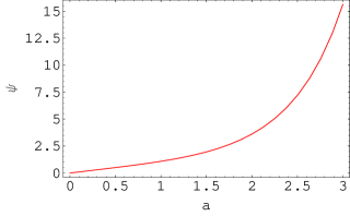
Figure 1: Plot of the $\psi(a)$ wave function that comes about as a solution of Eq. (61), as a function of the scale factor of the universe, in the regime where a is very small and $4k\gamma=1$. Initial conditions used $\psi(a=0)=0,\frac{d}{da}\psi(a=0)=1$.

We conclude, by providing the graph of $\psi(a)$ as a function of the scale factor for $4k\gamma=1$. This shows, that the universe emerges out of nothing (zero scale factor) from zero probability density to a nonzero scale factors with $|\psi(a)|^{2}>0$. We note, that in general satisfying the Dewitt boundary condition is really hard since in most cases it leads to trivial models (i.e. vanishing wave function for any scale factor). However, in our analysis no such problem is encountered.

IV Quantum Cosmology for Non-minimal Tachyon-Gravity couplings

The DBI action associated to the moduli field $\phi$ is known to be similar to the one of the tachyon. This is easily seen for a tachyon potential of the form $\sim{T^{-4}}$ followed by a proper redifintion of fields Silverstein:2003hf . Even though the model we described in the previous section has no relation to the tachyon other than the fact that they both share similar actions (since Silverstein-Tong model is shown Silverstein:2003hf to be free of tachyonic instabilities) it would be interesting to see whether one can uncover other similarities in their dynamics when viewed from a quantum cosmology perspective. We expect for instance, that for a typical tachyonic potential (which is widely used in tachyon cosmology) of the following form $V(T)\sim{e^{-T^{2}}}$, the cosmological equation of motions of the tachyon will differ in general from the corresponding FRW equations of the moduli $\phi$ due to the non trivial potential. Things can get more complicated if higher order gravity tachyonic couplings are included. Thus, in this section our primary concern is to employ the minisuperspace formalism for the case of the tachyon being non-minimally coupled to gravity. While such couplings have been well explored Sen:1999md in terms of string theory, there hasn’t been any specific quantum cosmological application so far. We also note, that in Piao:2002nh ,Chingangbam:2004ng the authors investigated the importance of this type of coupling inside the scope of inflationary cosmology. We basically follow the notation of Chingangbam:2004ng through the rest of the section.

Let us begin by considering the following action describing the non-minimal tachyon-gravity coupling

$$S=\int d^{4}x\sqrt{-g}(\frac{M^{2}_{P}}{2}Rf(T)-AV(T)\sqrt{1+Bg^{\mu\nu}\partial_{\mu}T\partial{\nu}T})$$ (65)

where $A=\sqrt{2}/(2\pi)^{3}g{\alpha^{\prime}}^{2}$, $B=8ln2{\alpha^{\prime}}$, $M^{2}_{P}=u/g^{2}{\alpha^{\prime}}$ and $u=2V_{6}/(2\pi)^{7}{\alpha^{\prime}}^{3}$.

With $V_{6}$ we denote the volume of the compactified manifold while u is a dimensional constant. The tachyon potential $V(T)$ can be taken to have the following asymptotic behavior: $V(T)\sim{e^{-T^{2}}}$ for $T\rightarrow{0}$ while for $T\rightarrow{\infty}$ the potential reads $V(T)\sim{e^{-T}}$. These are the conventional forms used in tachyon cosmology. While in our system B is a constant, one can consider it to be a function of the tachyon field as well Choudhury:2002xu . The action we investigate is not written in the Einstein frame. Therefore, it is wise to perform the following tachyon dependent conformal transformation $g_{\mu\nu}\rightarrow{f(T)g_{\mu\nu}}$ that transforms Eq. (65) into

$$S=\int d^{x}\sqrt{g}(\frac{M^{2}_{P}}{2}(R-\frac{3}{2}\frac{f^{\prime 2}}{f^{2}}g^{\mu\nu}\partial_{\mu}T\partial_{\nu}T)-A\tilde{V(T)}\sqrt{1+Bf(T)g^{\mu\nu}\partial_{\mu}T\partial{\nu}T})$$ (66)

where the rescaled tachyon potential reads $\tilde{V(T)}=V(T)/f(T)^{2}$. For a closed FRW metric the Lagrangian is as follows

$$L=\frac{6\pi^{2}}{M^{2}_{P}}((a(1-\dot{a}^{2})+\frac{1}{4}\frac{f^{\prime 2}}{f^{2}}a^{3}\dot{T}^{2})M^{4}_{P})-\frac{M^{2}_{p}}{6}A\tilde{V(T)}a^{3}\sqrt{1-Bf\dot{T}^{2}})$$ (67)

For the case where the tachyon velocity is much smaller than its upper limit, namely $1>>Bf\dot{T}^{2}$, then by expanding the radical up to first order in $\dot{T}^{2}$ we end up with

$$L=\frac{6\pi^{2}}{M^{2}_{P}}(a(1-\dot{a}^{2})M^{4}_{P}-\frac{M^{2}_{P}}{6}A\tilde{V}a^{3}+(\frac{1}{4}M^{2}_{P}\frac{f^{\prime 2}}{f^{2}}+\frac{M^{2}_{P}}{12}AB\tilde{V}f)a^{3}\dot{T}^{2})$$ (68)

Next, we repeat the same step by step procedure implemented in the former section in constructing the Hamiltonian of WDW equation corresponding to Eq. (68). The associated canonical momenta are of the form

$$P_{a}=-12\pi^{2}M^{2}_{P}a\dot{a}$$ (69)

$$P_{T}=\frac{12\pi^{2}}{M^{2}_{P}}(\frac{1}{4}M^{4}_{P}\frac{f^{\prime 2}}{f^{2}}+\frac{M^{2}_{P}}{12}AB\tilde{V(T)}f)a^{3}\dot{T}$$ (70)

Thus the Hamiltonian defined as $H=P_{a}\dot{a}+P_{T}\dot{T}-L$ reads

$$H=M^{-4}_{P}(-\frac{M^{2}_{P}}{24\pi^{2}}\frac{1}{a}P^{2}_{a}+\frac{M^{2}_{P}}{24\pi^{2}}\frac{1}{a^{3}}\frac{P^{2}_{T}}{(\frac{1}{4}(\frac{f^{\prime}}{f})^{2}+\frac{1}{12M^{2}_{P}}AB\tilde{V}f)}+6\pi^{2}M^{6}_{P}(-a+\frac{A\tilde{V}}{6M^{2}_{P}}a^{3}))$$ (71)

Proceeding with the canonical quantization of the Hamiltonian at hand and by implementing the ansatz $\Psi(a,T)=\psi(a)\psi(T)$ for the wave function, we find

$$\frac{M^{2}_{P}}{24\pi^{2}}\frac{1}{a\psi(a)}\frac{\partial^{2}\psi(a)}{\partial{a}^{2}}+\frac{M^{2}_{P}}{24\pi^{2}}\frac{1}{a^{2}\psi(a)}\frac{\partial\psi(a)}{\partial{a}}-\frac{M^{2}_{P}}{24\pi^{2}}\frac{1}{a^{3}(\frac{1}{4}(\frac{f^{\prime}}{f})^{2}+\frac{AB\tilde{V}f}{M^{2}_{P}})}\frac{1}{\psi(T)}\frac{\partial^{2}\psi(T)}{\partial{T^{2}}}$$

$$+6\pi^{2}M^{6}_{P}(-a+\frac{A\tilde{V}a^{3}}{6M^{2}_{P}})=0$$ (72)

One of the reasons Eq. (72) is a bit cumbersome, is that the non-minimal coupling gives additional contributions to the kinetic term of the rolling tachyon. Thus, it is quite reasonable to expect a lack of integrability in the equation. As we proceed we will mainly focus on two particular interesting cases. For the first one, our motivation is to obtain cosmological wave functions for both gravity and the tachyon for $\tilde{V}$ and $f$ that satisfy the slow roll condition for inflation to occur Chingangbam:2004ng (even though fitting with the observational data might be difficult). For the second one, we attempt through a particular choice of coupling to render WDW equation integrable and consequently obtain the corresponding wave functions.

Working in the regime where $a>>\frac{A\tilde{V}a^{3}}{6M^{2}_{P}}$ the resulting equations are

$$\frac{M^{2}_{P}}{24\psi^{2}}\frac{1}{(\frac{1}{4}(\frac{f^{\prime}}{f})^{2}+\frac{AB\tilde{V}}{12M^{2}_{P}})}\frac{1}{\psi(T)}\frac{\partial^{2}\psi(T)}{\partial{T^{2}}}=k$$ (73)

$$\frac{M^{2}_{P}}{24\pi^{2}}\frac{a^{2}}{\psi(a)}\frac{\partial^{2}\psi(a)}{\partial{a}^{2}}+\frac{M^{2}_{P}}{24\pi^{2}}\frac{a}{\psi(a)}\frac{\partial\psi(a)}{\partial{a}}-6\pi^{2}M^{6}_{P}a^{4}-k=0$$ (74)

Then by choosing

$$\tilde{V(T)}=1-\frac{1}{4}{T^{4}}+...$$ (75)

$$f(T)=1-\frac{1}{2}T^{2}+\frac{1}{4}T^{4}$$ (76)

together with the condition $AB=6M^{2}_{P}$ Chingangbam:2004ng while keeping terms to the lowest order in T, one gets

$$\psi(T)=c_{1}e^{-\sqrt{2\delta_{2}}T}+c_{2}e^{\sqrt{2\delta_{2}}T}$$ (77)

$$\psi(a)=Z_{\frac{\sqrt{\delta_{2}}}{2}}(\frac{\sqrt{\delta_{1}}}{2}a^{2})$$ (78)

where, $\delta_{1}=144\pi^{4}k$, $\delta_{2}=12\pi^{2}k/M^{2}_{P}$, and k is an integration constant which is taken to be positive. It should be kept in mind, that this solution is valid only close to the top of the tachyon potential ($V\sim{e^{-T^{2}}}$), where inflation can take place. The form of the tachyon wave function is surprisingly simple despite the presence of non-minimal coupling. One can also prove, that the presence of the exponentially increasing term in the $\psi(T)$ is not a problem since the $\psi(T)$ can be shown to be square integrable for small values of the tachyon and with a particular choice of the constants involved.

There is a striking similarity between Eq. (51,52) and Eq. (77,78). Apart from trivial differences in the constants involved, they all appear to be essentially identical. This is quite surprising considering the inclusion of nontrivial couplings in the WDW Hamiltonian. Thus, when the tachyon is very close to the top of the potential the minisuperspace description of the tachyon in a closed four dimensional universe is the same as Silverstein-Tong’s model (for a brane of $S^{3}$ spatially topology). Also, this particular correspondence holds for $k<0$ as one can very easily show. As we shall show later on, this is no longer true when the tachyon starts rolling away from the top i.e. $V(T)\sim{e^{-T/2}}$ for certain types of non minimal gravity tachyon couplings.

In both regimes of small and big values for T, one can find non-minimal couplings that render WDW equation completely integrable. This is easy to see by inspection of Eq. (72). Thus, by demanding that $\tilde{V(T)}=\tilde{V_{0}}=const$, when $V(T)=e^{-T}$ and the size of the universe is small we obtain

$$\psi(T)=Z_{4\sqrt{\lambda_{1}}}(4\sqrt{\lambda_{2}}e^{-T/4})$$ (79)

$$\psi(a)=Z_{\frac{\sqrt{\xi_{2}}}{2}}(\frac{\sqrt{\xi_{1}}}{2}a^{2})$$ (80)

where $\lambda_{1}=3\pi^{2}k/2M^{2}_{P}$, $\lambda_{2}=2\pi^{2}kABV_{0}$ and $\xi_{1}=144\pi^{4}M_{P}$, $\xi_{2}=24\pi^{2}k/M^{2}_{P}$. Both formulae are obtained for $f(T)=e^{-T/2}/\sqrt{\tilde{V_{0}}}$ and for positive integration constant k.

For the case where $V(T)=e^{-T^{2}}$, the appropriate conformal coupling that maintains integrability is $f(T)=e^{-T^{2}/2}/\sqrt{\tilde{V_{0}}}$. As a result, the WDW equation for the tachyon reads

$$\frac{\partial^{2}{\psi(T)}}{\partial{T^{2}}}=(\frac{1}{4}\eta_{1}T^{2}+\eta_{1}\eta_{2}e^{-T^{2}/2})\psi(T)$$ (81)

where $\eta_{1}=24\pi^{2}k/M^{2}_{P}$, $\eta_{2}=AB\tilde{V_{0}}/12M^{2}_{P}$, and $k>0$.

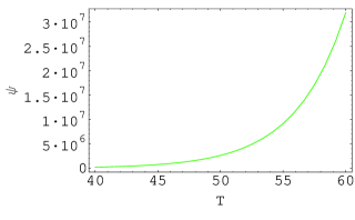
Figure 2: Tachyonic wave function Eq. (79) plotted for when $24\pi^{2}k=M^{2}_{P}$ and $AB\tilde{V_{0}}=12M^{2}_{P}$.

We solve Eq. (81) numerically and show, that even in the case where the tachyon is close to the top of the potential $V(T)=e^{-T^{2}}$ its wave function is increasing almost linearly for small T. Similarly, when the tachyon is away from the top i.e. $V=e^{-T}$ its wave function increases quite rapidly as a function of T as $T\rightarrow{\infty}$. The fact that the wave function is not square integrable, prevents us from interpreting our results in terms of probability densities. However, in theories with tachyons, we expect that as the tachyon rolls it has to reach infinity namely $T\rightarrow{\infty}$, as the condensation takes place. There is no other option for it but to increase its magnitude. Therefore, we expect the “probability density” to find the tachyon in higher expectation values has to increase constantly and maybe that is the reason for unbounded solutions to the WDW Equation.

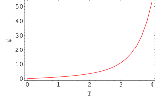
Figure 3: Plot of the tachyon wave function $\psi(T)$ that solves Eq. (81), when $24\pi^{2}k=M^{2}_{P}$ and $AB\tilde{V_{0}}=12M^{2}_{P}$.

V Conclusions

In this paper we present several quantum cosmology aspects of gravitational theories tied to the Dirac-Born-Infeld Lagrangian. Based on $AdS/CFT$ duality, in the strong coupling limit of $N=4$ super Yang Mills theory, the dynamics of the moduli field $\phi$ can be described in terms of the DBI action for a probe D$3$-brane moving in AdS spacetime. Then, we seek cosmological solutions for a universe with $S^{3}$ spatial topology described by the DBI action. We were able to find the asymptotic expressions for the scale factor and the scalar field for a given external potential coupled to gravity. A formal expression for the creation of this particular universe out of “nothing” to a finite small scale factor is recovered in terms of Linde’s prescription.

The above system was further analyzed in terms of the minisuperspace formalism and WDW equation. A variety of solutions was presented for the scale factor and the moduli wave function, both being qualitatively different. At a certain limit, it is shown, that the wave function of the moduli (which become first order differential equation in T) is similar to the one of the tachyon presented in previous works resulting in a time dependent version of the WDW after a proper redefinition of variables. In the later part of this article, there was a discussion regarding the effects of a non-minimal gravity coupling with the tachyon field. In particular, we showed that one can introduce phenomenologically interesting couplings for which the tachyon have similar minisuperspace description with the moduli of D-brane inspired models Silverstein:2003hf . Thus, our analysis clearly indicates the importance of non minimal gravity-tachyon couplings at least within the framework of quantum cosmology. It was also shown, that even for such highly coupled systems, a particular choice of conformal coupling can make the WDW equation of the tachyon to decouple from gravity when the size of the universe is quite small.

One of the possible extensions of the current work would be to implement our minisuperspace description to other possible ambient topologies as was done in Linde:2004nz (yielding regular solutions for zero scalar factors) and generalized in McInnes:2005su for a toroidal universe in terms of Hartle-Hawking and Firouzjahi-Sarangi-Tye wave function Firouzjahi:2004mx . Moreover, further studies of quantum cosmology on compact, flat tachyonic (unstable) universes might also address the issue of accelerating singular toral universes McInnes:2005sa . Finally, in one of the non-minimal couplings that we implemented to make WDW equation integrable i.e. $f(T)=e^{-T^{2}/2}/\sqrt{\tilde{V_{0}}}$, it would be interesting to search for appropriate values for the constant $\tilde{V_{0}}$ for which inflation could occur. Towards this goal, one may introduce an external tachyon potential in the action and study its effects on the universe, even beyond the minisuperspace formalism.

Acknowledgements

The author would like to thank Ioannis Bakas for his constant support, motivation and for his comments on the manuscript. I also thank Pran Nath, Yogi Srivastava, Toamsz Taylor and Allan Widom for carefully reading and commenting on the paper. Finally, i would like to thank the organizers of “Corfu Summer Institute on EPP 2005” for their hospitality, ample financial support and for the excellent, friendly and stimulating environment which contributed in finalizing this work.

References

- (1) B. S. DeWitt, “Quantum Theory Of Gravity. 1. The Canonical Theory,” Phys. Rev. 160, 1113 (1967).
- (2) T. P. Shestakova and C. Simeone, “The problem of time and gauge invariance in the quantization of cosmological models. I: Canonical quantization methods,” Grav. Cosmol. 10, 161 (2004) [arXiv:gr-qc/0409114].
- (3) A. Sen, “Time and tachyon,” Int. J. Mod. Phys. A 18, 4869 (2003) [arXiv:hep-th/0209122].
- (4) J. D. Brown and K. V. Kuchar, Phys. Rev. D 51, 5600 (1995) [arXiv:gr-qc/9409001].
- (5) J. B. Hartle and S. W. Hawking, “Wave Function Of The Universe,” Phys. Rev. D 28, 2960 (1983).
- (6) A. D. Linde, “Quantum Creation Of The Inflationary Universe,” Lett. Nuovo Cim. 39, 401 (1984).
- (7) A. Vilenkin, “Quantum Creation Of Universes,” Phys. Rev. D 30, 509 (1984). A. Vilenkin, “Boundary Conditions In Quantum Cosmology,” Phys. Rev. D 33, 3560 (1986).
- (8) A. Vilenkin, “The quantum cosmology debate,” arXiv:gr-qc/9812027. A. Vilenkin, “Quantum cosmology and eternal inflation,” arXiv:gr-qc/0204061.
- (9) S. W. Hawking and D. N. Page, “Operator Ordering And The Flatness Of The Universe,” Nucl. Phys. B 264, 185 (1986).
- (10) S. W. Hawking and Z. C. Wu, “Numerical Calculations Of Minisuperspace Cosmological Models,” Phys. Lett. B 151, 15 (1985). I. G. Moss and W. A. Wright, “The Wave Function Of The Inflationary Universe,” Phys. Rev. D 29, 1067 (1984).
- (11) Y. Okada and M. Yoshimura, “Inflation In Quantum Cosmology In Higher Dimensions,” Phys. Rev. D 33, 2164 (1986).
- (12) Z. C. Wu, “Quantum Kaluza-Klein Cosmologies. I,” Phys. Lett. B 146, 307 (1984). X. M. Hu and Z. C. Wu, “Quantum Kaluza-Klein Cosmologies. Ii,” Phys. Lett. B 149, 87 (1984).
- (13) L. Anchordoqui, C. Nunez and K. Olsen, “Quantum cosmology and AdS/CFT,” JHEP 0010, 050 (2000) [arXiv:hep-th/0007064].
- (14) D. Z. Freedman, G. W. Gibbons and M. Schnabl, “Matrix cosmology,” AIP Conf. Proc. 743, 286 (2005) [arXiv:hep-th/0411119].
- (15) M. Visser, “Quantum Wormholes,” Phys. Rev. D 43, 402 (1991).
- (16) O. Bertolami, P. D. Fonseca and P. V. Moniz, “Quantum cosmological multidimensional Einstein Yang-Mills model in a R x S**3 x S**d topology,” Phys. Rev. D 56, 4530 (1997) [arXiv:gr-qc/9607015].
- (17) M. Gasperini, “Low-energy quantum string cosmology,” Int. J. Mod. Phys. A 13, 4779 (1998) [arXiv:hep-th/9706049].
- (18) S. Davis, “Higher-derivative quantum cosmology,” Gen. Rel. Grav. 32, 541 (2000) [arXiv:gr-qc/9911021].
- (19) S. Davis and H. Luckock, “The quantum theory of a quadratic gravity theory derived from the heterotic string effective action,” Gen. Rel. Grav. 34, 1751 (2002) [arXiv:gr-qc/0201002].
- (20) V. A. Rubakov, “Quantum cosmology,” arXiv:gr-qc/9910025.
- (21) D. L. Wiltshire, “An introduction to quantum cosmology,” arXiv:gr-qc/0101003.
- (22) S. Carlip, “Quantum gravity: A progress report,” Rept. Prog. Phys. 64, 885 (2001) [arXiv:gr-qc/0108040].
- (23) B. C. Da Cunha and E. J. Martinec, “Closed string tachyon condensation and worldsheet inflation,” Phys. Rev. D 68, 063502 (2003) [arXiv:hep-th/0303087].
- (24) H. Firouzjahi, S. Sarangi and S. H. H. Tye, “Spontaneous creation of inflationary universes and the cosmic landscape,” JHEP 0409, 060 (2004) [arXiv:hep-th/0406107].
- (25) A. Kobakhidze and L. Mersini-Houghton, “Birth of the universe from the landscape of string theory,” arXiv:hep-th/0410213.
- (26) H. Ooguri, C. Vafa and E. P. Verlinde, “Hartle-Hawking wave-function for flux compactifications,” arXiv:hep-th/0502211. S. Gukov, K. Saraikin and C. Vafa, “A stringy wave function for an S**3 cosmology,” arXiv:hep-th/0505204.
- (27) L. Mersini-Houghton, “Can we predict Lambda for the non-SUSY sector of the landscape?,” Class. Quant. Grav. 22, 3481 (2005) [arXiv:hep-th/0504026].
- (28) S. Sarangi and S. H. Tye, “The boundedness of Euclidean gravity and the wavefunction of the universe,” arXiv:hep-th/0505104.
- (29) B. McInnes, “The most probable size of the universe,” Nucl. Phys. B 730, 50 (2005) [arXiv:hep-th/0509035].
- (30) J. B. Hartle, “Generalizing quantum mechanics for quantum gravity,” arXiv:gr-qc/0510126.
- (31) G. Gabadadze and Y. Shang, “Quantum cosmology of classically constrained gravity,” arXiv:hep-th/0511137.
- (32) A. Sen, “Tachyon condensation on the brane antibrane system,” JHEP 9808, 012 (1998) [arXiv:hep-th/9805170].
- (33) A. Sen, “Rolling tachyon,” JHEP 0204, 048 (2002) [arXiv:hep-th/0203211].
- (34) A. Sen, “Tachyon matter,” JHEP 0207, 065 (2002) [arXiv:hep-th/0203265].
- (35) A. Sen, “Field theory of tachyon matter,” Mod. Phys. Lett. A 17, 1797 (2002) [arXiv:hep-th/0204143].
- (36) M. R. Garousi, “Tachyon couplings on non-BPS D-branes and Dirac-Born-Infeld action,” Nucl. Phys. B 584, 284 (2000) [arXiv:hep-th/0003122].
- (37) E. A. Bergshoeff, M. de Roo, T. C. de Wit, E. Eyras and S. Panda, “T-duality and actions for non-BPS D-branes,” JHEP 0005, 009 (2000) [arXiv:hep-th/0003221].
- (38) J. Kluson, “Proposal for non-BPS D-brane action,” Phys. Rev. D 62, 126003 (2000) [arXiv:hep-th/0004106].
- (39) A. Mazumdar, S. Panda and A. Perez-Lorenzana, “Assisted inflation via tachyon condensation,” Nucl. Phys. B 614, 101 (2001) [arXiv:hep-ph/0107058].
- (40) D. Choudhury, D. Ghoshal, D. P. Jatkar and S. Panda, “On the cosmological relevance of the tachyon,” Phys. Lett. B 544, 231 (2002) [arXiv:hep-th/0204204].
- (41) D. Cremades, F. Quevedo and A. Sinha, “Warped tachyonic inflation in type IIB flux compactifications and the open-string completeness conjecture,” arXiv:hep-th/0505252.
- (42) G. W. Gibbons, “Thoughts on tachyon cosmology,” Class. Quant. Grav. 20, S321 (2003) [arXiv:hep-th/0301117].
- (43) K. L. Panigrahi, “D-brane dynamics in Dp-brane background,” Phys. Lett. B 601, 64 (2004) [arXiv:hep-th/0407134].
- (44) A. Sen, “Tachyon dynamics in open string theory,” Int. J. Mod. Phys. A 20, 5513 (2005) [arXiv:hep-th/0410103].
- (45) A. Ghodsi and A. E. Mosaffa, “D-brane dynamics in RR deformation of NS5-branes background and tachyon cosmology,” Nucl. Phys. B 714, 30 (2005) [arXiv:hep-th/0408015].
- (46) H. Singh, “More on tachyon cosmology in de Sitter gravity,” arXiv:hep-th/0505012.
- (47) H. Yang and B. Zwiebach, “Rolling closed string tachyons and the big crunch,” JHEP 0508, 046 (2005) [arXiv:hep-th/0506076].
- (48) J. M. Maldacena, “The large N limit of superconformal field theories and supergravity,” Adv. Theor. Math. Phys. 2, 231 (1998) [Int. J. Theor. Phys. 38, 1113 (1999)] [arXiv:hep-th/9711200].
- (49) D. Kabat and G. Lifschytz, “Gauge theory origins of supergravity causal structure,” JHEP 9905, 005 (1999) [arXiv:hep-th/9902073].
- (50) E. Silverstein and D. Tong, “Scalar speed limits and cosmology: Acceleration from D-cceleration,” Phys. Rev. D 70, 103505 (2004) [arXiv:hep-th/0310221].
- (51) D. Kutasov, “D-brane dynamics near NS5-branes,” arXiv:hep-th/0405058.
- (52) H. Yavartanoo, “Cosmological solution from D-brane motion in NS5-branes background,” arXiv:hep-th/0407079.
- (53) A. Kehagias and E. Kiritsis, “Mirage cosmology,” JHEP 9911, 022 (1999) [arXiv:hep-th/9910174].
- (54) D. H. Jeong and J. Y. Kim, “Mirage cosmology with an unstable probe D3-brane,” Phys. Rev. D 72, 087503 (2005) [arXiv:hep-th/0502130].
- (55) A. Psinas, “Mirage cosmology of U(1) gauge field on unstable D3 brane universe,” JHEP 0601, 138 (2006) [arXiv:hep-th/0509001].
- (56) H. Q. Lu, Z. G. Huang and W. Fang, “Quantum and classical cosmology with Born-Infeld scalar field,” arXiv:hep-th/0504038.
- (57) H. Garcia-Compean, G. Garcia-Jimenez, O. Obregon and C. Ramirez, “Tachyon driven quantum cosmology in string theory,” Phys. Rev. D 71, 063517 (2005).
- (58) Y. S. Piao, Q. G. Huang, X. m. Zhang and Y. Z. Zhang, “Non-minimally coupled tachyon and inflation,” Phys. Lett. B 570, 1 (2003) [arXiv:hep-ph/0212219].
- (59) P. Chingangbam, S. Panda and A. Deshamukhya, “Non-minimally coupled tachyonic inflation in warped string background,” JHEP 0502, 052 (2005) [arXiv:hep-th/0411210].
- (60) O. Aharony, S. S. Gubser, J. M. Maldacena, H. Ooguri and Y. Oz, “Large N field theories, string theory and gravity,” Phys. Rept. 323, 183 (2000) [arXiv:hep-th/9905111].
- (61) A. A. Tseytlin, “*No-force* condition and BPS combinations of p-branes in 11 and 10 dimensions,” Nucl. Phys. B 487, 141 (1997) [arXiv:hep-th/9609212].
- (62) A. G. Muslimov, “On The Scalar Field Dynamics In A Spatially Flat Friedman Universe,” Class. Quant. Grav. 7, 231 (1990).
- (63) M. Alishahiha, E. Silverstein and D. Tong, “DBI in the sky,” Phys. Rev. D 70, 123505 (2004) [arXiv:hep-th/0404084].
- (64) R. Arnowitt, S. Deser and C. W. Misner, “The Dynamics Of General Relativity,” arXiv:gr-qc/0405109.
- (65) E. W. Kolb and M. Turner,“The Early Universe” Frontiers in physics”; v.69.
- (66) L. S.Gradsbteyn and I. M. Ryzik, “Table of integrals,series and products, 3rd edition, Academic Press,”.
- (67) L. Abramowitz and I. A. Stegun, “Handbook of Mathematical functions with Formulas, Graphs, and Mathematical Tables, Dover Publications, Inc., New York,”.
- (68) A. Sen, “Supersymmetric world-volume action for non-BPS D-branes,” JHEP 9910, 008 (1999) [arXiv:hep-th/9909062]. A. A. Tseytlin, “Sigma model approach to string theory effective actions with tachyons,” J. Math. Phys. 42, 2854 (2001) [arXiv:hep-th/0011033]. G. Arutyunov, S. Frolov, S. Theisen and A. A. Tseytlin, “Tachyon condensation and universality of DBI action,” JHEP 0102, 002 (2001) [arXiv:hep-th/0012080]. S. Corley, D. A. Lowe and S. Ramgoolam, “Einstein-Hilbert action on the brane for the bulk graviton,” JHEP 0107, 030 (2001) [arXiv:hep-th/0106067]. A. Fotopoulos and A. A. Tseytlin, “On gravitational couplings in D-brane action,” JHEP 0212, 001 (2002) [arXiv:hep-th/0211101].
- (69) A. Linde, “Creation of a compact topologically nontrivial inflationary universe,” JCAP 0410, 004 (2004) [arXiv:hep-th/0408164].
- (70) B. McInnes, “Pre-inflationary spacetime in string cosmology,” arXiv:hep-th/0511227.