Revamped Braneworld Gravity

Abstract:

Gravity in five-dimensional braneworld backgrounds often exhibits problematic features, including kinetic ghosts, strong coupling, and the vDVZ discontinuity. These problems are an obstacle to producing and analyzing braneworld models with interesting and potentially observable modifications of 4d gravity. We examine these problems in a general $AdS_{5}/AdS_{4}$ setup with two branes and localized curvature from arbitrary brane kinetic terms. We use the interval approach and an explicit “straight” gauge-fixing. We compute the complete quadratic gauge-fixed effective 4d action, as well as the leading cubic order corrections. We compute the exact Green’s function for gravity as seen on the brane. In the full parameter space, we exhibit the regions which avoid kinetic ghosts and tachyons. We give a general formula for the strong coupling scale, i.e. the energy scale at which the linearized treatment of gravity breaks down, for relevant regions of the parameter space. We show how the vDVZ discontinuity can be naturally but nontrivially avoided by ultralight graviton modes. We present a direct comparison of warping versus localized curvature in terms of their effects on graviton mode couplings. We exhibit the first example of DGP-like crossover behavior in a general warped setup.

1 Introduction

Gravity in five-dimensional braneworld backgrounds exhibits features which, from a 4d point of view, are both novel and surprising. Examples include:

• Kaluza-Klein (KK) graviton modes whose couplings to brane matter are only TeV suppressed [1], and thus potentially detectable as resonances at the LHC [2]–[4].

• Extra 4d scalar modes (radions) whose couplings to brane matter are TeV suppressed but otherwise like those of gravity [5]–[12].

• Continuum KK graviton modes which are potentially detectable at the LHC [13],[14].

• KK graviton modes whose couplings to brane matter are suppressed by warping [15],[16].

• KK graviton modes whose couplings to brane matter are suppressed by localized curvature (i.e. brane kinetic terms for gravity) [17].

• 4d effective theories with no massless graviton [16],[17].

• 4d effective theories with a massless graviton and an additional ultralight KK graviton, whose mass goes to zero in a well-defined parametric limit [18]–[19].

• A crossover scale, such that KK gravitons with mass below this scale have unsuppessed couplings to brane matter, but heavier KK modes have suppressed couplings. This leads to modifications of 4d gravity which appear in the infrared rather than the ultraviolet [17],[20]–[22]. Such “DGP” scenarios could have relevance to cosmology [23]–[25].

What is truely remarkable is that these novel features of gravity do not require the assumption of any new physics beyond a single extra dimension and the existence of co-dimension one branes. The above results are derived in low energy linearized effective descriptions which require no assumptions about quantum gravity, string theory, or the existence of exotic matter.

Before we celebrate too loudly, however, we should confront a number of troubling issues common to most or all braneworld gravity models:

• Are these low energy effective descriptions really just special cases of 5d General Relativity? This is not obvious since most models invoke orbifold backgrounds, and since they also ignore the problem of ultraviolet matching to e.g. the microscopic features of the branes.

• What are the physical degrees of freedom in these various models? This is a difficult question to answer rigorously, since the usual gauge-fixing choices (e.g. harmonic gauge) are not suitable for setups with more than one brane.

• Are these models stable? Models with massless radions are at best marginally stable. Some simple setups [26]–[29] have radions which are kinetic ghosts, i.e. their kinetic terms have the wrong sign. Kinetic ghosts indicate an instability in the model. As we will see in this paper, graviton modes can also be kinetic ghosts, and some kinetic ghosts are also tachyons. Although kinetic ghosts may be useful for some purposes [30]–[33], their presence cannot safely be ignored.

• Under what conditions do ultralight graviton modes mimic 4d gravity, avoiding the famous vDVZ discontinuity [34]?

• At what scale does the low energy linearized approximation break down? Perturbation theory involves more input parameters than just the 5d gravitational coupling $M$; it would not be surprising if in certain limits of these additional parameters the low energy effective theory breaks down at a scale much lower than $M$. Indeed this is precisely what happens in the simplest models containing ultralight graviton modes or crossover behavior, where strong coupling sets in at a scale parametrically much smaller than $M$.

In a recent investigation [35] three of us resolved the first two issues listed above. We recast the standard braneworld models in the “interval picture”, where orbifolding is replaced by intervals with boundaries. We showed that braneworld gravity has a well-defined action principle only if we extend General Relativity to include “brane-boundary equations” which supplement the usual bulk Einstein equations. We also showed how to rigorously extract the physical degrees of freedom, by introducing a class of “straight” gauges suitable for braneworld analysis.

The purpose of this paper is to address the remaining three issues listed above, and thus to revamp the promising field of braneworld gravity. In section 2 we derive the general 4d quadratic effective action for a general setup with two branes, including warping and localized curvature. This action is gauge-fixed to just the physical degrees of freedom, using a straight gauge. In section 3 we use this effective action to demonstrate the presence or absence of kinetic ghosts and/or tachyons according to various choices of the input parameters. This analysis is a generalization and improvement of earlier attempts [36], [37]. We find that both the radion and the graviton zero mode can be kinetic ghosts in certain regions of the parameter space.

In section 4 we address the question of strong coupling. By computing the relevant part of the 4d cubic effective action, we give a general formula to determine the strong coupling scale for the radion. We show that the strong coupling scale becomes small in a DGP-like limit. In section 5 we give an exact expression for the straight gauge graviton Green’s function on the brane. This allows us to show how the vDVZ discontinuity is avoided in warped models with ultralight graviton modes. In a DGP-like limit, our straight gauge graviton Green’s function does not have any diverging tensor structures such as those that appear in DGP; the potential breakdown of linearized gravity in this limit is entirely due to the radion.

Finally, in section 6 we use the exact Green’s function to study the couplings of KK gravitons to brane matter. In the special case of the Karch-Randall setup, we regain the recent results of Kaloper and Sorbo [38]. We focus on models with an infinite extra dimension and no massless graviton. Localized curvature and warping both have the effect of making an ultralight graviton from the first massive KK mode. We compare these two effects in our models, and show that the warping effect is more efficient than localized curvature in creating a simulacrum of 4d gravity.

In section 6 we exhibit explict crossover behavior for models in our general setup. In these models the couplings of the KK graviton modes to brane matter are unsuppressed up to a mass scale $1/r_{c}$, and are highly suppressed for modes heavier than this scale. This behavior is the most interesting phenomenological feature of DGP braneworld gravity; here we can study it in a general warped framework.

2 The 4d quadratic effective action

In [35], a brane world gravity theory with the action

$$S = \int d^{4}x\,\left(\int^{L^{-}}_{0^{+}}dy+\int^{0^{-}}_{-L^{+}}dy\right)\sqrt{-G}\Big{(}2M^{3}R-\Lambda\Big{)}$$ (1)

$$+\sum_{i}\int_{y=y_{i}}d^{4}x\sqrt{-g^{(i)}}(2M_{i}^{2}\tilde{\cal R}^{(i)}-V_{i})+4M^{3}\oint_{\partial\cal M}K\,.$$

was analyzed. This action represents a general warped gravity setup with codimension one branes, written in the interval picture. In (1) $M$ is the 5d Planck scale, $\Lambda=-24M^{3}k^{2}$ is the bulk cosmological constant giving a bulk curvature $k$, the $M_{i}$ are the coefficients of brane-localized curvatures $\tilde{\cal R}^{(i)}$, the $V_{i}$ are brane tensions, and $K$ is the extrinsic curvature of the Gibbons-Hawking boundary term.

Upon linearization, $G_{MN}=G^{\bf 0}_{MN}+h_{MN}$, the $AdS_{5}/AdS_{4}$ background solution is

$$G^{\rm\bf 0}_{MN}=\begin{pmatrix}g^{\rm\bf 0}_{\mu\nu}&0\\ 0&1\end{pmatrix}\,,$$ (2)

where

$$g^{\rm\bf 0}_{\mu\nu}=\frac{a(y)^{2}}{(1-\frac{H^{2}x^{2}}{4})^{2}}\eta_{\mu\nu}\,,$$ (3)

with

$$a(y)=\frac{\cosh k(y-y_{0})}{\cosh ky_{0}}\;,\quad 0<y<L\;,$$ (4)

$\eta_{\mu\nu}={\rm diag}(-1,1,1,1)$ and $x^{2}=\eta_{\mu\nu}x^{\mu}x^{\nu}$. Hereafter, we will omit the superscript ⁰.

It is extremely convenient to trade $M_{i}$ and $V_{i}$ for dimensionless input parameters $v_{i}$ and $w_{i}$ defined by

$$v_{i}=kM_{i}^{2}/M^{3}\;,\qquad w_{i}=V_{i}/2kM^{3}\;.$$ (5)

The brane separation $L$ and the warping parameter $y_{0}$ are then determined from these inputs by the relations

$$T_{i} = \frac{w_{i}}{12}+\frac{v_{i}}{2}(1-T_{i}^{2})\,,$$ (6)

or

$$T_{i}^{\pm}=\frac{1}{v_{i}}\Big{(}-1\pm\sqrt{1+\frac{1}{6}w_{i}v_{i}+v_{i}^{2}}\,\Big{)}\,,$$ (7)

with

$$T_{0}=\tanh ky_{0}\;,\qquad T_{L}=\tanh k(L-y_{0})\;.$$ (8)

The $AdS_{4}$ inverse radius of curvature $H$ is given by

$$H=\frac{k}{{\rm cosh}\,ky_{0}}\;.$$ (9)

Solving $-1<T_{i}^{+}<1$, Figure 1 shows the range of input parameters which gives $AdS_{5}/AdS_{4}$ backgrounds.

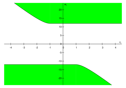
Figure 1: The unshaded area is where $-1<T_{i}^{+}<1$. On the boundary, the curved lines are described by $w_{i}=-6v_{i}-\frac{6}{v_{i}}$, and the straight lines are $w_{i}=\pm 12$.

Using this background solution, we eliminate gauge degrees of freedom and find the following 4d physical degrees of freedom:

1. At the massive level, we have a KK tower of massive spin-2 particles with 5 degrees of freedom each. We can decompose the graviton explicitly into this tower of massive modes:

   $$h_{\mu\nu}=\sum_{q}b^{(q)}_{\mu\nu}=\sum_{q}{\mathcal{Y}}^{(q)}(y)B^{(q)}_{\mu\nu}(x)\,,$$ (10)

   where $q$ labels the mass, $q=m^{2}/H^{2}$, and

   $${\mathcal{Y}}^{(q)}(y) = P_{(-1+\sqrt{9+4q})/2}^{-2}(z)-\frac{a^{(q)}_{0}}{b^{(q)}_{0}}Q_{(-1+\sqrt{9+4q})/2}^{2}(z)$$ (11)

   $$= P_{(-1+\sqrt{9+4q})/2}^{-2}(z)-\frac{a^{(q)}_{L}}{b^{(q)}_{L}}Q_{(-1+\sqrt{9+4q})/2}^{2}(z)\,;$$

   here $z=\tanh k(y-y_{0})$ and the $P$’s and $Q$’s are associated Legendre functions. The mass spectrum of modes is determined by solving the determinant equation,

   $$a_{0}b_{L}-a_{L}b_{0}=0\;,$$ (12)

   with

   $$a_{0} = \{v_{0}q(1-T_{0}^{2})+(3+\sqrt{9+4q})T_{0}\}\,P_{(-1+\sqrt{9+4q})/2}^{-2}(-T_{0})$$

   $$\qquad+(-5+\sqrt{9+4q})\,P_{(-3+\sqrt{9+4q})/2}^{-2}(-T_{0})$$

   $$= \sqrt{1-T_{0}^{2}}\,\{v_{0}q\sqrt{1-T_{0}^{2}}\,P_{(-1+\sqrt{9+4q})/2}^{-2}(-T_{0})-2P_{(-1+\sqrt{9+4q})/2}^{-1}(-T_{0})\}\,,$$

   $$b_{0} = q\sqrt{1-T_{0}^{2}}\,\{v_{0}\sqrt{1-T_{0}^{2}}\,Q_{(-1+\sqrt{9+4q})/2}^{2}(-T_{0})+2Q_{(-1+\sqrt{9+4q})/2}^{1}(-T_{0})\}\,,$$ (13)

   $$a_{L} = \sqrt{1-T_{L}^{2}}\{v_{L}q\sqrt{1-T_{L}^{2}}\,P_{(-1+\sqrt{9+4q})/2}^{-2}(T_{L})+2P_{(-1+\sqrt{9+4q})/2}^{-1}(T_{L})\}\,,$$

   $$b_{L} = q\sqrt{1-T_{L}^{2}}\,\{v_{L}\sqrt{1-T_{L}^{2}}\,Q_{(-1+\sqrt{9+4q})/2}^{2}(T_{L})-2Q_{(-1+\sqrt{9+4q})/2}^{1}(T_{L})\}\,.$$

2. At the massless level, there is a massless spin-2 particle (graviton) $\beta_{\mu\nu}$ with 2 degrees of freedom and a 4d scalar (radion) $\psi(x)$. Thus $h_{\mu\nu}$ is

   $$h_{\mu\nu}=\beta_{\mu\nu}+a^{2}{\mathcal{Y}}_{1}(y)\tilde{\nabla}_{\mu}\tilde{\nabla}_{\nu}\psi+g_{\mu\nu}{\mathcal{Y}}_{2}(y)\psi\,.$$ (14)

   The $y$-dependence of $\beta_{\mu\nu}$ is determined to be

   $$\beta_{\mu\nu}=a^{2}(y)B_{\mu\nu}(x)\,.$$ (15)

   The remaining $y$-dependence is in the ${\mathcal{Y}}_{i}$’s, which are given by

   $${\mathcal{Y}}_{1}(y)=c(1-z)^{2}+dz-{\mathfrak{F}}\,,\quad{\mathcal{Y}}_{2}(y)=-H^{2}c(1-z)^{2}-H^{2}dz+\frac{a^{\prime}}{a}{\mathcal{F}}\,,$$ (16)

   where

   $$c = \frac{k}{H^{2}}\frac{{\mathcal{F}}(L)-{\mathcal{F}}(0)}{\alpha_{0}-\alpha_{L}}\,,$$ (17)

   $$d = \frac{k}{H^{2}}\frac{\alpha_{0}{\mathcal{F}}(L)-\alpha_{L}{\mathcal{F}}(0)}{\alpha_{0}-\alpha_{L}}\,,$$ (18)

   with

   $$\alpha_{i}=\frac{2(1-\theta_{i}T_{i})-\theta_{i}k\lambda_{i}(1-\theta_{i}T_{i})^{2}}{1+k\lambda_{i}T_{i}}\,,$$ (19)

   where we have borrowed a notation from [35]: $\theta_{0}=-1$, $\theta_{L}=+1$. The above formulas show a residual gauge freedom parametrized by a single real function $F(y)$, such that ${\mathcal{F}}^{\prime}(y)=F(y)$ and ${\mathfrak{F}}^{\prime}(y)={\mathcal{F}}/a^{2}(y)$.

Using the background solutions, we can expand the action (1) up to the second order in an arbitrary metric fluctuation $h^{MN}$. The bulk part becomes

$$2\int d^{4}x\int_{0}^{L}dy\sqrt{-g}\Big{(}-8k^{2}+k^{2}h^{2}+\frac{1}{2}R_{MPNQ}h^{MN}h^{PQ}$$

$$\qquad-\frac{1}{4}\nabla_{P}h^{MN}\nabla^{P}h_{MN}+\frac{1}{4}\nabla_{M}h\nabla^{M}h-\frac{1}{2}\nabla_{M}h\nabla_{N}h^{MN}+\frac{1}{2}\nabla_{M}h^{MN}\nabla_{P}h^{P}_{N}$$

$$\qquad+\nabla_{M}(\nabla_{N}h^{MN}-\nabla^{M}h-\frac{3}{2}h^{MN}\nabla^{P}h_{PN}-\frac{1}{2}h^{PN}\nabla_{P}h^{M}_{N}$$

$$\qquad\qquad+h^{MN}\nabla_{N}h+\frac{1}{2}h\nabla_{N}h^{MN}+h^{PN}\nabla^{M}h_{PN}-\frac{1}{2}h\nabla^{M}h)\Big{)}\,,$$ (20)

the brane part is, with 4d total divergence terms dropped,

$$\sum_{i}\int d^{4}x\Big{[}\sqrt{-g}\Big{(}-\frac{12\lambda_{i}H^{2}}{a^{2}}-U_{i}-\Big{(}\frac{3\lambda_{i}H^{2}}{a^{2}}+\frac{U_{i}}{2}\Big{)}\tilde{h}$$

$$\qquad+\lambda_{i}(-\frac{1}{4}\tilde{\nabla}_{\rho}h^{\mu\nu}\tilde{\nabla}^{\rho}h_{\mu\nu}+\frac{1}{4}\tilde{\nabla}_{\mu}\tilde{h}\tilde{\nabla}^{\mu}\tilde{h}-\frac{1}{2}\tilde{\nabla}_{\mu}\tilde{h}\tilde{\nabla}_{\nu}h^{\mu\nu}+\frac{1}{2}\tilde{\nabla}_{\mu}h^{\mu\nu}\tilde{\nabla}_{\rho}h^{\rho}_{\nu})$$

$$\qquad+\Big{(}\frac{2\lambda_{i}H^{2}}{a^{2}}+\frac{U_{i}}{4}\Big{)}h^{\mu\nu}h_{\mu\nu}-\Big{(}\frac{\lambda_{i}H^{2}}{2a^{2}}+\frac{U_{i}}{8}\Big{)}\tilde{h}^{2}\Big{)}\Big{]}_{y=y_{i}}\,,$$ (21)

and the extrinsic curvature part turns into

$$2\int d^{4}x\Big{[}\sqrt{-g}\Big{(}\frac{8a^{\prime}}{a}+\tilde{h}^{\prime}+\frac{4a^{\prime}}{a}\tilde{h}-\frac{4a^{\prime}}{a}h_{44}$$

$$\qquad+\frac{1}{4}\tilde{h}^{2}{}^{\prime}+\frac{a^{\prime}}{a}\tilde{h}^{2}-h^{\mu\nu}h_{\mu\nu}^{\prime}-\frac{2a^{\prime}}{a}\tilde{h}h_{44}-\frac{1}{2}\tilde{h}{}^{\prime}h_{44}+\frac{3a^{\prime}}{a}h_{44}^{2}\Big{)}\Big{]}_{y=0}^{y=L}\,.$$ (22)

A tilde indicates that the corresponding entity is a 4d quantity constructed with $g_{\mu\nu}$. Note that there are 5d-total derivative terms in the bulk part. Due to the finiteness of the 5th dimension, they do not vanish identically but make contribution to the brane-boundary part of the action.

Expanding further the bulk part, with the help of

$$\nabla_{\mu}T^{\nu}=\tilde{\nabla}_{\mu}T^{\nu}+\frac{a^{\prime}}{a}\delta^{\nu}_{\mu}T^{4}\,,\quad\nabla_{\mu}T^{4}=\tilde{\nabla}_{\mu}T^{4}-\frac{a^{\prime}}{a}T_{\mu}\,,$$ (23)

and imposing the partial gauge choice $h_{\mu 4}=0$, (2)+(2) +(2) becomes

$$\frac{S}{2M^{3}} = 2\int d^{4}x\int_{0}^{L}dy\sqrt{-g}\Big{(}-8k^{2}-\frac{1}{2}h^{\mu\nu}\tilde{\nabla}_{\mu}\tilde{\nabla}_{\rho}h^{\rho}_{\nu}-\frac{1}{4}\tilde{h}\tilde{\nabla}^{2}\tilde{h}$$ (24)

$$\quad+\frac{1}{4}h^{\mu\nu}\tilde{\nabla}^{2}h_{\mu\nu}+\frac{1}{2}h^{\mu\nu}\tilde{\nabla}_{\mu}\tilde{\nabla}_{\nu}\tilde{h}-\frac{1}{2}\tilde{h}\tilde{\nabla}^{2}h_{44}+\frac{1}{2}h_{44}\tilde{\nabla}_{\mu}\tilde{\nabla}_{\nu}h^{\mu\nu}$$

$$\quad-\frac{1}{4}h^{\mu\nu}{}^{\prime}h_{\mu\nu}{}^{\prime}+\frac{H^{2}-2a^{\prime}{}^{2}}{2a^{2}}h^{\mu\nu}h_{\mu\nu}+\frac{k^{2}a^{2}+a^{\prime}{}^{2}}{2a^{2}}\tilde{h}^{2}+\frac{\tilde{h}^{\prime}{}^{2}}{4}+\frac{a^{\prime}}{4a}\tilde{h}^{2}{}^{\prime}$$

$$\quad+\frac{a^{\prime}}{a}h_{44}^{2}{}^{\prime}+\frac{k^{2}a^{2}+6a^{\prime}{}^{2}}{a^{2}}h_{44}^{2}-\frac{a^{\prime}}{2a}\tilde{h}h_{44}{}^{\prime}-\frac{2a^{\prime}}{a}\tilde{h}^{\prime}h_{44}+\frac{k^{2}a^{2}-3a^{\prime}{}^{2}}{a^{2}}\tilde{h}h_{44}\Big{)}$$

$$+\sum_{i}\int d^{4}x\Big{[}\sqrt{-g}\Big{(}-\frac{4\lambda_{i}H^{2}}{a^{2}}+\frac{U_{i}}{3}$$

$$\quad+\lambda_{i}(-\frac{1}{2}h^{\mu\nu}\tilde{\nabla}_{\mu}\tilde{\nabla}_{\rho}h^{\rho}_{\nu}-\frac{1}{4}\tilde{h}\tilde{\nabla}^{2}\tilde{h}+\frac{1}{4}h^{\mu\nu}\tilde{\nabla}^{2}h_{\mu\nu}+\frac{1}{2}h^{\mu\nu}\tilde{\nabla}_{\mu}\tilde{\nabla}_{\nu}\tilde{h})$$

$$\quad+\frac{\lambda_{i}H^{2}}{2a^{2}}h^{\mu\nu}h_{\mu\nu}-\frac{U_{i}}{24}\tilde{h}^{2}-2kT_{i}h_{44}^{2}+kT_{i}\tilde{h}h_{44}\Big{)}\Big{]}_{y=y_{i}}\,.$$

Note that all the terms linear in $h$ get cancelled, as they should be.

To get a simpler form, we remove $y$-derivatives on the fields whenever it’s possible. For example,

$$\sqrt{-g}\,\frac{a^{\prime}}{4a}\tilde{h}^{2}{}^{\prime} = \Big{(}\frac{a^{3}a^{\prime}}{4(1-\frac{H^{2}x^{2}}{4})^{4}}\tilde{h}^{2}\Big{)}^{\prime}-\frac{\tilde{h}^{2}}{4(1-\frac{H^{2}x^{2}}{4})^{4}}(3a^{2}{a^{\prime}}^{2}+a^{3}a^{\prime\prime})$$ (25)

$$= \Big{(}\sqrt{-g}\,\frac{a^{\prime}}{4a}\tilde{h}^{2}\Big{)}^{\prime}-\sqrt{-g}\,\frac{3{a^{\prime}}^{2}+k^{2}a^{2}}{4a^{2}}\tilde{h}^{2}\,,$$

where the first term contributes to the brane-boundary part of the action. This way, we eliminate $\tilde{h}^{2}{}^{\prime}$, $h_{44}^{2}{}^{\prime}$ and $\tilde{h}h_{44}^{\prime}$–terms from the bulk part of the action, to get

$$\frac{S}{2M^{3}} = 2\int d^{4}x\int_{0}^{L}dy\sqrt{-g}\Big{(}-8k^{2}+\frac{H^{2}-2a^{\prime}{}^{2}}{2a^{2}}h^{\mu\nu}h_{\mu\nu}+\frac{H^{2}}{4a^{2}}\tilde{h}^{2}$$ (26)

$$\quad-\frac{1}{2}h^{\mu\nu}\tilde{\nabla}_{\mu}\tilde{\nabla}_{\rho}h^{\rho}_{\nu}-\frac{1}{4}\tilde{h}\tilde{\nabla}^{2}\tilde{h}+\frac{1}{4}h^{\mu\nu}\tilde{\nabla}^{2}h_{\mu\nu}+\frac{1}{2}h^{\mu\nu}\tilde{\nabla}_{\mu}\tilde{\nabla}_{\nu}\tilde{h}$$

$$\quad-\frac{1}{4}h^{\mu\nu}{}^{\prime}h_{\mu\nu}{}^{\prime}+\frac{\tilde{h}^{\prime}{}^{2}}{4}-\frac{1}{2}\tilde{h}\tilde{\nabla}^{2}h_{44}+\frac{1}{2}h_{44}\tilde{\nabla}_{\mu}\tilde{\nabla}_{\nu}h^{\mu\nu}$$

$$\quad+\frac{3a^{\prime}{}^{2}}{a^{2}}h_{44}^{2}-\frac{3a^{\prime}}{2a}\tilde{h}^{\prime}h_{44}+\frac{3H^{2}}{2a^{2}}\tilde{h}h_{44}\Big{)}$$

$$+\sum_{i}\int d^{4}x\Big{[}\sqrt{-g}\Big{(}-\frac{4\lambda_{i}H^{2}}{a^{2}}+\frac{U_{i}}{3}+\frac{\lambda_{i}H^{2}}{2a^{2}}h^{\mu\nu}h_{\mu\nu}+\frac{\lambda_{i}H^{2}}{4a^{2}}\tilde{h}^{2}$$

$$\qquad+\lambda_{i}(-\frac{1}{2}h^{\mu\nu}\tilde{\nabla}_{\mu}\tilde{\nabla}_{\rho}h^{\rho}_{\nu}-\frac{1}{4}\tilde{h}\tilde{\nabla}^{2}\tilde{h}$$

$$\qquad\quad\quad+\frac{1}{4}h^{\mu\nu}\tilde{\nabla}^{2}h_{\mu\nu}+\frac{1}{2}h^{\mu\nu}\tilde{\nabla}_{\mu}\tilde{\nabla}_{\nu}\tilde{h})\Big{)}\Big{]}_{y=y_{i}}\,.$$

Plugging (10) and (14), we finally obtain

$$\frac{S}{2M^{3}}=\frac{S}{2M^{3}}\Big{|}_{\Lambda}+\frac{S}{2M^{3}}\Big{|}_{\rm massive}+\frac{S}{2M^{3}}\Big{|}_{\rm massless}\,,$$ (27)

where

$$\frac{S}{2M^{3}}\Big{|}_{\Lambda} = -16k^{2}\int d^{4}x\sqrt{-\hat{g}}\int_{0}^{L}dy\,a^{4}+\sum_{i}\int d^{4}x\sqrt{-\hat{g}}\Big{[}a^{4}\Big{(}-\frac{4\lambda_{i}H^{2}}{a^{2}}+\frac{U_{i}}{3}\Big{)}\Big{]}_{y=y_{i}}$$ (28)

$$= -6H^{2}{\mathcal{C}}_{g}^{(0)}\,,$$

$$\frac{S}{2M^{3}}\Big{|}_{\rm massive}=2\sum_{q>0}\int d^{4}x\int_{0}^{L}dy\sqrt{-g}\Big{(}\frac{1}{4}b^{(q)\mu\nu}\tilde{\nabla}^{2}b^{(q)}_{\mu\nu}-\frac{1}{4}b^{(q)\mu\nu}{}^{\prime}b^{(q)}_{\mu\nu}{}^{\prime}+\frac{H^{2}-2a^{\prime}{}^{2}}{2a^{2}}b^{(q)\mu\nu}b^{(q)}_{\mu\nu}\Big{)}$$

$$\hskip 70.0pt+\sum_{q>0}\sum_{i}\int d^{4}x\Big{[}\sqrt{-g}\Big{(}\frac{\lambda_{i}}{4}b^{(q)\mu\nu}\tilde{\nabla}^{2}b^{(q)}_{\mu\nu}+\frac{\lambda_{i}H^{2}}{2a^{2}}b^{(q)\mu\nu}b^{(q)}_{\mu\nu}\Big{)}\Big{]}_{y=y_{i}}$$

$$=\sum_{q>0}{\mathcal{C}}^{(q)}_{g}\int d^{4}x\sqrt{-\hat{g}}\Big{(}\frac{1}{4}B^{(q)\hat{\mu}\hat{\nu}}\hat{\nabla}^{2}B^{(q)}_{\mu\nu}+\frac{H^{2}}{2}B^{(q)\hat{\mu}\hat{\nu}}B^{(q)}_{\mu\nu}-\frac{m^{(q)}{}^{2}}{4}B^{(q)\hat{\mu}\hat{\nu}}B^{(q)}_{\mu\nu}\Big{)}\,,$$ (29)

and

$$\frac{S}{2M^{3}}\Big{|}_{\rm massless}=2\int d^{4}x\int_{0}^{L}dy\sqrt{-g}\Big{(}\frac{1}{4}\beta^{\mu\nu}\tilde{\nabla}^{2}\beta_{\mu\nu}-\frac{1}{4}\beta^{\mu\nu}{}^{\prime}\beta_{\mu\nu}{}^{\prime}+\frac{H^{2}-2a^{\prime}{}^{2}}{2a^{2}}\beta^{\mu\nu}\beta_{\mu\nu}\Big{)}$$

$$\hskip 70.0pt+\sum_{i}\int d^{4}x\Big{[}\sqrt{-g}\Big{(}\frac{\lambda_{i}}{4}\beta^{\mu\nu}\tilde{\nabla}^{2}\beta_{\mu\nu}+\frac{\lambda_{i}H^{2}}{2a^{2}}\beta^{\mu\nu}\beta_{\mu\nu}\Big{)}\Big{]}_{y=y_{i}}$$

$$\hskip 70.0pt+2\int d^{4}x\int_{0}^{L}dy\sqrt{-g}\Big{(}-\frac{3}{2}{\mathcal{Y}}_{2}^{2}-\frac{3}{4}H^{2}a^{2}{\mathcal{Y}}_{1}^{\prime}{}^{2}-\frac{3}{2}F{\mathcal{Y}}_{2}\Big{)}\psi{\mathcal{D}}_{4}\psi$$

$$\hskip 70.0pt+\sum_{i}\int d^{4}x\Big{[}\sqrt{-g}\Big{(}-\frac{3\lambda_{i}}{2}{\mathcal{Y}}_{2}^{2}\Big{)}\psi{\mathcal{D}}_{4}\psi\Big{]}_{y=y_{i}}$$

$$={\mathcal{C}}^{(0)}_{g}\int d^{4}x\sqrt{-\hat{g}}\,\Big{(}\frac{1}{4}B^{\hat{\mu}\hat{\nu}}\hat{\nabla}^{2}B_{\mu\nu}+\frac{H^{2}}{2}B^{\hat{\mu}\hat{\nu}}B_{\mu\nu}\Big{)}+{\mathcal{C}}_{\psi}\int d^{4}x\sqrt{-\hat{g}}\,\psi\hat{\mathcal{D}}_{4}\psi\,,$$ (30)

with

$${\mathcal{C}}^{(0)}_{g} = \frac{1-T_{0}^{2}}{k}\sum_{i}\Big{(}\tanh^{-1}T_{i}+\frac{T_{i}+k\lambda_{i}}{1-T_{i}^{2}}\Big{)}\,,$$ (31)

$${\mathcal{C}}^{(q)}_{g} = \frac{k}{H^{2}}\Big{(}2\int_{-T_{0}}^{T_{L}}{\mathcal{Y}}^{(q)}{}^{2}dz+\sum_{i}[v_{i}(1-z^{2}){\mathcal{Y}}^{(q)}{}^{2}]_{y=y_{i}}\Big{)}\,,$$ (32)

$$m^{(q)}{}^{2} = H^{2}\frac{\int_{-T_{0}}^{T_{L}}\frac{\{\partial_{z}((1-z^{2}){\mathcal{Y}}^{(q)})\}^{2}}{1-z^{2}}dz}{\int_{-T_{0}}^{T_{L}}{\mathcal{Y}}^{(q)}{}^{2}dz+\sum_{i}\frac{v_{i}}{2}[(1-z^{2}){\mathcal{Y}}^{(q)}{}^{2}]_{y=y_{i}}}\,,$$ (33)

$${\mathcal{C}}_{\psi} = -\int_{0}^{L}dy\,a^{2}\Big{(}3{\mathcal{Y}}_{2}^{2}+\frac{3}{2}H^{2}a^{2}{\mathcal{Y}}_{1}^{\prime}{}^{2}+3F{\mathcal{Y}}_{2}\Big{)}-\sum_{i}\Big{[}\frac{3\lambda_{i}}{2}a^{2}{\mathcal{Y}}_{2}^{2}\Big{]}_{y=y_{i}}\,.$$ (34)

A hatted entity is defined using the metric without a warp factor. If we include a source term in the action, its coupling to a specific graviton mode will show up like

$$S^{(q)} = 2M^{3}{\mathcal{C}}^{(q)}_{g}\int d^{4}x\sqrt{-\hat{g}}\;\frac{1}{4}B^{(q)\hat{\mu}\hat{\nu}}\hat{\nabla}^{2}B^{(q)}_{\mu\nu}+\cdots+\int d^{4}xdy\sqrt{-g}\;h^{(q)}_{\mu\nu}T^{\mu\nu}$$ (35)

$$= \int d^{4}x\sqrt{-\hat{g}}\;\frac{1}{4}\bar{B}^{(q)\hat{\mu}\hat{\nu}}\hat{\nabla}^{2}\bar{B}^{(q)}_{\mu\nu}+\cdots+\int d^{4}xdy\sqrt{-g}\;\frac{{\mathcal{Y}}^{(q)}(y)}{\sqrt{2M^{3}{\mathcal{C}}^{(q)}_{g}}}\bar{B}^{(q)}_{\mu\nu}T^{\mu\nu}\,,$$

and then we can read off the gravitational coupling constant. In particular, on the 0-brane,

$$\frac{1}{M_{4}^{(q)}}=\frac{{\mathcal{Y}}^{(q)}(0)}{\sqrt{2M^{3}{\mathcal{C}}^{(q)}_{g}}}\,.$$ (36)

3 Avoiding ghosts and tachyons

3.1 ghostbusting

It has been known for some time that brane setups of the type that we are considering are sometimes afflicted with unphysical features. Kinetic ghosts, by which we mean wrong-sign kinetic terms for physical modes in the 4d effective action, are indicative of an instability, similar to the case of their cousin the tachyon. Regions of our input parameter space which produce kinetic ghosts are certainly to be avoided if we are interested in static brane configurations. A kinetic ghost radion can occur for setups with e.g., $v_{0}=v_{L}=0$ and $w_{0}+w_{L}<0$. Intuitively we also expect a kinetic ghost graviton to occur in cases where $v_{0}$ and $v_{L}$ become too negative, i.e. we have too much wrong-sign localized curvature. As we will see, the full story is quite complicated.

The boundary between a region of the input parameter space which has a kinetic ghost, and a region which does not, defines a class of models where the coefficient of the kinetic term of a physical mode is vanishing. After a canonical rescaling of the field, this implies strong coupling once we go beyond the linearized theory. Such regions of strong coupling are to be avoided if we want the 4d effective low energy theory to be valid up to energy scales approaching $k$.

In this section we will map out the input parameter space and identify the region which avoids both kinetic ghosts and strong coupling.

We have already noted that the massless mode of the graviton may be a ghost. When we choose $(v_{0},w_{0})$ such that $T_{0}>0$, Figure 2 and 3 show how $\bar{\mathcal{C}}^{(0)}_{g}\equiv k{\mathcal{C}}^{(0)}_{g}/(1-T_{0}^{2})$ varies as a function of $(v_{L},w_{L})$. $\bar{\mathcal{C}}^{(0)}_{g}$ is zero along each line shown in Figure 2 and 3, positive above it and negative below it. As $T_{0}$ approaches $1$ either by $v_{0}\to+\infty$ or by $w_{0}\to+12$, $\bar{\mathcal{C}}^{(0)}_{g}=0$ line moves to the left.

Figure 2: The $\bar{\mathcal{C}}^{(0)}_{g}=0$ on $(v_{L},w_{L})$-plane when $v_{0}=0.3$ and $w_{0}=10,5,-5,-10$ for the lines from left to right respectively.

Figure 3: The $\bar{\mathcal{C}}^{(0)}_{g}=0$ on $(v_{L},w_{L})$-plane when $w_{0}=5$ and $v_{0}=1.5,0.5,-0.5,-1$ for the lines from left to right respectively.

We can play a similar game with the coefficient, ${\mathcal{C}}_{\psi}$, of the radion. Equation (34) holds irrespective of gauge choice of $F(y)$. Then, in a generic case where $\alpha_{0}-\alpha_{L}\neq 0$, for simplicity we can choose

$${\mathcal{F}}(y)=\chi\Big{(}\frac{y}{L}(\alpha_{L}-\alpha_{0})+\alpha_{0}\Big{)}\,,$$ (37)

where $\chi$ is a remaining real gauge parameter that we leave arbitrary as a check of general covariance for physical results. With this choice we get

$$c=-\frac{1}{H^{2}}\,,\;\;d=0\,.$$ (38)

Then, (34) becomes

$${\mathcal{C}}_{\psi} = \frac{3\chi^{2}H^{2}}{k}\sum_{i}\Big{[}-\frac{1}{2}(\theta_{i}+v_{i}z)\alpha_{i}\Big{(}\frac{z}{1-z^{2}}\alpha_{i}+2\frac{1-z}{1+z}\Big{)}+\Big{(}\theta_{i}-\frac{1-z}{2}v_{i}\Big{)}\frac{(1-z)^{2}}{1+z}\Big{]}_{z=\theta_{i}T_{i}}$$ (39)

$$= \frac{3\chi^{2}H^{2}}{2k}\sum_{i}\frac{(-\theta_{i}+T_{i})(2-\theta_{i}v_{i}+v_{i}T_{i})}{1+v_{i}T_{i}}\,.$$

Figures 4 and 5 show that, if we choose $(v_{0},w_{0})$ such that $T_{0}>0$, then $\bar{\mathcal{C}}_{\psi}\equiv 2k{\mathcal{C}}_{\psi}/3\chi^{2}H^{2}$ is positive above each line. Also, the closer $T_{0}$ is to $+1$, the more convex to the left $\bar{\mathcal{C}}_{\psi}=0$ line gets.

Figure 4: The $\bar{\mathcal{C}}_{\psi}=0$ on $(v_{L},w_{L})$-plane when $v_{0}=0.3$ and $w_{0}=10,5,-5,-10$ for the lines from left to right respectively.

Figure 5: The $\bar{\mathcal{C}}_{\psi}=0$ on $(v_{L},w_{L})$-plane when $w_{0}=5$ and $v_{0}=1.5,0.5,-0.5,-1$ for the lines from left to right respectively.

3.2 tachyons

Equation (12) determines the KK mass spectrum of the graviton. For some range of values of the input parameters, it can have a zero at negative $q$, i.e. negative mass-squared. For example, if we choose $v_{0}=5,w_{0}=3,v_{L}=-7,w_{L}=9$, then (12) has a solution $q=-0.94$.

We will refer to such solutions as tachyons. The tachyons with $-9/4<q<0$ obey the Breitenlohner-Freedman bound [39], and as expected we will find (see section 5.1) that the Euclidean Green’s function for such modes has the same exponentially damped asymptotics as for ordinary massive modes. The tachyons with $q<-9/4$ have oscillatory asymptotics, similar to tachyons in flat space. It turns out that some of the tachyonic solutions also have wrong-sign kinetic terms.

We can expose the tachyonic solutions by analyzing the quantity

$${\mathfrak{D}}\equiv\frac{a_{0}b_{L}-b_{0}a_{L}}{q(1-T_{0}^{2})(1-T_{L}^{2})}\,.$$ (40)

Note that ${\mathfrak{D}}$ takes some finite value at $q=0$, proportional to the residue of the pole from the massless graviton mode. Now we can compare the two quantities

$${\mathfrak{D}}|_{q=0}\,,\qquad{\mathfrak{D}}|_{q\to-\infty}\,.$$ (41)

Suppose we find values for the input parameters such that there are no tachyons in the KK graviton spectrum. Then it must be the case that

$${\mathfrak{D}}|_{q=0}\times{\mathfrak{D}}|_{q\to-\infty}>0\;.$$ (42)

As we vary the input parameters, we may cross the hypersurface in the parameter space defined by ${\mathfrak{D}}|_{q=0}\times{\mathfrak{D}}|_{q\to-\infty}=0$. Just across this boundary are models which each contain a single tachyon. To find this boundary between models with no tachyon and models with a single tachyon, we need explicit expressions for ${\mathfrak{D}}|_{q=0}$ and ${\mathfrak{D}}|_{q\to-\infty}$.

${\mathfrak{D}}|_{q=0}$ can be worked out straightforwardly:

$${\mathfrak{D}}|_{q=0}=-2\sum_{i}\Big{(}\frac{1}{2}\log\frac{1+T_{i}}{1-T_{i}}+\frac{T_{i}+v_{i}}{1-T_{i}^{2}}\Big{)}=-2\bar{\mathcal{C}}_{g}^{(0)}\,,$$ (43)

where we used $\tanh^{-1}x=\frac{1}{2}\log\frac{1+x}{1-x}$.

Before trying to evaluate ${\mathfrak{D}}|_{q\to-\infty}$, note that our solutions of the equations of motion should be real. While $P_{(-1+\sqrt{9+4q})/2}^{-2}(z)$ is always real, $Q_{(-1+\sqrt{9+4q})/2}^{2}(z)$ becomes a complex valued function for $q<-9/4$. Thus for $q>-9/4$ we still write (11) in the form

$${\mathcal{Y}}^{(q)}(y)=AP_{(-1+\sqrt{9+4q})/2}^{-2}(z)+BQ_{(-1+\sqrt{9+4q})/2}^{2}(z)\,,$$ (44)

but for $q<-9/4$ we use relation 8.843 of [40] and relations 3.6.1(4)-(5), 3.3.1(7) of [41] to write the real solution

$${\mathcal{Y}}^{(q)}(y)=AP_{ip-1/2}^{-2}(z)+B\frac{\pi}{2\cosh\pi p}(p^{2}+\frac{9}{4})(p^{2}+\frac{1}{4})P_{ip-1/2}^{-2}(-z)\,,$$ (45)

where we have defined $2ip=\sqrt{9+4q}$. The two expressions match at $p=0$, $q=-9/4$.

Plugging (45) into the brane-boundary equations of motion, we obtain $a_{0}$, $b_{0}$, $a_{L}$, $b_{L}$ which are real for any large and negative $q$, i.e., large and positive $p$:

$$a_{0} = \sqrt{1-T_{0}^{2}}\;\Big{\{}-v_{0}(p^{2}+\frac{9}{4})\sqrt{1-T_{0}^{2}}\,P_{ip-1/2}^{-2}(-T_{0})-2P_{ip-1/2}^{-1}(-T_{0})\Big{\}}\,,$$

$$b_{0} = \sqrt{1-T_{0}^{2}}\;\Big{\{}-v_{0}(p^{2}+\frac{9}{4})\sqrt{1-T_{0}^{2}}\,P_{ip-1/2}^{-2}(T_{0})+2P_{ip-1/2}^{-1}(T_{0})\Big{\}}\,,$$

$$a_{L} = \sqrt{1-T_{L}^{2}}\;\Big{\{}-v_{L}(p^{2}+\frac{9}{4})\sqrt{1-T_{L}^{2}}\,P_{ip-1/2}^{-2}(T_{L})+2P_{ip-1/2}^{-1}(T_{L})\Big{\}}\,,$$ (46)

$$b_{L} = \sqrt{1-T_{L}^{2}}\;\Big{\{}-v_{L}(p^{2}+\frac{9}{4})\sqrt{1-T_{L}^{2}}\,P_{ip-1/2}^{-2}(-T_{L})-2P_{ip-1/2}^{-1}(-T_{L})\Big{\}}\,.$$

Using relations 3.2 (14), 3.4 (1), 2.3.2 (17) from [41], we can derive the asymptotic behavior of the conical function $P_{ip-1/2}^{-m}(\cos\theta)$ for large $p$:

$$P_{ip-1/2}^{-m}(\cos\theta)=\frac{1}{\sqrt{2\pi\sin\theta}}\frac{e^{p\theta}}{p^{m}\sqrt{p}}(1+{\mathcal{O}}(p^{-1}))\,,\qquad 0<\theta<\pi\,,$$ (47)

and thus we get

$${\mathfrak{D}}|_{q\to-\infty}\approx-\frac{1}{p^{2}}\frac{v_{0}v_{L}}{2\pi p\sqrt{\sin\theta_{0}\sin\theta_{L}}}\Big{(}e^{p(2\pi-\theta_{0}-\theta_{L})}-e^{p(\theta_{0}+\theta_{L})}\Big{)}\,,$$ (48)

where $\cos\theta_{i}=T_{i}$.

Now we are ready to look at (42), which implies

$${\mathfrak{D}}|_{q=0}>0\quad{\rm and}\quad{\mathfrak{D}}|_{q\to-\infty}>0\,,$$ (49)

or

$${\mathfrak{D}}|_{q=0}<0\quad{\rm and}\quad{\mathfrak{D}}|_{q\to-\infty}<0\,.$$ (50)

Note that the sign of ${\mathfrak{D}}|_{q\to-\infty}$ is the same as the sign of

$$v_{0}v_{L}(\cos^{-1}T_{0}+\cos^{-1}T_{L}-\pi)\,.$$ (51)

Figure 6 shows the tachyon counting for models in the $(v_{L},w_{L})$ plane when $v_{0}>0$. The sign of ${\mathfrak{D}}|_{q=0}$ flips when we cross the line $\bar{\mathcal{C}}_{g}^{(0)}=0$, which is shown as the solid curve. The sign of (51) flips whenever we cross one of the two dashed straight lines. The vertical dashed line is just $v_{L}=0$. The slanted dashed line is

$$w_{L}=-6(1-T_{0}^{2})v_{L}-12T_{0}\;.$$ (52)

Thus the shaded region in Figure 6 gives models which have a single tachyon (or are not $AdS_{5}/AdS_{4}$). The models in the four unshaded regions have an even number of tachyons. Models in the large unshaded region to the right of $v_{L}=0$ are tachyon-free, as expected.

By further numerical analysis, we find that models in the upper two remaining unshaded regions are also tachyon-free, while models in the lower one have two tachyons. Once we also require $\bar{\mathcal{C}}_{g}^{(0)}>0$, only the middle unshaded area remains. This region is rather special. It contains no tachyons and obeys $\bar{\mathcal{C}}_{g}^{(0)}>0$. However in this region one can see numerically that the massive KK graviton modes are kinetic ghosts.

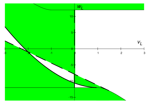
Figure 6: ${\mathfrak{D}}|_{q=0}\times{\mathfrak{D}}|_{q\to-\infty}>0$ on $(v_{L},w_{L})$-plane when $v_{0}=2$ and $w_{0}=1$. The solid curve is where ${\mathfrak{D}}|_{q=0}=0$ and dashed straight lines are ${\mathfrak{D}}|_{q\to-\infty}=0$.

Combining all of the above results with the additional requirement that $\bar{\mathcal{C}}_{\psi}>0$, i.e. no ghost radion, we get figures like Figure 7 for $(v_{0},w_{0})$ chosen such that $T_{0}>0$. Models which are ghost-free and tachyon-free correspond to the unshaded region in the $(v_{L},w_{L})$ plane.

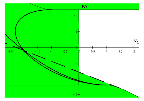
Figure 7: Allowed region (unshaded) on $(v_{L},w_{L})$-plane with $v_{0}=2$ and $w_{0}=1$.

For $v_{0}<0$, a similar analysis finds no region which is free of tachyons and ghosts.

These results fit qualitatively with our physical intuition. Models with negative $M_{i}$ are excluded. Models with too much negative tension branes are also excluded.

A special case is that of an infinite extra dimension. In our general framework we make models of this type by sending $L\to\infty$. We do this by fixing $w_{L}=+12$ and (for simplicity) $v_{L}=0$. In this limit the graviton zero mode is not normalizable and drops out of the theory, so there is no ${\mathcal{C}}_{g}^{(0)}$ to consider. As for ${\mathcal{C}}_{\psi}$, since $T_{L}=+1$, (39) becomes

$${\mathcal{C}}_{\psi}=\frac{3\chi^{2}H^{2}}{2k}\frac{(1+T_{0})(2+v_{0}+v_{0}T_{0})}{1+v_{0}T_{0}}\,,$$ (53)

which is positive for any $v_{0}$ and $w_{0}<12$. Our tachyon analysis reduces to examining $a_{0}|_{q=0}$ and $a_{0}|_{q\to-\infty}$. Since

$$a_{0}|_{q=0}=-(1-T_{0}^{2})<0\,,$$

and

$$a_{0}|_{q\to-\infty}\approx-v_{0}\frac{1-T_{0}^{2}}{\sqrt{2\pi\sin\theta_{0}}}\frac{e^{p(\pi-\theta_{0})}}{\sqrt{p}}\,,$$ (54)

only $v_{0}>0$ is allowed. So in this class of models the allowed region is $v_{0}>0$ and $w_{0}<12$.

4 Strong coupling

For generic choices of the four input parameters $v_{0}$, $w_{0}$, $v_{L}$ and $w_{L}$ we will not have a strong coupling problem, as long as we choose parameters away from the borderline between ghost and non-ghost regions, and away from limits where $H\to 0$.

To determine the strong coupling scale, we need to calculate the cubic action for the radion. See Appendix A for the details of the calculation. The general cubic expansion of the radion part of (1) is

$$\frac{S}{2M^{3}}\Big{|}_{\psi^{3}} = \int d^{4}x\sqrt{-g}\Big{(}{\mathcal{C}}^{(3)}_{1}\hat{\nabla}^{2}\psi\{(\hat{\nabla}^{2}\psi)^{2}-\hat{\nabla}_{\mu}\hat{\nabla}_{\nu}\psi\hat{\nabla}^{\mu}\hat{\nabla}^{\nu}\psi\}$$ (55)

$$\quad+{\mathcal{C}}^{(3)}_{2}\psi\{(\hat{\nabla}^{2}\psi)^{2}-\hat{\nabla}_{\mu}\hat{\nabla}_{\nu}\psi\hat{\nabla}^{\mu}\hat{\nabla}^{\nu}\psi\}+{\mathcal{C}}^{(3)}_{3}\psi^{2}\hat{\nabla}^{2}\psi+{\mathcal{C}}^{(3)}_{4}\psi^{3}\Big{)}\,.$$

When it comes to the strong coupling, ${\mathcal{C}}^{(3)}_{1}$ would be expected to give the most stringent limit. However with $F(y)$ determined by (37), direct calculation shows that

$${\mathcal{C}}^{(3)}_{1} = \sum_{i}\Big{[}\Big{(}\frac{\theta_{i}+v_{i}z}{2(1-z)}{\mathcal{F}}(y)-\chi(\theta_{i}-\frac{1-z}{2}v_{i})\Big{)}$$ (56)

$$\qquad\Big{(}\frac{H^{2}}{4k^{2}}\frac{{\mathfrak{F}}(y)^{2}}{1+z}+\frac{\chi}{2k}\frac{(1-z)^{2}}{1+z}{\mathfrak{F}}(y)+\frac{\chi^{2}}{4H^{2}}\frac{(1-z)^{4}}{1+z}\Big{)}\Big{]}_{y=y_{i}}$$

$$= 0\,,$$

The next candidate, ${\mathcal{C}}^{(3)}_{2}$, turns out to be

$${\mathcal{C}}^{(3)}_{2} = \sum_{i}\theta_{i}\Big{[}-\frac{{\mathcal{F}}(y)^{3}}{12}+\frac{\chi H^{2}}{k^{2}}\frac{F{\mathfrak{F}}(y)}{1+z}\Big{]}_{y=y_{i}}+\frac{2\chi H^{2}}{k}\int_{0}^{L}\frac{F{\mathfrak{F}}(y)}{1+z}dy$$ (57)

$$= \chi^{3}\frac{\alpha_{0}-\alpha_{L}}{12}\Big{\{}\alpha_{0}^{2}+\alpha_{0}\alpha_{L}+\alpha_{L}^{2}+\frac{-12\alpha_{L}T_{0}^{-1}-12\alpha_{0}T_{L}^{-1}+6(\alpha_{0}-\alpha_{L})\log 4}{T_{0}^{-1}+T_{L}^{-1}}$$

$$\qquad+\frac{6(\alpha_{0}-\alpha_{L})}{(T_{0}^{-1}+T_{L}^{-1})^{2}}\Big{(}{\rm Li}_{2}(-\frac{1+T_{0}}{1-T_{0}})-{\rm Li}_{2}(-\frac{1-T_{L}}{1+T_{L}})\Big{)}\Big{\}}\,,$$

where $T_{i}^{-1}=\tanh^{-1}T_{i}$ and ${\rm Li}_{n}$ is a polylogarithm function. This does not vanish. Then from the full radion action

$$S\,|_{\psi} = 2M^{3}{\mathcal{C}}_{\psi}\int d^{4}x\sqrt{-\hat{g}}\,\psi\hat{\nabla}^{2}\psi$$ (58)

$$+2M^{3}{\mathcal{C}}^{(3)}_{2}\int d^{4}x\sqrt{-\hat{g}}\,\psi\{(\hat{\nabla}^{2}\psi)^{2}-\hat{\nabla}_{\mu}\hat{\nabla}_{\nu}\psi\hat{\nabla}^{\mu}\hat{\nabla}^{\nu}\psi\}+\cdots$$

$$= \int d^{4}x\sqrt{-\hat{g}}\,\bar{\psi}\hat{\nabla}^{2}\bar{\psi}$$

$$+\frac{2M^{3}{\mathcal{C}}^{(3)}_{2}}{(2M^{3}{\mathcal{C}}_{\psi})^{3/2}}\int d^{4}x\sqrt{-\hat{g}}\,\bar{\psi}\{(\hat{\nabla}^{2}\bar{\psi})^{2}-\hat{\nabla}_{\mu}\hat{\nabla}_{\nu}\bar{\psi}\hat{\nabla}^{\mu}\hat{\nabla}^{\nu}\bar{\psi}\}+\cdots\,,$$

we can determine the strong coupling scale:

$$\Lambda_{\rm sc}=(2M^{3})^{1/6}\frac{{\mathcal{C}}_{\psi}^{1/2}}{{\mathcal{C}}^{(3)}_{2}{}^{1/3}}\,.$$ (59)

As an example, let’s consider a DGP-like limit ($v_{L}=0$, $w_{L}=+12$, $v_{0}$ is large). Then (59) becomes

$$\Lambda_{\rm sc}\sim\frac{M^{2}}{M_{0}}\sqrt{12-w_{0}}\,,$$ (60)

where our parameter $M_{0}$ is equivalent to the parameter $M_{P}$ in DGP. This agrees well with [42].

In our general framework we can understand the robustness of the strong coupling problem. As long as we restrict ourselves to models in the ghost+tachyon free region of the parameter space, the coefficient $\bar{\mathcal{C}}_{g}^{(0)}$ of the graviton kinetic term never vanishes, as can be seen from (31). From (59) we can see that the radion becomes strongly coupled in any limit where $H\to 0$. This includes the DGP-like limit just mentioned, as well as the “bigravity” limit $T_{0}\to+1$. Unfortunately these are precisely the limits in which we find ultralight graviton modes.

5 Green’s function analysis

In [35], the set of coupled equations of motion of the graviton and the radion was obtained in a straight gauge. Once we eliminate the radion, we get four independent equations involving the graviton only. These are of the form:

$${\mathcal{D}}^{(\rm i)}_{\mu\nu\rho\sigma}h^{\rho\sigma}=0\,,$$ (61)

$${\mathcal{D}}^{(\rm ii)}_{\mu\nu}h^{\mu\nu}=0\,,$$ (62)

$$[{\mathcal{D}}^{(\rm bdy)}_{\mu\nu\rho\sigma}h^{\rho\sigma}]_{y=y_{i}}=0\,,$$ (63)

where the full expressions are given in (B)-(102). These imply the following Green’s function equations in the straight gauge:

$${\mathcal{D}}^{(\rm i)}_{\mu\nu\rho\sigma}G^{\rho\sigma}_{;\mu^{\prime}\nu^{\prime}}=\frac{1}{M^{3}}O_{\mu\nu;\mu^{\prime}\nu^{\prime}}(x,x^{\prime})\frac{\delta^{(4)}(x-x^{\prime})\delta(y-y^{\prime})}{\sqrt{-g}}\,,$$ (66)

$${\mathcal{D}}^{(\rm ii)}_{\mu\nu}G^{\mu\nu}_{;\mu^{\prime}\nu^{\prime}}=0\,,$$

$$[{\mathcal{D}}^{(\rm bdy)}_{\mu\nu\rho\sigma}G^{\rho\sigma}_{;\mu^{\prime}\nu^{\prime}}]_{y=y_{i}}=0\,,$$

where the $AdS_{4}$ bitensor $O_{\mu\nu;\mu^{\prime}\nu^{\prime}}(x,x^{\prime})$ is given below. Then, for any given source, we get the linearized solution for the graviton from

$$h_{\mu\nu}(x,y)=\int d^{4}x^{\prime}dy\sqrt{-g}\,G_{\mu\nu;\mu^{\prime}\nu^{\prime}}(x,y;x^{\prime},y^{\prime})T^{\mu^{\prime}\nu^{\prime}}(x^{\prime},y^{\prime})\,.$$ (67)

In Appendix B, the Euclidean versions of (66)-(66) are explicitly solved to obtain the Euclidean Green’s function. After dropping 4d total derivatives which will vanish when contracted with a conserved stress tensor, we can write the following expression for the Euclidean Green’s function on the 0-brane:

$$G_{\mu\nu\,;\,\mu^{\prime}\nu^{\prime}}(x,x^{\prime},y=y^{\prime}=0)=\sum_{j}G_{1}(u;p_{j})\bigg{\{}\,T^{(3)}_{\mu\nu\,;\,\mu^{\prime}\nu^{\prime}}$$

$$\hskip 45.0pt-\frac{2}{3}\frac{H^{4}}{p_{j}^{2}-\frac{1}{4}}T^{(1)}_{\mu\nu\,;\,\mu^{\prime}\nu^{\prime}}\Big{(}p_{j}^{2}-\frac{9}{4}+3(1+u)^{2}+\frac{3(1+u)}{\frac{d}{du}{\rm ln}\,Q_{p_{j}-\frac{1}{2}}(1+u)}\Big{)}\bigg{\}}\,,$$ (68)

where the sum is over the residues of poles from the individual KK graviton modes. The masses $m_{j}$ of these modes are determined by the solutions of (12), and are expressed in terms of the parameter $p_{j}$:

$$m_{j}^{2}=H^{2}(p_{j}^{2}-\frac{9}{4})\;.$$ (69)

The variable $u$ is related to the geodesic distance $\mu$ between the points $x$ and $x^{\prime}$ in $AdS_{4}$: $u=\cosh H\mu-1$. The function $G_{1}(u;p_{j})$ is given by

$$G_{1}(u;p_{j})=-\frac{1}{4\pi^{2}H^{2}M_{4}^{(j)}{}^{2}}\frac{d}{du}Q_{p_{j}-1/2}(1+u)\;,$$ (70)

where $Q_{p_{j}-1/2}$ is a Legendre function. The $AdS_{4}$ tensor structure of the Green’s function (5) is contained in the bitensors $T^{(1)}$ and $T^{(3)}$, which are part of the complete bitensor basis given in (106):

$$T^{(1)}_{\mu\nu\,;\,\mu^{\prime}\nu^{\prime}} = g_{\mu\nu}g_{\mu^{\prime}\nu^{\prime}}\;,$$

$$T^{(3)}_{\mu\nu\,;\,\mu^{\prime}\nu^{\prime}} = \partial_{\mu}\partial_{\mu^{\prime}}u\partial_{\nu}\partial_{\nu^{\prime}}u+\partial_{\mu}\partial_{\nu^{\prime}}u\partial_{\nu}\partial_{\mu^{\prime}}u\;.$$ (71)

The bitensor on the right hand side of (66) is given by:

$$O_{\mu\nu;\mu^{\prime}\nu^{\prime}}(x,x^{\prime})=\frac{1}{2}(g_{\mu\mu^{\prime}}g_{\nu\nu^{\prime}}+g_{\mu\nu^{\prime}}g_{\nu\mu^{\prime}})\;,$$ (72)

where we have defined bivectors:

$$g_{\mu\mu^{\prime}}(x,x^{\prime})=\partial_{\mu}\partial_{\mu^{\prime}}u-\frac{\partial_{\mu}u\partial_{\mu^{\prime}}u}{2+u}\;.$$ (73)

The bitensor $O_{\mu\nu;\mu^{\prime}\nu^{\prime}}(x,x^{\prime})$ is determined by requiring that it has the property:

$$O_{\mu\nu;\mu^{\prime}\nu^{\prime}}(x,x^{\prime}=x)\,T^{\mu^{\prime}\nu^{\prime}}(x)=T_{\mu\nu}(x)\;,$$ (74)

which can be checked easily using (72), (73).

Apart from the $j$-dependent coupling constant $M_{4}^{(j)}$, the expressions (5) and (70) are the same as those derived by Naqvi [43],[44] for a massive symmetric tensor in $AdS_{4}$. Note this is very different from the Green’s function for the DGP model, which in addition to an overall coupling constant has extra gauge-dependent tensor structures [45] which diverge as $M_{P}\to\infty$. In our straight gauge analysis of warped DGP-like limits, such effects are completely absent. The breakdown of the linearized gravity approximation is due entirely to strong coupling of the radion, as we discussed in the previous section.

The coupling constant $M_{4}^{(j)}$ is given by

$$\frac{1}{M_{4}^{(j)}{}^{2}}=\frac{H^{2}}{2kM^{3}}\frac{b_{L}P_{p_{j}-1/2}^{-2}(-T_{0})-a_{L}Q_{p_{j}-1/2}^{2}(-T_{0})}{[\,\partial_{q}(a_{0}b_{L}-b_{0}a_{L})\,]_{q=q_{j}=p_{j}^{2}-\frac{9}{4}}}\,.$$ (75)

This is the effective 4d gravitational coupling constant of the $j$-th KK mode of graviton to matter on the 0-brane. Depending on the choice of input parameters, this coupling may show crossover behaviour; if the values of (75) for modes heavier than some mass $\Lambda_{\rm co}$ are highly suppressed compared to lower lying modes, then $\Lambda_{\rm co}$ defines a crossover scale.

5.1 asymptotic behavior of the Green’s function

The $u\to\infty$ limit of the graviton Green’s function (5) shows how sources on the 0-brane interact for geodesic separations which are large compared to $1/H$, the $AdS_{4}$ radius of curvature. The asymptotic formulae can be extracted from [41], giving:

$$G_{\mu\nu\,;\,\mu^{\prime}\nu^{\prime}}(x,x^{\prime},y=y^{\prime}=0)\;\to\kern-18.0pt\lower 5.0pt\hbox{$\scriptstyle u\to\infty$}\;\sum_{j}G_{1}(u;p_{j})\bigl{\{}\,T^{(3)}_{\mu\nu\,;\,\mu^{\prime}\nu^{\prime}}-\frac{2H^{4}}{(p_{j}+\frac{1}{2})^{2}}u^{2}T^{(1)}_{\mu\nu\,;\,\mu^{\prime}\nu^{\prime}}\bigr{\}}\,,$$ (76)

where

$$G_{1}(u;p_{j})\;\to\kern-18.0pt\lower 5.0pt\hbox{$\scriptstyle u\to\infty$}\;\frac{\sqrt{\pi}\,2^{-(p_{j}+\frac{1}{2})}}{4\pi^{2}H^{2}M_{4}^{(j)}{}^{2}}\,\frac{\Gamma(p_{j}+3/2)}{\Gamma(p_{j}+1)}\,u^{-(p_{j}+\frac{3}{2})}\;.$$ (77)

For large $u$, $u\to{\rm exp}(H\mu)$. Thus from (77) we see that the contribution of each graviton mode to the Euclidean Green’s function damps exponentially for large geodesic distances. In models with a $q<-9/4$ tachyon, $p_{j}$ is imaginary, and the asymptotic contribution to the Green’s function oscillates, as for a flat space tachyon.

5.2 vDVZ discontinuity

To investigate the vDVZ discontinuity problem, we will follow [46]–[49]. In the flat 4d spacetime limit ($H\mu\ll 1$, i.e., $u\to 0$), expanding the Euclidean Green’s function (5) gives

$$G_{\mu\nu\,;\,\mu^{\prime}\nu^{\prime}}(x,x^{\prime},y=y^{\prime}=0)$$

$$\propto\sum_{j}\frac{1}{\mu^{2}}\Big{(}\delta_{\mu\mu^{\prime}}\delta_{\nu\nu^{\prime}}+\delta_{\mu\nu^{\prime}}\delta_{\nu^{\prime}\nu^{\prime}}-\frac{2}{3}\cdot\frac{3+q_{j}}{2+q_{j}}\delta_{\mu\nu}\delta_{\mu^{\prime}\nu^{\prime}}\Big{)}\,.$$ (78)

As $q_{j}$ varies from 0 to $\infty$, (5.2) varies smoothly between the flat space Euclidean tensor structure of a massless 4d graviton:

$$G_{\mu\nu\,;\,\mu^{\prime}\nu^{\prime}}^{\rm massless}\propto\frac{1}{\mu^{2}}(\delta_{\mu\mu^{\prime}}\delta_{\nu\nu^{\prime}}+\delta_{\mu\nu^{\prime}}\delta_{\nu\mu^{\prime}}-\delta_{\mu\nu}\delta_{\mu^{\prime}\nu^{\prime}})\,,$$ (79)

and that of a massive 4d graviton:

$$G_{\mu\nu\,;\,\mu^{\prime}\nu^{\prime}}^{\rm massless}\propto\frac{1}{\mu^{2}}(\delta_{\mu\mu^{\prime}}\delta_{\nu\nu^{\prime}}+\delta_{\mu\nu^{\prime}}\delta_{\nu\mu^{\prime}}-\frac{2}{3}\delta_{\mu\nu}\delta_{\mu^{\prime}\nu^{\prime}})\,,$$ (80)

The condition for an ultralight graviton mode to avoid the vDVZ discontinuity problem is that $q_{j}\to 0$ in the limit $H\to 0$.

6 Warped models with an infinite extra dimension

As an application of the different results developed in the previous sections, we will highlight here the phenomenology of a model with an infinite extra dimension. This generalizes the single brane Karch-Randall (KR) model to include a localized curvature term. In order to get $L=\infty$ we fix $w_{L}=12$ (thus $T_{L}=1$). Also we choose for simplicity $v_{L}=0$. The model is therefore completely determined by the higher dimensional Planck mass, $M$, the bulk curvature $k$, and the two brane parameters $v_{0}$ and $w_{0}$. The ratio of brane to bulk curvature reads

$$\frac{H}{k}=\sqrt{1-T_{0}^{2}},$$ (81)

where $T_{0}$ is given in terms of $v_{0}$ and $w_{0}$ by equation (6). Different limits of this model have been studied by a number of authors [19],[49]–[54].

The infinite extra dimension results in the graviton zero mode being non-normalizable and therefore it decouples from the spectrum, whereas for strong warping (i.e. large $k/H$) there appears an ultralight ($m_{1}\ll H$) graviton mode. The ultralight mode couples to brane matter with comparable strength as the RS zero mode, while the rest of the graviton spectrum is heavier than $H$ and has much weaker couplings due to the warping. For large localized curvature term, the mass of the different modes decrease as we increase $v_{0}$, with the first mode again becoming ultralight. The coupling of the KK modes to brane matter, on the other hand, is suppressed only for modes heavier than some crossover scale. This crossover scale depends on the size of $v_{0}$. In the following we shall see how our general results, when particularized to this model, reproduce these features.

All our general equations can be readily adapted to an infinite dimension by noticing that $T_{L}=1$ implies $a_{L}=0$. The $y$-dependent part of the graviton KK mode wave function reads now

$$\mathcal{Y}^{(q)}(z)=P^{-2}_{(-1+\sqrt{9+4q})/2}(z),$$ (82)

with $z\equiv\tanh k(y-y_{0})$ and $ky_{0}=\tanh^{-1}T_{0}$. The masses are given by $m^{2}=qH^{2}$, where $q$ is determined by the zeroes of the equation

$$a_{0}(q)=0,$$ (83)

with $a_{0}$ given in (1). The kinetic coefficients for graviton KK modes and the radion can be obtained directly from (32) and (39) by taking the corresponding values of the different parameters,

$${\mathcal{C}}^{(q)}_{g} = \frac{k}{H^{2}}\Big{(}2\int_{-T_{0}}^{1}{\mathcal{Y}}^{(q)}{}^{2}dz+v_{0}(1-T_{0}^{2}){\mathcal{Y}}^{(q)}{}^{2}(-T_{0})\Big{)}\,,$$ (84)

$${\mathcal{C}}_{\psi} = \frac{3\chi^{2}H^{2}}{2k}\frac{(1+T_{0})(2+v_{0}+v_{0}T_{0})}{1+v_{0}T_{0}}\,.$$ (85)

We have not written $C_{g}^{(0)}$ because, as expected, $T_{L}=1$ renders the massless graviton non-normalizable and therefore it decouples from the rest of the spectrum. Similarly, the couplings of the KK modes to the brane at $y=0$ can be obtained from (36).

Figure 8: Masses (in units of the brane curvature $H$) for the first five massive graviton KK modes as a function of the bulk to brane curvature ratio, $k/H$. The strong warping regime corresponds to the far right region of the figure.

Figure 9: Masses (in units of the brane curvature $H$) for the first five massive graviton KK modes as a function of $v_{0}$ for fixed $H/k=0.25$ (left panel) and $H/k=0.95$ (right panel).

As an example, we show in Figure 8 the masses of the first five modes (in units of the brane curvature $H$) as a function of $k/H$, for $v_{0}=0$ (this is the original KR model). The warping makes the mass of the different modes smaller as $k/H$ increases, and in particular singles out the first massive mode as an ultralight one, with mass much smaller than the brane curvature. In Figure 9 we show the effect of the localized curvature term by plotting the masses as a function of $v_{0}$ for fixed value of $H/k=0.25$ (left panel) and $H/k=0.95$ (right panel). The effect is clearly not as dramatic as with the warping as we can see by comparing the slopes of the curves with the ones of Figure 8 or the one on the right panel (small warping) with the one on the left (large warping).

Now consider the couplings of the graviton modes to brane matter. In Figure 10 we show the couplings of the different KK modes to the brane at $y=0$ in units of the first mode coupling. Again the warping effect is clear, with very suppressed couplings for large warping (large $k/H$). In Figure 11, we show the coupling as a function of $v_{0}$, for fixed values of $H/k=0.25$ (left) and $H/k=0.95$ (right). In the left panel we see how the warping makes the effect of the curvature term less acute, whereas the right one, where the warping is very small, clearly shows the effect of $v_{0}$. This plot also shows that the couplings of the different modes are more or less suppressed depending on their masses (a clear hint of the crossover behaviour).

Figure 10: Coupling of the first five massive graviton KK modes to the brane at $y=0$ (in units of the coupling of the first mode) as a function of the brane to bulk curvature ratio, $H/k$. The strong warping regime corresponds to the left of the figure.

Figure 11: Coupling of the $j=2$,3,4,5 massive graviton KK modes to the brane at $y=0$ (in units of the coupling of the first mode) as a function of $v_{0}$ for fixed $H/k=0.25$ (left panel) and $H/k=0.95$ (right panel).

The crossover behaviour is best seen by plotting the coupling of the different modes as a function of their masses, for different values of $v_{0}$. We do this in Figure 12, where we have fixed $H/k=1$ (small warping) and the different sets of points correspond to $v_{0}=0.05,0.1,0.15,0.25$ and $0.4$, from top to bottom. We have superimposed (solid lines) the expectation for these couplings in the DGP model as given in [20], with a crossover scale $r_{c}=v_{0}/k$. It is clear from the figure that once the localized curvature term is large enough to suppress warping effects the agreement is quite good.

Figure 12: The dots represent the couplings of the massive graviton KK modes to the brane at $y=0$ (in units of the coupling of the first mode) as a function of their mass (in units of $H$), for $v_{0}=0.05,0.1,0.15,0.25$ and $0.4$, respectively and fixed $H/k=1$. The lines correspond to the expectation from the DGP model with crossover scale $r_{c}=v_{0}/k$.

Let us now turn to the Green’s function analysis in the KR model. Using the fact that $a_{L}=0$ we can write (B) as,

$$G_{1}(u,y=y^{\prime}=0)=$$

$$\frac{i}{16\pi^{3}HM^{3}}\int_{-\infty}^{\infty}dp\,\frac{p\,P_{ip-1/2}^{-2}(-T_{0})}{-\frac{H}{2k}v_{0}(p^{2}+\frac{9}{4})P_{ip-1/2}^{-2}(-T_{0})-P_{ip-1/2}^{-1}(-T_{0})}\cdot\frac{Q_{ip-1/2}^{1}(1+u)}{\sqrt{u(2+u)}}\,.$$ (86)

Then we immediately see that our spectrum is determined by solving

$$\frac{H}{2k}v_{0}(p^{2}+\frac{9}{4})P_{ip-1/2}^{-2}(-T_{0})+P_{ip-1/2}^{-1}(-T_{0})=0\,,$$ (87)

which of course gives the same result as the KK analysis. We now contour-integrate (6) to get

$$G_{1}(u,y=y^{\prime}=0)=$$

$$\frac{1}{8\pi^{2}HM^{3}}\sum_{\nu>-1/2}\Big{[}\frac{(\nu+\frac{1}{2})P_{\nu}^{-2}(-T_{0})}{\partial_{\nu}\{\frac{H}{2k}v_{0}(\nu^{2}+\nu+\frac{5}{2})P_{\nu}^{-2}(-T_{0})+P_{\nu}^{-1}(-T_{0})\}}\cdot\frac{Q_{\nu}^{1}(1+u)}{\sqrt{u(2+u)}}\Big{]}_{\nu=p_{j}-\frac{1}{2}}\,,$$ (88)

where the sum is over the poles of (87). Comparing this with (70), we obtain

$$\frac{1}{M_{4}^{(j)}{}^{2}}=-\frac{H}{2M^{3}}\Big{[}\frac{(\nu+\frac{1}{2})P_{\nu}^{-2}(-T_{0})}{\partial_{\nu}\{\frac{H}{2k}v_{0}(\nu^{2}+\nu+\frac{5}{2})P_{\nu}^{-2}(-T_{0})+P_{\nu}^{-1}(-T_{0})\}}\Big{]}_{\nu=p_{j}-\frac{1}{2}}\,.$$ (89)

As we show in Figure 13, the couplings computed this way (dots at $y=0$ in the figure) agree with the ones computed in the KK analysis (lines for couplings of the $j-$th KK modes, with $j=1,2,4,6$ to a probe brane as a function of its location). We have fixed $H/k=0.95$ and $v_{0}=1$ in this plot and consider values of $y\leq 2y_{0}$. It is also trivial to check that the masses and couplings agree with the results in [38], by taking $v_{0}=0$ in the equations above.

Figure 13: Coupling of the $j-$th graviton KK mode (in units of $H/M^{3}$) to a probe brane localized at $y$ for $0\leq y\leq 2y_{0}$. We have fixed $H/k=0.95$ and $v_{0}=1$ and $j=1,2,4,6$ from top to bottom in the coupling at the brane at $y=0$. The dots correspond to the couplings to the brane as computed in the Green’s function analysis.

7 Conclusion

One of the frustrations of trying to understand braneworld gravity is the large number of models which display various combinations of interesting or problematic features. In this paper, following [35], we have addressed this difficulty by introducing a general unified framework. This framework describes general 5d warped setups with two branes and localized curvature. Apart from the 5d Planck mass $M$ and the bulk curvature $k$, there are only four input parameters: $(v_{0},w_{0},v_{L},w_{L})$, related to the two brane tensions and the strength of the localized curvature. This framework includes as special cases both Randall-Sundrum models, both Karch-Randall models, the Lykken-Randall model, bigravity models, as well as a large class of DGP-like models, where the localized curvature competes with or dominates the warping.

Our unified framework has the additional advantage that we can gauge-fix the 5d general covariance explicitly, and exhibit the gauge-fixed 4d effective action for the physical degrees of freedom. This we have done in section 2, building on the results of [35]. In section 3, we used this effective action, together with an analysis of the KK graviton spectrum, to reveal the presence of kinetic ghosts and tachyons in a large class of models. Depending on choices of our four input parameters, we found examples of models where the radion is a ghost, the massless graviton is a ghost, or the massive graviton modes are ghosts. We also found models containing one or two tachyons in the graviton spectrum.

Our framework is especially well-suited for examining the problem of strong coupling. In the literature, the phenomenon we call strong coupling has shown up in many confusing guises, all having to do with a breakdown of the linearized approximation for braneworld gravity. Here, we mapped out the parameter space in which either the radion or the massless graviton become strongly coupled. We found that the graviton only becomes strongly coupled for models which also contain tachyons and ghosts. We also noted that, in our straight gauge formalism, the graviton propagator does not have tensor structures which diverge as an ultralight mode becomes massless [45]. Because we are always in a straight gauge, we also don’t have to worry about large brane-bending effects [55].

Thus in our framework strong coupling is an isolated property of the radion, and can be studied in a straightforward way. In section 4 we have written a general formula for the resulting strong coupling scale in our framework. We observed that there is a tight relationship between strong coupling and the presence of an ultralight graviton mode. This was known for the DGP and bigravity models, but here we see it in a unified picture that interpolates smoothly between both kinds of models. As expected, the vDVZ discontinuity is never present for ultralight modes in our warped setups.

In section 6 we studied the effects of localized curvature in the subset of models that have an infinite extra dimension. These are the models in which the usual 4d massless graviton is absent, having decoupled in the limit that we removed the second brane. We saw that localized curvature and warping both have the effect of making an ultralight graviton from the first massive KK mode. We compared these two effects in models which contain both. The dimensionless parameter $v_{0}$ controls the strength of the localized curvature, while the dimensionless ratio $k/H$ measures the strength of the warping. By looking at models with comparable values for these parameters, we saw that the warping effect is stronger. Thus “locally localized” gravity is more efficient than localized curvature in creating a simulacrum of 4d gravity.

Finally, in section 6 we exhibited explicit crossover behavior for models in our general setup. In these models the couplings of the KK graviton modes to brane matter are unsuppressed up to a mass scale $1/r_{c}\sim k/v_{0}$, and are highly suppressed for modes heavier than this scale. This behavior is the most interesting phenomenological feature of DGP braneworld gravity; here we have found it in a general warped framework. Our results, as seen in Figure 12, agree quantitatively with what one would predict by analogy with DGP.

We have opened a window to a new class of models which have crossover scales from four dimensional gravity at short distance to five dimensional gravity at longer distances. We have presented a well-defined framework to analyze strong coupling behavior, which remains a fundamental obstacle towards developing realistic effective theories of braneworld gravity.

Acknowledgments

We thank Eduardo Pontón, Michele Redi, and Robert Wald for useful discussions. This research was supported by the U.S. Department of Energy Grants DE-AC02-76CHO3000 and DE-FG02-90ER40560.

Appendix A Radion action to cubic order

With $h_{\mu 4}=0$, the general cubic expansion of (1) is

$$\frac{S}{2M^{3}}\Big{|}_{\rm cubic}$$

$$=\int d^{5}x\sqrt{-g}\Big{(}\frac{H^{2}}{4a^{2}}\tilde{h}^{3}-\frac{3H^{2}+a^{\prime}{}^{2}}{2a^{2}}\tilde{h}h^{\mu\nu}h_{\mu\nu}+2k^{2}h^{\mu\nu}h_{\mu\alpha}h_{\nu}^{\alpha}$$

$$\quad+\frac{1}{8}\tilde{h}\tilde{h}^{\prime}{}^{2}+\frac{1}{2}h^{\mu\nu}{}^{\prime}h_{\mu\alpha}^{\prime}h_{\nu}^{\alpha}-\frac{1}{8}\tilde{h}h^{\mu\nu}{}^{\prime}h_{\mu\nu}^{\prime}-\frac{1}{4}\tilde{h}^{\prime}(h^{\mu\nu}h_{\mu\nu})^{\prime}$$

$$\quad-\frac{1}{16}\tilde{h}^{2}\tilde{\nabla}^{2}\tilde{h}+\frac{1}{4}\tilde{h}h^{\mu\nu}\tilde{\nabla}_{\mu}\tilde{\nabla}_{\nu}\tilde{h}-\frac{1}{8}\tilde{h}\tilde{\nabla}_{\mu}h^{\alpha\beta}\tilde{\nabla}^{\mu}h_{\alpha\beta}-\frac{1}{4}\tilde{\nabla}_{\mu}\tilde{h}\tilde{\nabla}^{\mu}(h^{\alpha\beta}h_{\alpha\beta})$$

$$\quad-\frac{1}{2}\tilde{h}\tilde{\nabla}_{\mu}(h^{\mu\alpha}\tilde{\nabla}_{\nu}h^{\nu}_{\alpha})-\frac{1}{4}\tilde{h}\tilde{\nabla}_{\nu}h^{\mu\alpha}\tilde{\nabla}_{\mu}h^{\nu}_{\alpha}-\frac{1}{2}\tilde{h}h^{\mu\alpha}\tilde{\nabla}_{\nu}\tilde{\nabla}_{\mu}h^{\nu}_{\alpha}$$

$$\quad+\frac{1}{4}h^{\mu\nu}\tilde{\nabla}_{\mu}h^{\alpha\beta}\tilde{\nabla}_{\nu}h_{\alpha\beta}-\frac{1}{4}h^{\mu\nu}\tilde{\nabla}_{\mu}\tilde{\nabla}_{\nu}(h^{\alpha\beta}h_{\alpha\beta})+\frac{1}{2}h^{\mu\nu}\tilde{\nabla}_{\alpha}h_{\mu\beta}\tilde{\nabla}^{\alpha}h^{\beta}_{\nu}$$

$$\quad-h^{\mu\nu}\tilde{\nabla}_{\mu}h^{\alpha\beta}\tilde{\nabla}_{\beta}h_{\nu\alpha}-\frac{1}{2}h^{\mu\nu}\tilde{\nabla}_{\alpha}h^{\beta}_{\mu}\tilde{\nabla}_{\beta}h^{\alpha}_{\nu}$$

$$\quad-\frac{3a^{\prime}{}^{2}}{a^{2}}h_{44}^{3}+\frac{-3H^{2}+12a^{\prime}{}^{2}}{8a^{2}}\tilde{h}h_{44}^{2}+\frac{9a^{\prime}}{8a}\tilde{h}^{\prime}h_{44}^{2}$$

$$\quad+\frac{3H^{2}}{4a^{2}}\tilde{h}^{2}h_{44}+\frac{-3H^{2}+a^{\prime}{}^{2}}{2a^{2}}h^{\alpha\beta}h_{\alpha\beta}h_{44}$$

$$\quad-\frac{3a^{\prime}}{8a}\tilde{h}^{2}{}^{\prime}h_{44}-\frac{1}{8}\tilde{h}^{\prime}{}^{2}h_{44}+\frac{1}{8}h^{\alpha\beta}{}^{\prime}h_{\alpha\beta}^{\prime}h_{44}+\frac{3a^{\prime}}{4a}(h^{\alpha\beta}h_{\alpha\beta})^{\prime}h_{44}$$

$$\quad+\frac{1}{8}h_{44}^{2}\tilde{\nabla}^{2}\tilde{h}-\frac{1}{8}h_{44}^{2}\tilde{\nabla}_{\mu}\tilde{\nabla}_{\nu}h^{\mu\nu}-\frac{1}{16}\tilde{h}^{2}\tilde{\nabla}^{2}h_{44}-\frac{1}{8}h_{44}\tilde{h}\tilde{\nabla}^{2}\tilde{h}+\frac{1}{4}\tilde{h}h^{\mu\nu}\tilde{\nabla}_{\mu}\tilde{\nabla}_{\nu}h_{44}$$

$$\quad+\frac{1}{4}h_{44}h^{\mu\nu}\tilde{\nabla}_{\mu}\tilde{\nabla}_{\nu}\tilde{h}-\frac{1}{8}h_{44}\tilde{\nabla}_{\mu}h^{\alpha\beta}\tilde{\nabla}^{\mu}h_{\alpha\beta}-\frac{1}{4}\tilde{\nabla}_{\mu}h_{44}\tilde{\nabla}^{\mu}(h^{\alpha\beta}h_{\alpha\beta})$$

$$\quad-\frac{1}{2}h_{44}\tilde{\nabla}_{\mu}(h^{\mu\alpha}\tilde{\nabla}_{\nu}h^{\nu}_{\alpha})-\frac{1}{4}h_{44}\tilde{\nabla}_{\nu}h^{\mu\alpha}\tilde{\nabla}_{\mu}h^{\nu}_{\alpha}-\frac{1}{2}h_{44}h^{\mu\alpha}\tilde{\nabla}_{\nu}\tilde{\nabla}_{\mu}h^{\nu}_{\alpha}\Big{)}$$

$$+\sum_{i}\int d^{4}x\Big{[}\sqrt{-g}\,\lambda_{i}\Big{(}\frac{H^{2}}{4a^{2}}\tilde{h}^{3}-\frac{3H^{2}}{2a^{2}}\tilde{h}h^{\mu\nu}h_{\mu\nu}+\frac{2H^{2}}{a^{2}}h^{\mu\nu}h_{\mu\alpha}h_{\nu}^{\alpha}$$

$$\quad-\frac{1}{16}\tilde{h}^{2}\tilde{\nabla}^{2}\tilde{h}+\frac{1}{4}\tilde{h}h^{\mu\nu}\tilde{\nabla}_{\mu}\tilde{\nabla}_{\nu}\tilde{h}-\frac{1}{8}\tilde{h}\tilde{\nabla}_{\mu}h^{\alpha\beta}\tilde{\nabla}^{\mu}h_{\alpha\beta}-\frac{1}{4}\tilde{\nabla}_{\mu}\tilde{h}\tilde{\nabla}^{\mu}(h^{\alpha\beta}h_{\alpha\beta})$$

$$\quad-\frac{1}{2}\tilde{h}\tilde{\nabla}_{\mu}(h^{\mu\alpha}\tilde{\nabla}_{\nu}h^{\nu}_{\alpha})-\frac{1}{4}\tilde{h}\tilde{\nabla}_{\nu}h^{\mu\alpha}\tilde{\nabla}_{\mu}h^{\nu}_{\alpha}-\frac{1}{2}\tilde{h}h^{\mu\alpha}\tilde{\nabla}_{\nu}\tilde{\nabla}_{\mu}h^{\nu}_{\alpha}$$

$$\quad+\frac{1}{4}h^{\mu\nu}\tilde{\nabla}_{\mu}h^{\alpha\beta}\tilde{\nabla}_{\nu}h_{\alpha\beta}-\frac{1}{4}h^{\mu\nu}\tilde{\nabla}_{\mu}\tilde{\nabla}_{\nu}(h^{\alpha\beta}h_{\alpha\beta})+\frac{1}{2}h^{\mu\nu}\tilde{\nabla}_{\alpha}h_{\mu\beta}\tilde{\nabla}^{\alpha}h^{\beta}_{\nu}$$

$$\quad-h^{\mu\nu}\tilde{\nabla}_{\mu}h^{\alpha\beta}\tilde{\nabla}_{\beta}h_{\nu\alpha}-\frac{1}{2}h^{\mu\nu}\tilde{\nabla}_{\alpha}h^{\beta}_{\mu}\tilde{\nabla}_{\beta}h^{\alpha}_{\nu}\Big{)}\Big{]}_{y=y_{i}}\,.$$ (90)

The following identities will be useful:

$$\nabla_{\mu}h^{\alpha\beta}=\tilde{\nabla}_{\mu}h^{\alpha\beta}\,,\quad\nabla_{\mu}h_{44}=\tilde{\nabla}_{\mu}h_{44}\,,$$

$$\nabla_{\mu}h^{\alpha 4}=\frac{a^{\prime}}{a}(\delta^{\alpha}_{\mu}h_{44}-h^{\alpha}_{\mu})\,,\quad\nabla_{4}h^{\alpha 4}=0\,,$$

$$\nabla_{4}h^{\alpha\beta}=h^{\alpha\beta}{}^{\prime}+\frac{2a^{\prime}}{a}h^{\alpha\beta}\,,\quad\nabla_{4}h_{\alpha\beta}=h_{\alpha\beta}^{\prime}-\frac{2a^{\prime}}{a}h^{\alpha\beta}\,,$$

$$h^{\alpha\beta}{}^{\prime}h_{\alpha\beta}=\frac{1}{2}(h^{\alpha\beta}h_{\alpha\beta})^{\prime}-\frac{2a^{\prime}}{a}h^{\alpha\beta}h_{\alpha\beta}\,,\quad h^{\alpha\beta}h_{\alpha\beta}^{\prime}=\frac{1}{2}(h^{\alpha\beta}h_{\alpha\beta})^{\prime}+\frac{2a^{\prime}}{a}h^{\alpha\beta}h_{\alpha\beta}\,,$$

$$h^{\alpha\beta}{}^{\prime}h_{\alpha\mu}h^{\mu}_{\beta}=\frac{1}{3}(h^{\alpha\beta}h_{\alpha\mu}h^{\mu}_{\beta})^{\prime}-\frac{2a^{\prime}}{a}h^{\alpha\beta}h_{\alpha\mu}h^{\mu}_{\beta}\,,$$

$$h^{\alpha\beta}h_{\alpha\mu}^{\prime}h^{\mu}_{\beta}=\frac{1}{3}(h^{\alpha\beta}h_{\alpha\mu}h^{\mu}_{\beta})^{\prime}+\frac{2a^{\prime}}{a}h^{\alpha\beta}h_{\alpha\mu}h^{\mu}_{\beta}\,.$$

Upon making the substitutions

$$h_{\mu\nu}\to a^{2}{\mathcal{Y}}_{1}(y)\tilde{\nabla}_{\mu}\tilde{\nabla}_{\nu}\psi+g_{\mu\nu}{\mathcal{Y}}_{2}(y)\psi\;,\quad h_{44}=F\psi\,,$$ (91)

(A) produces a few hundred terms. Collecting terms with three ${\mathcal{Y}}_{1}$’s, the bulk part gives

$$a^{6}\Big{\{}{\mathcal{Y}}_{1}^{3}\Big{(}-\frac{1}{16}(\tilde{\nabla}^{2}\psi)^{2}\tilde{\nabla}^{4}\psi+\frac{1}{4}\tilde{\nabla}^{2}\psi\tilde{\nabla}^{\mu}\tilde{\nabla}^{\nu}\psi\tilde{\nabla}_{\mu}\tilde{\nabla}_{\nu}\tilde{\nabla}^{2}\psi-\frac{1}{8}\tilde{\nabla}^{2}\psi\tilde{\nabla}_{\mu}\tilde{\nabla}_{\alpha}\tilde{\nabla}_{\beta}\psi\tilde{\nabla}^{\mu}\tilde{\nabla}^{\alpha}\tilde{\nabla}^{\beta}\psi$$

$$\qquad-\frac{1}{4}\tilde{\nabla}_{\mu}\tilde{\nabla}^{2}\psi\tilde{\nabla}^{\mu}(\tilde{\nabla}_{\alpha}\tilde{\nabla}_{\beta}\psi\tilde{\nabla}_{\alpha}\tilde{\nabla}_{\beta}\psi)-\frac{1}{2}\tilde{\nabla}^{2}\psi\tilde{\nabla}_{\mu}(\tilde{\nabla}^{\mu}\tilde{\nabla}^{\alpha}\psi\tilde{\nabla}^{2}\tilde{\nabla}_{\alpha}\psi)$$

$$\qquad-\frac{1}{4}\tilde{\nabla}^{2}\psi\tilde{\nabla}_{\mu}\tilde{\nabla}_{\alpha}\tilde{\nabla}_{\beta}\psi\tilde{\nabla}^{\alpha}\tilde{\nabla}^{\mu}\tilde{\nabla}^{\beta}\psi-\frac{1}{2}\tilde{\nabla}^{2}\psi\tilde{\nabla}^{\mu}\tilde{\nabla}^{\alpha}\psi\tilde{\nabla}_{\nu}\tilde{\nabla}_{\mu}\tilde{\nabla}^{\nu}\tilde{\nabla}_{\alpha}\psi$$

$$\qquad+\frac{1}{4}\tilde{\nabla}^{\mu}\tilde{\nabla}^{\nu}\psi\tilde{\nabla}_{\mu}\tilde{\nabla}_{\alpha}\tilde{\nabla}_{\beta}\psi\tilde{\nabla}_{\nu}\tilde{\nabla}^{\alpha}\tilde{\nabla}^{\beta}\psi-\frac{1}{4}\tilde{\nabla}^{\mu}\tilde{\nabla}^{\nu}\psi\tilde{\nabla}_{\mu}\tilde{\nabla}_{\nu}(\tilde{\nabla}_{\alpha}\tilde{\nabla}_{\beta}\psi\tilde{\nabla}^{\alpha}\tilde{\nabla}^{\beta}\psi)$$

$$\qquad+\frac{1}{2}\tilde{\nabla}^{\mu}\tilde{\nabla}^{\nu}\psi\tilde{\nabla}_{\alpha}\tilde{\nabla}_{\beta}\tilde{\nabla}_{\mu}\psi\tilde{\nabla}^{\alpha}\tilde{\nabla}^{\beta}\tilde{\nabla}_{\nu}\psi-\tilde{\nabla}^{\mu}\tilde{\nabla}^{\nu}\psi\tilde{\nabla}_{\mu}\tilde{\nabla}_{\alpha}\tilde{\nabla}_{\beta}\psi\tilde{\nabla}^{\alpha}\tilde{\nabla}^{\beta}\tilde{\nabla}_{\nu}\psi$$ (92)

$$\qquad-\frac{1}{2}\tilde{\nabla}^{\mu}\tilde{\nabla}^{\nu}\psi\tilde{\nabla}_{\alpha}\tilde{\nabla}_{\beta}\tilde{\nabla}_{\mu}\psi\tilde{\nabla}^{\beta}\tilde{\nabla}^{\alpha}\tilde{\nabla}_{\nu}\psi$$

$$\qquad+\frac{H^{2}}{4a^{2}}(\tilde{\nabla}^{2}\psi)^{3}-\frac{3H^{2}}{2a^{2}}\tilde{\nabla}^{2}\psi\tilde{\nabla}_{\alpha}\tilde{\nabla}_{\beta}\psi\tilde{\nabla}^{\alpha}\tilde{\nabla}^{\beta}\psi+\frac{2H^{2}}{a^{2}}\tilde{\nabla}_{\mu}\tilde{\nabla}_{\nu}\psi\tilde{\nabla}_{\alpha}\tilde{\nabla}^{\mu}\psi\tilde{\nabla}^{\alpha}\tilde{\nabla}^{\nu}\psi\Big{)}$$

$$\quad+{\mathcal{Y}}_{1}{\mathcal{Y}}_{1}^{\prime}{}^{2}\Big{(}\frac{1}{8}(\tilde{\nabla}^{2}\psi)^{3}-\frac{5}{8}\tilde{\nabla}^{2}\psi\tilde{\nabla}_{\alpha}\tilde{\nabla}_{\beta}\psi\tilde{\nabla}^{\alpha}\tilde{\nabla}^{\beta}\psi+\frac{1}{2}\tilde{\nabla}_{\mu}\tilde{\nabla}_{\nu}\psi\tilde{\nabla}_{\alpha}\tilde{\nabla}^{\mu}\psi\tilde{\nabla}^{\alpha}\tilde{\nabla}^{\nu}\psi\Big{)}\Big{\}}\,.$$

Performing 4d integration by parts a few dozen times, a dramatic simplification occurs and (A) becomes:

$$a^{6}{\mathcal{Y}}_{1}{\mathcal{Y}}_{1}^{\prime}{}^{2}\Big{\{}-\frac{1}{8}(\tilde{\nabla}^{2}\psi)^{3}+\frac{1}{8}\tilde{\nabla}^{2}\psi\tilde{\nabla}_{\alpha}\tilde{\nabla}_{\beta}\psi\tilde{\nabla}^{\alpha}\tilde{\nabla}^{\beta}\psi$$

$$\qquad+\frac{H^{2}}{a^{2}}\Big{(}\psi(\tilde{\nabla}^{2}\psi)^{2}-\psi\tilde{\nabla}_{\alpha}\tilde{\nabla}_{\beta}\psi\tilde{\nabla}^{\alpha}\tilde{\nabla}^{\beta}\psi-\frac{3H^{2}}{2a^{2}}\psi^{2}\tilde{\nabla}^{2}\psi\Big{)}\Big{\}}\,.$$ (93)

By a similar calculation, we can show that no term with three ${\mathcal{Y}}_{1}$’s survives in the brane-boundary part. Note that terms with eight $\tilde{\nabla}$’s are all cancelled.

Repeating the above procedure with the remaining terms, we get the radion cubic action:

$$\frac{S}{2M^{2}}\Big{|}_{\psi^{3}} = 2\int d^{4}x\int_{0}^{L}dy\sqrt{-g}\Big{\{}a^{6}{\mathcal{Y}}_{1}{\mathcal{Y}}_{1}^{\prime}{}^{2}\Big{\{}-\frac{1}{8}(\tilde{\nabla}^{2}\psi)^{3}+\frac{1}{8}\tilde{\nabla}^{2}\psi\tilde{\nabla}_{\alpha}\tilde{\nabla}_{\beta}\psi\tilde{\nabla}^{\alpha}\tilde{\nabla}^{\beta}\psi$$

$$\qquad+\frac{H^{2}}{a^{2}}\Big{(}\psi(\tilde{\nabla}^{2}\psi)^{2}-\psi\tilde{\nabla}_{\alpha}\tilde{\nabla}_{\beta}\psi\tilde{\nabla}^{\alpha}\tilde{\nabla}^{\beta}\psi-\frac{3H^{2}}{2a^{2}}\psi^{2}\tilde{\nabla}^{2}\psi\Big{)}\Big{\}}$$

$$+a^{4}{\mathcal{Y}}_{1}^{2}{\mathcal{Y}}_{2}\Big{\{}\frac{1}{8}(\tilde{\nabla}^{2}\psi)^{3}-\frac{1}{8}\tilde{\nabla}^{2}\psi\tilde{\nabla}_{\alpha}\tilde{\nabla}_{\beta}\psi\tilde{\nabla}^{\alpha}\tilde{\nabla}^{\beta}\psi$$

$$\qquad+\frac{H^{2}}{a^{2}}\Big{(}-\frac{3}{4}\psi(\tilde{\nabla}^{2}\psi)^{2}+\frac{9H^{2}}{4a^{2}}\psi^{2}\tilde{\nabla}^{2}\psi\Big{)}\Big{\}}$$

$$+a^{4}{\mathcal{Y}}_{1}{\mathcal{Y}}_{1}^{\prime}{\mathcal{Y}}_{2}^{\prime}\Big{(}\frac{1}{4}\psi(\tilde{\nabla}^{2}\psi)^{2}-\psi\tilde{\nabla}_{\alpha}\tilde{\nabla}_{\beta}\psi\tilde{\nabla}^{\alpha}\tilde{\nabla}^{\beta}\psi\Big{)}+\Big{(}\frac{3H^{2}}{2}{\mathcal{Y}}_{1}{\mathcal{Y}}_{2}^{2}+\frac{3}{4}{\mathcal{Y}}_{2}^{3}\Big{)}\psi^{2}\tilde{\nabla}^{2}\psi$$

$$+a^{4}F{\mathcal{Y}}_{1}^{2}\Big{\{}\frac{1}{16}(\tilde{\nabla}^{2}\psi)^{3}-\frac{1}{16}\tilde{\nabla}^{2}\psi\tilde{\nabla}_{\alpha}\tilde{\nabla}_{\beta}\psi\tilde{\nabla}^{\alpha}\tilde{\nabla}^{\beta}\psi$$

$$\qquad+\frac{H^{2}}{a^{2}}\Big{(}-\frac{3}{8}\psi(\tilde{\nabla}^{2}\psi)^{2}+\frac{9H^{2}}{8a^{2}}\psi^{2}\tilde{\nabla}^{2}\psi\Big{)}\Big{\}}$$

$$+a^{4}F{\mathcal{Y}}_{1}{\mathcal{Y}}_{1}^{\prime}\frac{3a^{\prime}}{4a}(-\psi(\tilde{\nabla}^{2}\psi)^{2}+2\psi\tilde{\nabla}_{\alpha}\tilde{\nabla}_{\beta}\psi\tilde{\nabla}^{\alpha}\tilde{\nabla}^{\beta}\psi)$$

$$+\frac{1}{8}a^{4}F{\mathcal{Y}}_{1}^{\prime}{}^{2}(-\psi(\tilde{\nabla}^{2}\psi)^{2}+\psi\tilde{\nabla}_{\alpha}\tilde{\nabla}_{\beta}\psi\tilde{\nabla}^{\alpha}\tilde{\nabla}^{\beta}\psi)$$

$$+a^{2}F{\mathcal{Y}}_{1}{\mathcal{Y}}_{2}\Big{(}-\frac{1}{2}\psi(\tilde{\nabla}^{2}\psi)^{2}+\frac{1}{2}\psi\tilde{\nabla}_{\alpha}\tilde{\nabla}_{\beta}\psi\tilde{\nabla}^{\alpha}\tilde{\nabla}^{\beta}\psi+\frac{3H^{2}}{a^{2}}\psi^{2}\tilde{\nabla}^{2}\psi\Big{)}$$

$$-a^{2}F\Big{(}\frac{3a^{\prime}}{2a}({\mathcal{Y}}_{1}^{\prime}{\mathcal{Y}}_{2}+{\mathcal{Y}}_{1}{\mathcal{Y}}_{2}^{\prime})+\frac{3}{4}{\mathcal{Y}}_{1}^{\prime}{\mathcal{Y}}_{2}^{\prime}\Big{)}\psi^{2}\tilde{\nabla}^{2}\psi$$

$$+F{\mathcal{Y}}_{2}^{2}\Big{(}-\frac{3}{8}\psi^{2}\tilde{\nabla}^{2}\psi+\frac{6H^{2}}{a^{2}}\psi^{3}\Big{)}-F\Big{(}\frac{6a^{\prime}}{a}{\mathcal{Y}}_{2}{\mathcal{Y}}_{2}^{\prime}+\frac{3}{2}{\mathcal{Y}}_{2}^{\prime}{}^{2}\Big{)}\psi^{3}$$

$$+a^{2}F^{2}\Big{(}\frac{3a^{\prime}{}^{2}}{2a^{2}}{\mathcal{Y}}_{1}+\frac{9a^{\prime}}{8a}{\mathcal{Y}}_{1}^{\prime}\Big{)}\psi^{2}\tilde{\nabla}^{2}\psi$$

$$+F^{2}{\mathcal{Y}}_{2}\Big{(}\frac{3}{8}\psi^{2}\tilde{\nabla}^{2}\psi+\frac{-3H^{2}+12a^{\prime}{}^{2}}{2a^{2}}\psi^{3}\Big{)}+F^{2}{\mathcal{Y}}_{2}^{\prime}\frac{9a^{\prime}}{2a}\psi^{3}-\frac{3a^{\prime}{}^{2}}{a^{2}}F^{3}\psi^{3}\Big{\}}$$

$$+\sum_{i}\int d^{4}x\Big{[}\sqrt{-g}\Big{\{}a^{4}{\mathcal{Y}}_{1}^{2}{\mathcal{Y}}_{2}\Big{\{}\frac{1}{8}(\tilde{\nabla}^{2}\psi)^{3}-\frac{1}{8}\tilde{\nabla}^{2}\psi\tilde{\nabla}_{\alpha}\tilde{\nabla}_{\beta}\psi\tilde{\nabla}^{\alpha}\tilde{\nabla}^{\beta}\psi$$

$$\qquad\qquad+\frac{H^{2}}{a^{2}}\Big{(}-\frac{3}{4}\psi(\tilde{\nabla}^{2}\psi)^{2}+\frac{9H^{2}}{4a^{2}}\psi^{2}\tilde{\nabla}^{2}\psi\Big{)}\Big{\}}$$

$$\qquad+\Big{(}\frac{3H^{2}}{2}{\mathcal{Y}}_{1}{\mathcal{Y}}_{2}^{2}+\frac{3}{4}{\mathcal{Y}}_{2}^{3}\Big{)}\psi^{2}\tilde{\nabla}^{2}\psi\Big{\}}\Big{]}_{y=y_{i}}\,.$$

Collecting terms of the same $\tilde{\nabla}$-structure, we get (55).

Appendix B Graviton Green’s function

In this section, we explicitly calculate the graviton Green’s function in the Euclidean signature.

In [35], the bulk EOM for the graviton and the radion are obtained to be

$$0 = \tilde{\nabla}_{\rho}\tilde{\nabla}_{\mu}h^{\rho}_{\nu}+\tilde{\nabla}_{\rho}\tilde{\nabla}_{\nu}h^{\rho}_{\mu}-\tilde{\nabla}^{2}h_{\mu\nu}-\tilde{\nabla}_{\mu}\tilde{\nabla}_{\nu}\tilde{h}-g_{\mu\nu}(\tilde{\nabla}_{\rho}\tilde{\nabla}_{\sigma}h^{\rho\sigma}-\tilde{\nabla}^{2}\tilde{h})$$ (95)

$$-h_{\mu\nu}^{\prime\prime}+g_{\mu\nu}\tilde{h}^{\prime\prime}+\frac{4a^{\prime}}{a}g_{\mu\nu}\tilde{h}^{\prime}+\frac{8H^{2}+4a^{\prime}{}^{2}}{a^{2}}h_{\mu\nu}-\frac{3H^{2}}{a^{2}}g_{\mu\nu}\tilde{h}$$

$$-F\tilde{\nabla}_{\mu}\tilde{\nabla}_{\nu}\psi+g_{\mu\nu}F\tilde{\nabla}^{2}\psi-\frac{3a^{\prime}}{a}g_{\mu\nu}F^{\prime}\psi-\frac{6H^{2}+12a^{\prime}{}^{2}}{a^{2}}g_{\mu\nu}F\psi\,,$$

$$0 = (\tilde{\nabla}_{\nu}h^{\nu}_{\mu})^{\prime}-\partial_{\mu}\tilde{h}^{\prime}+\frac{3a^{\prime}}{a}F\partial_{\mu}\psi\,,$$ (96)

$$0 = -\tilde{\nabla}_{\mu}\tilde{\nabla}_{\nu}h^{\mu\nu}+\tilde{\nabla}^{2}\tilde{h}+\frac{3a^{\prime}}{a}\tilde{h}^{\prime}-\frac{3H^{2}}{a^{2}}\tilde{h}-\frac{12a^{\prime}{}^{2}}{a^{2}}F\psi\,,$$ (97)

$$0 = \frac{(a^{2}\tilde{h}^{\prime})^{\prime}}{a^{2}}+F\tilde{\nabla}^{2}\psi-\frac{4a^{\prime}}{a}F^{\prime}\psi-8k^{2}F\psi\,,$$ (98)

and the brane-boundary equation is

$$0 = \Big{[}\theta_{i}(h_{\mu\nu}{}^{\prime}-g_{\mu\nu}\tilde{h}^{\prime})+\Big{(}\frac{3\lambda_{i}H^{2}}{a^{2}}-2kT_{i}\Big{)}h_{\mu\nu}-\frac{3\lambda_{i}H^{2}}{2a^{2}}g_{\mu\nu}\tilde{h}+3kT_{i}g_{\mu\nu}F\psi$$ (99)

$$+\frac{\lambda_{i}}{2}(\tilde{\nabla}_{\rho}\tilde{\nabla}_{\mu}h^{\rho}_{\nu}+\tilde{\nabla}_{\rho}\tilde{\nabla}_{\nu}h^{\rho}_{\mu}-\tilde{\nabla}^{2}h_{\mu\nu}-\tilde{\nabla}_{\mu}\tilde{\nabla}_{\nu}\tilde{h})$$

$$-\frac{\lambda_{i}}{2}g_{\mu\nu}(\tilde{\nabla}_{\rho}\tilde{\nabla}_{\sigma}h^{\rho\sigma}-\tilde{\nabla}^{2}\tilde{h})\Big{]}_{y=y_{i}}\,.$$

Using (96) or (97) we eliminate the radion and get the equations involving the graviton only. The bulk part gives only two independent equations:

$$0 = \tilde{\nabla}_{\mu}\tilde{\nabla}_{\rho}h^{\rho}_{\nu}+\tilde{\nabla}_{\nu}\tilde{\nabla}_{\rho}h^{\rho}_{\mu}-\tilde{\nabla}^{2}h_{\mu\nu}-\tilde{\nabla}_{\mu}\tilde{\nabla}_{\nu}\tilde{h}+g_{\mu\nu}\Big{(}-\frac{2}{3}\tilde{\nabla}_{\rho}\tilde{\nabla}_{\sigma}h^{\rho\sigma}+\frac{1}{2}\tilde{\nabla}^{2}\tilde{h}\Big{)}$$

$$-h_{\mu\nu}^{\prime\prime}+g_{\mu\nu}\frac{1}{4}\tilde{h}^{\prime\prime}+\frac{a^{\prime}}{a}g_{\mu\nu}\tilde{h}^{\prime}+\frac{4a^{\prime}{}^{2}}{a^{2}}h_{\mu\nu}+\frac{H^{2}}{2a^{2}}g_{\mu\nu}\tilde{h}$$

$$+\frac{a}{3a^{\prime}}\Big{(}\frac{1}{2}(\tilde{\nabla}_{\mu}\tilde{\nabla}_{\rho}h^{\rho}_{\nu}{}^{\prime}+\tilde{\nabla}_{\nu}\tilde{\nabla}_{\rho}h^{\rho}_{\mu}{}^{\prime})-\tilde{\nabla}_{\mu}\tilde{\nabla}_{\nu}\tilde{h}^{\prime}\Big{)}+g_{\mu\nu}\frac{a}{12a^{\prime}}(\tilde{\nabla}^{2}\tilde{h}^{\prime}-\tilde{\nabla}_{\rho}\tilde{\nabla}_{\sigma}h^{\rho\sigma}{}^{\prime})\,,$$

$$0 = -\tilde{\nabla}_{\mu}\tilde{\nabla}_{\rho}\tilde{\nabla}_{\sigma}h^{\rho\sigma}+\tilde{\nabla}_{\mu}\tilde{\nabla}^{2}\tilde{h}-\frac{a^{\prime}}{a}\tilde{\nabla}_{\mu}\tilde{h}^{\prime}-\frac{3H^{2}}{a^{2}}\tilde{\nabla}_{\mu}\tilde{h}+\frac{4a^{\prime}}{a}\tilde{\nabla}_{\nu}h^{\nu}_{\mu}{}^{\prime}\,,$$ (101)

and the brane-boundary part gives

$$0 = \Big{[}\theta_{i}(h_{\mu\nu}{}^{\prime}-g_{\mu\nu}\frac{1}{4}\tilde{h}^{\prime})-\Big{(}\frac{\lambda_{i}H^{2}}{a^{2}}+2kT_{i}\Big{)}h_{\mu\nu}-\frac{H^{2}}{2a^{2}}\Big{(}\lambda_{i}+\frac{3}{2kT_{i}}\Big{)}g_{\mu\nu}\tilde{h}$$ (102)

$$+\frac{\lambda_{i}}{2}(\tilde{\nabla}_{\mu}\tilde{\nabla}_{\rho}h^{\rho}_{\nu}+\tilde{\nabla}_{\nu}\tilde{\nabla}_{\rho}h^{\rho}_{\mu}-\tilde{\nabla}^{2}h_{\mu\nu}-\tilde{\nabla}_{\mu}\tilde{\nabla}_{\nu}\tilde{h})$$

$$-\Big{(}\frac{\lambda_{i}}{2}+\frac{1}{4kT_{i}}\Big{)}g_{\mu\nu}(\tilde{\nabla}_{\rho}\tilde{\nabla}_{\sigma}h^{\rho\sigma}-\tilde{\nabla}^{2}\tilde{h})\Big{]}_{y=y_{i}}\,.$$

Then, from (B) and (101) we get the equations which the graviton Green’s function should satisfy, whereas (102) provides the boundary conditions on the branes:

$$\tilde{\nabla}_{\mu}\tilde{\nabla}_{\rho}G^{\rho}_{\nu;\mu^{\prime}\nu^{\prime}}+\tilde{\nabla}_{\nu}\tilde{\nabla}_{\rho}G^{\rho}_{\mu;\mu^{\prime}\nu^{\prime}}-\tilde{\nabla}^{2}G_{\mu\nu;\mu^{\prime}\nu^{\prime}}-\tilde{\nabla}_{\mu}\tilde{\nabla}_{\nu}G^{\rho}_{\rho;\mu^{\prime}\nu^{\prime}}$$

$$+g_{\mu\nu}\Big{(}-\frac{2}{3}\tilde{\nabla}_{\rho}\tilde{\nabla}_{\sigma}G^{\rho\sigma}_{;\mu^{\prime}\nu^{\prime}}+\frac{1}{2}\tilde{\nabla}^{2}G^{\rho}_{\rho;\mu^{\prime}\nu^{\prime}}\Big{)}$$

$$-G_{\mu\nu;\mu^{\prime}\nu^{\prime}}{}^{\prime\prime}+g_{\mu\nu}\frac{1}{4}G^{\rho}_{\rho;\mu^{\prime}\nu^{\prime}}{}^{\prime\prime}+\frac{a^{\prime}}{a}g_{\mu\nu}G^{\rho}_{\rho;\mu^{\prime}\nu^{\prime}}{}^{\prime}+\frac{4a^{\prime}{}^{2}}{a^{2}}G_{\mu\nu;\mu^{\prime}\nu^{\prime}}+\frac{H^{2}}{2a^{2}}g_{\mu\nu}G^{\rho}_{\rho;\mu^{\prime}\nu^{\prime}}$$

$$+\frac{a}{3a^{\prime}}\Big{(}\frac{1}{2}(\tilde{\nabla}_{\mu}\tilde{\nabla}_{\rho}G^{\rho}_{\nu;\mu^{\prime}\nu^{\prime}}{}^{\prime}+\tilde{\nabla}_{\nu}\tilde{\nabla}_{\rho}G^{\rho}_{\mu;\mu^{\prime}\nu^{\prime}}{}^{\prime})-\tilde{\nabla}_{\mu}\tilde{\nabla}_{\nu}G^{\rho}_{\rho;\mu^{\prime}\nu^{\prime}}{}^{\prime}\Big{)}$$ (103)

$$+g_{\mu\nu}\frac{a}{12a^{\prime}}(\tilde{\nabla}^{2}G^{\rho}_{\rho;\mu^{\prime}\nu^{\prime}}{}^{\prime}-\tilde{\nabla}_{\rho}\tilde{\nabla}_{\sigma}G^{\rho\sigma}_{;\mu^{\prime}\nu^{\prime}}{}^{\prime})$$

$$=\frac{1}{2M^{3}}(g_{\mu\mu^{\prime}}g_{\nu\nu^{\prime}}+g_{\mu\nu^{\prime}}g_{\nu\mu^{\prime}})\frac{\delta^{(4)}(x-x^{\prime})}{\sqrt{g}}\delta(y-y^{\prime})\,,$$

$$-\tilde{\nabla}_{\mu}\tilde{\nabla}_{\rho}\tilde{\nabla}_{\sigma}G^{\rho\sigma}_{;\mu^{\prime}\nu^{\prime}}+\tilde{\nabla}_{\mu}\tilde{\nabla}^{2}G^{\rho}_{\rho;\mu^{\prime}\nu^{\prime}}-\frac{a^{\prime}}{a}\tilde{\nabla}_{\mu}G^{\rho}_{\rho;\mu^{\prime}\nu^{\prime}}{}^{\prime}-\frac{3H^{2}}{a^{2}}\tilde{\nabla}_{\mu}G^{\rho}_{\rho;\mu^{\prime}\nu^{\prime}}+\frac{4a^{\prime}}{a}\tilde{\nabla}_{\nu}G^{\nu}_{\mu;\mu^{\prime}\nu^{\prime}}{}^{\prime}$$

$$=0\,,$$ (104)

$$\Big{[}\,\theta_{i}(G_{\mu\nu;\mu^{\prime}\nu^{\prime}}{}^{\prime}-g_{\mu\nu}\frac{1}{4}G^{\rho}_{\rho;\mu^{\prime}\nu^{\prime}}{}^{\prime})-\Big{(}\frac{\lambda_{i}H^{2}}{a^{2}}+2kT_{i}\Big{)}G_{\mu\nu;\mu^{\prime}\nu^{\prime}}-\frac{H^{2}}{2a^{2}}\Big{(}\lambda_{i}+\frac{3}{2kT_{i}}\Big{)}g_{\mu\nu}G^{\rho}_{\rho;\mu^{\prime}\nu^{\prime}}$$

$$\quad+\frac{\lambda_{i}}{2}(\tilde{\nabla}_{\mu}\tilde{\nabla}_{\rho}G^{\rho}_{\nu;\mu^{\prime}\nu^{\prime}}+\tilde{\nabla}_{\nu}\tilde{\nabla}_{\rho}G^{\rho}_{\mu;\mu^{\prime}\nu^{\prime}}-\tilde{\nabla}^{2}G_{\mu\nu;\mu^{\prime}\nu^{\prime}}-\tilde{\nabla}_{\mu}\tilde{\nabla}_{\nu}G^{\rho}_{\rho;\mu^{\prime}\nu^{\prime}})$$

$$\quad-\Big{(}\frac{\lambda_{i}}{2}+\frac{1}{4kT_{i}}\Big{)}g_{\mu\nu}(\tilde{\nabla}_{\rho}\tilde{\nabla}_{\sigma}G^{\rho\sigma}_{;\mu^{\prime}\nu^{\prime}}-\tilde{\nabla}^{2}G^{\rho}_{\rho;\mu^{\prime}\nu^{\prime}})\Big{]}_{y=y_{i}}$$

$$=0\,.$$ (105)

Now we follow [44] and [43] to solve (B)-(B). First we decompose $G_{\mu\nu;\mu^{\prime}\nu^{\prime}}$ using the five independent bitensor bases:

$$G_{\mu\nu;\mu^{\prime}\nu^{\prime}}=\sum_{i=1}^{5}T_{\mu\nu;\mu^{\prime}\nu^{\prime}}^{(i)}A^{(i)}(u,y,y^{\prime})\,,$$ (106)

where $u=\cosh H\mu-1$ with $\mu$ the geodesic distance between $x$ and $x^{\prime}$, and

$$T^{(1)}_{\mu\nu;\mu^{\prime}\nu^{\prime}} = g_{\mu\nu}\ g_{\mu^{\prime}\nu^{\prime}}\,,$$

$$T^{(2)}_{\mu\nu;\mu^{\prime}\nu^{\prime}} = \partial_{\mu}u\partial_{\nu}u\partial_{\mu^{\prime}}u\partial_{\nu^{\prime}}u\,,$$

$$T^{(3)}_{\mu\nu;\mu^{\prime}\nu^{\prime}} = \partial_{\mu}\partial_{\mu^{\prime}}u\partial_{\nu}\partial_{\nu^{\prime}}u+\partial_{\mu}\partial_{\nu^{\prime}}u\partial_{\nu}\partial_{\mu^{\prime}}u\,,$$ (107)

$$T^{(4)}_{\mu\nu;\mu^{\prime}\nu^{\prime}} = g_{\mu\nu}\partial_{\mu^{\prime}}u\partial_{\nu^{\prime}}u+g_{\mu^{\prime}\nu^{\prime}}\partial_{\mu}u\partial_{\nu}u\,,$$

$$T^{(5)}_{\mu\nu;\mu^{\prime}\nu^{\prime}} = \partial_{\mu}\partial_{\mu^{\prime}}u\partial_{\nu}u\partial_{\nu^{\prime}}u+\partial_{\nu}\partial_{\mu^{\prime}}u\partial_{\mu}u\partial_{\nu^{\prime}}u+(\mu^{\prime}\leftrightarrow\nu^{\prime})\,.$$

Then we reorganize (106) into

$$G_{\mu\nu;\mu^{\prime}\nu^{\prime}} = T^{(3)}a^{4}G_{1}(u,y,y^{\prime})+T^{(1)}G_{2}(u,y,y^{\prime})$$ (108)

$$+\tilde{\nabla}_{\mu}L_{\nu;\mu^{\prime}\nu^{\prime}}+\tilde{\nabla}_{\nu}L_{\mu;\mu^{\prime}\nu^{\prime}}+\tilde{\nabla}_{\mu^{\prime}}\Lambda_{\mu\nu;\nu^{\prime}}+\tilde{\nabla}_{\nu^{\prime}}\Lambda_{\mu\nu;\mu^{\prime}},$$

where

$$\Lambda_{\nu;\mu^{\prime}\nu^{\prime}} = g_{\mu^{\prime}\nu^{\prime}}\partial_{\nu}u\,a^{2}A(u,y,y^{\prime})+\partial_{\mu^{\prime}}u\partial_{\nu^{\prime}}u\partial_{\nu}u\,a^{4}C(u,y,y^{\prime})$$ (109)

$$+\partial_{\nu}(\partial_{\mu^{\prime}}u\partial_{\nu^{\prime}}u)\,a^{4}B(u,y,y^{\prime})\,,$$

$$\Lambda_{\mu\nu;\nu^{\prime}} = g_{\mu\nu}\partial_{\nu^{\prime}}u\,a^{2}A(u,y,y^{\prime})+\partial_{\mu}u\partial_{\nu}u\partial_{\nu^{\prime}}u\,a^{4}C(u,y,y^{\prime})$$ (110)

$$+\partial_{\nu^{\prime}}(\partial_{\mu}u\partial_{\nu}u)\,a^{4}B(u,y,y^{\prime})\,.$$

With this reorganization, we can single out the physically meaningful part, $G_{1}$ and $G_{2}$. The $A^{(i)}$’s and $G_{1},G_{2},A,B,C$ are related by

$$A^{(1)}=G_{2}+4H^{2}(1+u)A\,,\quad A^{(2)}=4a^{4}\dot{C}\,,\quad A^{(3)}=a^{4}(G_{1}+4B)\,,$$

$$A^{(4)}=a^{2}\bar{f}\equiv a^{2}\{2\dot{A}+2H^{2}(2B+(1+u)C)\}\,,\quad A^{(5)}=2a^{4}(\dot{B}+C)\,,$$ (111)

with an overdot implying $\partial/\partial u$. Upon plugging (108) into (B), we get

$$T^{(1)}H^{2}E_{1}+T^{(2)}a^{2}E_{2}+T^{(3)}a^{2}E_{3}+g_{\mu\nu}\partial_{\mu^{\prime}}u\partial_{\nu^{\prime}}u\,H^{2}E_{4}+g_{\mu^{\prime}\nu^{\prime}}\partial_{\mu}u\partial_{\nu}u\,\tilde{E}_{4}+T^{(5)}a^{2}E_{5}$$

$$=\frac{1}{2M^{3}}(g_{\mu\mu^{\prime}}g_{\nu\nu^{\prime}}+g_{\mu\nu^{\prime}}g_{\nu\mu^{\prime}})\frac{\delta^{(4)}(x-x^{\prime})}{\sqrt{g}}\delta(y-y^{\prime})$$

$$=\frac{1}{2M^{3}}\frac{a^{4}}{H^{4}}\Big{(}\frac{2T^{(2)}}{(2+u)^{2}}+T^{(3)}-\frac{T^{(5)}}{2+u}\Big{)}\Big{(}\frac{H^{4}}{a^{4}}\frac{\delta(u)}{4\pi^{2}u}\Big{)}\delta(y-y^{\prime})\,,$$ (112)

where we have converted $g_{\mu\mu^{\prime}}g_{\nu\nu^{\prime}}+g_{\mu\nu^{\prime}}g_{\nu\mu^{\prime}}$ into $T^{(i)}$’s applying the relations given in [44]. To convert $\delta^{(4)}(x-x^{\prime})$ into $\delta(u)$, we start from a Euclideanized global coordinate system $(\tau,\rho,\theta,\phi)$

$$\frac{H^{2}}{a^{2}}ds^{2}=\cosh^{2}\rho\;d\tau^{2}+d\rho^{2}+\sinh^{2}\rho(d\theta^{2}+\sin^{2}\theta\;d\phi^{2})\,,$$ (113)

where $u$ measured from $(0,0,0,0)$ to $(\tau,\rho,0,0)$ can be explicitly written as

$$u=\cosh\rho\cosh\tau-1\,.$$ (114)

Note that at a given $u$, $\tau$ is restricted by $-\cosh^{-1}(1+u)<\tau<\cosh^{-1}(1+u)$. Transforming to $(\tau,u,\theta,\phi)$,

$$\frac{H^{2}}{a^{2}}ds^{2} = \frac{u(1+u)^{2}(2+u){\rm sech}^{2}\tau}{(1+u)^{2}-\cosh^{2}\tau}d\tau^{2}+\frac{1}{(1+u)^{2}-\cosh^{2}\tau}du^{2}$$ (115)

$$-\frac{2(1+u)\tanh\tau}{(1+u)^{2}-\cosh^{2}\tau}d\tau du+\frac{(1+u)^{2}-\cosh^{2}\tau}{\cosh^{2}\tau}(d\theta^{2}+\sin^{2}\theta d\phi^{2})\,.$$

Then, when integrated with a function depending on $u$ only,

$$\frac{\delta^{(4)}(x-x^{\prime})}{\sqrt{g}} = \frac{H^{4}}{a^{4}}\frac{\delta(\tau)\delta(u)\delta(\theta)\delta(\phi)}{(1+u){\rm sech}^{2}\tau\sqrt{(1+u)^{2}{\rm sech}^{2}\tau-1}\sin\theta}$$ (116)

$$= \frac{H^{4}}{a^{4}}\frac{\delta(u)\delta(\tau)}{4\pi(1+u){\rm sech}^{2}\tau\sqrt{(1+u)^{2}{\rm sech}^{2}\tau-1}}$$

$$= \frac{H^{4}}{a^{4}}\frac{\delta(u)}{4\pi^{2}u}\,.$$

In the last step we use, for arbitrary function $f$ of $u$,

$$\int dud\tau\sqrt{g(\tau,u)}\frac{\delta(\tau)\delta(u)}{\sqrt{g(\tau,u)}}f(u)=f(0)=\int dud\tau\sqrt{g}\frac{\delta(u)}{\int d\tau\sqrt{g}}f(u)\,,$$ (117)

and then replace $\delta(\tau)/\sqrt{g}$ by $1/\int d\tau\sqrt{g}$, where

$$\int d\tau\sqrt{g} = \int_{-\cosh^{-1}(1+u)}^{\cosh^{-1}(1+u)}d\tau\;(1+u)^{2}{\rm sech}^{2}\tau\sqrt{1-\frac{1}{(1+u)^{2}}-\tanh^{2}\tau}$$ (118)

$$= \frac{\pi}{2}u(2+u)\,.$$

(B) gives

$$g_{\mu^{\prime}\nu^{\prime}}\partial_{\nu}u\,E_{5}+\partial_{\mu^{\prime}}u\partial_{\nu^{\prime}}u\partial_{\nu}u\,E_{6}+\partial_{\nu}(\partial_{\mu^{\prime}}u\partial_{\nu^{\prime}}u)\,E_{7}=0\,.$$ (119)

Using several identities presented in [44],the $E_{i}$’s can be worked out:

$$E_{1} = \frac{-2{H^{4}}+6{H^{2}}{{a^{\prime}}^{2}}}{{a^{2}}}{G_{1}}+\frac{2{H^{4}}}{3{a^{2}}}(1+u)\dot{G_{1}}+\Big{(}\frac{4a^{\prime}}{a}{H^{2}}-\frac{{H^{4}}}{2aa^{\prime}}\Big{)}{G_{1}}^{\prime}+\frac{4{H^{4}}}{3{a^{2}}}u(2+u)\ddot{G_{1}}$$ (120)

$$+\frac{1}{2}{H^{2}}{G_{1}}^{\prime\prime}-\frac{a}{6a^{\prime}}\frac{{H^{4}}}{{a^{2}}}(1+u)\dot{G_{1}}^{\prime}+\frac{a}{6a^{\prime}}\frac{{H^{4}}}{{a^{2}}}u(2+u)\ddot{G_{1}}^{\prime}$$

$$+\frac{1}{{a^{2}}}u(2+u)\ddot{G_{2}}+\frac{1}{4aa^{\prime}}u(2+u)\ddot{G_{2}}^{\prime}$$

$$+\frac{8{H^{2}}}{{a^{2}}}{{(1+u)}^{2}}f+\frac{{H^{2}}}{{a^{2}}}u(1+u)(2+u)\dot{f}$$

$$+\Big{(}-\frac{3{H^{2}}}{{a^{2}}}u(2+u)-\frac{6{H^{2}}}{{a^{2}}}{{(1+u)}^{2}}+\frac{4{H^{2}}}{{a^{2}}}+\frac{3{{a^{\prime}}^{2}}}{{a^{2}}}u(2+u)\Big{)}\bar{f}-\frac{2{H^{2}}}{{a^{2}}}u(1+u)(2+u)\dot{\bar{f}}$$

$$+\Big{(}\frac{a}{2a^{\prime}}\frac{{H^{2}}}{{a^{2}}}+\frac{2a^{\prime}}{a}u(2+u)-\frac{a}{4a^{\prime}}\frac{{H^{2}}}{{a^{2}}}u(2+u)\Big{)}\bar{f}^{\prime}+\frac{1}{4}u(2+u)\bar{f}^{\prime\prime}-\frac{a}{4a^{\prime}}\frac{{H^{2}}}{{a^{2}}}u(1+u)(2+u)\dot{\bar{f}}^{\prime}$$

$$+\Big{(}\frac{24{H^{2}}}{{a^{2}}}{{(1+u)}^{2}}+\frac{16{H^{2}}}{{a^{2}}}u(2+u)\Big{)}\dot{A}+\frac{2a}{a^{\prime}}\frac{{H^{2}}}{{a^{2}}}u(2+u)\dot{A}^{\prime}$$

$$+\frac{8{H^{2}}}{{a^{2}}}u(1+u)(2+u)\ddot{A}+\frac{a}{a^{\prime}}\frac{{H^{2}}}{{a^{2}}}u(1+u)(2+u)\ddot{A}^{\prime}$$

$$+\frac{-24{H^{4}}+24{H^{2}}{{a^{\prime}}^{2}}}{{a^{2}}}B+\Big{(}\frac{16a^{\prime}}{a}{H^{2}}-\frac{2a}{a^{\prime}}\frac{{H^{4}}}{{a^{2}}}\Big{)}B^{\prime}+2{H^{2}}B^{\prime\prime}$$

$$-\frac{8{H^{4}}}{3{a^{2}}}(1+u)\dot{B}-\frac{4a}{3a^{\prime}}\frac{{H^{4}}}{{a^{2}}}(1+u)\dot{B}^{\prime}$$

$$-\frac{40{H^{4}}}{3{a^{2}}}(1+u)C-\frac{2a}{3a^{\prime}}\frac{{H^{4}}}{{a^{2}}}(1+u)C\,^{\prime}\,,$$

$$E_{2} = \ddot{Z}-\frac{10}{3}{H^{2}}\ddot{G_{1}}-\frac{2a}{3a^{\prime}}{H^{2}}\ddot{G_{1}}^{\prime}$$ (121)

$$-\frac{8}{3}{H^{2}}(1+u)\stackrel{{\scriptstyle...}}{{B}}+\frac{8}{3}{H^{2}}\ddot{B}-\frac{4a}{3a^{\prime}}{H^{2}}(1+u)\stackrel{{\scriptstyle...}}{{B}}^{\prime}+\frac{4a}{3a^{\prime}}{H^{2}}\ddot{B}^{\prime}$$

$$+\frac{32}{3}{H^{2}}(1+u)\ddot{C}+\Big{(}\frac{40}{3}{H^{2}}-48{{a^{\prime}}^{2}}\Big{)}\dot{C}-4{a^{2}}\dot{C}\,^{\prime\prime}$$

$$+\frac{16a}{3a^{\prime}}{H^{2}}(1+u)\ddot{C}\,^{\prime}+\Big{(}\frac{32a}{3a^{\prime}}{H^{2}}-\frac{32a^{\prime}}{a}{a^{2}}\Big{)}\dot{C}\,^{\prime}\,,$$

$$E_{3} = Z+\big{(}4{H^{2}}-12{{a^{\prime}}^{2}}\big{)}{G_{1}}-\frac{4}{3}{H^{2}}(1+u)\dot{G_{1}}+\Big{(}-8aa^{\prime}+\frac{a}{a^{\prime}}{H^{2}}\Big{)}{G_{1}}^{\prime}-{H^{2}}u(2+u)\ddot{G_{1}}$$ (122)

$$-{a^{2}}{G_{1}}^{\prime\prime}+\frac{a}{3a^{\prime}}{H^{2}}(1+u)\dot{G_{1}}^{\prime}$$

$$-48{{a^{\prime}}^{2}}B+\frac{16}{3}{H^{2}}(1+u)\dot{B}+\frac{4}{3}{H^{2}}u(2+u)\ddot{B}+\Big{(}\frac{a}{a^{\prime}}4{H^{2}}-\frac{32a^{\prime}}{a}{a^{2}}\Big{)}B^{\prime}$$

$$-4{a^{2}}B^{\prime\prime}+\frac{8a}{3a^{\prime}}{H^{2}}(1+u)\dot{B}^{\prime}+\frac{2a}{3a^{\prime}}{H^{2}}u(2+u)\ddot{B}^{\prime}$$

$$+\frac{8}{3}{H^{2}}(1+u)C-\frac{4}{3}{H^{2}}u(2+u)\dot{C}+\frac{4a}{3a^{\prime}}{H^{2}}(1+u)C\,^{\prime}-\frac{2a}{3a^{\prime}}{H^{2}}u(2+u)\dot{C}\,^{\prime}\,,$$

$$E_{4} = \big{(}-2{H^{2}}+6{{a^{\prime}}^{2}}\big{)}{G_{1}}-2{H^{2}}(1+u)\dot{G_{1}}+\Big{(}\frac{4a^{\prime}}{a}{a^{2}}-\frac{a}{2a^{\prime}}{H^{2}}\Big{)}{G_{1}}^{\prime}-\frac{4}{3}{H^{2}}\ddot{G_{1}}+\frac{1}{2}{a^{2}}{G_{1}}^{\prime\prime}$$ (123)

$$-\frac{a}{2a^{\prime}}{H^{2}}(1+u)\dot{G_{1}}^{\prime}-\frac{a}{6a^{\prime}}{H^{2}}\ddot{G_{1}}^{\prime}$$

$$+10(1+u)\dot{f}+u(2+u)\ddot{f}+8f$$

$$+10\bar{f}+\frac{a}{2a^{\prime}}\bar{f}^{\prime}+14(1+u)\dot{\bar{f}}+\frac{a}{a^{\prime}}(1+u)\dot{\bar{f}}^{\prime}+2u(2+u)\ddot{\bar{f}}+\frac{a}{4a^{\prime}}u(2+u)\ddot{\bar{f}}^{\prime}$$

$$+\big{(}24{{a^{\prime}}^{2}}-72{H^{2}}\big{)}B+\Big{(}\frac{16a^{\prime}}{a}{a^{2}}-\frac{2a}{a^{\prime}}{H^{2}}\Big{)}B^{\prime}+2{a^{2}}B^{\prime\prime}+\big{(}-104{H^{2}}+24{{a^{\prime}}^{2}}\big{)}(1+u)\dot{B}$$

$$-\Big{(}\frac{8}{3}{H^{2}}{{(1+u)}^{2}}+\frac{40}{3}{H^{2}}u(2+u)\Big{)}\ddot{B}+\Big{(}-\frac{6a}{a^{\prime}}{H^{2}}+\frac{16a^{\prime}}{a}{a^{2}}\Big{)}(1+u)\dot{B}^{\prime}+2{a^{2}}(1+u)\dot{B}^{\prime\prime}$$

$$-\Big{(}\frac{2a}{3a^{\prime}}{H^{2}}u(2+u)+\frac{4a}{3a^{\prime}}{H^{2}}{{(1+u)}^{2}}\Big{)}\ddot{B}^{\prime}$$

$$+\big{(}-88{H^{2}}+24{{a^{\prime}}^{2}}\big{)}(1+u)C+\Big{(}\frac{16a^{\prime}}{a}{a^{2}}-\frac{4a}{a^{\prime}}{H^{2}}\Big{)}(1+u)C\,^{\prime}+2{a^{2}}(1+u)C\,^{\prime\prime}$$

$$+\Big{(}-\frac{44}{3}{H^{2}}u(2+u)+12{{a^{\prime}}^{2}}u(2+u)-\frac{160}{3}{H^{2}}{{(1+u)}^{2}}\Big{)}\dot{C}$$

$$+\Big{(}-\frac{8a}{3a^{\prime}}{H^{2}}{{(1+u)}^{2}}-\frac{7a}{3a^{\prime}}{H^{2}}u(2+u)+\frac{8a^{\prime}}{a}{a^{2}}u(2+u)\Big{)}\dot{C}\,^{\prime}+{a^{2}}u(2+u)\dot{C}\,^{\prime\prime}$$

$$-8{H^{2}}u(1+u)(2+u)\ddot{C}-\frac{a}{a^{\prime}}{H^{2}}u(1+u)(2+u)\ddot{C}\,^{\prime}\,,$$

$$\tilde{E}_{4} = -\frac{10{H^{4}}}{3}\ddot{G_{1}}-\frac{2a}{3a^{\prime}}H^{4}\ddot{G_{1}}^{\prime}-4\ddot{G_{2}}-\frac{a}{a^{\prime}}\ddot{G_{2}}^{\prime}+4{H^{2}}f+2{H^{2}}(1+u)\dot{f}$$ (124)

$$-12{a^{\prime}}^{2}\bar{f}+2{H^{2}}(1+u)\dot{\bar{f}}+\Big{(}-\frac{8a^{\prime}}{a}a^{2}+\frac{a}{a^{\prime}}H^{2}\Big{)}\bar{f}^{\prime}+\frac{a}{a^{\prime}}H^{2}(1+u)\dot{\bar{f}}^{\prime}-a^{2}\bar{f}^{\prime\prime}$$

$$-8{H^{2}}((1+u)\ddot{A}+2\dot{A})-\frac{4a}{a^{\prime}}H^{2}((1+u)\ddot{A}^{\prime}+2\dot{A}^{\prime})$$

$$-\frac{8{H^{4}}}{3}\ddot{B}-\frac{4a}{3a^{\prime}}H^{4}\ddot{B}^{\prime}+\frac{8{H^{4}}}{3}\dot{C}+\frac{4a}{3a^{\prime}}H^{4}\dot{C}\,^{\prime}\,,$$

$$E_{5} = \dot{Z}+\frac{8}{3}{H^{2}}\dot{G_{1}}+\frac{4}{3}{H^{2}}(1+u)\ddot{G_{1}}+\frac{a}{3a^{\prime}}{H^{2}}\dot{G_{1}}^{\prime}+\frac{a}{6a^{\prime}}{H^{2}}(1+u)\ddot{G_{1}}^{\prime}$$ (125)

$$+\Big{(}\frac{16}{3}{H^{2}}-24{{a^{\prime}}^{2}}\Big{)}\dot{B}+\frac{8}{3}{H^{2}}(1+u)\ddot{B}+\frac{2}{3}{H^{2}}u(2+u)\stackrel{{\scriptstyle...}}{{B}}+\Big{(}\frac{14a}{3a^{\prime}}{H^{2}}-\frac{16a^{\prime}}{a}{a^{2}}\Big{)}\dot{B}^{\prime}$$

$$-2{a^{2}}\dot{B}^{\prime\prime}+\frac{4a}{3a^{\prime}}{H^{2}}(1+u)\ddot{B}^{\prime}+\frac{a}{3a^{\prime}}{H^{2}}u(2+u)\stackrel{{\scriptstyle...}}{{B}}^{\prime}$$

$$+\Big{(}\frac{8}{3}{H^{2}}-24{{a^{\prime}}^{2}}\Big{)}C+\frac{16}{3}{H^{2}}(1+u)\dot{C}-\frac{2}{3}{H^{2}}u(2+u)\ddot{C}+\Big{(}\frac{10a}{3a^{\prime}}{H^{2}}-\frac{16a^{\prime}}{a}{a^{2}}\Big{)}C\,^{\prime}$$

$$-2{a^{2}}C\,^{\prime\prime}+\frac{8a}{3a^{\prime}}{H^{2}}(1+u)\dot{C}\,^{\prime}-\frac{a}{3a^{\prime}}{H^{2}}u(2+u)\ddot{C}\,^{\prime}\,,$$

$$E_{6} = -\big{(}6{H^{4}}+4{H^{2}}a^{\prime}{}^{2}\big{)}\dot{G_{1}}+10{H^{4}}(1+u)\ddot{G_{1}}+2{H^{4}}u(2+u)\stackrel{{\scriptstyle...}}{{G_{1}}}-2aa^{\prime}{H^{2}}{{\dot{G_{1}}}^{\prime}}$$ (126)

$$+18(1+u)\ddot{G_{2}}+3u(2+u)\stackrel{{\scriptstyle...}}{{G_{2}}}$$

$$-36(1+u)\big{(}{H^{2}}-a^{\prime}{}^{2}\big{)}\bar{f}-3\big{(}{H^{2}}\big{(}4+18u+9{u^{2}}\big{)}-2u(2+u)a^{\prime}{}^{2}\big{)}\dot{\bar{f}}$$

$$-3{H^{2}}u(1+u)(2+u)\ddot{\bar{f}}+18aa^{\prime}(1+u){{\bar{f}}^{\prime}}+3aa^{\prime}u(2+u){{\dot{\bar{f}}}^{\prime}}$$

$$+144{H^{2}}(1+u)\dot{A}+36{H^{2}}\big{(}2+6u+3{u^{2}}\big{)}\ddot{A}+12{H^{2}}u(1+u)(2+u)\stackrel{{\scriptstyle...}}{{A}}$$

$$+16{H^{2}}\big{(}-3{H^{2}}+a^{\prime}{}^{2}\big{)}\dot{B}+8aa^{\prime}{H^{2}}{{\dot{B}}^{\prime}}$$

$$+\big{(}-24{H^{4}}+32{H^{2}}a^{\prime}{}^{2}\big{)}C-24{H^{4}}(1+u)\dot{C}+16aa^{\prime}{H^{2}}{C\,^{\prime}}\,,$$

$$E_{7} = \big{(}-42{H^{2}}-4a^{\prime}{}^{2}\big{)}\dot{G_{1}}-6{H^{2}}(1+u)\ddot{G_{1}}-2{H^{2}}\stackrel{{\scriptstyle...}}{{G_{1}}}-2a{a^{\prime}}{{\dot{G_{1}}}^{\prime}}$$ (127)

$$+42\dot{\bar{f}}+30(1+u)\ddot{\bar{f}}+3u(2+u)\stackrel{{\scriptstyle...}}{{\bar{f}}}$$

$$+\big{(}-336{H^{2}}+160a^{\prime}{}^{2}\big{)}\dot{B}-(240{H^{2}}-16a^{\prime}{}^{2})(1+u)\ddot{B}-24{H^{2}}u(2+u)\stackrel{{\scriptstyle...}}{{B}}$$

$$+80a{a^{\prime}}{{\dot{B}}^{\prime}}+8a{a^{\prime}}(1+u){{\ddot{B}}^{\prime}}$$

$$+\big{(}-168{H^{2}}+176a^{\prime}{}^{2}\big{)}C-8(1+u)\big{(}51{H^{2}}-28a^{\prime}{}^{2}\big{)}\dot{C}$$

$$-12\big{(}{H^{2}}\big{(}10+26u+13{u^{2}}\big{)}-2u(2+u)a^{\prime}{}^{2}\big{)}\ddot{C}-12{H^{2}}u(1+u)(2+u)\stackrel{{\scriptstyle...}}{{C}}$$

$$+88a{a^{\prime}}{C\,^{\prime}}+112aa^{\prime}(1+u){{\dot{C}}\,^{\prime}}+12aa^{\prime}u(2+u){{\ddot{C}}\,^{\prime}}\,,$$

$$E_{8} = 36\big{(}-{H^{2}}+a^{\prime}{}^{2}\big{)}G_{1}+2(1+u)\big{(}-3{H^{2}}+4a^{\prime}{}^{2}\big{)}\dot{G_{1}}$$ (128)

$$-2{H^{2}}\ddot{G_{1}}+18a{a^{\prime}}{{G_{1}}^{\prime}}+4aa^{\prime}(1+u){{\dot{G_{1}}}^{\prime}}$$

$$+18\bar{f}+24(1+u)\dot{\bar{f}}+3u(2+u)\ddot{\bar{f}}$$

$$-144\big{(}{H^{2}}-{{({a^{\prime}})}^{2}}\big{)}B-16(1+u)\big{(}12{H^{2}}-7a^{\prime}{}^{2}\big{)}\dot{B}-8u(2+u)\big{(}3{H^{2}}-2a^{\prime}{}^{2}\big{)}\ddot{B}$$

$$+72a{a^{\prime}}B^{\prime}+56aa^{\prime}(1+u){\dot{B}}^{\prime}+8aa^{\prime}u(2+u){{\ddot{B}}^{\prime}}$$

$$-8(1+u)\big{(}21{H^{2}}-10a^{\prime}{}^{2}\big{)}C-8\big{(}3{H^{2}}\big{(}4+10u+5{u^{2}}\big{)}-u(2+u)a^{\prime}{}^{2}\big{)}\dot{C}$$

$$-12{H^{2}}u(1+u)(2+u)\ddot{C}+40aa^{\prime}(1+u){C\,^{\prime}}+4aa^{\prime}u(2+u){{\dot{C}}\,^{\prime}}\,,$$

with

$$f \equiv -2\dot{A}+2H^{2}(2B+(1+u)C)\,,$$ (129)

$$Z \equiv 2f-2\bar{f}-\frac{a}{a^{\prime}}\bar{f}^{\prime}=-8\dot{A}-\frac{2a}{a^{\prime}}(\dot{A}^{\prime}+H^{2}(2B^{\prime}+(1+u)C\,^{\prime}))\,.$$ (130)

The brane-boundary part can be worked out similarly:

$$[T^{(1)}H^{2}E_{1}^{\rm(bb)}+T^{(2)}a^{2}E_{2}^{\rm(bb)}+T^{(3)}a^{2}E_{3}^{\rm(bb)}$$

$$\quad+g_{\mu\nu}\partial_{\mu^{\prime}}u\partial_{\nu^{\prime}}u\,H^{2}E_{4}^{\rm(bb)}+g_{\mu^{\prime}\nu^{\prime}}\partial_{\mu}u\partial_{\nu}u\,\tilde{E}_{4}^{\rm(bb)}+T^{(5)}a^{2}E_{5}^{\rm(bb)}]_{y=y_{i}}=0\,,$$ (131)

where

$$E_{1}^{\rm(bb)} = -\Big{(}{H^{2}}kT_{i}+\frac{{H^{4}}}{{a^{2}}}\Big{(}\frac{3}{kT_{i}}+4\lambda_{i}\Big{)}\Big{)}G_{1}+\frac{{H^{4}}}{{a^{2}}}\Big{(}\frac{3}{2kT_{i}}+2\lambda_{i}\Big{)}(1+u)\dot{G_{1}}$$

$$+\frac{{H^{4}}}{{a^{2}}}\Big{(}\frac{1}{2kT_{i}}+\lambda_{i}\Big{)}u(2+u)\ddot{G_{1}}-\frac{\theta_{i}}{2}{H^{2}}{{G_{1}}^{\prime}}$$

$$-\frac{3}{{a^{2}}}\Big{(}\frac{1}{kT_{i}}+\lambda_{i}\Big{)}G_{2}+\frac{3}{{a^{2}}}\Big{(}\frac{1}{kT_{i}}+\lambda_{i}\Big{)}(1+u)\dot{G_{2}}+\frac{1}{{a^{2}}}\Big{(}\frac{3}{4kT_{i}}+\lambda_{i}\Big{)}u(2+u)\ddot{G_{2}}$$

$$+\frac{4\lambda_{i}{H^{2}}}{{a^{2}}}{{(1+u)}^{2}}f+\frac{\lambda_{i}{H^{2}}}{2{a^{2}}}u(1+u)(2+u)\dot{f}$$

$$-\Big{(}\frac{1}{2}kT_{i}u(2+u)+\frac{3{H^{2}}}{{a^{2}}}\big{(}1+6u+3{u^{2}}\big{)}\Big{(}\frac{1}{2kT_{i}}+\lambda_{i}\Big{)}\Big{)}\bar{f}$$

$$-\frac{3{H^{2}}}{2{a^{2}}}\Big{(}\frac{1}{2kT_{i}}+\lambda_{i}\Big{)}u(1+u)(2+u)\dot{\bar{f}}-\frac{\theta_{i}}{4}u(2+u)\bar{f}^{\prime}$$

$$+\frac{6{H^{2}}}{{a^{2}}}\Big{(}\frac{1}{kT_{i}}+2\lambda_{i}\Big{)}\big{(}2+6u+3{u^{2}}\big{)}\dot{A}+\frac{3{H^{2}}}{{a^{2}}}\Big{(}\frac{1}{kT_{i}}+2\lambda_{i}\Big{)}u(1+u)(2+u)\ddot{A}$$

$$-4{H^{2}}\Big{(}kT_{i}+\frac{{H^{2}}}{{a^{2}}}\Big{(}\frac{3}{kT_{i}}+6\lambda_{i}\Big{)}\Big{)}B-2\theta_{i}H^{2}B^{\prime}-\frac{6{H^{4}}}{{a^{2}}}\Big{(}\frac{1}{kT_{i}}+2\lambda_{i}\Big{)}(1+u)C\,,$$

$$E_{2}^{\rm(bb)} = -\lambda_{i}{H^{2}}\ddot{G_{1}}+\lambda_{i}\ddot{f}+8kT_{i}{a^{2}}\dot{C}+4\theta_{i}{a^{2}}\dot{C}\,^{\prime}\,,$$ (133)

$$E_{3}^{\rm(bb)} = \frac{\lambda_{i}}{2}\big{(}-{H^{2}}u(2+u)\ddot{G_{1}}-2{H^{2}}(1+u)\dot{G_{1}}+4{H^{2}}{G_{1}}\big{)}+2kT_{i}{a^{2}}{G_{1}}+\theta_{i}{a^{2}}{G_{1}}^{\prime}+\lambda_{i}f$$ (134)

$$+8kT_{i}{a^{2}}B+4\theta_{i}{a^{2}}B^{\prime}\,,$$

$$E_{4}^{\rm(bb)} = -\Big{(}10\lambda_{i}H^{2}+\frac{9H^{2}}{kT_{i}}+a^{2}kT_{i}\Big{)}G_{1}-\Big{(}2\lambda_{i}H^{2}+\frac{3H^{2}}{2kT_{i}}\Big{)}(1+u)\dot{G_{1}}$$ (135)

$$-{H^{2}}\Big{(}\frac{1}{2kT_{i}}+\lambda_{i}\Big{)}\ddot{G_{1}}-\frac{\theta_{i}}{2}a^{2}G_{1}^{\prime}$$

$$+4\lambda_{i}f+5\lambda_{i}(1+u)\dot{f}+\frac{\lambda_{i}}{2}u(2+u)\ddot{f}$$

$$+9\Big{(}\frac{1}{2kT_{i}}+\lambda_{i}\Big{)}\bar{f}+12\Big{(}\frac{1}{2kT_{i}}+\lambda_{i}\Big{)}(1+u)\dot{\bar{f}}+\frac{3}{2}\Big{(}\frac{1}{2kT_{i}}+\lambda_{i}\Big{)}u(2+u)\ddot{\bar{f}}$$

$$-\Big{(}72H^{2}\Big{(}\frac{1}{2kT_{i}}+\lambda_{i}\Big{)}+4a^{2}kT_{i}\Big{)}B-2\theta_{i}a^{2}B^{\prime}-\Big{(}96H^{2}\Big{(}\frac{1}{2kT_{i}}+\lambda_{i}\Big{)}+4a^{2}kT_{i}\Big{)}(1+u)\dot{B}$$

$$-2\theta_{i}a^{2}(1+u)\dot{B}^{\prime}-12{H^{2}}\Big{(}\frac{1}{2kT_{i}}+\lambda_{i}\Big{)}u(2+u)\ddot{B}$$

$$-\Big{(}84{H^{2}}\Big{(}\frac{1}{2kT_{i}}+\lambda_{i}\Big{)}+4{a^{2}}kT_{i}\Big{)}(1+u)C-2\theta_{i}{a^{2}}(1+u)C\,^{\prime}$$

$$-\Big{(}12{H^{2}}\Big{(}\frac{1}{2kT_{i}}+\lambda_{i}\Big{)}\big{(}u(2+u)+4{{(1+u)}^{2}}\big{)}+2{a^{2}}kT_{i}u(2+u)\Big{)}\dot{C}$$

$$-6{H^{2}}\Big{(}\frac{1}{2kT_{i}}+\lambda_{i}\Big{)}u(1+u)(2+u)\ddot{C}-\theta_{i}{a^{2}}u(2+u)\dot{C}\,^{\prime}\,,$$

$$\tilde{E}_{4}{}^{\rm(bb)}=-\lambda_{i}{H^{4}}\ddot{G_{1}}-\lambda_{i}\ddot{G_{2}}+2kT_{i}{a^{2}}\bar{f}+\theta_{i}{a^{2}}\bar{f}^{\prime}+2\lambda_{i}{H^{2}}f+\lambda_{i}{H^{2}}(1+u)\dot{f}\,,$$ (136)

$$E_{5}^{\rm(bb)}=4kT_{i}{a^{2}}(\dot{B}+C)+2\theta_{i}{a^{2}}(\dot{B}^{\prime}+C\,^{\prime})+\frac{\lambda_{i}}{2}\big{(}{H^{2}}(1+u)\ddot{G_{1}}+2{H^{2}}\dot{G_{1}}\big{)}+\lambda_{i}\dot{f}\,.$$ (137)

$E_{2}$, $E_{3}$ and $E_{5}$ give the bulk equation for $G_{1}$: when $u\neq 0$ or $y\neq y^{\prime}$,

$$\int_{\infty}^{u}du^{\prime}\int_{\infty}^{u^{\prime}}du^{\prime\prime}E_{2}+2\int_{\infty}^{u}du^{\prime}E_{5}-E_{3}$$

$$=H^{2}(2G_{1}+4(1+u)\dot{G_{1}}+u(2+u)\ddot{G_{1}})+12a^{\prime}{}^{2}G_{1}+8aa^{\prime}G_{1}\,^{\prime}+a^{2}G_{1}\,^{\prime\prime}=0\,,$$ (138)

and for $u=0$ and $y=y^{\prime}$,

$$E_{2}+2\dot{E}_{5}-\ddot{E}_{3}=\ddot{\rm(\ref{eqn:bulkG1eq})}$$

$$=\frac{1}{8\pi^{2}M^{3}a^{2}}\Big{\{}\Big{(}\frac{1}{2u}+\frac{1}{u^{2}}-\frac{2}{u^{3}}\Big{)}\delta(u)+\Big{(}-\frac{1}{u}+\frac{2}{u^{2}}\Big{)}\dot{\delta}(u)-\frac{1}{u}\ddot{\delta}(u)\Big{\}}\delta(y-y^{\prime})\,.$$ (139)

Similarly from $E_{2}^{\rm(bb)}$, $E_{3}^{\rm(bb)}$ and $E_{5}^{\rm(bb)}$, we get

$$\int_{\infty}^{u}du^{\prime}\int_{\infty}^{u^{\prime}}du^{\prime\prime}E_{2}^{\rm(bb)}+2\int_{\infty}^{u}du^{\prime}E_{5}^{\rm(bb)}-E_{3}^{\rm(bb)}$$

$$=\Big{[}-2kT_{i}a^{2}G_{1}+\frac{\lambda_{i}H^{2}}{2}(4(1+u)\dot{G_{1}}+u(2+u)\ddot{G_{1}})-\theta_{i}a^{2}G_{1}\,^{\prime}\Big{]}_{y=y_{i}}=0\,.$$ (140)

Note that when performing integrations over $u$, we set the integration constants to be zero, because we want our solutions to die off as $u$ gets large. Assuming

$$G_{1}(u,y,y^{\prime})=\int dp\;\frac{X(x;p)}{\sqrt{x^{2}-1}}\cdot(1-z^{2})^{2}Y(z,z^{\prime};p)\,,$$ (141)

with $x=1+u$ and $z=\tanh k(y-y_{0})$, (B) is written

$$-\frac{1}{\sqrt{x^{2}-1}}\Big{\{}(1-x^{2})\frac{d^{2}X}{dx^{2}}-2x\frac{dX}{dx}-\frac{1}{1-x^{2}}X\Big{\}}\cdot(1-z^{2})^{2}Y$$

$$+\frac{X}{\sqrt{x^{2}-1}}\cdot(1-z^{2})^{2}\Big{\{}(1-z^{2})\frac{d^{2}Y}{dz^{2}}-2z\frac{dY}{dz}-\frac{4}{1-z^{2}}Y\Big{\}}=0\,.$$ (142)

The complete orthonormal basis for $X$ is given [56] by

$$X(x;p)=\frac{\Gamma(ip-1/2)}{\Gamma(ip)}P_{ip-1/2}^{1}(1+u)\,,\qquad p>0\,,$$ (143)

whose eigenvalue is $p^{2}+\frac{1}{4}$, i.e.,

$$(1-x^{2})\frac{d^{2}}{dx^{2}}X(x;p)-2x\frac{d}{dx}X(x;p)-\frac{1}{1-x^{2}}X(x;p)=\Big{(}p^{2}+\frac{1}{4}\Big{)}X(x;p)\,.$$ (144)

Note that these bases satisfy the boundary condition at $u\to\infty$ because $P_{ip-1/2}^{1}(1+u)\sim u^{ip-1/2}$ for large $u$. Then for any given $p$, the solution for $Y$ is

$$Y(y,y^{\prime};p)=A(z^{\prime};p)P_{ip-1/2}^{-2}(z)+B(z^{\prime};p)Q_{ip-1/2}^{2}(z)\,.$$ (145)

If we put the reference point $y^{\prime}$ between $y=0$ and $y=L$, we actually have three copies of (145):

$$Y_{i}=A_{i}P_{ip-1/2}^{-2}(z)+B_{i}Q_{ip-1/2}^{2}(z)\,,\qquad y\in{\cal I}_{i}\,,$$ (146)

where ${\cal I}_{1}=(0,y^{\prime})$, ${\cal I}_{2}=(y^{\prime},L)$ and ${\cal I}_{3}=(-L,0)$. Also the correct interpretation of (B) is

$$\Big{\{}-\frac{kv_{i}}{2}\Big{(}p^{2}+\frac{9}{4}\Big{)}(1-T_{i}^{2})+2kT_{i}\Big{\}}Y(y_{i})-\frac{1}{2}\{\theta_{i}^{+}Y^{\prime}(y_{i}^{+})+\theta_{i}^{-}Y^{\prime}(y_{i}^{-})\}=0\,,$$ (147)

where $\theta_{i}^{+}=-1$, $\theta_{i}^{-}=1$ . Continuity of $Y$ at $y=0$, $L$ and $y^{\prime}$ gives three equations for $A_{i}$’s and $B_{i}$’s:

$$Y_{1}(0^{+})=Y_{3}(0^{-})\,,\quad Y_{2}(L^{-})=Y_{3}(-L^{+})\,,\quad Y_{1}(y^{\prime}{}^{-})=Y_{2}(y^{\prime}{}^{+})\,.$$ (148)

(147) gives two more equations:

$$Y_{1}{}^{\prime}(0^{+})-Y_{3}{}^{\prime}(0^{-})+\{kv_{0}q(1-T_{0}^{2})+4kT_{0}\}\,Y_{1}(0) = 0\,,$$

$$Y_{3}{}^{\prime}(-L^{+})-Y_{2}{}^{\prime}(L^{-})+\{kv_{L}q(1-T_{L}^{2})+4kT_{L}\}\,Y_{2}(L) = 0\,,$$ (149)

with $q=-p^{2}-9/4$. The integration of (B) over $({y^{\prime}}^{-},{y^{\prime}}^{+})$ provides the last equation:

$$\int_{0}^{\infty}dp\;\partial^{2}_{u}\Big{(}\frac{X}{\sqrt{u(2+u)}}\Big{)}\cdot Y^{\prime}\Big{|}_{y=y^{\prime}{}^{-}}^{y=y^{\prime}{}^{+}}=\int_{0}^{\infty}dp\,\frac{\Gamma(ip-1/2)}{\Gamma(ip)}\frac{P_{ip-1/2}^{3}(1+u)}{\{u(2+u)\}^{3/2}}\cdot Y^{\prime}\Big{|}_{y=y^{\prime}{}^{-}}^{y=y^{\prime}{}^{+}}$$

$$=\frac{\cosh^{4}ky_{0}}{8\pi^{2}M^{3}}\Big{\{}\Big{(}\frac{1}{2u}+\frac{1}{u^{2}}-\frac{2}{u^{3}}\Big{)}\delta(u)+\Big{(}-\frac{1}{u}+\frac{2}{u^{2}}\Big{)}\dot{\delta}(u)-\frac{1}{u}\ddot{\delta}(u)\Big{\}}\,.$$ (150)

Using,

$$\Big{|}\frac{\Gamma(ip+1/2-\mu)}{\Gamma(ip)}\Big{|}^{2}\int_{1}^{\infty}dx\,P_{ip-1/2}^{\mu}(x)P_{-ip^{\prime}-1/2}^{\mu}(x)=\delta(p-p^{\prime})\,,$$ (151)

and

$$P_{\nu}^{m}(1+\epsilon)\approx\frac{\Gamma(\nu+m+1)}{m!\Gamma(\nu-m+1)}\Big{(}\frac{\epsilon}{2}\Big{)}^{m/2}\,,\quad m=0,1,2,\cdots\,,$$ (152)

(B) becomes

$$\int_{0}^{\infty}dp\int_{0}^{\infty}du\frac{\Gamma(ip-1/2)}{\Gamma(ip)}P_{-ip^{\prime}-1/2}^{3}(1+u)P_{ip-1/2}^{3}(1+u)\cdot Y^{\prime}\Big{|}_{y=y^{\prime}{}^{-}}^{y=y^{\prime}{}^{+}}$$

$$=\frac{\Gamma(ip^{\prime}-1/2)}{\Gamma(ip^{\prime})}\Big{|}\frac{\Gamma(ip^{\prime})}{\Gamma(ip^{\prime}-5/2)}\Big{|}^{2}\{Y_{2}^{\prime}(y^{\prime}{}^{+};p^{\prime})-Y_{1}^{\prime}(y^{\prime}{}^{-};p^{\prime})\}$$

$$=\frac{\cosh^{4}ky_{0}}{8\pi^{2}M^{3}}\Big{[}\Big{(}\frac{1}{2u}+\frac{1}{u^{2}}-\frac{2}{u^{3}}\Big{)}\{u(2+u)\}^{3/2}P_{-ip^{\prime}-1/2}^{3}(1+u)$$

$$\qquad-\partial_{u}\Big{\{}\Big{(}-\frac{1}{u}+\frac{2}{u^{2}}\Big{)}\{u(2+u)\}^{3/2}P_{-ip^{\prime}-1/2}^{3}(1+u)\Big{\}}$$

$$\qquad+\partial_{u}^{2}\Big{(}-\frac{1}{u}\{u(2+u)\}^{3/2}P_{-ip^{\prime}-1/2}^{3}(1+u)\Big{)}\Big{]}_{u\to 0}$$

$$=\frac{\cosh^{4}ky_{0}}{8\pi^{2}M^{3}}\Big{(}-\frac{\Gamma(-ip^{\prime}+7/2)}{\Gamma(-ip^{\prime}-5/2)}\Big{)}\,,$$ (153)

or

$$Y_{2}^{\prime}(y^{\prime}{}^{+};p^{\prime})-Y_{1}^{\prime}(y^{\prime}{}^{-};p^{\prime})=\frac{\cosh^{4}ky_{0}}{8\pi^{2}M^{3}}\Big{(}-\frac{\Gamma(-ip^{\prime}+3/2)}{\Gamma(-ip^{\prime})}\Big{)}\,.$$ (154)

The general solutions for $A$’s and $B$’s with arbitrary $y$ and $y^{\prime}$ are too lengthy to be written down. But since we are mainly interested in the gravity on the branes, we set $y=y^{\prime}=0$, to get

$$G_{1}(u,y=y^{\prime}=0)=\frac{1}{8\pi^{2}kM^{3}}\int_{0}^{\infty}dp\,{\cal N}(p)\frac{P_{ip-1/2}^{1}(1+u)}{\sqrt{u(2+u)}}\,,$$ (155)

where

$${\mathcal{N}}(p) \equiv -\frac{\Gamma(-ip+3/2)}{\Gamma(-ip)}\frac{\Gamma(ip-1/2)}{\Gamma(ip)}\cdot\frac{b_{L}P_{ip-1/2}^{-2}(-T_{0})-a_{L}Q_{ip-1/2}^{2}(-T_{0})}{a_{0}b_{L}-b_{0}a_{L}}$$ (156)

$$= p\tanh\pi p\;\frac{b_{L}P_{ip-1/2}^{-2}(-T_{0})-a_{L}Q_{ip-1/2}^{2}(-T_{0})}{a_{0}b_{L}-b_{0}a_{L}}\,.$$

$a_{i}$ and $b_{i}$ are given in (1) with $q$ and $\sqrt{9+4q}$ replaced by $-p^{2}-9/4$ and $2ip$ respectively.

We can decompose (155) into modes by finding the poles of (156), i.e.,

$$a_{0}b_{L}-b_{0}a_{L}=0\,.$$ (157)

Once we choose our parameters from the allowed region, all the zeroes of (157) occur at non-negative $q$.

Let’s perform contour integration to evaluate the integral in (155). Using [41] 3.3.1(8),

$$P_{ip-1/2}^{1}(1+u)=\frac{i}{\pi}\coth\pi p\;\{Q_{ip-1/2}^{1}(1+u)-Q_{-ip-1/2}^{1}(1+u)\}\,,$$ (158)

(155) becomes

$$G_{1}(u,y=y^{\prime}=0) = \frac{1}{8\pi^{2}kM^{3}}\frac{i}{\pi}\int_{0}^{\infty}dp\,p\;\frac{b_{L}P_{ip-1/2}^{-2}(-T_{0})-a_{L}Q_{ip-1/2}^{2}(-T_{0})}{a_{0}b_{L}-b_{0}a_{L}}$$ (159)

$$\hskip 80.0pt\times\frac{Q_{ip-1/2}^{1}(1+u)-Q_{-ip-1/2}^{1}(1+u)}{\sqrt{u(2+u)}}\,.$$

With [40] 8.737.4,

$$Q_{-\nu-1}^{\mu}(z)=\frac{\sin\pi(\nu+\mu)}{\sin\pi(\nu-\mu)}Q_{\nu}^{\mu}(z)-\frac{\pi\cos\pi\nu\cos\pi\mu}{\sin\pi(\nu-\mu)}P_{\nu}^{\mu}(z)\,,$$ (160)

we can show $\frac{b_{L}P_{ip-1/2}^{-2}(-T_{0})-a_{L}Q_{ip-1/2}^{2}(-T_{0})}{a_{0}b_{L}-b_{0}a_{L}}$ is even in $p$. Then

$$G_{1}(u,y=y^{\prime}=0)$$

$$=\frac{1}{8\pi^{2}kM^{3}}\frac{i}{\pi}\Big{\{}\int_{0}^{\infty}dp\,p\;\frac{b_{L}P_{ip-1/2}^{-2}(-T_{0})-a_{L}Q_{ip-1/2}^{2}(-T_{0})}{a_{0}b_{L}-b_{0}a_{L}}\frac{Q_{ip-1/2}^{1}(1+u)}{\sqrt{u(2+u)}}$$

$$\qquad-\int_{0}^{-\infty}d(-p)\,(-p)\;\frac{b_{L}P_{ip-1/2}^{-2}(-T_{0})-a_{L}Q_{ip-1/2}^{2}(-T_{0})}{a_{0}b_{L}-b_{0}a_{L}}\frac{Q_{ip-1/2}^{1}(1+u)}{\sqrt{u(2+u)}}\Big{\}}$$

$$=\frac{1}{8\pi^{2}kM^{3}}\frac{i}{\pi}\int_{-\infty}^{\infty}dp\,p\;\frac{b_{L}P_{ip-1/2}^{-2}(-T_{0})-a_{L}Q_{ip-1/2}^{2}(-T_{0})}{a_{0}b_{L}-b_{0}a_{L}}\frac{Q_{ip-1/2}^{1}(1+u)}{\sqrt{u(2+u)}}\,.$$ (161)

Since $Q_{ip-1/2}^{1}(1+u)\sim e^{-ipH\mu}$ for large $p$, we close the contour below. Noting that poles occur at positive $q$’s, i.e., at pure imaginary $p$’s, we finally get

$$G_{1}(u,y=y^{\prime}=0)=\sum_{j}G_{1}(u,y=y^{\prime}=0;p_{j})$$

$$=\frac{1}{4\pi^{2}kM^{3}}\sum_{p_{j}>0}\Big{[}p\frac{dp}{dq}\;\frac{b_{L}P_{ip-1/2}^{-2}(-T_{0})-a_{L}Q_{ip-1/2}^{2}(-T_{0})}{\partial_{q}(a_{0}b_{L}-b_{0}a_{L})}\cdot\frac{Q_{ip-1/2}^{1}(1+u)}{\sqrt{u(2+u)}}\Big{]}_{p=-ip_{j}}$$

$$=-\frac{1}{8\pi^{2}kM^{3}}\sum_{p_{j}>0}\frac{b_{L}P_{p_{j}-1/2}^{-2}(-T_{0})-a_{L}Q_{p_{j}-1/2}^{2}(-T_{0})}{[\,\partial_{q}(a_{0}b_{L}-b_{0}a_{L})\,]_{q=p_{j}^{2}-\frac{9}{4}}}\frac{Q_{p_{j}-1/2}^{1}(1+u)}{\sqrt{u(2+u)}}\,.$$ (162)

Next, $E_{2}$ and $E_{5}$ give

$$\int_{\infty}^{u}du^{\prime}E_{5}-\int_{\infty}^{u}du^{\prime}\int_{\infty}^{u^{\prime}}du^{\prime\prime}E_{2}$$

$$=\frac{2}{3}{H^{2}}u(2+u)(\ddot{B}-\dot{C})+4{H^{2}}(1+u)(\dot{B}-C)-\big{(}4{H^{2}}+24{{a^{\prime}}^{2}}\big{)}(B-D)-2{a^{2}}(B^{\prime\prime}-D^{\prime\prime})$$

$$\quad+\frac{a}{3a^{\prime}}{H^{2}}u(2+u)(\ddot{B}^{\prime}-\dot{C}\,^{\prime})+\frac{2a}{a^{\prime}}{H^{2}}(1+u)(\dot{B}^{\prime}-C\,^{\prime})-\frac{16a}{a^{\prime}}{{a^{\prime}}^{2}}(B^{\prime}-D^{\prime})$$

$$\quad+\frac{2}{3}{H^{2}}(2(1+u)\dot{G_{1}}+7{G_{1}})+\frac{a}{6a^{\prime}}{H^{2}}((1+u)\dot{G_{1}}^{\prime}+5{G_{1}}^{\prime})\,,$$ (163)

with $D=\int_{\infty}^{u}du^{\prime}C$. Solving it for $B-D$, we get

$$B=D-\sum_{p_{j}}\frac{(1+u)\dot{G_{1}}(p_{j})+3G_{1}(p_{j})}{2q_{j}}\,.$$ (164)

Among the nine bulk and six brane-boundary equations we started with, we have solved two bulk and one brane-boundary ones to determine $G_{1}$ and $B-D$. Then we eliminate $\ddot{G_{1}}$, $G_{1}^{\prime\prime}$ and $B$’s from $\int\int duE_{2}$, $\tilde{E}_{4}$ and $E_{7}$ by (144) and (164), and solve them for $A$, $C$ and $G_{2}$ to get

$$D = \sum_{p_{j}}\frac{2\ddot{G_{1}}(p_{j})+6(1+u)\dot{G_{1}}(p_{j})+(18+3q_{j})G_{1}(p_{j})}{6(2+q_{j})q_{j}}\,,$$ (165)

$$B = \sum_{p_{j}}\frac{2\ddot{G_{1}}(p_{j})-3q_{j}(1+u)\dot{G_{1}}(p_{j})-6q_{j}G_{1}(p_{j})}{6(2+q_{j})q_{j}}\,,$$ (166)

$$\dot{A} = \sum_{p_{j}}\Big{\{}\frac{2{H^{2}}(-6+2(-1+q_{j})u+(11+q_{j}){u^{2}}+12{u^{3}}+3{u^{4}})}{6(2+q_{j}){u^{2}}{{(2+u)}^{2}}}G_{1}(p_{j})$$ (167)

$$\qquad+\frac{{H^{2}}(1+u)(16+q_{j}u(-4+2u+4{u^{2}}+{u^{3}}))}{2q_{j}(2+q_{j}){u^{2}}{{(2+u)}^{2}}}\dot{G_{1}}(p_{j})\Big{\}}\,,$$

$$G_{2} = -\sum_{p_{j}}\frac{2H^{4}}{3(2+q_{j})^{2}}\Big{\{}(q_{j}(2+q_{j})+3(4+q_{j})(1+u)^{2})G_{1}(p_{j})$$ (168)

$$\hskip 80.0pt+3u(1+u)(2+u)\dot{G_{1}}(p_{j})\Big{\}}\,.$$

The last job is to verify the redundancy of the remaining four bulk equations and check if our solution satisfies the remaining five brane-boundary equations. It is easy to check

$$\int duE_{7}-E_{8}=0\,,$$ (169)

upon getting rid of $\ddot{G}_{1}$ and $\stackrel{{\scriptstyle...}}{{G_{1}}}$. As for $E_{4}$, we can replace $A$ by $Z$ using (130). The resulting equation has $B$, $C$, $G_{1}$ and $Z$. Then use $E_{2}$, $E_{3}$ and $E_{5}$ to write $Z$ in terms of $B$, $C$ and $G_{1}$. The last step is to use (164) and (144), and we will see $E_{4}=0$. Similarly, we can show that $E_{1}$ and $E_{6}$ are redundant. Showing that our solution satisfies the brane-boundary equations is straightforward, using (B) to get the final answer.

References

- [1] L. Randall and R. Sundrum, Phys. Rev. Lett. 83, 3370 (1999) [arXiv:hep-ph/9905221].
- [2] H. Davoudiasl, J. L. Hewett and T. G. Rizzo, Phys. Rev. Lett. 84, 2080 (2000) [arXiv:hep-ph/9909255].
- [3] H. Davoudiasl, J. L. Hewett and T. G. Rizzo, JHEP 0308, 034 (2003) [arXiv:hep-ph/0305086].
- [4] R. Bao and J. D. Lykken, arXiv:hep-ph/0509137.
- [5] W. D. Goldberger and M. B. Wise, Phys. Rev. D 60, 107505 (1999) [arXiv:hep-ph/9907218]; Phys. Rev. Lett. 83, 4922 (1999) [arXiv:hep-ph/9907447].
- [6] C. Charmousis, R. Gregory and V. A. Rubakov, Phys. Rev. D 62, 067505 (2000) [arXiv:hep-th/9912160].
- [7] U. Mahanta and S. Rakshit, Phys. Lett. B 480, 176 (2000) [arXiv:hep-ph/0002049].
- [8] S. Bae, P. Ko, H. S. Lee and J. Lee, Phys. Lett. B 487, 299 (2000) [arXiv:hep-ph/0002224].
- [9] L. Pilo, R. Rattazzi and A. Zaffaroni, JHEP 0007, 056 (2000) [arXiv:hep-th/0004028].
- [10] C. Csaki, M. L. Graesser and G. D. Kribs, Phys. Rev. D 63, 065002 (2001) [arXiv:hep-th/0008151].
- [11] K. m. Cheung, Phys. Rev. D 63, 056007 (2001) [arXiv:hep-ph/0009232].
- [12] A. Das and A. Mitov, Phys. Rev. D 66, 045030 (2002) [arXiv:hep-th/0203205].
- [13] J. Lykken and L. Randall, JHEP 0006, 014 (2000) [arXiv:hep-th/9908076].
- [14] J. D. Lykken, R. C. Myers and J. Wang, JHEP 0009, 009 (2000) [arXiv:hep-th/0006191].
- [15] L. Randall and R. Sundrum, Phys. Rev. Lett. 83, 4690 (1999) [arXiv:hep-th/9906064].
- [16] A. Karch and L. Randall, JHEP 0105, 008 (2001) [arXiv:hep-th/0011156].
- [17] G. R. Dvali, G. Gabadadze and M. Porrati, Phys. Lett. B 484, 112 (2000) [arXiv:hep-th/0002190].
- [18] I. I. Kogan, S. Mouslopoulos and A. Papazoglou, Phys. Lett. B 501, 140 (2001) [arXiv:hep-th/0011141].
- [19] A. Papazoglou, “Brane-world multigravity” (PhD thesis), arXiv:hep-ph/0112159.
- [20] G. R. Dvali, G. Gabadadze, M. Kolanovic and F. Nitti, Phys. Rev. D 64, 084004 (2001) [arXiv:hep-ph/0102216].
- [21] M. Carena, A. Delgado, J. Lykken, S. Pokorski, M. Quiros and C. E. M. Wagner, Nucl. Phys. B 609, 499 (2001) [arXiv:hep-ph/0102172].
- [22] E. Kiritsis, N. Tetradis and T. N. Tomaras, JHEP 0203, 019 (2002) [arXiv:hep-th/0202037].
- [23] C. Deffayet, Phys. Lett. B 502, 199 (2001) [arXiv:hep-th/0010186].
- [24] C. Deffayet, G. R. Dvali and G. Gabadadze, Phys. Rev. D 65, 044023 (2002) [arXiv:astro-ph/0105068].
- [25] A. Lue, arXiv:astro-ph/0510068.
- [26] R. Gregory, V. A. Rubakov and S. M. Sibiryakov, arXiv:hep-th/0002072.
- [27] C. Csaki, J. Erlich and T. J. Hollowood, Phys. Rev. Lett. 84, 5932 (2000) [arXiv:hep-th/0002161].
- [28] G. R. Dvali, G. Gabadadze and M. Porrati, Phys. Lett. B 484, 129 (2000) [arXiv:hep-th/0003054].
- [29] Z. Chacko, M. Graesser, C. Grojean and L. Pilo, Phys. Rev. D 70, 084028 (2004) [arXiv:hep-th/0312117].
- [30] N. Arkani-Hamed, H. C. Cheng, M. A. Luty and S. Mukohyama, JHEP 0405, 074 (2004) [arXiv:hep-th/0312099].
- [31] M. Peloso and L. Sorbo, Phys. Lett. B 593, 25 (2004) [arXiv:hep-th/0404005].
- [32] B. Holdom, JHEP 0407, 063 (2004) [arXiv:hep-th/0404109].
- [33] M. Pospelov, arXiv:hep-ph/0412280.
- [34] H. van Dam and M. J. G. Veltman, Nucl. Phys. B 22, 397 (1970); V. I. Zakharov, JETP Lett. 12, 312 (1970).
- [35] M. Carena, J. D. Lykken and M. Park, Phys. Rev. D 72, 084017 (2005) [arXiv:hep-ph/0506305].
- [36] A. Padilla, Class. Quant. Grav. 21, 2899 (2004) [arXiv:hep-th/0402079].
- [37] S. L. Dubovsky and M. V. Libanov, JHEP 0311, 038 (2003) [arXiv:hep-th/0309131].
- [38] N. Kaloper and L. Sorbo, JHEP 0508, 070 (2005) [arXiv:hep-th/0507191].
- [39] P. Breitenlohner and D. Z. Freedman, Annals Phys. 144, 249 (1982).
- [40] I. S. Gradshtein and I. M. Ryzhik, Table of Integrals, Series and Products, Academic Press, New York, 1980.
- [41] Bateman Manuscript Project: Higher Transcendental Functions, Volume I; ed. A Erdelyi, McGraw-Hill, New York, 1953.
- [42] M. A. Luty, M. Porrati and R. Rattazzi, JHEP 0309, 029 (2003) [arXiv:hep-th/0303116].
- [43] A. Naqvi, JHEP 9912, 025 (1999) [arXiv:hep-th/9911182].
- [44] E. D’Hoker, D. Z. Freedman, S. D. Mathur, A. Matusis and L. Rastelli, Nucl. Phys. B 562, 330 (1999) [arXiv:hep-th/9902042].
- [45] C. Deffayet, G. R. Dvali, G. Gabadadze and A. I. Vainshtein, Phys. Rev. D 65, 044026 (2002) [arXiv:hep-th/0106001].
- [46] M. Porrati, Phys. Lett. B 498, 92 (2001) [arXiv:hep-th/0011152].
- [47] I. I. Kogan, S. Mouslopoulos and A. Papazoglou, Phys. Lett. B 503, 173 (2001) [arXiv:hep-th/0011138].
- [48] A. Karch, E. Katz and L. Randall, JHEP 0112, 016 (2001) [arXiv:hep-th/0106261].
- [49] S. Mouslopoulos, “Multi-scale physics from multi-braneworlds,” (PhD thesis), arXiv:hep-th/0503065.
- [50] M. D. Schwartz, Phys. Lett. B 502, 223 (2001) [arXiv:hep-th/0011177].
- [51] Z. Chacko and P. J. Fox, Phys. Rev. D 64, 024015 (2001) [arXiv:hep-th/0102023].
- [52] J. F. Vazquez-Poritz, JHEP 0112, 030 (2001) [arXiv:hep-th/0110299].
- [53] M. N. Smolyakov, Nucl. Phys. B 695, 301 (2004) [arXiv:hep-th/0403034].
- [54] D. Bazeia, F. A. Brito and A. R. Gomes, JHEP 0411, 070 (2004) [arXiv:hep-th/0411088].
- [55] M. Porrati, Phys. Lett. B 534, 209 (2002) [arXiv:hep-th/0203014].
- [56] C. Grosche and F. Steiner, Annals Phys. 182, 120 (1988).