Lodged in the throat:
Internal infinities and AdS/CFT

Abstract:

In the context of AdS₃/CFT₂, we address spacetimes with a certain sort of internal infinity as typified by the extreme BTZ black hole. The internal infinity is a null circle lying at the end of the black hole’s infinite throat. We argue that such spacetimes may be described by a product CFT of the form CFT${}_{L}\otimes$CFT_R, where CFT_R is associated with the asymptotically AdS boundary while CFT_L is associated with the null circle. Our particular calculations analyze the CFT dual of the extreme BTZ black hole in a linear toy model of AdS₃/CFT₂. Since the BTZ black hole is a quotient of AdS₃, the dual CFT state is a corresponding quotient of the CFT vacuum state. This state turns out to live in the aforementioned product CFT. We discuss this result in the context of general issues of AdS/CFT duality and entanglement entropy.

1 Introduction

The anti-de Sitter/conformal field theory correspondence (AdS/CFT) [1] is a powerful tool that has shed light on many interesting aspects of physics (see e.g. [2]), and especially that of black holes. In particular, it has elucidated calculations of black hole entropy in string theory (e.g. [3]), and has provided strong motivation for the idea that black hole evaporation should be a unitary process.

However, fundamental questions concerning the degrees of freedom associated with black holes remain unanswered. For example, we still lack a bulk calculation of black hole entropy in terms of microstates. Another issue of interest in the context of AdS/CFT is just what CFT should be used to describe the most general black hole geometries. Classical gravity can describe black holes with a variety of complicated interiors such as those containing inflating universes or a second asymptotic region. One notes that such examples seem to require additional degrees of freedom beyond the CFT (which we shall call CFT₀) used to describe AdS space itself [5, 6, 7, 8, 10, 9]. Unfortunately, we remain far from a general understanding of the CFT’s in which states dual to such geometries might live.

Here we describe another such scenario. We argue below that, in a certain context, the dual description of an extreme black hole may require additional degrees of freedom beyond those of CFT₀. Although it lacks a second asymptotic region, the extreme black hole has an internal infinity lying at the end of its infinite throat [11]. As we discuss briefly below, such an internal infinity can also be considered as part of the boundary of the bulk spacetime, and can provide a home for these additional degrees of freedom. The internal infinity is marked $\hat{D}_{L}$ on the conformal diagram shown in figure 1.

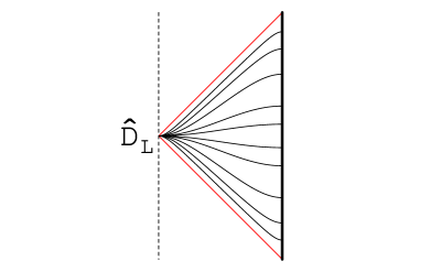
Figure 1: A conformal diagram of the extreme BTZ black hole, with lines of constant BTZ coordinate $t$ (see equation 1) drawn for later reference. Each point on the diagram represents an $S^{1}$ in the spacetime which is the orbit of a spacelike Killing field. The diagonal lines are the horizon, the heavy line at right is the conformal boundary at $r=\infty$, the dashed line is the singularity, and the point $\hat{D}_{L}$ marks the internal infinity which forms the ‘end’ of the infinite throat.

Now, the reader may be concerned by the fact that extreme black holes are often described within CFT₀ [1, 2], without the addition of any new degrees of freedom. To avoid confusion, let us point out that one may consider two distinct classes of spacetimes containing extreme black holes: those with an infinite throat (which we address in this paper) and those without. The usual eternal extreme black hole (figure 1) is clearly an example of the first class, as is any spacetime generated from it by sending in small perturbations from its asymptotic boundary.

The other class of spacetimes arises when extreme black holes form dynamically. Of course, this cannot happen by any classical process. Consider, however, a nearly extreme black hole with one asymptotic region (perhaps formed from the collapse of matter). As a result of a thermal fluctuation, such a black hole may decay to extremality, emitting some Hawking radiation in the process. In the semiclassical description, the decay occurs because of a negative flux of energy across the future horizon. Thus one may expect that, before some advanced time $v$, the spacetime is that of a non-extreme black hole. Thus, it has no infinite throat.

A similar dichotomy arises when one compares non-extreme black holes with differing numbers of asymptotic regions (i.e., one vs. two). In that case, one expects the number of such regions to be reflected by differing dual CFTs [5, 6, 7, 8]. It is natural to expect that our two classes of spacetimes, with and without extreme black hole internal infinities, should correspond to two distinct CFTs as well. The class without an infinite throat (but with one asymptotic region) should be described by CFT₀, while, due to the additional boundary conditions needed at the internal infinity, the class with an infinite throat should be described by a larger CFT.

It is of course possible that the infinite throat is simply a red herring (e.g., as suggested in [13, 14, 15] and references therein). However, pushing this model forward may provide insight into the broader issues of black holes and dual degrees of freedom. We are also interested in the relation to entanglement entropy in the context of AdS/CFT [8, 32, 33]. We therefore investigate features associated with the throat of the extreme BTZ black hole below.

Our approach will be to use a simple linear toy model of AdS₃/CFT₂, which was considered implicitly in [34] and then more explicitly in [35]. The model replaces the CFT₂ of [1] by a single real-valued free scalar field on the cylinder. Empty AdS₃ is of course taken to be dual to the vacuum of this CFT. As we remind the reader in section 2, the BTZ black hole [36, 37] can be constructed as a quotient AdS${}_{3}/\Gamma$ of AdS₃, where $\Gamma$ is an appropriately acting discrete group. The boundary of the BTZ black hole is an analogous quotient of the boundary $\partial$AdS₃ of AdS₃. Since the model CFT is linear, there is a natural map which takes the CFT state on the (boundary) spacetime $S^{1}\times\mathbb{R}$ and constructs an associated CFT state on the quotient boundary $S^{1}\times\mathbb{R}/\Gamma$.

In the non-extreme case, the appropriate quotient construction leads to a black hole with two asymptotic regions, and thus with two asymptotic boundaries, each of which is identical to the boundary of pure AdS₃. Here we will reexamine this construction in detail, focussing on the extreme limit. One asymptotic boundary, which we take to be the right boundary, remains intact and is again identical to the boundary of pure AdS₃. Thus, it is natural for a copy of the original CFT to be associated with this boundary. We refer to this copy as CFT_R. Although the second asymptotic region disappears in this limit, we will nevertheless find that the state dual to an extreme black hole lives in a product conformal field theory, CFT${}_{L}\otimes$CFT_R, where CFT_L is associated with the ‘end’ of the infinite throat of the extreme black hole. This internal infinity is a remnant of the second asymptotic boundary of the non-extreme black hole which, as we shall see below, has degenerated to a null circle. As a result, CFT_L has only right-moving degrees of freedom.

The plan of this paper is as follows: Section 2 provides a brief review of the BTZ black hole and sets notation for the rest of this paper. In section 3 we adopt the method of [35] to obtain the dual description of the BTZ black hole for all masses and angular momenta. In particular, section 3.2 elaborates on the extreme BTZ black hole. Finally, we discuss the implications of our results for AdS/CFT in section 4.

2 Review: the BTZ black hole

Recall [36, 37] that the BTZ black hole is a solution to 2+1 dimensional gravity with negative cosmological constant. Outside the horizon, the line element of this solution is given by

$$ds^{2}=-\frac{(r^{2}-r_{+}^{2})(r^{2}-r_{-}^{2})}{r^{2}\ell^{2}}dt^{2}+\frac{r^{2}\ell^{2}}{(r^{2}-r_{+}^{2})(r^{2}-r_{-}^{2})}dr^{2}+r^{2}\left(d\phi+\frac{r_{+}r_{-}}{r^{2}\ell}dt\right)^{2},$$ (1)

from which one notes the presence of Killing horizons at $r_{+},r_{-}$. In the same notation, the mass of the black hole is

$$M =\frac{r_{+}^{2}+r_{-}^{2}}{8\ell^{2}G_{(3)}},$$ (2)

and the angular momentum is

$$J =\frac{r_{+}r_{-}}{4\ell G_{(3)}},$$ (3)

where $G_{(3)}$ is the three-dimensional gravitational constant. Here $r_{+}\geq r_{-}\geq 0$ and $\ell$ is the AdS length scale in the sense of equation (4) below.

Since gravity has no local degrees of freedom in 2+1 dimensions, the BTZ solution is locally just AdS₃. In fact, the BTZ solution may be thought of as the quotient of a certain region in AdS₃ by an appropriate discrete group of isometries. Section 2.1 reviews the bulk aspects of this quotient construction. In section 2.2 we review the quotient of the conformal boundary $\partial$AdS₃ of AdS₃ which will give $\partial$BTZ, the boundary of our BTZ black hole. In both subsections our main focus is a proper description of the extreme limit $r_{+}\rightarrow r_{-}$.

2.1 BTZ as a quotient

We are interested in the description of the BTZ black hole (1) as a quotient of AdS$\phantom{}{}_{3}$ [37]. We remind the reader that AdS$\phantom{}{}_{3}$ is the universal covering space of the surface $\widehat{\rm AdS}\phantom{}_{3}$ defined by the relation

$$-\ell^{2}=-(T^{1})^{2}-(T^{2})^{2}+(X^{1})^{2}+(X^{2})^{2}$$ (4)

in $\mathbb{R}^{2,2}$ with line element:

$$ds^{2}=-(dT^{1})^{2}-(dT^{2})^{2}+(dX^{1})^{2}+(dX^{2})^{2}.$$ (5)

We will use the coordinates $(\rho,t,\theta)$ adopted in [38],

$$T^{1} =\ell\frac{1+\rho^{2}}{1-\rho^{2}}\sin t, T^{2}=\ell\frac{1+\rho^{2}}{1-\rho^{2}}\cos t$$ (6)

$$X^{1} =\ell\frac{2\rho}{1-\rho^{2}}\cos\theta, X^{2}=\ell\frac{2\rho}{1-\rho^{2}}\sin\theta$$ (7)

with $0<\rho<1$ and $-\pi<\theta\leq\pi$. For $\widehat{\rm AdS}\phantom{}_{3}$ we have $-\pi\leq t<\pi$, but we are interested in the universal cover, AdS₃, which has $-\infty<t<\infty$. In such coordinates, the line element becomes

$$ds^{2}=\frac{4\ell^{2}}{1-\rho^{2}}\left(-\frac{1}{4}(1+\rho^{2})^{2}dt^{2}+d\rho^{2}+\rho^{2}d\theta^{2}\right).$$ (8)

After the conformal rescaling

$$d\tilde{s}^{2}=\left(\frac{1-\rho^{2}}{4\ell^{2}}\right)ds^{2},$$ (9)

the boundary ($\rho\to 1$) line element is just that of the standard cylinder

$$d\tilde{s}_{\partial AdS_{3}}^{2}=-dt^{2}+d\theta^{2}.$$ (10)

The six generators of the $SO(2,2)$ isometries of AdS$\phantom{}{}_{3}$ are given by

$$J_{ab}=x_{b}\frac{\partial}{\partial x_{a}}-x_{a}\frac{\partial}{\partial x_{b}}$$ (11)

with $x^{a}\in(T^{1},T^{2},X^{1},X^{2})$. Consider the Killing vector

$$\xi=\frac{r_{+}}{\ell}J_{T^{2},X^{1}}-\frac{r_{-}}{\ell}J_{T^{1},X^{2}}+J_{X^{1},X^{2}}-J_{T^{2},X^{2}}$$ (12)

with $r_{+}\geq r_{-}\geq 0$. The BTZ black hole is obtained by identifying points $P$ in AdS$\phantom{}{}_{3}$ along the orbits of $\xi$ at intervals of Killing parameter $2\pi n$, with $n\in\mathbb{Z}$:

$$P\sim e^{2\pi\xi n}P.$$ (13)

By applying this quotient procedure to the region $\xi^{2}>0$ we obtain a global description of the BTZ black hole. The coordinate transformation relating the coordinates of (1) to (8) on the quotient space can be found in [37, 34]. The geometry of the resulting quotient depends only on the conjugacy class of $\xi$ within SO(2,2). If $r_{+}\neq r_{-}$, one may choose a representative $\xi^{\prime}$ of the conjugacy class of (12) such that

$$\xi^{\prime}=\frac{r_{+}}{\ell}J_{T^{2},X^{1}}-\frac{r_{-}}{\ell}J_{T^{1},X^{2}}.$$ (14)

An explicit coordinate transformation which takes (12) into $(\ref{E:Killingspace_2})$ for $r_{+}\neq r_{-}$ can be found in [37]. The simpler form (14) has the property that $\xi\rightarrow-\xi$ under an inversion of the space directions: $(X_{1},X_{2})\rightarrow(-X_{1},-X_{2})$. As a result, a quotient construction based on (14) is manifestly symmetric under this inversion. However, the representation (14) is not possible for the extreme black holes ($r_{+}=r_{-}$) on which we wish to focus. As a result, we use (12) instead of the simpler (14). In doing so, we note that our parametrization (12) explicitly breaks the $(X_{1},X_{2})\rightarrow(-X_{1},-X_{2})$ symmetry.

The identifications (13) act on the region $\xi^{2}>0$ in AdS$\phantom{}{}_{3}$. Other regions are not considered as they would lead to closed causal curves or to singularities in the quotient space: points in the bulk of AdS with $\xi^{2}=0$ project onto what is termed the singularity of the black hole in [36, 37].

Although AdS₃ is maximally symmetric, the BTZ black hole has only two isometries. To identify them, we note that these descend from the two Killing fields of AdS₃ which commute with $\xi$. One is $\xi$ itself (12), which by construction projects to a spacelike Killing field on the quotient. The second, $\eta$, may be taken to be proportional to the lift of the time translation symmetry of the BTZ black hole. Let us denote the projection of these Killing fields to the BTZ black hole by $\hat{\xi}$ and $\hat{\eta}$. Comparing with (1), we find that $\hat{\xi}=\frac{\partial}{\partial\phi}$ and $\hat{\eta}=\ell\frac{\partial}{\partial t}$ on the BTZ spacetime, while on AdS₃ we find:

$$\eta=-J_{T^{1},T^{2}}+J_{T^{1},X^{1}}-\frac{r_{-}}{\ell}J_{T^{2},X^{1}}+\frac{r_{+}}{\ell}J_{T^{1},X^{2}}.$$ (15)

2.2 The Quotient of the Boundary

As noted in section 1, we will be especially interested in the action of the quotient (13) on the boundary $\partial{\rm AdS}_{3}$ of ${\rm AdS}_{3}$. We now study this action in detail.

It is convenient to introduce null coordinates $u=t+\theta$, and $v=t-\theta$. In terms of these coordinates, the Killing fields take the form

$$\xi= 2\sqrt{1+\Sigma^{2}}\cos\left(\frac{u}{2}\right)\cos\left(\frac{u}{2}-\arctan\Sigma\right)\partial_{u}$$ (16)

$$- 2\sqrt{1+\Delta^{2}}\cos\left(\frac{v}{2}\right)\cos\left(\frac{v}{2}+\arctan\Delta\right)\partial_{v},$$ (17)

$$\eta= 2\sqrt{1+\Sigma^{2}}\cos\left(\frac{u}{2}\right)\cos\left(\frac{u}{2}-\arctan\Sigma\right)\partial_{u}$$ (18)

$$+ 2\sqrt{1+\Delta^{2}}\cos\left(\frac{v}{2}\right)\cos\left(\frac{v}{2}+\arctan\Delta\right)\partial_{v},$$ (19)

on $\partial{\rm AdS}_{3}$, where we have defined $\Sigma=\frac{r_{+}+r_{-}}{\ell}$ and $\Delta=\frac{r_{+}-r_{-}}{\ell}$.

We wish to identify the region in $\partial$AdS₃ where $\xi^{2}\geq 0$, as only this region will project to the boundary of the BTZ black hole. From (16) we have

$$\xi^{2}=4\sqrt{(1+\Delta^{2})(1+\Sigma^{2})}\cos\left(\frac{u}{2}\right)\cos\left(\frac{v}{2}\right)\cos\left(\frac{u}{2}-\arctan\Sigma\right)\cos\left(\frac{v}{2}+\arctan\Delta\right).$$ (20)

It is convenient to write the region with $\xi^{2}>0$ as $D_{R}\cup D_{L}$, where

$$D_{R} =\{-\pi+2\arctan\Sigma<u<\pi,\,-\pi<v<\pi-2\arctan\Delta\}$$ (21)

$$D_{L} =\{\pi<u<\pi+2\arctan\Sigma,\,\pi-2\arctan\Delta<v<\pi\},$$ (22)

together with the images of $D_{R}\cup D_{L}$ under the translations $u\rightarrow u+2\pi n$ and $v\rightarrow v+2\pi n$. For $r_{+}\neq r_{-}$, the quotients $\hat{D}_{R}$ of $D_{R}$ and $\hat{D}_{L}$ of $D_{L}$ form the respective conformal boundaries of the left and right asymptotic regions of the BTZ black hole.

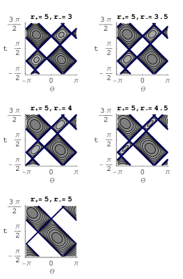
Figure 2: A contour plot of $\xi^{2}$ on the boundary of AdS₃, which under the identification $P\sim e^{2\pi n\xi}P$ becomes the boundary of the BTZ black hole. Regions with $\xi^{2}>0$ are shaded, with darker shading for higher values of $\xi^{2}$. Negative values of $\xi^{2}$ are shaded white. The thick line marks where $\xi^{2}=0$. As the black hole becomes extremal, one boundary collapses to a null line.

It is interesting to note that $D_{L}$ and $D_{R}$ do not appear symmetrically in (21). Indeed, $D_{R}$ is a diamond of coordinate dimensions $(\pi-2\arctan\Sigma)\times(\pi-2\arctan\Delta)$, while $D_{L}$ is a diamond of coordinate dimensions $(2\arctan\Sigma)\times(2\arctan\Delta)$. For $r_{+}\neq r_{-}$, this is a result of our choice of (12) over (14) and the explicit breaking of the symmetry $(X_{1},X_{2})\rightarrow(-X_{1},-X_{2})$. On the other hand, the lack of symmetry is no surprise for extreme black holes (for which $r_{+}=r_{-}$ so that $\Delta=0$), as such black holes have only one asymptotic region.

A plot of the regions $D_{R}$ and $D_{L}$ (in $(t,\theta)$ coordinates) is given in figure 2. One clearly sees that, as the black hole approaches extremality, the left diamond $D_{L}$ collapses to a null line. Despite the fact that $\xi^{2}=0$ on this null line, it is convenient to still refer to it as $D_{L}$. Under the quotient (13) $D_{L}$ maps to a null circle $\hat{D}_{L}$. For $M=0$, $D_{L}$ degenerates to a point, which is in fact a fixed point of (13).

For extreme black holes with $M\neq 0$, we will find in section 3 below that interesting degrees of freedom live on the null circle $\hat{D}_{L}$. As a result, we would like to think of it as part of the boundary of the black hole. In the conformal compactification of AdS₃, the null line $D_{L}$ forms part of the boundary of the region with $\xi^{2}>0$. Curves approaching $D_{L}$ project to curves which travel down the infinite throat of the extreme BTZ black hole. Thus, we may think of this null circle as lying at the end of the throat.

Now, it is clear that $D_{L}$ will not form part of the smooth conformal boundary of the BTZ black hole. However, (see figure 1) there are both spacelike and causal curves (e.g., the generators of the extreme BTZ horizon) which reach $D_{L}$ from within the $\xi^{2}>0$ region. As a result, one should be able to use causal boundary techniques (e.g, [39], which builds on [40, 42, 44, 43, 47, 41, 45, 46, 48]) to give a rigorous sense in which this null circle forms part of the BTZ boundary and to establish in detail its relation to the infinite throat.

3 The dual of the BTZ black hole

As stated in the introduction, our model of AdS/CFT is obtained by replacing the CFT with a theory of a single minimally-coupled massless free scalar field $\phi$ on $S^{1}\times\mathbb{R}$. This model theory is of course conformal, and has central charge $c=1$. The advantage of this model is its linearity, so that the geometric quotient construction of section 2 has a natural analogue in the CFT itself. For simplicity, we also replace the ten dimensional bulk spacetime AdS${}_{3}\times S^{3}\times T^{4}$ with AdS₃. Here we follow [35] and, implicitly, [34] which noted that this simple model is able to reproduce a number of features of the full correspondence such as the energy, angular momentum, and entropy, as well as the more general thermal nature of the BTZ black hole.

In section 2, the BTZ black hole was described as the quotient of AdS₃ by a certain discrete group $\Gamma$, whose action on AdS₃ depends on the mass $M$ and the angular momentum $J$ of the black hole. Similarly, we found that the boundary $\partial$BTZ of the BTZ black hole could be described as the quotient of $D_{L}\cup D_{R}\subset\partial$AdS₃ by the action of $\Gamma$. Now, since the dual CFT is associated with the boundary manifold, $\Gamma$ has a natural action on the CFT as well. If operators on $\partial$BTZ are identified with $\Gamma$-invariant operators on $\partial$AdS₃, the CFT state $|0\rangle$ (dual to empty AdS₃) induces a state $|M,J\rangle$ dual to the BTZ black hole. The state $|M,J\rangle$ is the part of $|0\rangle$ which contains information about those field modes which are periodic under the identifications (13); information about the other field modes is discarded. We will interpret $|M,J\rangle$ as the CFT state dual to the corresponding BTZ black hole.

After addressing the general case in section 3.1, we highlight certain features of the extreme case in section 3.2.

3.1 The general case

As in [35], we shall begin by describing $|0\rangle$ in terms of the lift of modes which are positive frequency on $\partial$BTZ. To do so, we seek solutions of the massless free wave equation on $\partial$AdS₃ which, when restricted to $D_{L}$ and $D_{R}$, are positive frequency with respect to the BTZ time translation symmetry $\eta$. To proceed we introduce null coordinates $\alpha$ and $\beta$ on the BTZ boundary and its covering space $D_{R}\cup D_{L}$, where we require $\alpha$ and $\beta$ to satisfy $\frac{\partial}{\partial\alpha}=\eta+\xi$ , and $\frac{\partial}{\partial\beta}=\eta-\xi$. This determines $\alpha$ and $\beta$ up to constants $\alpha_{0}$ and $\beta_{0}$ in each diamond:

$$\alpha =\frac{\ln\left(\left(\sqrt{1+\Sigma^{2}}\right)\frac{\cos\left(\frac{u}{2}-\arctan(\Sigma)\right)}{\cos\left(\frac{u}{2}\right)}\right)}{\Sigma}+\alpha_{0}, \Sigma\neq 0.$$ (23)

$$\alpha =\tan\left(\frac{u}{2}\right)+\alpha_{0}, \Sigma=0.$$ (24)

$$\beta =-\frac{\ln\left(\left(\sqrt{1+\Delta^{2}}\right)\frac{\cos\left(\frac{v}{2}+\arctan(\Delta)\right)}{\cos\left(\frac{v}{2}\right)}\right)}{\Delta}+\beta_{0}, \Delta\neq 0.$$ (25)

$$\beta =\tan\left(\frac{v}{2}\right)+\beta_{0}, \Delta=0.$$ (26)

We would like our coordinates to be real-valued. In $D_{R}$, the sign of $\cos(u)$ is equal to the sign of $\cos\left(\frac{u}{2}-\arctan\Sigma\right)$, so the argument of the logarithm in (23) is positive and we may take $\alpha_{0}=0$. In contrast, in $D_{L}$, the argument of the logarithm is negative and we may take $\alpha_{0}=-i\frac{\pi}{\Sigma}$, where we have chosen the branch cut of the logarithm in (23) to be in the upper half $u$-plane. Similarly, for $\beta_{0}$, we may take $\beta_{0}=0$ in $D_{R}$ and $\beta_{0}=-i\frac{\pi}{\Sigma}$ in $D_{L}$.

One may use $u_{\omega,+}^{R}=\frac{1}{\sqrt{4\pi\omega}}e^{-i\omega\alpha}$ as a basis for right-moving solutions of the wave equation in $D_{R}$ which are positive frequency with respect to $\eta$, and similarly take $u_{\omega,+}^{L}=\frac{1}{\sqrt{4\pi\omega}}e^{i\omega\alpha}$ as a basis for right-moving solutions of the wave equation in $D_{L}$ which are positive frequency with respect to $\eta$. Note that $\eta$ is future timelike in $D_{R}$ and past timelike in $D_{L}$, while $\xi$ points to the right in $D_{R}$ and to the left in $D_{L}$. In this notation it is easy to see that $\overline{u_{\omega,+}^{L}}$ differs from the analytic continuation of $u_{\omega,+}^{R}$ to $D_{L}$ by a factor of $e^{-\frac{\pi\omega}{\Sigma}}$. A similar statement is true for the left-moving modes $u_{\omega,-}^{L,R}$

Following [49], we may use this observation to express $|0\rangle$ in terms of the state $|0\rangle_{\eta}$ which is the zero-particle state as defined by the modes $u^{R,L}_{\pm}$. To do so, note that for $\omega>0$ the modes

$$W_{\omega,+}^{(1)} =\frac{e^{\frac{\pi\omega}{2\Sigma}}u_{\omega,+}^{R}+e^{-\frac{\pi\omega}{2\Sigma}}\overline{u_{\omega,+}^{L}}}{\sqrt{2\sinh\left(\frac{\pi\omega}{\Sigma}\right)}}, W_{\omega,+}^{(2)}=\frac{e^{\frac{\pi\omega}{2\Sigma}}u_{\omega,+}^{L}+e^{-\frac{\pi\omega}{2\Sigma}}\overline{u_{\omega,+}^{R}}}{\sqrt{2\sinh\left(\frac{\pi\omega}{\Sigma}\right)}},$$ (27)

$$W_{\omega,-}^{(1)} =\frac{e^{\frac{\pi\omega}{2\Delta}}u_{\omega,-}^{R}+e^{-\frac{\pi\omega}{2\Delta}}\overline{u_{\omega,-}^{L}}}{\sqrt{2\sinh\left(\frac{\pi\omega}{\Delta}\right)}}, W_{\omega,-}^{(2)}=\frac{e^{\frac{\pi\omega}{2\Delta}}u_{\omega,-}^{L}+e^{-\frac{\pi\omega}{2\Delta}}\overline{u_{\omega,-}^{R}}}{\sqrt{2\sinh\left(\frac{\pi\omega}{\Delta}\right)}},$$ (28)

are analytic in the lower half imaginary $t$-plane on the complexified boundary of AdS and that they are normalized to have Klein-Gordon norm $\pm 1$. Thus, (27) and (28) are all positive frequency with respect to $t$ on $\partial$AdS₃. Note that these equations remain valid in the limit $\Delta\to 0$ and $\Sigma\to 0$.

We now introduce creation operators $a_{\omega,\pm}^{(1)\dagger}$, $a_{\omega,\pm}^{(2)\dagger}$ for the $W$-modes, along with the corresponding annihilation operators $a_{\omega,\pm}^{(1)}$, $a_{\omega,\pm}^{(2)}$. We also introduce creation operators $b_{\omega,\pm}^{(1)\dagger}$, $b_{\omega,\pm}^{(2)\dagger}$ and annihilation operators $b_{\omega,\pm}^{(1)}$, $b_{\omega,\pm}^{(2)}$ associated with the $u$-modes, which are positive frequency with respect to $\eta$. The relations between these operators may be read directly from (27) and (28):

$$a_{\omega,+}^{(1)} =\frac{e^{\frac{\pi\omega}{2\Sigma}}b_{\omega,+}^{R}-e^{-\frac{\pi\omega}{2\Sigma}}{b^{L\,\dagger}_{\omega,+}}}{\sqrt{2\sinh\left(\frac{\pi\omega}{\Sigma}\right)}}, a_{\omega,+}^{(2)}=\frac{e^{\frac{\pi\omega}{2\Sigma}}b_{\omega,+}^{L}-e^{-\frac{\pi\omega}{2\Sigma}}{b^{R\,\dagger}_{\omega,+}}}{\sqrt{2\sinh\left(\frac{\pi\omega}{\Sigma}\right)}},$$ (29)

$$a_{\omega,-}^{(1)} =\frac{e^{\frac{\pi\omega}{2\Delta}}b_{\omega,-}^{R}-e^{-\frac{\pi\omega}{2\Delta}}{b^{L\,\dagger}_{\omega,-}}}{\sqrt{2\sinh\left(\frac{\pi\omega}{\Delta}\right)}}, a_{\omega,-}^{(2)}=\frac{e^{\frac{\pi\omega}{2\Delta}}u_{\omega,-}^{L}-e^{-\frac{\pi\omega}{2\Delta}}{b^{R\,\dagger}_{\omega,-}}}{\sqrt{2\sinh\left(\frac{\pi\omega}{\Delta}\right)}}.$$ (30)

Recall that $|0\rangle$ is the vacuum on $\partial$AdS₃. This means that $|0\rangle$ is the minimum energy state with respect to the time translation $\frac{\partial}{\partial t}$ on $\partial$AdS₃. As such, it is annihilated by $a_{\omega,\pm}^{(1)}$, $a_{\omega,\pm}^{(2)}$. We will also be interested in the state $|0\rangle_{\eta}$ on $\partial$AdS₃ which is annihilated by $b_{\omega,\pm}^{(1)}$, $b_{\omega,\pm}^{(2)}$. The state $|0\rangle_{\eta}$ induces a state $|M,J\rangle_{\eta}$ on $\partial$BTZ via the identification (13). Because $|M,J\rangle_{\eta}$ is annihilated by $b^{(1)}_{\omega,\pm}$, $b^{(2)}_{\omega,\pm}$ we may identify it as the vacuum state on $\partial$BTZ.

If we express $|0\rangle$ as a set of excitations over $|0\rangle_{\eta}$ on $\partial$AdS₃, then the expression for $|M,J\rangle$ as a set of excitations over $|M,J\rangle_{\eta}$ will follow immediately. Of course, the expression for $|0\rangle$ as a set of excitations over $|0\rangle_{\eta}$ is just the usual Bogoliubov transformation (see e.g. [50, 51, 52, 53]):

$$|0\rangle=e^{-i(K_{+}+K_{-})}|0\rangle_{\eta}$$ (31)

with

$$K_{\epsilon}=i\int_{0}^{\infty}r_{\omega,\epsilon}({b^{R}_{\omega,\epsilon}}^{\dagger}{b^{L}_{\omega,\epsilon}}^{\dagger}-{b^{R}_{\omega,\epsilon}}{b^{L}_{\omega,\epsilon}})d\omega,\quad\text{and~{}}\epsilon=+\ {\rm or}\ -,$$ (32)

where $\tanh(r_{\omega,+})=e^{-\frac{\pi\omega}{\Sigma}}$ and $\tanh(r_{\omega,-})=e^{-\frac{\pi\omega}{\Delta}}$.

It is natural to write

$$|0\rangle_{\eta}=\left(|0\rangle_{R+}\otimes|0\rangle_{L+}\right)\otimes\left(|0\rangle_{R-}\otimes|0\rangle_{L-}\right),$$ (33)

making use of the decomposition into right- and left-moving modes ($+$ or $-$) supported separately on $D_{R}$ or $D_{L}$. We may then rewrite (31) as

$$|0\rangle_{b}=\left(e^{-iK_{+}}|0\rangle_{R,+}|0\rangle_{L,+}\right)\left(e^{-iK_{-}}|0\rangle_{R,-}|0\rangle_{L,-}\right).$$ (34)

We see that the right and left movers are entangled with their partners on the opposite boundary component, but that right-moving and left-moving particles on the same boundary are not entangled with each other. Thus, tracing over, say, all left-moving modes would yield a pure state.

After the identification (13), one finds

$$|M,J\rangle=e^{-i(\tilde{K}_{+}+\tilde{K}_{-})}|M,J\rangle_{\eta},$$ (35)

where $\tilde{K}_{\pm}$ is defined as in (32) but with the integral over $\omega$ replaced by a sum over the discrete frequencies $\omega_{n}=2\pi n$. We may further write $|M,J\rangle_{\eta}=|0\rangle_{L}|0\rangle_{R}$ such that each of the states $|0\rangle_{L}$ and $|0\rangle_{R}$ is the vacuum of a scalar field on $\mathbb{R}\times S^{1}$ (i.e., each is a copy of $|0\rangle$ on $\partial$AdS₃). The states $|0\rangle_{R}$ and $|0\rangle_{L}$ are associated respectively with $\hat{D}_{L}$ and $\hat{D}_{R}$.

An examination of (35) shows that both the right- and left- movers are in thermal states, though with different effective temperatures. The right movers ($\epsilon=+$) have an effective inverse temperature $\beta_{+}=\frac{2\pi}{\Sigma}$, while the left movers have an effective inverse temperature $\beta_{-}=\frac{2\pi}{\Delta}$. This may also be expressed in terms of the physical inverse temperature $\beta$ and a chemical potential $\Omega$ for angular momentum. Such parameters ($\beta,\Omega$) are related to $\beta_{\pm}$ through $\beta_{\pm}=\beta\pm\Omega\beta$. Thus, we have $\Omega=-\frac{r_{-}}{r_{+}}$ and $\beta=\frac{2\pi\ell r_{+}}{r_{+}^{2}-r_{-}^{2}}$. The quantum state of the zero-modes may be treated similarly [35], and again takes the form of a thermo-field double [54] with temperature $\beta=\frac{2\pi\ell r_{+}}{r_{+}^{2}-r_{-}^{2}}$.

Finally, consider the “high temperature limit” where either $T_{+}=1/\beta_{+}\gg 1$ or $T_{-}=1/\beta_{-}\gg 1$. As in [34, 35], one readily shows that the quantum state $|M,J\rangle$ reproduces the mass, angular momentum, and entropy of the BTZ black hole in this limit so long as one takes into account the central charge $c=6Q_{1}Q_{5}=3\ell/2G_{(3)}$ of the CFT₂ of [1]. If one also takes into account the well-known “fractionization” effect of the full CFT₂, then this analysis is valid whenever $T_{+}\gg 1/c$ or $T_{-}\gg 1/c$; i.e., for all black holes larger than the Planck scale ($r_{+}\gg G_{(3)}$).

3.2 The extremal limit

Let us now consider the ($M\neq 0$) extremal limit, $r_{+}\to r_{-}$. Note that the temperature approaches zero while the chemical potential approaches $-1$ , so that the overall effective temperature of the right movers remains finite ($T_{+}=\frac{1}{\beta_{+}}=\frac{1}{(1+\Omega)\beta}$), while that of the left movers vanishes ($T_{-}=\frac{1}{\beta_{-}}=\frac{1}{(1-\Omega)\beta}$).

Our dual description of the extreme black hole remains a state in the product theory CFT${}_{L}\otimes$CFT_R with CFT_R,L associated to $\hat{D}_{R,L}$. Note that CFT_R is a copy of the CFT associated with the boundary of AdS₃. On the other hand, CFT_L arises from the degenerate $D_{L}$, which is a single null line. Thus, CFT_L lives on a one-dimensional null circle and has no left-moving degrees of freedom. As noted above, this null circle lies in some sense at the bottom of the infinite throat of the extreme black hole. The right-movers of CFT_R and CFT_L are entangled in the familiar “thermo-field double” state [54] at temperature $\beta_{+}$, while the left-movers are in their vacuum states.

It is also interesting to consider the BTZ black hole with $M=0$, obtained by taking $r_{+},r_{-}\rightarrow 0$. We find that the effective temperature on both boundaries vanishes and that the dual state is no longer entangled. Instead, we have $|0\rangle=|0\rangle_{\eta}$ where again $|0\rangle_{\eta}=|0\rangle_{L}|0\rangle_{R}$. Now, however, $|0\rangle_{L}$ is the vacuum of the CFT corresponding to the point to which $D_{L}$ collapsed. Note that despite the fact that $D_{L}$ has degenerated to a point, the state $|0\rangle$ could, in principle, have contained non-tivial information about the zero-mode on $D_{L}$.

4 Discussion

In order to investigate the AdS/CFT description of spacetimes with an infinite throat, we analyzed the dual description of the extreme BTZ black hole in a simple toy model. At least in the context of our model, we find that the end of the infinite throat plays a role analogous to that of a second asymptotic region [55, 34, 8, 9, 33, 10]: the CFT state dual to an extremal BTZ black hole lives in a product theory of the form CFT${}_{R}\otimes$CFT_L.

Hence, it appears that the eternal extreme black holes may typify a new class of spacetimes of interest for AdS/CFT. In addition to the traditional choice of a single asymptotic region resembling the conformal boundary of AdS₃ (and described by a single CFT), and also in addition to the case with two such asymptotic regions studied in [55, 34, 35, 8, 33, 10, 32] (plausibly described by a product of two CFTs), one may also consider cases with two inequivalent boundary components. Here we take one component to be a copy of the boundary of AdS₃, while the other is a single null circle which must sit at the bottom of some infinite throat. The suggestion here is that this third class of boundary conditions may again be associated with a product CFT${}_{L}\otimes$CFT_R, where CFT_L contains only, say, right-moving degrees of freedom. In such a setting the extreme black hole may be described as the particular entangled state discussed in section 3.2.

Further investigation of this idea is certainly needed. For example, since the null circle is attached to the bulk in a manner entirely different from that of the conformal boundary in the asymptotic region, it is important to study the possible boundary conditions on this null circle and their influence on the bulk spacetime.

In addition, it is evident that the relation between boundary degrees of freedom and those of the bulk will not be as direct as in the case of conformal boundaries. In this more familiar context, at least in the limit where the bulk fields may be treated semi-classically, one finds [56, 57, 58, 59, 60, 61, 62, 63] that local operators in the dual CFT are essentially (rescaled) boundary limits of local bulk operators. But this seems unlikely to be the case for our internal infinity, as one may see by studying quantum field theory on the extreme black hole background.

Consider, for example, a calculation of the bulk state of a linear quantum field theory on the BTZ background via the same quotient methods applied to the boundary in section 3. Note that this calculation essentially reduces to calculating the two-point function $G$, and that $G$ is related to the two-point function $G_{0}$ of the vacuum over AdS₃ through a sum over images. Furthermore, because this image sum can be performed on the complexified geometry, analyticity of $G_{0}$ guarantees that $G$ will satisfy a KMS condition (see e.g. [64, 65]) with respect to the Killing field which generates the BTZ horizon. As a result, this quantum state will be precisely thermal, and in particular, mixed with respect to observables localized in one exterior region. The thermal ensemble will again be characterized by the right- and left-moving inverse temperatures $\beta_{\pm}$.

Taking the extreme limit, the associated state on the extreme BTZ background will contain thermal excitations of modes with positive angular momentum and, as a result, will again be a mixed state. Thus, studying limits of bulk operators near the end of the infinite throat will reveal no correlations of the sort entangling CFT_L and CFT_R in our dual CFT state.

One might restate this obseveration more physically by noting that the Hartle-Hawking state of the non-extreme black hole (with two asymptotic regions) is an entangled state with respect to modes localized in each of its asymptotic regions. These regions are connected by an Einstein-Rosen bridge. This bridge becomes infinitely long in the extreme limit: one side of the bridge disappears from the spacetime. Thus, there are no longer any modes with which to purify the mixed state seen by an observer at the remaining end of the bridge. Instead, the complete perturbative bulk state is mixed for extreme black holes and, from this point of view, boundary limits of bulk fields do not result in the sort of entanglement described in section 3.2.

A related issue is whether there might be some bulk sense in which the extreme Hartle-Hawking state can be purified through entanglement. We leave further investigation of the connection between our CFT_L and bulk degrees of freedom for future work.

Finally, although no entanglement is obvious from the bulk perspective, it is interesting to note that the description of the CFT as a product CFT${}_{L}\otimes$CFT_R is consistent with the entanglement interpretation of black hole entropy. Such an interpretation remains mysterious for black holes whose dual lives in a single CFT but (as emphasized in [33]) it becomes natural if the dual theory takes a product form as above. In particular, it was advocated in [33] that the entropy of a two-asymptotic-region black hole may always be interpreted as entanglement entropy of its CFT dual. Here, we see the same behavior for black holes with one asymptotic region and an internal infinity. In particular, we note that $|M,J\rangle$ encodes the Bekenstein-Hawking entropy through entanglement.

- [1] J. M. Maldacena, “The large N limit of superconformal field theories and supergravity,” Adv. Theor. Math. Phys. 2, 231 (1998) [Int. J. Theor. Phys. 38, 1113 (1999)] [arXiv:hep-th/9711200].
- [2] O. Aharony, S. S. Gubser, J. M. Maldacena, H. Ooguri and Y. Oz, “Large N field theories, string theory and gravity,” Phys. Rept. 323, 183 (2000) [arXiv:hep-th/9905111].
- [3] A. Strominger and C. Vafa, “Microscopic Origin of the Bekenstein-Hawking Entropy,” Phys. Lett. B 379, 99 (1996) [arXiv:hep-th/9601029].
- [4] T. Jacobson, arXiv:gr-qc/9908031.
- [5] G. T. Horowitz and D. Marolf, “A new approach to string cosmology,” JHEP 9807, 014 (1998) [arXiv:hep-th/9805207].
- [6] V. Balasubramanian, P. Kraus, A. E. Lawrence and S. P. Trivedi, “Holographic probes of anti-de Sitter space-times,” Phys. Rev. D 59, 104021 (1999) [arXiv:hep-th/9808017].
- [7] B. G. Carneiro da Cunha, “Inflation and holography in string theory,” Phys. Rev. D 65, 026001 (2002) [arXiv:hep-th/0105219].
- [8] J. M. Maldacena, “Eternal black holes in Anti-de-Sitter,” JHEP 0304, 021 (2003) [arXiv:hep-th/0106112].
- [9] P. Kraus, H. Ooguri and S. Shenker, “Inside the horizon with AdS/CFT,” Phys. Rev. D 67, 124022 (2003) [arXiv:hep-th/0212277].
- [10] B. Freivogel, V. E. Hubeny, A. Maloney, R. Myers, M. Rangamani and S. Shenker, “Inflation in AdS/CFT,” arXiv:hep-th/0510046.
- [11] See for example S. Hawking and G. F. R. Ellis, “The large scale structure of space-time”, Cambridge University Press 1973, Cambridge, U.K. or P. K. Townsend “Black holes,” [arXiv:gr-qc/9504028]
- [12] W. Israel, “Thermo Field Dynamics Of Black Holes,” Phys. Lett. A 57, 107 (1976).
- [13] A. Sen, “Extremal black holes and elementary string states,” Nucl. Phys. Proc. Suppl. 46, 198 (1996).
- [14] O. Lunin and S. D. Mathur, “Statistical interpretation of Bekenstein entropy for systems with a stretched horizon,” Phys. Rev. Lett. 88, 211303 (2002) [arXiv:hep-th/0202072].
- [15] S. D. Mathur, “The quantum structure of black holes,” arXiv:hep-th/0510180.
- [16] L. Bombelli, R. K. Koul, J. H. Lee and R. D. Sorkin, “A Quantum Source Of Entropy For Black Holes,” Phys. Rev. D 34, 373 (1986).
- [17] M. Srednicki, “Entropy and area,” Phys. Rev. Lett. 71, 666 (1993) [arXiv:hep-th/9303048].
- [18] D. Kabat and M. J. Strassler, Phys. Lett. B329, 46 (1994), [hep-th/9401125].
- [19] C. Holzhey, F. Larsen and F. Wilczek, Nucl. Phys. B424, 443 (1994), [hep-th/9403108].
- [20] T. Jacobson, arXiv:gr-qc/9404039.
- [21] T. Jacobson, Phys. Rev. D50, 6031 (1994), [gr-qc/9407022].
- [22] D. Kabat, Nucl. Phys. B 453, 281 (1995) [arXiv:hep-th/9503016].
- [23] F. Larsen and F. Wilczek, Nucl. Phys. B 458, 249 (1996) [arXiv:hep-th/9506066].
- [24] V. P. Frolov and D. V. Fursaev, Class. Quant. Grav. 15, 2041 (1998) [arXiv:hep-th/9802010].
- [25] H. Casini, Class. Quant. Grav. 21, 2351 (2004) [arXiv:hep-th/0312238].
- [26] A. Yarom and R. Brustein, Nucl. Phys. B 709, 391 (2005) [arXiv:hep-th/0401081].
- [27] M. Cramer, J. Eisert, M. B. Plenio and J. Dreissig, arXiv:quant-ph/0505092.
- [28] R. M. Wald, “The thermodynamics of black holes,” Living Rev. Rel. 4, 6 (2001) [arXiv:gr-qc/9912119].
- [29] R. D. Sorkin, “How wrinkled is the surface of a black hole?,” arXiv:gr-qc/9701056.
- [30] D. Marolf, “On the quantum width of a black hole horizon,” arXiv:hep-th/0312059.
- [31] T. Jacobson, D. Marolf, and C. Rovelli, “Black Hole Entropy: Inside or out?” Int. Journ. Theor. Phys. 44 1907 (2005) [arxiv:hep-th/0501103].
- [32] S. Hawking, J. M. Maldacena and A. Strominger, JHEP 0105, 001 (2001) [arXiv:hep-th/0002145].
- [33] R. Brustein, M. B. Einhorn and A. Yarom, “Entanglement interpretation of black hole entropy in string theory,” arXiv:hep-th/0508217.
- [34] J. M. Maldacena and A. Strominger, “AdS(3) black holes and a stringy exclusion principle,” JHEP 9812, 005 (1998) [arXiv:hep-th/9804085].
- [35] J. Louko and D. Marolf, “Single-exterior black holes and the AdS-CFT conjecture,” Phys. Rev. D 59, 066002 (1999) [arXiv:hep-th/9808081].
- [36] M. Banados, C. Teitelboim and J. Zanelli, “The Black hole in three-dimensional space-time,” Phys. Rev. Lett. 69, 1849 (1992) [arXiv:hep-th/9204099].
- [37] M. Banados, M. Henneaux, C. Teitelboim and J. Zanelli, “Geometry of the (2+1) black hole,” Phys. Rev. D 48, 1506 (1993) [arXiv:gr-qc/9302012].
- [38] S. Aminneborg, I. Bengtsson, D. Brill, S. Holst and P. Peldan, “Black holes and wormholes in 2+1 dimensions,” Class. Quant. Grav. 15, 627 (1998) [arXiv:gr-qc/9707036].
- [39] D. Marolf and S. F. Ross, “A new recipe for causal completions,” Class. Quant. Grav. 20, 4085 (2003) [arXiv:gr-qc/0303025].
- [40] R. Geroch, E. H. Kronheimer, and R. Penrose, “Ideal points in space-time,” Proc. Roy. Soc. Lond. A 327 (1972) 545.
- [41] R. Budic and R. K. Sachs, “Causal boundaries for general relativistic space-times,” J. Math. Phys. 15 (1974) 1302.
- [42] Kuang zhi-quan, Li jian-zeng and Liang can-bin, “-boundary of Taub’s plane-symmetric static vacuum spacetime,” Phys. Rev. D 33 (1986) 1533.
- [43] I. Rácz, “Causal boundary of space-times,” Phys. Rev. D 36 (1987) 1673; ibid, “Causal boundary for stably causal space-times,” Gen. Rel. Grav. 20 (1988) 893.
- [44] Kuang zhi-quan and Liang can-bin, “On the GKP and BS constructions of the -boundary,” J. Math. Phys. 29 (1988) 433.
- [45] L. Szabados, “Causal boundary for strongly causal space-time,” Class. Quant. Grav. 5 (1988) 121;
- [46] L. Szabados, “Causal boundary for strongly causal space-time II,” Class. Quant. Grav. 6 (1989) 77.
- [47] Kuang zhi-quan and Liang can-bin, “On the Rácz and Szabados constructions of the -boundary,” Phys. Rev. D 46 (1992) 4253
- [48] A. Garcia-Parrado and J. M. Senovilla, “Causal relationship: A new tool for the causal characterization of Lorentzian manifolds,” arXiv:gr-qc/0207110.
- [49] W. G. Unruh, “Notes on Black Hole Evaporation,” Phys. Rev. D 14, 870 (1976).
- [50] N. D. Birrell and P. C. W. Davies, Quantum Fields in Curved Space (Cambridge University Press, Cambridge, England, 1982).
- [51] R. M. Wald, Quantum Field Theory in Curved Spacetime and Black Hole Thermodynamics (The University of Chicago Press, Chicago, 1994).
- [52] “Introduction to quantum fields in curved spacetime and the Hawking effect,” arXiv:gr-qc/0308048.
- [53] S. F. Ross, “Black hole thermodynamics,” arXiv:hep-th/0502195.
- [54] Y. Takahashi and H. Umezawa, Collective phenomenon 2 (1975), 55.
- [55] G. T. Horowitz and D. Marolf, “Quantum probes of space-time singularities,” Phys. Rev. D 52, 5670 (1995) [arXiv:gr-qc/9504028].
- [56] S. S. Gubser, I. R. Klebanov and A. M. Polyakov, “Gauge theory correlators from non-critical string theory,” Phys. Lett. B 428, 105 (1998) [arXiv:hep-th/9802109].
- [57] E. Witten, “Anti-de Sitter space and holography,” Adv. Theor. Math. Phys. 2, 253 (1998) [arXiv:hep-th/9802150].
- [58] V. Balasubramanian, P. Kraus and A. E. Lawrence, “Bulk vs. boundary dynamics in anti-de Sitter spacetime,” Phys. Rev. D 59, 046003 (1999) [arXiv:hep-th/9805171].
- [59] V. Balasubramanian, P. Kraus, A. E. Lawrence and S. P. Trivedi, “Holographic probes of anti-de Sitter space-times,” Phys. Rev. D 59, 104021 (1999) [arXiv:hep-th/9808017].
- [60] K. H. Rehren, “Algebraic holography,” Annales Henri Poincare 1, 607 (2000) [arXiv:hep-th/9905179];
- [61] K. H. Rehren, “Local quantum observables in the anti-deSitter - conformal QFT correspondence,” Phys. Lett. B 493, 383 (2000) [arXiv:hep-th/0003120].
- [62] K. H. Rehren, “QFT Lectures on AdS-CFT,” arXiv:hep-th/0411086.
- [63] D. Marolf, “States and boundary terms: Subtleties of Lorentzian AdS/CFT,” JHEP 0505, 042 (2005) [arXiv:hep-th/0412032].
- [64] B.S. Kay, “Purification of KMS states,” Helv. Phys. Acta 58 1030 1040 (1985).
- [65] S.A. Fulling and S.N.M. Ruijsenaars, “Temperature, periodicity and horizons,” Phys. Rep. 152 135 176 (1987).
- [66] B. S. Kay and R. M. Wald, “Theorems On The Uniqueness And Thermal Properties Of Stationary, Nonsingular, Quasifree States On Space-Times With A Bifurcate Killing Horizon,” Phys. Rept. 207, 49 (1991).