Boundary state in open string channel and open/closed string field theory

H. Isono and Y. MatsuoOpen boundary state and string field theory

Hiroshi Isono1, 1

1

We generalize the idea of boundary states to open string channel. They describe the emission and absorption of the open string in the presence of intersecting D-branes. We study the algebra between such states under the star products of string field theory and confirm that they are projectors in a generalized sense. Based on this observation, we propose a modular dual description of Witten’s open string field theory which seems to be an appropriate set-up to study D-branes by string field theory.

1 Introduction

It is almost needless to emphasize the importance of D-branes in understanding the nonperturbative dynamics in string theory. They are essential to the study of the strong gravity region where the coupling constant becomes strong, for example, near the horizon of black holes or the vicinity of time-like big-bang singularity.

D-branes are also useful since we can treat them exactly from 2D conformal field theory. They are described by boundary states $|B^{c}\rangle$ in the closed string channel[1]. They are characterized by,

$$T_{\sigma\tau}|B^{c}\rangle=0$$ (1)

or in the Fourier modes of Virasoro algebra,

$$(L_{n}-\tilde{L}_{-n})|B^{c}\rangle=0\,.$$ (2)

The suffix $c$ is attached to indicate that it belongs to closed string Hilbert space. There are a large amount of references where various properties of such states were studied.

As far as we know, the boundary state condition (1) is considered only in the closed string channel. It is natural in a sense that D-brane plays as a source of emission/absorption of closed string and the boundary state describes such a process. For example, an inner product between boundary states, $\langle B^{c}|q^{L_{0}+\tilde{L}_{0}}|B^{c}\rangle$, describes closed string propagation between D-branes. As we shall see below, however, it is actually possible to consider a similar process for the open strings.

We consider the situation where two D-branes $\Lambda$ and $\Sigma$ intersect each other.

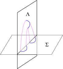
Figure 1: An open string on D-brane $\Lambda$ is created/absorbed on another D-brane $\Sigma$

One may consider a physical process (1) an open string on D-brane $\Lambda$ is emitted from D-brane $\Sigma$, (2) it propagates on the world volume of $\Lambda$ and, (3) it is absorbed on $\Sigma$ (fig.1). As the closed string amplitude, such a process would be described by an inner product of boundary states as,

$${}_{\Lambda\Lambda}^{(\Sigma)}\langle B^{o}|q^{L_{0}^{(\Lambda\Lambda)}}|B^{o}\rangle^{(\Sigma)}_{\Lambda\Lambda}\,,$$ (3)

where $|B^{o}\rangle^{\Sigma}_{\Lambda\Lambda}$ belongs to the open string Hilbert space with both ends at D-brane $\Lambda$. We will call such states as open boundary states or OBS in short. The first purpose of this paper is to define such states and give basic examples.

One of our motivations to introduce such states is the description of the D-branes from string field theory. From some years ago, there have been considerable efforts in this direction. A proposal which was examined carefully was vacuum string field theory (VSFT)[2], where D-branes are described as the projectors of Witten’s star product. Careful studies, however, revealed that the simple projectors do not correspond to D-branes but we need some modification due to the midpoint singularity.

There has been a proposal which takes exactly the same form but has a different interpretation. In [3], it was proved that the (closed string) boundary state satisfies

$$\Psi\star\Psi=\mathcal{C}\Psi\,$$ (4)

where $\mathcal{C}$ is a pure ghost term with divergent coefficient. The star product $\star$ here is that for closed string and there are two vertices studied rather carefully in the literature [4] [5]. A notable feature of the identity (4) is that it holds for both vertices (up to the coefficient $\mathcal{C}$ on the right hand side). It was argued that this relation is closely connected to the factorization relation in boundary CFT [6] and it is mostly independent of the definition of the vertices and the background as long as the conformal symmetry is maintained. It follows that any sensible boundary state in any consistent background needs to satisfy this nonlinear relation. In this sense, this relation gives a precise definition of D-brane in SFT language.

A difficulty was the interpretation of the result. Since this is closed string field theory, it is rather subtle to consider the tachyon vacuum. In this sense, it is rather hard to apply VSFT like interpretation. Instead of that, combined with the relation for OBS, we show that it is more natural to see them as singular limits of the effective open/closed string field theory which is dual to Witten’s OSFT.

The organization of this note consists of two parts. In the first part, we present the definition of OBS and some relations among them in section 2. We have to mention that the discussion given in this proceeding is rather preliminary. It is clear that the open boundary state is definitely important apart from the interpretation in SFT and deserves an independent research. We will soon give more detailed analysis in a forthcoming paper [7].

In the second part, we focus on the application to VSFT like theory. In section 3, we will show that the OBSs defined in section 2 satisfy the same relation with respect to the open string star products. This is a natural generalization of the relation (4) for the closed string boundary states. We present the explicit computation for light-cone type vertex. We note that a state which coincides with OBS was proposed in [8]. It is introduced as a variant of the projector with respect to Witten-type vertex. Although our definition of OBS has more freedom and the interpretation is different, the proof of the idempotency is basically the same as theirs. The feature that the projector relation holds for various vertices distinguishes OBS from other projectors in Witten’s OSFT such as sliver, butterfly, or identity. In section 4, we describe the modular dual description of Witten’s open string field theory and argue that our projector equations should not be interpreted as the equation for VSFT like scenario but rather as the singular limit of such an effective open/closed string field theory.

2 Construction of open boundary state

General arguments

The definition of the open boundary state can be derived from the closed string sector (2) by the doubling technique. Let us take the energy momentum tensor as the first example. We consider an open world sheet with rectangular shape ($0\leq\sigma\leq 2\pi$, $\tau\geq 0$). We identify the anti-holomorphic part of the energy-momentum tensor as,

$$\bar{T}(\bar{w})=T(2\pi-\bar{w})\,,\quad w=\sigma+i\tau\,.$$ (5)

The combined tensor field $T(w,\bar{w})=T(w)+\bar{T}(\bar{w})$ then satisfies the boundary condition (1) at the boundary $\sigma=0,\pi$. In terms of mode operators, it is equivalent to a replacement $\bar{L}_{n}\rightarrow L_{n}$. The boundary condition at $\tau=0$ is then replaced by a condition to the state,

$$(T(\sigma)-\tilde{T}(-\sigma))|B^{o}\rangle=0$$ (6)

for $0<\sigma<\pi$. This equation has a subtlety at $\sigma=0,\pi$ and for the detail see [7].

In order to define an open boundary state, we have to specify three boundary conditions, two D-branes at $\sigma=0,\pi$ and a D-brane at $\tau=0$. The first two boundary conditions in general are implemented by the doubling (for a generic conformal fields $\phi,\bar{\phi}$),

$$\bar{\phi}_{\alpha}(\bar{w})=(\Lambda_{r})_{\alpha\beta}\phi_{\beta}(2\pi-\bar{w})\,,$$ (7)

and the periodicity of the chiral field $\phi_{\alpha}$ is

$$\phi_{\alpha}(w+2\pi)=G_{\alpha\beta}\phi_{\beta}(w)\,.$$ (8)

The boundary condition at $\sigma=0$ is then specified by,

$$\bar{\phi}_{\alpha}(\overline{i\tau})=(\Lambda_{r}G)_{\alpha\beta}\phi_{\beta}(i\tau)\equiv(\Lambda_{l})_{\alpha\beta}\phi_{\beta}(i\tau)\,.$$ (9)

The boundary condition at $\tau=0$ can be defined similarly as,

$$\bar{\phi}_{\alpha}(\sigma)=(\Sigma_{b})_{\alpha\beta}\phi_{\beta}(\sigma),\quad\sigma\in[0,\pi]$$ (10)

but it is used as a constraint to the boundary states $|B^{o}\rangle_{\Lambda_{l}\Lambda_{r}}^{\Sigma_{b}}$ as,

$$\left(\phi_{\alpha}(2\pi-\sigma)-(\Lambda^{-1}_{r}\Sigma_{b})_{\alpha\beta}\phi_{\beta}(\sigma)\right)|B^{o}\rangle_{\Lambda_{l}\Lambda_{r}}^{\Sigma_{b}}=0\,.$$ (11)

Free bosons

Let us use the free boson system to illustrate these ideas. For a free boson, possible boundary conditions are Neumann and Dirichlet. In terms of $J(w)=\partial X(w)$, they can be written as,

$$J(w)+\epsilon\bar{J}(\bar{w})=0\,,\quad\mbox{at Re}(w)=0\,.$$ (12)

Here $\epsilon=1$ for the Neumann and $\epsilon=-1$ for the Dirichlet boundary condition. In the notation of our general discussion, the reflection matrices are identified as $\Lambda_{r,l}=-\epsilon$. Since $G=\epsilon_{l}\epsilon_{r}$, the chiral field becomes periodic when $\epsilon_{l}=\epsilon_{r}$ and anti-periodic when $\epsilon_{l}=-\epsilon_{r}$. It gives the well-known free boson mode expansions,

$$X^{(NN)}(w,\bar{w}) = \hat{x}-\alpha^{\prime}\hat{p}(w-\bar{w})$$ (13)

$$~{}~{}~{}~{}~{}~{}~{}+i\left(\frac{\alpha^{\prime}}{2}\right)^{1/2}\sum_{m\neq 0}\frac{1}{m}\alpha_{m}(e^{imw}+e^{-imw})\,,$$

$$X^{(DD)}(w,\bar{w}) = x+\frac{y-x}{2\pi}(w+\bar{w})$$ (14)

$$~{}~{}~{}~{}~{}~{}~{}~{}+i\left(\frac{\alpha^{\prime}}{2}\right)^{1/2}\sum_{m\neq 0}\frac{1}{m}\alpha_{m}(e^{imw}-e^{-imw})\,,$$

$$X^{(DN)}(w,\bar{w}) = x+i\left(\frac{\alpha^{\prime}}{2}\right)^{2}\sum_{r\in Z+1/2}\frac{1}{r}\alpha_{r}(e^{irw}-e^{-ir\bar{w}})\,,$$ (15)

$$X^{(ND)}(w,\bar{w}) = x+i\left(\frac{\alpha^{\prime}}{2}\right)^{2}\sum_{r\in Z+1/2}\frac{1}{r}\alpha_{r}(e^{irw}+e^{-ir\bar{w}})\,.$$ (16)

The commutation relations for mode variables are,

$$[\alpha_{n},\alpha_{m}]=n\delta_{n+m,0}\,,\quad[\hat{x},\hat{p}]=i\,.$$ (17)

The condition for the boundary state can be written in similar fashion to the closed string case,

$$\partial_{\tau}X(\sigma,\tau)|_{\tau=0}|B^{o}\rangle=0\ \mbox{(Neumann)}\,,\qquad\partial_{\sigma}X(\sigma,\tau)|_{\tau=0}|B^{o}\rangle=0\ \mbox{(Dirichlet)}\,.$$ (18)

The only difference is the mode expansion depends on the boundary conditions for open strings. We note that there are zero-mode quantum operators only in NN sector.

The open boundary states are obtained by solving (18). The result is written compactly as,

$$|B^{o}\rangle^{\epsilon_{b}}_{\epsilon_{l}\epsilon_{r}} \propto \exp\left(-\epsilon_{l}\epsilon_{b}\sum_{n>0}\frac{1}{2n}\alpha_{-n}^{2}\right)|\mbox{zero mode}\rangle_{\epsilon_{l},\epsilon_{r}}^{\epsilon_{b}}\,.$$ (19)

$\epsilon_{l,r,b}$ describe the boundary conditions at left, right and bottom respectively and $+1$ for Neumann boundary condition and $-1$ for Dirichlet boundary condition. $n$ runs over positive integers when $\epsilon_{l}=\epsilon_{r}$ and half-odd positive integers when $\epsilon_{r}\neq\epsilon_{r}$. The vacuum state $|\mbox{zero mode}\rangle_{\epsilon_{l},\epsilon_{r}}^{\epsilon_{b}}$ is the simple Fock vacuum when $(\epsilon_{l},\epsilon_{r})\neq(+1,+1)$. For $(\epsilon_{l},\epsilon_{r})=(+1,+1)$, we need to prepare the zero mode wave function. An appropriate choice is $|\hat{p}=0\rangle$ for $\epsilon_{b}=1$ and $|\hat{x}=x_{0}\rangle$ for $\epsilon_{b}=-1$.

A consistency check of these states is to calculate the inner product between them and compare it with the usual path integral formula. It gives a disc amplitude where the four sides are specified by various boundary conditions. Although this is a disc diagram, we can expect to have an analogue of the modular invariance. In particular, it should be written as,

$${}_{\Lambda_{r},\Lambda_{l}}^{\Sigma_{t}}\langle B^{o}|q^{L_{0}}|B^{o}\rangle_{\Lambda_{l},\Lambda_{r}}^{\Sigma_{b}}\propto{}_{\Sigma_{b},\Sigma_{t}}^{\Lambda_{r}}\langle B^{o}|\tilde{q}^{L_{0}}|B^{o}\rangle_{\Sigma_{t},\Sigma_{b}}^{\Lambda_{l}}\,,$$ (20)

where $q=e^{\pi it},\tilde{q}=e^{-\pi i/t}$ for a real $t>0$.

For the free case, we can confirm this relation easily. A straightforward computation gives,

$${}^{\epsilon_{t}}_{\epsilon_{r}\epsilon_{l}}\langle B^{o}|q^{L_{0}}|B^{o}\rangle^{\epsilon_{b}}_{\epsilon_{l}\epsilon_{r}}=(\prod_{n>0}(1-\epsilon_{t}\epsilon_{b}q^{2n}))^{-1/2}.$$ (21)

As we have used, $n$ becomes positive integer or half-odd positive number depending on $\epsilon_{l},\epsilon_{r}$. (We need to add zero point energy, zero-mode contribution). Since these expressions can be written in terms of theta functions, (20) reduces to the standard modular transformation law.

One interesting aspect of these computations is that the disc amplitude may have such a modular property. The complication should come from the conformal anomaly, namely the mapping from disc to rectangle through conformal mapping is given by Jacobi’s elliptic function. However, an easier alternative computation comes from the path integral formula. These analyses will be discussed in more detail in [7]. We take the case where all the boundary conditions are Neumann. On the rectangle, $X$ has the mode expansion,

$$X(\sigma,\tau)=\sum_{m,n\geq 0}X_{mn}\cos(m\sigma)\cos(n\tau/t)\,.$$ (22)

We then evaluate the gaussian integration,

$$Z=\int dX_{mn}\exp\left(-\frac{1}{4\pi\alpha^{\prime}}\int d^{2}\sigma(\partial X)^{2}\right)\,.$$ (23)

Plugging the expansion (22) into (23) and performing the gaussian integration over $X_{mn}$, we obtain,

$$Z\propto\prod_{m,n\geq 1}(m^{2}t+n^{2}/t)^{-1/2}\propto\eta(q^{2})^{-1/2}\,.$$ (24)

The computation for other boundary conditions is exactly similar and reproduces (21).

Ghosts

For the discussion of string field theory in the following sections, we need the open boundary state for the reparametrization ghosts. Unlike the Majorana fermions which turn out to be more nontrivial, the open boundary state for the ghost fields can be straightforwardly obtained. The boundary conditions become,

$$(b_{n}-b_{-n})|B^{o}\rangle^{(gh)}=(c_{n}+c_{-n})|B^{o}\rangle^{(gh)}=0\,.$$ (25)

These conditions can be solved immediately as,

$$|B^{0}\rangle^{(gh)}=\exp\left(\sum_{n>0}c_{-n}b_{-n}\right)c_{0}c_{1}|0\rangle^{(gh)}\,,$$ (26)

where $|0\rangle^{(gh)}\rangle$ is the $SL(2,R)$-invariant ghost vacuum. The inner product between the ghost OBS becomes,

$${}^{(gh)}\langle B^{o}|b_{0}q^{L_{0}}|B^{0}\rangle^{(gh)}=\prod_{n=1}^{\infty}(1-q^{n})\,,$$ (27)

which is again the square-root of the annulus amplitude from the ghost sector.

3 Projector equation for OBS

We first mention a role of OBS in string field theory context which is different from the study in other parts. As in the closed string case, it is natural to use it as the source term of string field theory. It can be rewritten in the form,

$$Q\Psi+g\Psi\star\Psi=|B^{o}\rangle\,.$$ (28)

This equation generalizes the Yang-Mills equation in the presence of the source D-brane. We will pass the careful study of this relation in our future publication and will study a different feature of boundary states in the context of string field theory.

In the analogy with closed string field theory [3], we expect that the idempotency relation holds for OBS. In this paper, an explicit computation is made only for light-cone type star product [5]. Computation for Witten type vertex would be similar and was made in [8] for a particular type of OBS.

We first derive the star product of OBSs which have the following form,

$$|\Phi_{r}\rangle=\exp\Biggl{(}\frac{1}{2}a^{(r)\dagger}Ma^{(r)\dagger}+\lambda_{r}a^{(r)\dagger}+c^{(r)\dagger}M_{g}b^{(r)\dagger}\Biggr{)}b^{(r)}_{0}|x_{r}^{i},p_{r}^{\mu};\alpha_{r}\rangle$$ (29)

where $r=1,2$. Note that we have added the anti-ghost zero mode oscillator $b_{0}$ because the physical sector of string fields should belong to the anti-ghost zero mode sector. We take the inner product between 3-string vertex and the tensor product of two bras of OBSs obtained by imposing the reflectors on the kets. By carrying this out we arrive at the following formula by utilizing several formulae in [3],

$$|\Phi_{1}\star\Phi_{2}\rangle = ce^{H_{m}}\mathcal{C}e^{H_{g}}\delta^{D-d}(x_{1}-x_{2})~{}b_{0}|x_{1}^{i},(p_{1}+p_{2})^{\mu};\alpha_{1}+\alpha_{2}\rangle\,.$$ (30)

Here the notation is,

$$c = \textrm{det}(1-\tilde{M}\tilde{N})^{-\frac{1}{2}}\textrm{det}(1-\tilde{N_{g}}\tilde{M_{g}})$$

$$H_{m} = \frac{1}{2}a^{\dagger}\tilde{M}^{33}a^{\dagger}+\tilde{N}^{3}\mathbf{P}a^{\dagger}-\frac{\tau_{0}}{2\alpha_{1}\alpha_{2}\alpha_{3}}\mathbf{P}^{2}$$

$$~{}~{}+\frac{1}{2}\tilde{\lambda}\tilde{N}(1-\tilde{M}\tilde{N})^{-1}\tilde{\lambda}+\frac{1}{2}\mu\tilde{M}(1-\tilde{N}\tilde{M})^{-1}\mu+\tilde{\lambda}(1-\tilde{N}\tilde{M})^{-1}\mu$$

$$H_{g} = c^{\dagger}C^{\frac{1}{2}}\tilde{N}^{33}C^{-\frac{1}{2}}b^{\dagger}+\sigma(1-\tilde{M}_{g}\tilde{N}_{g})^{-1}\tilde{M}_{g}\rho$$ (31)

$$\rho^{r} \equiv \tilde{N}_{g}^{r3}b^{\dagger},~{}~{}\sigma^{r}\equiv c^{\dagger}\tilde{N}_{g}^{3r}.$$

In the derivation of this formula, we don’t use the specific form of $M$ . In this sense this gives the general formula for the star products of the squeezed states of the form (29).

In a similar fashion as [3], we evaluate $H_{m},H_{g},\mathcal{C}$. Since our purpose is to evaluate the star products of OBSs, we set the coefficient matrices $M$ to be $\pm 1$ (unit matrix) and $M_{g}$ to be 1. We can evaluate these terms using the explicit forms of the Neumann functions which are given in [3]. The results are :

$$H_{m}(M=1)=\frac{1}{2}a^{\dagger}a^{\dagger}$$ (32)

$$H_{m}(M=-1)=-\frac{1}{2}a^{\dagger}a^{\dagger}-\mathbf{P}B^{T}a^{\dagger}-\frac{1}{4}\mathbf{P}B^{T}B\mathbf{P}$$ (33)

$$H_{g}(M_{g}=1)=c^{\dagger}b^{\dagger}\,.$$ (34)

The computation here is made for the string with NN boundary condition. In order to calculate the star products of OBSs of different types we should construct the SFT for strings with different boundary conditions from NN.

In the case of $|B^{o}\rangle^{D}_{NN}$, by using (32),(34) we obtain

$$|B^{o}\rangle^{D}_{NN}\star|B^{o}\rangle^{D}_{NN}=c_{D}|B^{o}\rangle^{D}_{NN},$$ (35)

where $c_{D}=V_{D-d}c\frac{\partial}{\partial b_{0}}$ and $V_{D-d}$ is the volume of Dirichlet directions.

In the case of $|B^{o}\rangle^{N}_{NN}$, by using (33),(34) and noting that $\mathbf{P}=0$ we obtain

$$|B^{o}\rangle^{N}_{NN}\star|B^{o}\rangle^{N}_{NN}=c_{N}|B^{o}\rangle^{N}_{NN},$$ (36)

where $c_{N}=c\frac{\partial}{\partial b_{0}}$.

4 A modular dual description of Witten’s OSFT?

In the previous section, we have proved the idempotency of OBS with respect to a specific (light-cone type) open string vertex. If we combine it with the results of [3, 6], however, it is natural to expect that the following generalized relations hold for more generic vertices,

$$|B^{c}\rangle\star|B^{c}\rangle\sim|B^{c}\rangle\,,\quad|B^{o}\rangle\star|B^{o}\rangle\sim|B^{o}\rangle\,,\quad|B^{c}\rangle\star|B^{o}\rangle\sim|B^{o}\rangle\,.$$ (37)

Here $\star$ products are vertices for closed string, open string, and open/closed string field theories. The basic reason that these relations should hold is that the boundary states define how left-mover and right-mover should be attached at every point with specific $\tau$ (world sheet time), namely take the following form,

$$|B\rangle\sim\prod_{\sigma}\delta(X^{L}(\sigma)-X^{R}(\sigma))\,.$$ (38)

On the other hand, the string vertex specifies the local overlap of three (or even more) strings, which can be written schematically as,

$$|V_{3}\rangle=\prod_{a=L,R}\prod_{i<j}\prod_{\sigma_{j}}\delta(X^{a}_{i}(\Theta_{ij}(\sigma_{j}))-X^{a}_{j}(\sigma_{j}))\,,$$ (39)

where $\Theta_{ij}$ is a map from $\sigma$ parameter of $j$-th string to that of $i$-th string where they overlap. By a simple inspection, it is easy to see that (37) holds generally with singular coefficients for more general string vertex considered by M.Kaku [9]. In his proposal, the vertex is not restricted to the midpoint interaction (as Witten’s SFT) and endpoint interaction (as lightcone SFT) but overlap can be changed continuously with extra parameters $\alpha_{i}$ ($i=1,2,3$) which describe the length of overlaps as shown in figure 2.

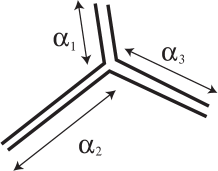
Figure 2: An example of Kaku’s vertex

A natural question is whether these projector equations can be interpreted as equations of motion of some string field theory. If this is possible, it gives the string field theory which is obeyed by D-branes. This question has been considered in [3, 6] in the framework of HIKKO type string field theory and an interpretation similar to VSFT was given. However, it has not been successful in reproducing string diagrams. Especially with only the boundary states in the closed string channel, only the vacuum diagrams are generated in the open string channel. Another drawback is that the numerical coefficient of the kinetic term always diverges and the propagator needs to have a divergent coefficient.

The fact that these identities are satisfied by more general vertices implies that there may be an interpretation which is different from VSFT. Let us recall the most basic feature of diagrams which are generated by Witten’s open string field theory — the existence of the midpoints. The perturbation diagrams are essentially fat diagrams of $\Phi^{3}$ theory whose center is drawn by the midpoint.

In order to describe the boundary degree of freedom, however, it is more natural to see the diagram in a modular dual fashion. Namely the time evolution should be traced from the boundary (fig.3).

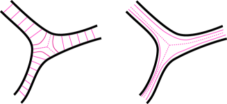
Figure 3: Modular dual picture

In such a dual picture, every strip from the boundary has the same width $\pi/2$ and is attached at the $\Phi^{3}$ diagram drawn by the midpoint. In this dual picture, the external states are the boundary states with time evolution,

$$\Phi=e^{-\pi(L_{0}+\tilde{L}_{0})/2}|B^{c}\rangle_{\alpha},\quad\mbox{or}\quad e^{-\pi L_{0}/2}|B^{o}\rangle_{\alpha}\,.$$ (40)

We note that there is an extra parameter $\alpha$ in order to describe the length of the closed (open) strings. For the open string boundary state attached with the external line, we need to take $\alpha\rightarrow\infty$ limit. These states can be used to construct string amplitude by taking the inner product with “the string vertex” which describes the attachment of these states at the $\Phi^{3}$ graph drawn by the midpoint,

$$A\sim{}_{\alpha_{1},\cdots,\alpha_{N}}\langle V_{N}|\Phi_{1}\rangle_{\alpha_{1}}\cdots|\Phi_{N}\rangle_{\alpha_{N}}\,.$$ (41)

We note that only the planar diagram can be reproduced by such an inner product. In this way, we have arrived at an “effective action” which describes the planar diagrams of Witten’s SFT in the dual channel, (fig.4)

$$\Gamma(\Phi)\sim(\Phi^{o},\Phi^{o})+(\Phi^{c},\Phi^{c})+(\Phi^{o},\Phi^{o},\Phi^{o})+(\Phi^{o},\Phi^{o},\Phi^{c})+(\Phi^{c},\Phi^{c},\Phi^{c})+\cdots\,.$$ (42)

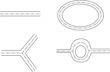
Figure 4: A few diagrams which gives the effective action

We note a few features of such an effective theory,

1. There is no cohomology in the quadratic part $\Phi^{2}$. In this sense, it is similar to VSFT in that it does not generate the usual propagator. However, the interpretation is totally different. This is not the expansion from tachyon vacuum of the existing open or closed SFT. Instead of that, this is simply a re-interpretation of Witten’s open string field theory in the dual channel.

2. The moduli space of string perturbations are generated by the parameters in the vertices instead of the propagator.

3. We need a nonpolynomial action in order to describe all the planar diagrams. This feature resembles nonpolynomial closed string field theory developed in [4].

4. On-shell condition for the external states becomes,

   $$\Phi+\Phi^{2}+\cdots=0$$ (43)

   which is different from (37) in the inclusion of higher nonlinear terms. This is interpreted as the modification due to (40). Such modification is needed anyway to regularize the coefficients appearing in the equation [3].

It is of course rather nontrivial to show explicitly that the modified boundary states (40) satisfy the nonpolynomial equation (43). It is however plausible since this is just the rewriting of the Feynman diagrams of Witten’s open SFT.

Appendix: calculation of the star product

The light-cone type star product is defined by the reflector ${\langle R(1,2)|}$ which maps a ket vector to a bra vector and the three string vertex $|V(1,2,3)\rangle$ which lives in the tensor products of three open string Hilbert spaces:

$$|\Psi_{1}\star\Psi_{2}\rangle_{3} = \int db_{0}^{(1)}db_{0}^{(2)}{}_{1}\langle\Psi_{1}|{}_{2}\langle\Psi_{2}|V(1,2,3)\rangle,$$ (44)

$${}_{2}\langle\Phi| = \int db_{0}{\langle R(1,2)|}\Phi\rangle_{1}.$$ (45)

The reflector is defined by [5]

$${\langle R(1,2)|} \equiv \int d^{d}x^{(1)}d^{d}x^{(2)}\frac{d\alpha_{1}d\alpha_{2}}{(2\pi)^{2}}{}_{1}\langle x^{(1)},\alpha_{1}|{}_{2}\langle x^{(2)},\alpha_{2}|$$ (47)

$$~{}~{}\exp\Biggl{[}\sum_{n\geq 1}(-)^{n+1}\bigl{(}a_{n}^{(1)}a_{n}^{(2)}+c^{(1)}_{n}b^{(2)}_{n}-b^{(1)}_{n}c^{(2)}_{n}\bigr{)}\Biggr{]}$$

$$\times\delta^{d}(x^{(1)}-x^{(2)})\delta(b_{0}^{(1)}-b_{0}^{(2)})2\pi\delta(\alpha_{1}+\alpha_{2}).$$

The three string vertex $|V(1,2,3)\rangle$ is given explicitly in terms of oscillators as:

$${|V(1,2,3)\rangle} \equiv \int~{}\delta(1,2,3)\mu(1,2,3)\prod_{r=1}^{3}\bigl{(}1+\sum_{n=1}^{\infty}\sum_{s=1}^{3}w^{rs}_{n}\alpha_{s}c_{n}^{(s)\dagger}b_{0}^{(r)}\bigr{)}$$ (48)

$$e^{F(1,2,3)}|p_{1},\alpha_{1}\rangle_{1}|p_{2},\alpha_{2}\rangle_{2}|p_{3},\alpha_{3}\rangle_{3},$$

$$F(1,2,3) \equiv \sum_{n,m=1}^{\infty}\sum_{r,s=1}^{3}\tilde{N}^{rs}_{nm}\Biggl{(}\frac{1}{2}a^{(r)\dagger}_{n}a^{(s)\dagger}_{m}+(\sqrt{n}\alpha_{r})c_{n}^{(r)\dagger}(\sqrt{m}\alpha_{s})^{-1}b_{m}^{(s)\dagger}\Biggr{)}$$ (49)

$$+ \sum_{n=1}^{\infty}\sum_{r=1}^{3}\tilde{N}^{r}_{n}a^{(r)\dagger}_{n}\mathbf{P}-\frac{\tau_{0}}{2\alpha_{1}\alpha_{2}\alpha_{3}}\mathbf{P}^{2},$$

$$\int\delta(1,2,3) \equiv \int\frac{d^{d}p_{1}}{(2\pi)^{d}}\frac{d^{d}p_{2}}{(2\pi)^{d}}\frac{d^{d}p_{3}}{(2\pi)^{d}}\frac{d\alpha_{1}}{2\pi}\frac{d\alpha_{2}}{2\pi}\frac{d\alpha_{3}}{2\pi}$$ (50)

$$(2\pi)^{d}\delta^{d}(p_{1}+p_{2}+p_{3})(2\pi)\delta(\alpha_{1}+\alpha_{2}+\alpha_{3}),$$

$$\mathbf{P} \equiv \alpha_{1}p_{2}-\alpha_{2}p_{1},$$ (51)

$$w_{n}^{rs} \equiv \Bigl{(}\chi^{rs}\bar{N}^{s}_{n}+\frac{1}{\alpha_{r}}\sum_{m=1}^{n-1}\bar{N}^{ss}_{n-m,m}\Bigr{)}n,$$ (52)

$$\chi^{rs} \equiv \delta_{r,s}\frac{1}{\alpha_{r}}(\alpha_{r-1}-\alpha_{r+1})+\sum^{3}_{t=1}\epsilon^{rst},$$ (53)

$$\mu(1,2,3) \equiv \exp{\Bigl{(}-\tau_{0}\sum^{3}_{r=1}\frac{1}{\alpha_{r}}\Bigr{)}},\qquad\tau_{0}\equiv\sum^{3}_{r=1}\alpha_{r}\ln|\alpha_{r}|.$$ (54)

We consider the tensor product

$$|\Phi_{1}\rangle\otimes|\Phi_{2}\rangle = \exp\Biggl{(}\frac{1}{2}a\tilde{M}a+\tilde{\lambda}a+c\tilde{M}_{g}b\Biggr{)}\cdot$$ (55)

$$~{}~{}~{}~{}~{}~{}~{}\cdot b^{(1)}_{0}|x_{1}^{i},-p_{1}^{\mu};-\alpha_{1}\rangle\otimes b^{(2)}_{0}|x_{2}^{i},-p_{2}^{\mu};-\alpha_{2}\rangle\,.$$

The corresponding bra state is obtained by applying the reflector,

$$\langle\Phi_{1}|\otimes\langle\Phi_{2}|=\langle x_{1}^{i},-p_{1}^{\mu};-\alpha_{1}|b^{(1)}_{0}\otimes\langle x_{2}^{i},-p_{2}^{\mu};-\alpha_{2}|b^{(2)}_{0}\exp\Biggl{(}\frac{1}{2}a\tilde{M}a+\tilde{\lambda}a-c\tilde{M}_{g}b\Biggr{)}\,,$$ (56)

where

$$a^{\dagger} = \Bigl{(}a^{\mu(1)\dagger}_{n},a^{\mu(2)\dagger}_{n}\Bigr{)}\,,~{}~{}\textrm{similar notation for }c^{\dagger}\textrm{ and }b^{\dagger}$$

$$\tilde{M}_{mn} = (-)^{m+n}M_{mn},~{}~{}(\tilde{M_{g}})_{mn}=(-)^{m+n}(M_{g})_{mn}$$ (57)

$$\tilde{M}^{rs}_{mn} = \left(\begin{array}[]{cc}\tilde{M}_{mn}&0\\ 0&\tilde{M}_{mn}\end{array}\right),\,(\tilde{M}_{g})^{rs}_{mn}=\left(\begin{array}[]{cc}(\tilde{M_{g}})_{mn}&0\\ 0&(\tilde{M_{g}})_{mn}\end{array}\right)$$ (62)

We take the inner product between this bra state and the 3-string vertex. For this purpose, it is convenient to rewrite the factor in the exponential in the vertex as

$$F(1,2,3) \equiv \frac{1}{2}a^{\dagger}\tilde{N}a^{\dagger}+\mu a^{\dagger}-\frac{\tau_{0}}{2\alpha_{1}\alpha_{2}\alpha_{3}}\mathbf{P}^{2}+\frac{1}{2}\sum_{n,m=1}^{\infty}\tilde{N}^{33}_{nm}a_{n}^{(3)\dagger}a_{m}^{(3)\dagger}$$ (63)

$$+\sum^{\infty}_{n=1}\tilde{N}^{3}_{n}a_{n}^{(3)\dagger}\mathbf{P}+c^{\dagger}\tilde{N}_{g}b^{\dagger}+c^{\dagger}\tilde{\rho}+\tilde{\sigma}b^{\dagger}$$

$$+c^{(3)\dagger}C^{\frac{1}{2}}\tilde{N}^{33}C^{-\frac{1}{2}}b^{(3)\dagger}$$

where we introduce some notations

$$\mu^{r} = \tilde{N}^{r}\mathcal{P}+\tilde{N}^{r3}a^{(3)\dagger}$$

$$\tilde{N}_{g}^{rs} = \alpha_{r}C^{\frac{1}{2}}\tilde{N}^{rs}C^{-\frac{1}{2}}\alpha_{s}^{-1}$$

$$\tilde{\sigma}^{r} = c^{(3)\dagger}\alpha_{3}C^{\frac{1}{2}}\tilde{N}^{3r}C^{-\frac{1}{2}}\alpha_{r}^{-1}=c^{(3)\dagger}\tilde{N}_{g}^{3r}$$ (64)

$$\tilde{\rho}^{r} = \alpha_{r}C^{\frac{1}{2}}\tilde{N}^{r3}C^{-\frac{1}{2}}\alpha_{3}^{-1}b^{(3)\dagger}+w^{3r}\alpha_{r}b^{(3)}_{0}=\tilde{N}_{g}^{r3}b^{(3)\dagger}+w^{3r}\alpha_{r}b^{(3)}_{0}$$

By taking the inner product with the aid of the useful formulae [3], we can arrive at (30).

References

- [1] For review articles, for example, P. Di Vecchia and A. Liccardo, NATO Adv. Study Inst. Ser. C. Math. Phys. Sci. 556, 1 (2000) [arXiv:hep-th/9912161]; arXiv:hep-th/9912275.
- [2] L. Rastelli, A. Sen and B. Zwiebach, Adv. Theor. Math. Phys. 5, 353 (2002) [arXiv:hep-th/0012251]; Adv. Theor. Math. Phys. 5, 393 (2002) [arXiv:hep-th/0102112].
- [3] I. Kishimoto, Y. Matsuo and E. Watanabe, Phys. Rev. D 68, 126006 (2003) [arXiv:hep-th/0306189]; Prog. Theor. Phys. 111, 433 (2004) [arXiv:hep-th/0312122].
- [4] M. Saadi and B. Zwiebach, Annals Phys. 192, 213 (1989); T. Kugo, H. Kunitomo and K. Suehiro, Phys. Lett. B 226, 48 (1989).
- [5] H. Hata, K. Itoh, T. Kugo, H. Kunitomo and K. Ogawa, Phys. Rev. D 34, 2360 (1986); Phys. Rev. D 35, 1318 (1987).
- [6] I. Kishimoto and Y. Matsuo, Phys. Lett. B 590, 303 (2004) [arXiv:hep-th/0402107]; Nucl. Phys. B 707, 3 (2005) [arXiv:hep-th/0409069].
- [7] Y. Imamura, H. Isono and Y. Matsuo to appear.
- [8] D. Gaiotto, L. Rastelli, A. Sen and B. Zwiebach, JHEP 0204, 060 (2002) [arXiv:hep-th/0202151].
- [9] M. Kaku, Phys. Lett. B 200, 22 (1988); Int. J. Mod. Phys. A 2, 1 (1987).