Light-front Hamiltonians for heavy quarks and gluons

Abstract

A boost-invariant light-front Hamiltonian formulation of canonical quantum chromodynamics provides a heuristic picture of the binding mechanism for effective heavy quarks and gluons.

1 INTRODUCTION

Light front (LF) Hamiltonian operators for effective particles in quantum field theory (QFT) provide a new path toward understanding of hadronic structure and interactions. The origin of new thrust is a far reaching simplification of the approach in comparison to the standard form of dynamics: boosts are kinematical, instantaneous potentials can exist on the front hyperplane without contradicting the assumption that no physical effect can propagate faster than light, and one can avoid the problem of the vacuum structure. Rotational symmetry is dynamical and poses problems, but we have a lot of intuition about rotational symmetry. It seems simpler to obtain rotational symmetry in the LF Hamiltonian approach than to solve the problem of dynamical boost symmetry or the vacuum problem in the standard approach. The price one has to pay for these gains in the LF Hamiltonian approach is a heavy-duty renormalization group procedure and a scheme to finesse a leading approximation around which one can develop a calculation of corrections. I describe a heuristic picture of binding for heavy quarks and gluons that begins to emerge from application of these tools in QCD. I will focus on results for gluonium and heavy quarkonia.

The binding of quarks and gluons occurs typically above threshold, which means that the sum of masses of the constituents is smaller than the mass of the bound state. How can such effect occur in a relativistic quantum theory? It does not happen in QED. So, how can it happen? A boost-invariant light-front Hamiltonian formulation of QCD provides a heuristic picture in which a binding between heavy effective quarks and gluons may arise above threshold because the eigenvalue condition for a renormalized Hamiltonian operator may include a large positive contribution from mass counterterms that can be compensated by exchange of gluons only in color-singlet states of limited size. One can conceive a subtle calculation without ever worrying about any non-trivial structure in the vacuum. But there is a trick needed to finesse effective interactions: one introduces an ansatz for a gluon mass gap in the Fock states that contain gluons in addition to the dominant sectors. Fortunately, the effective theory is not very sensitive to the ansatz and one can propose a scheme of successive approximations that may in principle replace the gap ansatz order by order with true interactions, “true” meaning implied by the relevant theory. It is encouraging that even the first approximation exhibits a considerable degree of rotational symmetry. The key reference for this talk is [1].

2 KEY POINTS

The framework for building a constituent picture for hadrons using LF Hamiltonians has several ingredients. The whole procedure begins with a canonical Lagrangian of QCD, but the actual Hamiltonian operators one works with are very different from the bare canonical ones.

1. In the momentum range where the binding mechanism works, the coupling constant $\alpha=g^{2}/(4\pi)$ is comparable to 1. By this I mean that the relevant Hamiltonian contains a coupling constant $g$ in its vertices, but the constant is a function of a renormalization group parameter $\lambda$. When $\lambda\rightarrow\infty$, the constant $g$ tends to 0 (it is never 0 for finite $\lambda$). In fact, the entire Hamiltonian as an operator is a function of $\lambda$,

$$H = H_{\lambda}\,.$$ (1)

The point is that one needs a method to find $H_{\lambda}$. In QED, one can try to deduce a Hamiltonian from $S$-matrix theory, guessing potentials from scattering amplitudes within a perturbative expansion for very small coupling constant. In QCD, one expects confinement and if this expectation is taken seriously into account, including the large value of $\alpha$ in the binding mechanism, there is no precise link a la QED between the $S$-matrix for hadrons and quark and gluon forces responsible for the binding phenomenon. In order to develop LF Hamiltonians for quarks and gluons, I will use a renormalization group procedure for effective particles (RGPEP). The RGPEP provides an expression for $H_{\lambda}$ order by order in an expansion in a small coupling without reference to the $S$-matrix for quarks and gluons. It also offers a possibility to extrapolate the small-coupling results to large values of the coupling constant because the extrapolation is for the Hamiltonian operator, not for the observables (see points 5 and 6 below). But the Hamiltonian contains finite parts of the ultraviolet (UV) counterterms that are unknown, and the only possibility to find those unknown finite parts is to consider observables for hadrons, including symmetries such as rotational symmetry in decay amplitudes.

2. The Hamiltonians $H_{\lambda}$ must be clearly related to the canonical theory. The RGPEP equations for evaluating $H_{\lambda}$ in perturbation theory (see e.g. [1]) are based on a unitary change of basis in the space of operators,

$$q_{\lambda} = U_{\lambda}\,q_{can}\,U_{\lambda}^{\dagger}\,,$$ (2)

$$H_{\lambda}(q_{\lambda}) = \left[H_{can}+H_{CT}\right]_{reg}(q_{can})\,.$$ (3)

This is a similar idea to Gell-Mann’s current-constituent relationship [2, 3] studied by Melosh [4], except that now it is built in a dynamical scheme of QCD using RGPEP [5]. The symbol $q_{\lambda}$ stands for creation or annihilation operators for effective quarks and gluons, and $q_{can}$ stands for canonical operators. $H_{can}$ denotes the canonical LF QCD Hamiltonian with a regularization. An admissible regularization must be imposed on the transverse and longitudinal relative momenta of interacting particles, those that are invariant with respect to the Poincaré transformations that do not take four-vectors out of the LF hyperplane $x^{+}=0$. $H_{CT}$ denotes the required counterterms. The RGPEP determines how to find the structure of $H_{CT}$ order by order in perturbation theory. The regularization and renormalization are ab initio in the Hamiltonian, defined en block for the operators in the Fock space that can be built using either $q_{can}$ or $q_{\lambda}$.

3. In principle, a Fock-space decomposition of physical states contains wave functions that extend up to the cutoffs introduced by regularization. Can a Hamiltonian formalism in a Fock space with not explicitly covariant regularization lead to covariant results? When Dirac introduced the front form of dynamics [6], he reduced the problem to finding 10 generators that satisfy the Poincaré algebra:

$$[P^{\mu},P^{\nu}] = 0\,,$$ (4)

$${[}P^{\mu},M^{\nu\rho}] = i(g^{\mu\nu}P^{\rho}-g^{\mu\rho}P^{\nu})\,,$$ (5)

$${[}M^{\mu\nu},M^{\rho\sigma}] = i(g^{\mu\rho}M^{\sigma\nu}-g^{\mu\sigma}M^{\rho\nu}$$ (6)

$$+ g^{\nu\rho}M^{\mu\sigma}-g^{\nu\sigma}M^{\mu\rho})\,.$$

Can one seek such 10 generators in QFT using RGPEP? The seven (one more than in the standard approach) kinematical generators: $P^{+}$, $P^{\perp}$, $M^{+-}$, $M^{+\perp}$, and $J^{3}$, do not require regularization and are the same as in a non-interacting theory. But the three dynamical generators: $H=P^{-}$ and $M^{-\perp}$, require regularization and renormalization. So far, it has only been demonstrated in a scalar theory up to second order in the coupling constant [7] that RGPEP produces a required solution. In that case one obtains commutation relations of the form ($g$ is the charge)

$$[J^{i}_{\lambda},J^{j}_{\lambda}] = i\epsilon_{ijk}J^{k}_{\lambda}+o(g^{3})\,.$$ (7)

There is no reason to expect that the method cannot work to higher orders. Dirac has observed that the challenge of an interacting theory is to unfold the commutators that contain products of interactions. Such products appear in second-order expressions and a solution exists. Fig. 1 illustrates the structure of the first- and second-order terms in the creation operators $a^{\dagger}_{\lambda}$ for effective particles. The zeroth-order term is $a^{\dagger}_{can}$ itself.

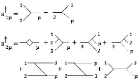
Figure 1: Structure of the first- and second-order terms in $a^{\dagger}_{\lambda}$ in a scalar theory of Ref. [7]. The thick lines on the left-hand sides of the vertices denote canonical creation operators, and on the right-hand sides canonical annihilation operators. The thin lines indicate how the momentum of an effective particle enters the structure.

The Dirac problem in QCD is much more complex than in a scalar model theory. But it cannot be addressed in the RGPEP procedure without better understanding of the effective dynamics described by $H_{\lambda\,QCD}$ because of additional small-$x$ singularities in QCD that are not under control of the UV renormalization group procedure (see below).

4. A method for deriving Hamiltonians $H_{\lambda}$ must produce operators that in the case of extremely small coupling constant must deliver a covariant scattering matrix in perturbation theory. Wiȩckowski [8] settled the issue in a 1-loop example of $\phi^{3}$ theory in 5+1 dimensions, which is asymptotically free (AF) in perturbative sense. His more general theorem states: The same $S$-matrix for scattering of physical particles can be obtained using (1) a bare Hamiltonian $\left[H_{can}+H_{CT}\right]_{reg}$, and representing the in and out particles with creation and annihilation operators $q_{can}$, and (2) an effective Hamiltonian $H_{\lambda}$ and effective operators $q_{\lambda}$. In each order of perturbation theory, the result for the $S$-matrix is the same, provided that the relationship between $q_{can}$ and $q_{\lambda}$, and between initial $H$ and $H_{\lambda}$, is calculated up to this order.

It is important that $H_{\lambda}$ for effective particles contains form factors in interaction terms. Thus, it resembles a non-local theory of the type known in relativistic nuclear physics, where nucleons interact through exchange of mesons. In distinction from the nuclear models, however, $H_{\lambda}$ originates from QFT and the form factors result from a renormalization group procedure. An example of old-fashioned diagrams that contribute to an amplitude of the type $e^{+}e^{-}\rightarrow hadrons$ is shown in Fig. 2.

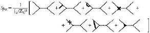
Figure 2: Counterterms found using RGPEP produce a covariant amplitude of the type $e^{+}e^{-}\rightarrow hadrons$, $S_{\beta\alpha}$ for transition from the incoming state $|\alpha\rangle$ to the outgoing state $|\beta\rangle$, in an old-fashioned one-loop calculation with two wave function renormalization factors $1/\sqrt{Z_{q}}$ in front [8].

Note that the integrals over momenta in the loops are limited in a non-covariant way because the momenta are already limited once and for all in a non-covariant way in the Hamiltonian. Nevertheless, the result for the scattering amplitude is the same as obtained using Feynman diagrams because the counterterms were found from RGPEP and all they do is to remove the effects of regularization [8]. This is interesting also from the point of view of the world-sheet program developed by Thorn for planar diagrams [9, 10].

5. How could one calculate bound state masses using $H_{\lambda}$? This can be done like in atomic physics, where the Coulomb potential is only of formal order $e^{2}$ and still describes a giant variety of bound states. As soon as RGPEP produces $H_{\lambda}(g_{\lambda})$, one can tackle the eigenvalue problem for $H_{\lambda}$. A special feature of RGPEP matters here: it works in perturbation theory without ever creating small energy denominators (this feature is built in the design of RGPEP following the principles formulated earlier in [11, 12]). Therefore, as long as $\lambda$ is above the size of momenta that matter in the binding mechanism, the resulting Hamiltonians can provide relatively small matrices, called windows, whose diagonalization produces eigenvalues for the bound states. But the closer one approaches the scale of binding, the higher order calculation is required and the larger is the required coupling constant $g_{\lambda}$. So, the window must be of the right size for the procedure to work. This aspect of the RGPEP scheme was carefully tested numerically in an exactly soluble model with AF [13]. A benchmark method of altered Wegner’s equation [14, 15, 16] produces Fig. 3 which shows how successive orders improve the accuracy of evaluation of the window in terms of its bound-state eigenvalue. Note that the parameter $\lambda$ must be near the scale of binding for a small window to work. The model also indicates that a low order perturbative window, obtained for arbitrarily small coupling (or arbitrarily small $\Lambda_{QCD}$ in the RGPEP scheme) can be extrapolated to realistic values of $g_{\lambda}$ and then the window renders a good approximation for the bound-state eigenvalue of the whole theory. In future, after the boost-invariant RGPEP leads to identification of dominant terms via perturbation theory, the Wegner equation, or an altered version of it, can be applied to calculate window Hamiltonians for large coupling constants in specific cases without using perturbation theory.

6. In the case of QCD, in the effective-particle basis in the Fock space, a gluonium state can be written as

$$\Psi\rangle = |g_{\lambda}g_{\lambda}\rangle+|g_{\lambda}g_{\lambda}g_{\lambda}\rangle+...\,,$$ (8)

and a heavy quarkonium as

$$\Psi\rangle = |Q_{\lambda}\bar{Q}_{\lambda}\rangle+|Q_{\lambda}\bar{Q}_{\lambda}g_{\lambda}\rangle+...\,.$$ (9)

But why should such expansion converge at all, especially when the coupling constant is comparable with 1? The reason is that the growth of $g_{\lambda}$ when $\lambda$ is lowered using RGPEP can be compensated by the narrowing of form factors $f_{\lambda}$ in the interaction vertices. In other words, the interactions in a Hamiltonian with a small $\lambda$ die out so quickly for large energy changes that they are effectively not strong enough to spread probability to sectors with many effective particles, even when the coupling constant itself is large [17]. The form factors of RGPEP solve the problem that the interactions among effective constituents must be strong and at the same time the number of the effective constituents must be small (as indicated by the success of the constituent quark model). The situation is akin to nuclear physics with practically fixed number of nucleons.

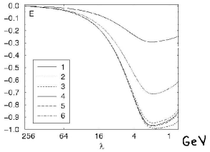
Figure 3: A bound-state calculation in an asymptotically free matrix model: a small window Hamiltonian matrix is evaluated in six successive orders of perturbation theory in RGPEP (using altered Wegner’s flow equation) and then diagonalized non-perturbatively using a computer. The exact bound-state eigenvalue is -1 [13].

7. The next key point is that in order to solve the eigenvalue problem for $H_{\lambda}$ in QCD, one has to truncate it in the number of effective constituents anyway. But in order to do it in a systematically improvable way, I assume that there exists a shift in the energy of gluons due to non-abelian potentials that come out from RGPEP in QCD (there are no such potentials coming out in QED, cf. [18]) and that the shift can be approximated in the form of a mass gap function for gluons. A well-known operation $R$ [19] produces then an effective Hamiltonian in the dominant sectors: two effective gluons in a gluonium, and a pair of effective quarks in a heavy quarkonium. Let me follow Masłowski’s analysis of gluonium [20], as an example of the application of RGPEP (the example is analogous to the quarkonium case described in [1], although gluons demand a more advanced analysis because one cannot employ a non-relativistic approximation to begin with). Matrix elements of the effective Hamiltonian between states of two effective gluons $|g_{\lambda}g_{\lambda}\rangle$ labeled 1 and 2 with relative momentum $k$, are of the form

$$H_{kk^{\prime}}=(E_{k}+E_{CT\,k})\delta_{kk^{\prime}}+W_{kk^{\prime}}$$ (10)

$$+{1\over 2}\sum_{q}Y_{kq}\left[{1\over E_{k0}-E_{q\mu}}+{1\over E_{k^{\prime}0}-E_{q\mu}}\right]Y_{qk^{\prime}},$$

where $E_{k}$ is an eigenvalue of kinetic energy operator $T_{\lambda}$, equal $(k^{\perp\,2}+m_{\lambda}^{2})/(x_{1}x_{2}P^{+})$, $m_{\lambda}$ is the effective mass of gluons in $T_{\lambda}$, $E_{CT}$ is the contribution of the mass counterterm for gluons, $W_{kk^{\prime}}$ is the effective interaction generated by RGPEP, the sum stands for summation over the effective three-gluon basis states that are coupled to the two-gluon basis states by the interaction term $Y$ in $H_{\lambda}$, and $E_{q\mu}$ is the LF energy of the three effective gluons, each of which has a mass gap ansatz $\mu^{2}$ in place of $m_{\lambda}^{2}$. The mass gap depends on the relative momenta of 3 gluons and can be described using a Hamiltonian term

$$T_{\mu}={1\over 3!}\sum_{123}\int[123]\sum_{i=1}^{3}\frac{\mu_{i}^{2}(123)}{p^{+}_{i}}|123\rangle\langle 123|\,,$$ (11)

where $[123]$ means the LF measure in the integration over momenta of the three gluons and the sum extends over their polarizations (only two transverse ones).

8. The trick with the mass gap ansatz is to make it correctable order-by-order according to the following rule [21]. One can write $H_{\lambda}=T+V$ and add and subtract the gap term $T_{\mu}$, changing nothing. But one is free to do it introducing a ratio of the coupling constant to its physically correct value for a $\lambda$ that one finds suitable to work with in this scheme:

$$H_{\lambda} = T+T_{\mu}+\left[V-\left({\alpha_{\lambda}\over\alpha_{physical}}\right)^{2}\,T_{\mu}\right]\,.$$ (12)

For $\alpha_{\lambda}=\alpha_{physical}$, nothing is changed. But in a perturbative expansion for small $\alpha_{\lambda}$, the added term is large while the subtracted term is negligible. This is how one can attempt to incorporate the non-perturbative effects in the three-body sector and couplings to sectors with more effective gluons in the first approximation. The effect of $T_{\mu}$ in second-order calculation of $H_{kk^{\prime}}$ will be replaced by the actual interactions in fourth-order RGPEP calculation plus new small ansatz correction that will be correctable in higher order, and so on. The problem one solves this way is that unless the sector with 3 gluons is separated by a gap from the sector with two gluons, it is not legitimate to use perturbation theory in order to account for the coupling between the sectors. Most probably, in higher order analysis, the ansatz for a gap will be pushed away to sectors with more effective gluons. Nothing can be said for certain yet because the 4th order calculation has not been completed. Note, however, that if the mass gap ansatz approximates the true QCD interactions well, there will be only a little change in the leading, approximate picture associated with transition from the case with the ansatz term $T_{\mu}$ and without the interaction $V-T_{\mu}$ to the case with $V$ and without $T_{\mu}$. But in both cases one can consider extrapolation of the window Hamiltonians in expansion in powers of the coupling $\alpha_{\lambda}$ from arbitrarily small values to $\alpha_{physical}$ that is comparable with 1, since the RGPEP form factors prevent the interactions from blowing up at large momenta for large couplings.

9. How does the binding mechanism work? The mechanism I am talking about can be considered an extension of the seminal work of Lepage and Brodsky [22] to the domain of small momentum transfers. They were working on exclusive processes with a large

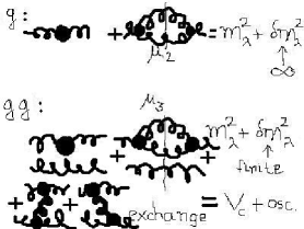
Figure 4: The mechanism of binding above threshold in gluonium. The upper line refers to how the mass counterterm for gluons is fixed using a single-gluon eigenvalue equation for $H_{\lambda}$, and the lower line refers to what happens in the eigenvalue equation for globally colorless states of two effective gluons, see the text. The gluon lines are fat because they represent effective gluons.

momentum transfer using diagrammatic rules for scattering amplitudes, while the RGPEP allows me to consider what happens in the Hamiltonian eigenvalue equation (with a gap ansatz) when the momentum transfer is in the range of the binding mechanism. Of course, Lepage and Brodsky considered usual mesons and I discuss here gluonium, but this is not essential and I will discuss a case of quarkonium later. Let me explain how the binding above threshold emerges using Fig. 4. This is the mechanism that Masłowski used in his calculation [20]. The main difference in comparison with the earlier work of Allen and Perry [23], besides the explicitly perturbative RGPEP which is different from coupling coherence employed by Allen and Perry, is that RGPEP provides a boost-invariant eigenvalue equation for the mass of a gluonium in arbitrary motion, the basis states are built from effective gluons instead of the canonical ones, the form factors strongly limit changes of invariant masses (instead of the changes of $P^{-}$ that are associated in [23] with interaction terms that depend on spectators), and one has to consider the coupling to three-gluon states in order to cancel small-$x$ divergences (3-gluon states could be neglected entirely in [23]).

First one considers an eigenvalue equation for a second-order $H_{\lambda}$ for states with quantum numbers of a single gluon, see the first line in Fig. 4. One assumes that the mass counterterm is such that if this eigenvalue equation were solved in perturbation theory to second order in $g_{\lambda}$ (first order in $\alpha_{\lambda}$) the physical gluon mass would come out equal 0. This condition produces an effective gluon mass which is UV finite but contains a positive divergence due to small-$x$ singularities (a blob on the single-gluon line marked with letter g in Fig. 4). The divergence is regulated in the initial LF QCD Hamiltonian. When one considers the same single-gluon eigenvalue problem beyond perturbation theory, and inserts a mass-gap in the two-gluon sector (now colored, different from the colorless states considered in the gluonium case below), the negative self-interaction (second term in the first line marked with g in Fig. 4) is not able to work as strongly as in the case of perturbative, massless gluons, and the small-$x$ divergence in the effective gluon mass (coming from the counterterm) is not compensated: the gap blocks the gluons from compensating it because they cannot have the required small $x$ easily when they have a mass that vanishes too slowly for small $x$. As a result, a single gluon eigenstate may have an infinite mass in the limit of removing the small-$x$ regularization ($\delta m_{\lambda}^{2}$ in Fig. 4 diverges).

Next one considers the eigenvalue equation for colorless states of two effective gluons and observes that the gluon mass gap in a colorless state may vanish much faster for small $x$ than in states with color. Assuming that it is so, one can obtain a cancellation of the small-$x$ divergence and only a large self-interaction effect is left (finite $\delta m_{\lambda}^{2}$ in the lower line marked gg in Fig. 4), sensitive to the behavior of the mass gap ansatz at small $x$. But there is also an exchange term which contributes also a finite but large negative interaction when $x$ of the exchanged gluon is small. This exchange term can compensate the large self-interaction effect, but not entirely. There is a kind of quadratic potential well developing around a large minimum whose scale is related to the values of $\lambda$ and $\alpha_{\lambda}$ (marked as osc. in Fig. 4), in addition to a Coulomb force. Of course, there are complex spin factors involved and it is a highly non-trivial task to solve the equations numerically, see [20]. The bottom line is that the renormalized self-interactions along the LF in $H_{\lambda}$ build up the gluonium mass high above threshold of 0. The mechanism in heavy quarkonia is analogous but the analysis can be pushed analytically much farther because one can exploit the non-relativistic limit when the quark masses are much larger than $\lambda$. This mechanism can be considered a generalization of the 1+1 dimensional model of ’t Hooft [24] to 3+1 dimensional QCD.

3 GLUONIUM

In order to illustrate what comes out from LF Hamiltonians for effective gluons in pure gluodynamics, let me draw on Ref. [20]. Masłowski [20] considered a class of the ansatz masses for every gluon in the three-gluon sector, $i=1,2,3$, given by the same formula

$$\mu_{i}^{2} = b^{2}\,x_{i}\,(x_{1}x_{2}x_{3})^{\delta}\,,$$ (13)

where $b\sim\lambda\sim 2$ GeV, and $\delta\sim 0.2$ are constants. A typical dependence of the smallest gluonium mass on $\alpha$ is shown in Fig. 5. When the coupling constant increases, the state collapses. But it is known from the beginning that the eigenvalue equation with only two or three effective gluons cannot be valid for states with masses much larger than two times an effective gluon mass. The average value of the gap ansatz turns out to be about 1.5 GeV in all interesting cases. Therefore, it is encouraging that there exists a range of couplings for which the gluonium mass is large and increases with the coupling.

An example of a spectrum of smallest masses from [20] is shown in Fig. 6 and in a table: $M(j_{z}=0)$ $M(|j_{z}|=1)$ $M(|j_{z}|=2)$ 1.73 2.25 1.97 2.01 2.63 2.54 2.06 2.64 2.6 2.41 2.66 2.67 2.41 2.85 2.83 These results represent a typical output from $H_{\lambda}$. The example was obtained using 9 radial wave functions and 15 spherical harmonics. The results were stable with respect to changes of these two numbers. The resulting spectrum is

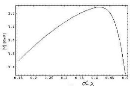
Figure 5: Typical dependence of the smallest gluonium mass (in GeV) on the coupling constant $\alpha$ between 0.15 and 0.5.

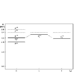
Figure 6: Gluonium masses: dashed lines are taken from lattice calculations [25]. Bold lines are obtained from $H_{\lambda}$. The mass of the state labeled $0^{++}$ was fitted to the lattice result of 1.73 GeV. The parameters in $H_{\lambda}$ are $\lambda=1.92$ GeV, $b=2\lambda$, $\delta=0.2$, $\alpha_{s}=0.44$.

slightly denser than on the lattice but otherwise it appears to be qualitatively similar. However, there is so far no clear way for associating the eigenstates with spin quantum numbers. There is no clear degeneracy into multiplets corresponding to rotational symmetry. Although the lowest masses are not widely different, and one may think that the violation of the multiplet structure is not significant given the crude nature of the calculation (cf. [23]), the question of how to improve rotational symmetry is not answered. But it is certain that a simple mass gap ansatz of Eq. (13) has no a priori reason to produce true degeneracy of the masses.

Regarding the stability of the results versus changes of $\lambda$ one can say that when $\alpha_{\lambda}$ is forced to vary with $\lambda$ according to the perturbative formula with no quarks, the results are not varying significantly with $\lambda$. But one can change the relative order of masses of $|j_{z}|=0,1,2$ eigenstates by making about 10% changes of the values of $\lambda$, $\alpha$, $b$ and $\delta$. The overall conclusion is that the gluonium picture in the boost-invariant LF Hamiltonian approach appears surprisingly reasonable even in the crude first approximation. Readers interested in more details should consult Ref. [20].

4 QUARKONIUM

Theoretical aspects of the heavy quarkonium picture emerging from LF Hamiltonians for QCD with one heavy flavor and gluon mass gap ansatz are described in Ref. [1] and do not need to be repeated here. The main feature is that all details of the mass ansatz for effective gluons in the sector $|Q_{\lambda}\bar{Q}_{\lambda}g_{\lambda}\rangle$ disappear from the effective Hamiltonian in the $|Q_{\lambda}\bar{Q}_{\lambda}\rangle$ sector and the resulting second-order eigenvalue problem turns out to be exactly rotationally invariant. The first correction to the Coulomb potential is a force resembling a harmonic oscillator.

The fact that a mass gap ansatz leads to an oscillator-like interaction term which respects rotational symmetry already in the 2nd order analysis using $\mu^{2}\sim 1$ does not seem accidental. This result appears almost independently of all details of the ansatz because momentum transfer squared, $q^{2}$, in the terms that are sensitive to small-$x$ of the gluons, is limited by the RGPEP form factors $f_{\lambda}$ to so small values that the ratio $\mu^{2}/(q^{2}+\mu^{2})$ is practically 1 for any reasonable ansatz. In addition, it seems likely that the same result comes out also as a part of the genuine 4th order calculation (not completed yet). In the 4th order, the ansatz term $\mu^{2}\sim 1$ cancels out for large physical $\alpha$ [1]. The next term comes from QCD interactions order $\alpha$ in the 3-body sector and this is how the actual gap may show up. But $q^{2}$ in a system dominated by the Coulomb force (the case of quark masses very much larger than $\Lambda_{QCD}$) continues to be formally on the order of the strong Bohr momentum squared, or order $\alpha^{2}$ which is much smaller than $\mu^{2}$ when $\mu^{2}\sim\alpha$. If this observation is confirmed in 4th order calculations, the spherical symmetry of the leading oscillator term identified already in the 2nd order using the ansatz for $\mu^{2}$, may be a necessary consequence of the rotational symmetry of QCD.

One should observe two general arguments that support the harmonic result in the first approximation. One argument is that the combined effect of the self-interactions and the exchange leads to binding above threshold which emerges around a minimum of the mass squared operator derived from the LF Hamiltonian $P^{-}$ and every function around a minimum is in the first approximation a quadratic one. The question is not so much why the potential comes out quadratic but rather what the spring (not string) constant is. Quite general Coulomb scaling argument implies that the spring constant is on the order of $k\sim\alpha\lambda^{6}/m^{3}$. But if one assumes that $\lambda\sim\sqrt{\alpha}m$, the resulting harmonic potential scales with $\alpha$ exactly as the Coulomb eigenvalue problem does. This means that such harmonic force may always be of a fixed relative magnitude to the Coulomb part of the interaction if QCD develops a mass gap for the effective gluons. The other argument is that when the distance between the heavy quarks increases, a linear potential may develop between the quarks at the expense of creating additional gluons with a mass gap if the potential grows faster than linearly [26, 27] - it becomes energetically more favorable to create a definite number of gluons per unit of length than to allow the potential energy to grow without creating additional gluons. And the first possible integer power of the distance is 2. Thus, the harmonic force is probably the simplest one that can lead to a string picture in LF Hamiltonians for QCD.

The simplicity of the LF Hamiltonian approach can now be exhibited using a calculation performed by a freshman on a personal computer [28]. When one neglects all spin effects and then disregards parameters that play no role in the spinless case, the eigenvalue equation for heavy quarkonia that one derives from the LF Hamiltonian reads

$$\left[-\frac{\Delta_{r}}{2m}\,-\,\frac{4\alpha}{3r}+\frac{k}{2}\,r^{2}\right]\,\Psi(\vec{r})\,=\,E\,\Psi(\vec{r})\,,$$ (14)

where $m$ is the reduced quark mass, equal half of the quark mass $m_{q}$. The eigenvalue $E$ gives the quarkonium mass through the formula

$$M=2m_{q}\sqrt{1+E/m_{q}}\,,$$ (15)

which is relativistic.

Stawikowski found that for $k$ = 0.0431 GeV³, $2m=m_{b}$ = 5.0006 GeV, $\alpha$ = 0.6029, all compatible with the range of parameters a priori possible in LF QCD, the masses of $\Upsilon$ states $1S$, $2S$, and $3S$, could be reproduced with precision of $10^{-5}$, or $\pm 0.05$ MeV. Such accuracy is understandable because one has three parameters to fit three masses (Stawikowski considered a Coulomb potential multiplied by the factor $e^{-\mu r}(1-e^{\lambda r})$ but for the values $\mu=10^{-6}$ GeV and $\lambda=4$ GeV that he used, these additional parameters were not important). The same parameters give $M_{1P}$ = 9.9144 GeV (the experimental average of masses of $1P$ bottomonium states is 9.8884 GeV), and $M_{2P}$ = 10.2507 GeV (the experimental average of masses of $2P$ bottomonium states is 10.2519 GeV).

Keeping the same parameters $k$ and $\alpha$ and changing the quark mass to $m_{c}=1.6068$ GeV, one obtains the experimental value of the mass of $J/\Psi$ state, $M_{1S}$ = 3.0969 GeV. The $2S$ state obtains the mass $M_{2S}$ = 3.6628 GeV (the experimental value is 3.6861 GeV), and the state $1P$ obtains $M_{1P}$ = 3.4991 GeV (the experimental average of masses of $1P$ charmonium states is 3.4940 GeV). It is clear that the harmonic oscillator potential as an admixture to the Coulomb potential is a qualitatively acceptable one from the point of view of such fit. An extensive numerical study including spin effects is under way [29].

5 CONCLUSION

The second-order RGPEP procedure for deriving LF Hamiltonians for heavy quarks and gluons produces operators that seem to have a chance of providing a qualitatively reasonable first approximation of the dynamical picture for masses of gluonium and quarkonia. Rotational symmetry requires intensive studies, especially in the case of gluonium (important gluon degrees of freedom appear also in hybrids and there one faces considerable constraints due to rotational symmetry [30]). The picture of binding mechanism that one can hold on to in order to build further intuitions is based on the possibility to control behavior of self-interactions of quarks and gluons in the effective Hamiltonians with small RGPEP parameter $\lambda$. The self-interactions largely reduce positive contributions from counterterms, but not entirely, and the exchange of gluons can lead to bound-state masses above threshold. The RGPEP procedure can be applied to many more cases than only those discussed here and one can refine the picture using higher order perturbation theory and a whole arsenal of methods for solving quantum Hamiltonian problems. An extension of the approach to include light quarks will be more complicated than the heavy quarkonium case. But the example of gluonium suggests that the required fourth order RGPEP studies may shed new light on the issue of how to approach eigenvalue problems including light quarks. So far, no vacuum structure was involved in the entire calculation.

The rotationally symmetric effective Hamiltonians described here provide an interesting addition to earlier studies based on similarity renormalization group and coupling coherence [31, 32, 33, 34, 35]. But it is not clear yet if the RGPEP procedure for LF Hamiltonians will ever match the accuracy of methods applicable in QED [36, 37] or in lattice-based calculations [38, 39]. One has to be aware that a constituent picture can be fitted to data using a large range of potentials [40, 41]. On the other hand, if the hypothesis that QCD has an infrared limit cycle [42, 43] is correct, it may turn out that new Hamiltonian methods provide a path to understanding of the limit cycle universality [44] required for systematic solution of the theory.

It is my pleasure to acknowledge discussions with Tomasz Masłowski, Jarosław Młynik, Jakub Narȩbski, Lech Stawikowski, and Marek Wiȩckowski. I thank Kenneth G. Wilson for numerous discussions on the renormalization of Hamiltonians at the early stages of the development of the theory. I would like to thank the Organizers for a very interesting Workshop.

References

- [1] S. D. Głazek, Phys. Rev. D69, 065002 (2004).
- [2] M. Gell-Mann, in Proceedings of the Eleventh International Universitätswochen für Kernphysik, Schladming, Austria, edited by P. Urban (Springer, New York, 1972), p. 733.
- [3] H. Fritsch and M. Gell-Mann, in Proceedings of the XVI International Conference on High Energy Physics, Chicago-Batavia, Ill., 1972, edited by J. D. Jackson and A. Roberts (NAL, Batavia, Ill., 1973), Vol. 2, p. 135.
- [4] H. J. Melosh, Phys. Rev. D9, 1095 (1974).
- [5] S. D. Głazek, Acta Phys. Pol. B29, 1979 (1998).
- [6] P. A. M. Dirac, Rev. Mod. Phys. 21, 392 (1949).
- [7] S. D. Głazek, T. Masłowski, Phys. Rev. D65, 065011 (2002).
- [8] M. Wiȩckowski, Ph.D. Thesis, Warsaw Univ. 2005; see also hep-th/0511148.
- [9] C. B. Thorn, Nucl. Phys. B699, 427 (2004); hep-th/0405018.
- [10] C. B. Thorn, hep-th/0507213.
- [11] S. D. Głazek, K. G. Wilson, Phys. Rev. D48, 5863 (1993).
- [12] S. D. Głazek, K. G. Wilson, Phys. Rev. D49, 4214 (1994).
- [13] S. D. Głazek, J. Młynik, Acta Phys. Polon. B35, 723 (2004).
- [14] F. J. Wegner, Ann. Phys. (Leipzig) 3, 77 (1994).
- [15] F. J. Wegner, Phys. Rep. 348, 77 (2001).
- [16] S. D. Głazek, J. Młynik, Phys. Rev. D67, 045001 (2003).
- [17] S. D. Głazek, M. Wiȩckowski, Phys. Rev. D66, 016001 (2002).
- [18] B. D. Jones, R. J. Perry, S. D. Głazek, Phys. Rev. D55, 6561 (1997).
- [19] K. G. Wilson, Phys. Rev. D 2, 1438 (1970).
- [20] T. Masłowski, Ph.D. Thesis, Warsaw Univ. 2005; maslo@fuw.edu.pl.
- [21] K. G. Wilson et al. Phys. Rev. D49, 6720 (1994).
- [22] G. P. Lepage, S. J. Brodsky, Phys. Rev. D22, 2157 (1980).
- [23] B. H. Allen, R. J. Perry, Phys. Rev. D62, 025005 (2000).
- [24] G. ’t Hooft, Nucl. Phys. B75, 461 (1974).
- [25] C. J. Morningstar, M. J. Peardon, Phys. Rev. D60, 034509 (1999).
- [26] K. G. Wilson Phys. Rev. Lett. 27, 690 (1971).
- [27] J. Kogut and L. Susskind, Phys. Rev. D9, 697 (1974).
- [28] L. Stawikowski, in preparation.
- [29] S. D. Głazek, J. Młynik, in preparation.
- [30] S. D. Głazek, J. Narȩbski, hep-ph/0510398.
- [31] R. J. Perry and K. G. Wilson, Nucl. Phys. B403, 587 (1993).
- [32] R. J. Perry, Ann. Phys. 232, 116 (1994).
- [33] R. J. Perry, in Proc. of Hadrons 94, eds. V. Herscovitz and C. Vasconcellos (World Scientific, 1995); hep-th/9407056.
- [34] M. Brisudová and R. Perry, Phys. Rev. D54, 1831 (1996).
- [35] M. M. Brisudová, R. J. Perry and K. G. Wilson, Phys. Rev. Lett. 78, 1227 (1997).
- [36] W. E. Caswell and G. P. Lepage, Phys. Lett. B167, 437 (1986).
- [37] K. Pachucki, Phys. Rev. A56, 297 (1997).
- [38] B. A. Thacker, G. P. Lepage, Phys. Rev. D43, 196-208 (1991).
- [39] G. T. Bodwin, E. Braaten, and G. P. Lepage, Phys. Rev. D51, 1125 (1995); 55, 5853(E) (1997).
- [40] L. Motyka, K. Zalewski, Z. f. Physik C69, 343 (1996).
- [41] K. Zalewski, Acta Phys. Polon. B29, 2535 (1998).
- [42] E. Braaten and H. W. Hammer, Phys. Rev. Lett. 91, 102002 (2003).
- [43] K. G. Wilson, Nucl. Phys. Proc. Suppl. 140,3 (2005); hep-lat/0412043.
- [44] S. D. Głazek and K. G. Wilson, Phys. Rev. B69, 094304 (2004).