High-accuracy critical exponents of $O(N)$ hierarchical sigma models

Abstract

We perform high-accuracy calculations of the critical exponent $\gamma$ and its subleading exponent for the $3D$ $O(N)$ Dyson’s hierarchical model for $N$ up to 20. We calculate the critical temperatures for the nonlinear sigma model measure $\delta(\vec{\phi}.\vec{\phi}-1)$. We discuss the possibility of extracting the first coefficients of the $1/N$ expansion from our numerical data. We show that the leading and subleading exponents agree with Polchinski equation and the equivalent Litim equation, in the local potential approximation, with at least 4 significant digits.

The large $N$ limit and the $1/N$ expansion Stanley (1968); Ma (1973); ’t Hooft (1974a) appear prominently in recent developments in particle physics, condensed matter and string theory Teper (2005); Narayanan and Neuberger (2005); Moshe and Zinn-Justin (2003); Aharony et al. (2000). For sigma models, the basic gap equation can be obtained by using the method of steepest descent for the functional integral Stanley (1968); David et al. (1985). For $N$ large and negative, the maxima of the action dominate instead of the minima and the radius of convergence of the $1/N$ expansion should be zero. In order to turn a $1/N$ expansion into a quantitative tool, we need to: 1) understand the large order behavior of the series, 2) locate the singularities of the Borel transform and, 3) compare the accuracy of various procedures with numerical results for given values of $N$. Calculating the series or obtaining accurate numerical results at fixed $N$ are difficult tasks and we do not know any model where this program has been completed. For instance for the critical exponents in three dimensions, we are only aware of calculation up to order $1/N^{2}$ in Ref. Okabe et al. (1978); Gracey (1991); Pelissetto and Vicari (2002). Several results related to the possibility (or impossibility) of resumming particular $1/N$ expansions are known de Wit and ’t Hooft (1977); Avan and de Vega (1984); Kneur and Reynaud (2003). Overall, it seems that there is a rather pessimistic impression regarding the possibility of using the $1/N$ expansion for low values of $N$. For this reason, it would be interesting to discuss the three questions enumerated above for a model where we have good chances to obtain definite answers. Dyson’s hierarchical model Dyson (1969); Baker (1972) is a good candidate for this purpose.

In this Brief Report, we provide high-accuracy numerical values for the critical exponent $\gamma$, the subleading exponent $\Delta$ and the critical parameter $\beta_{c}$ for the $3D$ $O(N)$ hierarchical nonlinear sigma models. These quantities appear in the magnetic susceptibility near $\beta_{c}$ in the symmetric phase as

$$\chi=(\beta_{c}-\beta)^{-\gamma}(A_{0}+A_{1}(\beta_{c}-\beta)^{\Delta}+\dots)\ .$$ (1)

The method of calculation of the critical exponents used here is an extension of one of the methods described at length in the case of $N=1$ Godina et al. (1999) and will only be sketched briefly. On the other hand, the accuracy of the approximations used depend non trivially on $N$ as we shall discuss later. The RG transformation can be constructed as a blockspin transformation followed by a rescaling of the field. For Dyson’s hierarchical model, the block spin transformation affects only the local measure. The RG transformation can be expressed conveniently in terms of the Fourier transform (denoted $R$ hereafter) of this local measure. In the following, we keep the $O(N)$ symmetry unbroken and the Fourier transform will depend only on $\vec{k}.\vec{k}\equiv u$. Here $\vec{k}$ is a source conjugated to the local field variable $\vec{\phi}$. Replacing $k$ by $u$ and the second derivative by the $N$-dimensional Laplacian in Eq. (2.5) of Ref. Godina et al. (1999), we obtain the RG transformation for the Fourier transform of the local measure:

$$R_{n+1,N}(u)\propto{\rm e}^{\left[-\frac{1}{2}\beta\left(4u\frac{\partial^{2}}{\partial u^{2}}+2N\frac{\partial}{\partial u}\right)\right]}\left(R_{n,N}\left(cu/4\right)\right)^{2}\ ,$$ (2)

where $c=2^{1-2/D}$ in order to reproduce the scaling of a Gaussian massless field in $D$ dimensions. $D=3$ hereafter. We fix the normalization constant by imposing $R_{n,N}(0)=1$ so that $R_{n,N}(k)$ has a simple probabilistic interpretation Godina et al. (1999). In the following, the calculations will be performed using polynomial approximations of degree $l_{\max}$:

$$R_{n,N}(k)\simeq 1+a_{n,1}u+a_{n,2}u^{2}+\cdots+a_{n,l_{\max}}u^{l_{\max}}\ .$$ (3)

The finite volume susceptibility for $2^{n}$ sites is related to the first coefficient by the relation $\chi_{n}=-2a_{n,1}(2/c)^{n}$. The truncated recursion formula for the $a_{n,m}$ reads

$$a_{n+1,m}=\frac{\sum_{l=m}^{2l_{\max}}\left(\sum_{p+q=l}a_{n,p}a_{n,q}\right)B_{m,l}}{\sum_{l=0}^{2l_{\max}}\left(\sum_{p+q=l}a_{n,p}a_{n,q}\right)B_{0,l}}\ ,$$ (4)

with

$$B_{m,l}=\frac{\Gamma(l+1)\Gamma(l+N/2)}{\Gamma(m+1)\Gamma(m+N/2)}\frac{1}{(l-m)!}(\frac{c}{4})^{l}(-2\beta)^{l-m}\ .$$ (5)

We emphasize that in the above formula and in our numerical calculations, no truncation is applied after squaring and so the sum in Eq. (4) does extend up to $2l_{max}$. Since the derivatives appear to arbitrarily large order in Eq. (2) and can lower the degree of a polynomial of order larger than $l_{max}$, this affects all the coefficients of order less than $l_{max}$. This procedure has been discussed and justified in Ref. Meurice and Niermann (2002).

The critical exponents appearing in Eq. (1) are obtained by calculating the eigenvalues $\lambda_{1},\lambda_{2},\dots$ of the matrix $\partial a_{n+1,l}/\partial a_{n,m}$ at the nontrivial fixed point. The exponents $\gamma$ and $\Delta$, can be expressed as

$$\gamma=\frac{\ln(2/c)}{\ln(\lambda_{1})}{\rm\ \ ,\ \ }\Delta=\left|\frac{\ln(\lambda_{2})}{\ln(\lambda_{1})}\right|\ .$$ (6)

The critical exponents are universal and, within numerical errors, independent of the manner that we approach the nontrivial fixed point. In the following, we have mostly started with the local measure of the nonlinear sigma model $\delta(\vec{\phi}.\vec{\phi}-1)$. The corresponding Fourier transform reads

$$R_{0,N}(u)=\sum_{l=0}^{\infty}\frac{(-1)^{l}u^{l}\Gamma(\frac{N}{2})}{2^{2l}l!\Gamma(\frac{N}{2}+l)}\ .$$ (7)

A motivation for this choice is that, as we will explain below, the value of $\beta_{c}$ can be calculated in the large $N$ limit. Other measures have also been used in order to check the universal values of the two exponents.

The asymptotic behavior of the ratio $a_{n+1,1}/a_{n,1}$ allows us to decide unambiguously if we are in the symmetric phase (where the ratio approaches $c/2\simeq 0.63$) or in the broken phase (where the ratio approaches $c$). Using a binary search, one can determine the critical value of $\beta$ with great accuracy. As this critical value depends on $l_{max}$, we denote it $\beta_{c}(l_{max})$. When $l_{max}\rightarrow\infty$, $\beta_{c}(l_{max})\rightarrow\beta_{c}$. The rate at which this limit is reached depends on $N$. This is illustrated in Fig. 1 where we see that in order to reach $\beta_{c}$ with a given accuracy, we need to increase $l_{max}$ when $N$ increases. In Fig. 2, we give the minimum $l_{max}$ necessary for $\beta_{c}(l_{max})$ to share 20 significant digits with $\beta_{c}$. $l_{max}\simeq 22+6.2N^{0.7}$ is a good fit for Fig. 2.

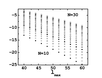
Figure 1: $\log_{10}\frac{|\beta(l_{\max})-\beta_{c}|}{\beta_{c}}$ calculated for $l_{\max}=40$ to $l_{\max}=60$ for $N=10$ (filled circles), $N=11$ (empty circles), $N=12$ (empty triangles) …… up to $N=30$ (empty squares).

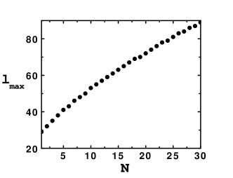
Figure 2: Minimal value of $l_{\max}$ in order to have $\log_{10}\frac{|\beta_{c}(l_{\max})-\beta_{c}(\infty))|}{\beta_{c}(\infty)}=-20$ versus $N$.

The nontrivial fixed point for a given value of $l_{max}$ can be constructed by iterating sufficiently many times the RG map at values sufficiently close to $\beta_{c}(l_{\max})$. In order to get an accuracy $\epsilon$ for the fixed point for that value of $l_{max}$, we need to iterate $n$ times the map until

$$\lambda_{2}^{n}\sim\epsilon\ ,$$ (8)

in order to get rid of the irrelevant directions. At the same time, we want the growth in the relevant direction to be limited, in other words,

$$|\beta-\beta_{c}(l_{\max})|\lambda_{1}^{n}<\epsilon\ .$$ (9)

Combining these two requirements together with Eq. (6) we obtain

$$|\beta-\beta_{c}(l_{\max})|\simeq\epsilon^{1+1/\Delta}$$ (10)

This is an order magnitude estimate, however it works well except for $N$=1 where we need to pick $\beta$ slightly closer to the critical value. By “working well”, we mean that if we go closer to the critical value, changes smaller than $\epsilon$ are observed in the first two eigenvalues. The numerical results for $\epsilon=10^{-10}$ and $N$ up to 20, are given in the Tables 1 and 2 for the values of $l_{max}$ of Fig. 2. Errors of 1 or less in the last printed digit should be understood in all the tables.

Table 1: $\beta_{c}$ and the first two eigenvalues for $N=1\dots 20$.

$N$	$\beta_{c}$	$\lambda_{1}$	$\lambda_{2}$
1	1.1790301704462697325	1.427172478	0.8594116492
2	2.4735265752919854000	1.385743490	0.8563409066
3	3.8273820333573397671	1.354668326	0.8506945150
4	5.2111615635533656165	1.332749866	0.8440522956
5	6.6104153462855068435	1.317578283	0.8376436747
6	8.0181114053706725941	1.306955396	0.8320345022
7	9.4307096447427796882	1.299321025	0.8273378172
8	10.846330737925124699	1.293666393	0.8234676785
9	12.263918029354988652	1.289354227	0.8202833449
10	13.682844072802585664	1.285978489	0.8176485461
11	15.102717572108367579	1.283274741	0.8154492652
12	16.523283812777939366	1.281066141	0.8135953137
13	17.944370719047342283	1.279231192	0.8120168555
14	19.365858255947423937	1.277684252	0.8106600963
15	20.787660334686062513	1.276363511	0.8094834857
16	22.209713705054412233	1.275223389	0.8084547150
17	23.631970906283518487	1.274229622	0.8075484440
18	25.054395659078177206	1.273356000	0.8067446107
19	26.476959772907788848	1.272582158	0.8060271793
20	27.899641020779716433	1.271892050	0.8053832116

Table 2: $\gamma$, $\Delta$ and $\beta_{c}/N$ for $N=1\dots 20$.

$N$	$\gamma$	$\Delta$	$\beta_{c}/N$
1	1.29914073	0.425946859	1.179030170
2	1.41644996	0.475380831	1.236763288
3	1.52227970	0.532691965	1.275794011
4	1.60872817	0.590232008	1.302790391
5	1.67551051	0.642369187	1.322083069
6	1.72617703	0.686892637	1.336351901
7	1.76479863	0.723880426	1.347244235
8	1.79469274	0.754352622	1.355791342
9	1.81827105	0.779508505	1.362657559
10	1.83722291	0.800424484	1.368284407
11	1.85272636	0.817977695	1.372974325
12	1.86561092	0.832855522	1.376940318
13	1.87646998	0.845589221	1.380336209
14	1.88573562	0.856588705	1.383275590
15	1.89372812	0.866171682	1.385844022
16	1.90068903	0.874586271	1.388107107
17	1.90680338	0.882027998	1.390115936
18	1.91221507	0.888652409	1.391910870
19	1.91703752	0.894584429	1.393524199
20	1.92136121	0.899925325	1.394982051
$\infty$	2	1	$\frac{2-c}{2(c-1)}=1.42366..$

As $N$ increases, the values displayed in Table 2 seem to slowly approach asymptotic values. This is expected. Using the general formulation of Ref. Ma (1973); David et al. (1985) together with the particular form of the propagator Meurice (2003) for the model considered here, one finds the leading terms

$$\gamma \simeq 2+a_{1}/N+\dots$$ (11)

$$\Delta \simeq 1+b_{1}/N+\dots$$

$$\beta_{c}/N \simeq (2-c)/(2(c-1))+c_{1}/N+\dots\ .$$ (12)

The magnitude of the coefficients $a_{1},\ b_{1},\ c_{1}$ of the leading $1/N$ corrections can be estimated by subtracting the asymptotic value and multiplying by $N$. The results are shown in Table 3. They indicate that $a_{1}\simeq-1.6,\ b_{1}\simeq-2.0,\ c_{1}\simeq-0.57$. It seems possible to improve the accuracy by estimating the next to leading order corrections and so on. However, the stability of this procedure is more delicate and remains to be studied with simpler examples.

Table 3: $N(2-\gamma)$, $N(1-\Delta)$ and $N(\frac{2-c}{2(c-1)}-\frac{\beta_{c}}{N})$ for $N=1\dots 20$..

$N$	$N(2-\gamma)$	$N(1-\Delta)$	$N(\frac{2-c}{2(c-1)}-\frac{\beta_{c}}{N})$
1	0.7009	0.5741	0.2446
2	1.167	1.049	0.3738
3	1.433	1.402	0.4436
4	1.565	1.639	0.4835
5	1.622	1.788	0.5079
6	1.643	1.879	0.5239
7	1.646	1.933	0.5349
8	1.642	1.965	0.5430
9	1.636	1.984	0.5490
10	1.628	1.996	0.5538
11	1.620	2.002	0.5576
12	1.613	2.006	0.5606
13	1.606	2.007	0.5632
14	1.600	2.008	0.5654
15	1.594	2.007	0.5673
16	1.589	2.007	0.5689
17	1.584	2.006	0.5703
18	1.580	2.004	0.5715
19	1.576	2.003	0.5726
20	1.573	2.001	0.5736

We now compare the exponents calculated here with those calculated with three other RG transformations Comellas and Travesset (1997); Gottker-Schnetmann (1999); Litim (2002). As we proceed to explain, the exponents should be the same in the four cases (including ours). The change of coordinates that relates the RG transformation considered here and the one studied in Ref. Gottker-Schnetmann (1999) is given in the introduction of Koch and Wittwer (1991) (for $L=2^{1/3}$). The fact that the limit $L\rightarrow 1$ in the formulation of Ref. Gottker-Schnetmann (1999) yields the Polchinski equation in the local potential approximation studied in Ref. Comellas and Travesset (1997) is explained in Ref. Felder (1987). Consequently, these two RG transformations should be the same in the linear approximation. Finally, Litim Litim (2000, 2002) proposed an optimized version of the exact RG transformation and suggested Litim (2005) that it was equivalent to the Polchinski equation in the local potential approximation. The equivalence was subsequently proved by Morris Morris (2005).

To facilitate the comparison, we display $\nu=\gamma/2$ (since $\eta=0$ here) and $\omega=\Delta/\nu$ in Table 4. Our results coincide with the 4 digits given in column (2) of Table 3 (for $\nu$) and 4 (for $\omega$) in Comellas and Travesset (1997). They coincide with the six digits for $\nu$ given in the line $d=3$ of Table 8 of Gottker-Schnetmann (1999) for $N$= 1, 2, 3, 5 and 10. However, we found discrepancies of order 1 in the fifth digit of $\nu$ and slightly larger for $\omega$ with the values found in Table 1 of Litim (2002). Our estimated errors are of order 1 in the 9-th digit. For $N=1$, this is confirmed by an independent method Godina et al. (1999). For $N=$ 2, 3, 5, and 10, this is confirmed up to the sixth digit Gottker-Schnetmann (1999). Consequently, a discrepancy in the 5-th digit cannot be explained by our numerical errors. Note also that for $N\geq 2$, $\alpha$ is more negative than for nearest neighbor models Pelissetto and Vicari (2002).

In summary, we have provided high-accuracy data for $\gamma$, $\Delta$ and $\beta_{c}$ for $N$ up to 20. It seems likely that a few terms of the $1/N$ expansion for these three quantities can be estimated from this data. Work is in progress to calculate these expansions independently by semi-analytical methods and learn about the asymptotic behavior of the series and their accuracy. The discrepancy with the 5-th digit of Ref. Litim (2002) remains to be explained.

We thank G. ’t Hooft, J. Zinn-Justin and G. Parisi for valuable comments on related topics. This research was supported in part by the Department of Energy under Contract No. FG02-91ER40664. M.B. Oktay has been supported by SFI grant 04/BRG/P0275.

Table 4: $\nu$, $\omega$ and $\alpha$ for $N=1\dots 20$.

$N$	$\nu=\gamma/2$	$\omega=\Delta/\nu$	$\alpha=2-3\nu$
1	0.649570	0.655736	0.051289
2	0.708225	0.671229	-0.124675
3	0.761140	0.699861	-0.283420
4	0.804364	0.733787	-0.413092
5	0.837755	0.766774	-0.513266
6	0.863089	0.795854	-0.589266
7	0.882399	0.820355	-0.647198
8	0.897346	0.840648	-0.692039
9	0.909136	0.857417	-0.727407
10	0.918611	0.871342	-0.755834

References

- Stanley (1968) H. E. Stanley, Phys. Rev. 176, 718 (1968).
- Ma (1973) S. K. Ma, Phys. Lett. A43, 475 (1973).
- ’t Hooft (1974a) G. ’t Hooft, Nucl. Phys. B72, 461 (1974a); Nucl. Phys. B75, 461 (1974b).
- Moshe and Zinn-Justin (2003) M. Moshe and J. Zinn-Justin, Phys. Rept. 385, 69 (2003), eprint hep-th/0306133.
- Aharony et al. (2000) O. Aharony, S. S. Gubser, J. M. Maldacena, H. Ooguri, and Y. Oz, Phys. Rept. 323, 183 (2000), eprint hep-th/9905111;
- Narayanan and Neuberger (2005) R. Narayanan and H. Neuberger (2005), eprint hep-lat/0501031.
- Teper (2005) M. Teper (2005), eprint hep-lat/0509019.
- David et al. (1985) F. David, D. A. Kessler, and H. Neuberger, Nucl. Phys. B257, 695 (1985).
- Okabe et al. (1978) Y. Okabe, M. Oku, and R. Abe, Prog. Theor. Phys. 59, 1825 (1978).
- Gracey (1991) J. A. Gracey, J. Phys. A24, L197 (1991).
- Pelissetto and Vicari (2002) A. Pelissetto and E. Vicari, Phys. Rept. 368, 549 (2002), eprint cond-mat/0012164.
- de Wit and ’t Hooft (1977) B. de Wit and G. ’t Hooft, Phys. Lett. B69, 61 (1977).
- Avan and de Vega (1984) J. Avan and H. J. de Vega, Phys. Rev. D29, 2904 (1984).
- Kneur and Reynaud (2003) J. L. Kneur and D. Reynaud, JHEP 01, 014 (2003), eprint hep-th/0111120.
- Dyson (1969) F. Dyson, Comm. Math. Phys. 12, 91 (1969).
- Baker (1972) G. Baker, Phys. Rev. B5, 2622 (1972).
- Godina et al. (1999) J. Godina, Y. Meurice, and M. Oktay, Phys. Rev. D 59, 096002 (1999).
- Meurice and Niermann (2002) Y. Meurice and S. Niermann, J. Statist. Phys. 108, 213 (2002), eprint cond-mat/0105380.
- Meurice (2003) Y. Meurice, Phys. Rev. D67, 025006 (2003), eprint hep-th/0208181.
- Litim (2002) D. F. Litim, Nucl. Phys. B631, 128 (2002), eprint hep-th/0203006.
- Comellas and Travesset (1997) J. Comellas and A. Travesset, Nucl. Phys. B498, 539 (1997), eprint hep-th/9701028.
- Gottker-Schnetmann (1999) J. Gottker-Schnetmann (1999), eprint cond-mat/9909418 (unpublished).
- Koch and Wittwer (1991) H. Koch and P. Wittwer, Commun. Math. Phys. 138, 537 (1991).
- Felder (1987) G. Felder, Commun. Math. Phys. 111, 101 (1987).
- Litim (2000) D. F. Litim, Phys. Lett. B486, 92 (2000), eprint hep-th/0005245.
- Litim (2005) D. F. Litim, JHEP 07, 005 (2005), eprint hep-th/0503096.
- Morris (2005) T. R. Morris, JHEP 07, 027 (2005), eprint hep-th/0503161.