Observational constraints on braneworld geometry

Abstract

The low energy regime of 5D braneworld models with a bulk scalar field is studied. The setup is rather general and includes the Randall-Sundrum and dilatonic braneworlds models as particular cases. We discuss the cosmological evolution of the system and conclude that, in a two brane system, the negative tension brane is generally expected to evolve towards a null warp-factor state. This implies, for late time cosmology, that both branes end up interacting weakly. We also analyze the observational constraints imposed by solar-system and binary-pulsar tests on the braneworld configuration. This is done by considering the small deviations produced by the branes on the 4D gravitational interaction between bodies in the same brane. Using these constraints we show that the geometry around the braneworld is strongly warped, and that both branes must be far apart.

I Introduction

Braneworld models have been shown to be extremely rich in phenomena leading to modifications of General Relativity (GR) at both low and high energies Langlois ; Maartens ; brax-bruck-davis . When the four-dimensional description of branes is considered, massless scalar degrees of freedom -the moduli- appear mediating the gravitational interaction together with the usual 4D graviton. The presence of these moduli is commonly related to the geometry of the entire system and plays a significant role in the phenomenology of extra-dimensions. At low energies, for instance, braneworld models are best described by scalar-tensor theories scalar-tensor1 ; scalar-tensor2 ; scalar-tensor3 ; scalar-tensor4 ; scalar-tensor5 ; Kanti1 ; Kanti2 ; Palma-Davis1 ; Palma-Davis2 . Within this framework, the gravitational couplings become functions of the moduli and standard GR predictions get modified in ways that can be tightly constrained by present astrophysical observations.

Current tests on gravity allow us to measure relativistic corrections to Newton’s law at the first post-Newtonian level ($\propto 1/c^{2}$) with great precision Edd . At this order, the predictions of scalar-tensor theories can be parameterized by two “weak field” quantities, $\beta$ and $\gamma$, the post-Newtonian parameters introduced long ago by Eddington Eddington . When solar-system tests are taken into account these parameters are observed to be very close to 1 (GR corresponds to $\beta=\gamma=1$). For example, the time delay variation of the Cassini spacecraft near the solar conjunction Cassini has given the result $\gamma-1=(2.1\pm 2.3)\times 10^{-5}$, whereas the lunar laser ranging experiment Lunar shows that $4\beta-\gamma-3=(-0.7\pm 1)\times 10^{-3}$. Another source of constraints on $\beta$ and $\gamma$, qualitatively different from solar-system tests, comes from the observation on binary pulsars systems Pulsar1 ; Pulsar2 . In this case, the “strong field” conditions generated by the compactness of neutron stars allow the analysis of nonperturbative effects caused by the moduli, implying tight bounds on the Eddington parameters.

In this paper the low energy regime of braneworld models is considered. We show that solar-system and binary-pulsar tests can be used to discriminate between different 5D braneworld models and to shed light on their extra-dimensional configuration. For this, we have chosen a rather general setup, BPS-braneworlds, of which the Randall-Sundrum model RS1 ; RS2 and dilatonic braneworlds Lukas are just particular examples. The model consists of a 5D space-time bounded by two 3-branes with tensions $\lambda_{1}$ and $\lambda_{2}$. A scalar field $\phi$ lives in the 5D bulk and is dominated by a bulk potential $U(\phi)$. At the same time, the brane tensions are functions of the scalar field boundary values, $\phi^{1}$ and $\phi^{2}$, of the form: $\lambda_{1}=+\sigma(\phi^{1})$ and $\lambda_{2}=-\sigma(\phi^{2})$, where $\sigma(\phi)$ is the brane potential. In order to stay close to GR and acceptable phenomenology pheno1 ; pheno2 , a special condition (the BPS condition) exists between the scalar field potential $U(\phi)$ and the brane potential $\sigma(\phi)$:

$$U=(\partial_{\phi}\sigma)^{2}-\sigma^{2}.$$ (1)

This condition ensures supersymmetry to be preserved near the branes SUSY1 ; SUSY2 ; SUSY3 ; SUSY4 ; SUSY5 and the existence of static vacuum solutions in the absence of matter fields. Additionally, it allows the system to be described by a simple and attractive bi-scalar-tensor theory, where the moduli ($\phi^{1}$ and $\phi^{2}$) are related to the positions of the branes on the 5D background. Deviations from the BPS condition can also be included in the formalism, resulting in the presence of dark energy.

This article is organized as follows: In Sec. II we review BPS braneworlds and introduce their low energy effective description. We also discuss some relevant aspects of these models, such as its extra-dimensional geometry and the presence of singularities. In Sec. III we deduce the system’s equations of motion and analyze the cosmological evolution of the branes. There we find that the negative tension brane is generally expected to evolve towards a state where its warp factor becomes null. For late time cosmology this result implies that both branes end up interacting only weakly. In Sec. IV, the first post-Newtonian level parameters are introduced and computed for the model. It will be found that they depend on the shape of $\sigma(\phi)$ and on the positions of the branes in the background. Then we explore the way in which solar-system and binary-pulsar tests constrain the 5D configuration for this class of models. Finally, in Sec. V we provide some concluding remarks.

II BPS Braneworlds

In this section we introduce BPS-brane models in some detail and provide their low energy effective theory.

II.1 The model

Let us consider a 5D manifold $M$ with topology $M=\mathbb{R}^{4}\times S^{1}/\mathbb{Z}_{2}$, where $\mathbb{R}^{4}$ is a fixed 4D Lorentzian manifold without boundaries and $S^{1}/\mathbb{Z}_{2}$ is the orbifold constructed from the one-dimensional circle with points identified through a $Z_{2}$-symmetry. $M$ is bounded by two branes located at the fixed points of $S^{1}/\mathbb{Z}_{2}$. Let us denote the brane surfaces by $\Sigma_{1}$ and $\Sigma_{2}$ respectively and the space $M$ bounded by the branes as the bulk space. In this model there is a bulk scalar field $\phi$ with a bulk potential $U(\phi)$ and boundary values $\phi^{1}$ and $\phi^{2}$ at the branes. The brane tensions are $\lambda_{1}=+\sigma(\phi^{1})$ and $\lambda_{2}=-\sigma(\phi^{2})$ where $\sigma(\phi)$ is the brane potential (sometimes called the superpotential). Additionally, we consider the existence of matter fields $\Psi_{1}$ and $\Psi_{2}$ localized at the branes (see Fig. 1).

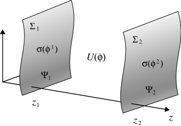
Figure 1: Schematic representation of the 5-dimensional brane configuration. In the bulk there is a scalar field $\phi$ with a bulk potential $U(\phi)$. Additionally, the bulk-space is bounded by branes, $\Sigma_{1}$ and $\Sigma_{2}$, with tensions $\lambda_{1}=+\sigma_{1}(\phi^{1})$ and $\lambda_{2}=-\sigma_{2}(\phi^{2})$ respectively.

The total action of the system is given by

$$S=S_{\mathrm{bulk}}+S_{\mathrm{branes}}+S_{\mathrm{matter}},$$ (2)

where $S_{\mathrm{bulk}}$ is the action for the bulk fields, including the gravitational field and the bulk scalar field

$$S_{\mathrm{bulk}}=\frac{1}{2\kappa_{5}^{2}}\int\!\!\sqrt{-g^{(5)}}\,d^{\,5}x\left[R^{(5)}-\frac{3}{4}\big{\{}(\partial\phi)^{2}+U\big{\}}\right].$$ (3)

Here, $g^{(5)}$ is the determinant of the five dimensional metric of signature $(-,++++)$ and $R^{(5)}$ its Ricci scalar. The term $S_{\Sigma}$ of Eq. (2) is the action for the boundary fields given by

$$S_{\mathrm{branes}}=S_{\mathrm{GH}}+S_{\phi}^{\,1}+S_{\phi}^{\,2},$$ (4)

where $S_{\mathrm{GH}}$ is the Gibbons-Hawking boundary term, and $S_{\phi}^{\,1}$ and $S_{\phi}^{\,2}$ are the brane tensions terms of the form

$$S_{\phi}^{\,1} = -\frac{3}{2\kappa_{5}^{2}}\,\int_{\Sigma_{1}}\!\!\!d^{4}x\sqrt{-g}\,\,\sigma(\phi^{1}),$$ (5)

$$S_{\phi}^{\,2} = +\frac{3}{2\kappa_{5}^{2}}\,\int_{\Sigma_{2}}\!\!\!d^{4}x\sqrt{-g}\,\,\sigma(\phi^{2}).$$ (6)

Finally, the last term in Eq. (2) corresponds to the action for the matter fields at the branes. It is given by:

$$S_{\mathrm{matter}}=S_{1}[\Psi_{1},g_{\mu\nu}^{(1)}]+S_{2}[\Psi_{2},g_{\mu\nu}^{(2)}],$$ (7)

where $\Psi_{1}$ and $\Psi_{2}$ denote the matter fields at each brane, and $g_{\mu\nu}^{(1)}$ and $g_{\mu\nu}^{(2)}$ are the respective 4D induced metrics.

To conclude, let us recall the BPS condition between the bulk potential $U$ and the superpotential $\sigma$:

$$U=\left(\partial_{\phi}\sigma\right)^{2}-\sigma^{2}.$$ (8)

Relation (8) is of the utmost importance; it allows the construction of static vacuum solutions in which the branes can be located anywhere in the background (BPS states). When $\sigma$ is a constant the Randall-Sundrum model is recovered with a negative bulk cosmological constant $\Lambda_{5}=(3/8)U=-(3/8)\,\sigma^{2}$.

Suppose that $\rho$ is the matter energy density of the braneworld universe, then, the low energy regime for this type of system is characterized by the condition $\rho\ll\sigma\kappa_{5}^{2}$. In the rest of this paper we assume that this is the case.

II.2 5D geometry

We now study the 5D geometry of the present setup. As already mentioned, in the absence of matter, condition (8) allows the construction of static vacuum solutions. This can be outlined as follows: let us assume without loss of generality that the 5D infinitesimal-metric $ds^{2}$ is given by

$$ds^{2}=N^{2}dz^{2}+g_{\mu\nu}dx^{\mu}dx^{\nu}.$$ (9)

Here, the extra-dimension is parameterized by the coordinate $z$ and $N$ is the scalar component of the 5D metric from the four-dimensional point of view (it will be related to one of the moduli on the branes). $g_{\mu\nu}$, on the other hand, is the induced 4D metric at each $z$-slice parallel to the branes (the branes are located at orbifold fixed points $z_{1}$ and $z_{2}$). Now, consider the following factorization of $g_{\mu\nu}$:

$$g_{\mu\nu}(z,x)=\omega^{2}(z)\,\tilde{g}_{\mu\nu}(x),$$ (10)

where $\tilde{g}_{\mu\nu}$ is a 4D metric satisfying the vacuum Einstein’s equation $\tilde{G}_{\mu\nu}=0$ (here $\tilde{G}_{\mu\nu}$ is the Einstein tensor constructed out of $\tilde{g}_{\mu\nu}$). Then, condition (8) allows us to find a static vacuum solution to the entire system provided that the following differential equations are fulfilled:

$$\frac{\partial\phi}{\partial z} = N\frac{\partial\sigma}{\partial\phi},$$ (11)

$$\frac{1}{\omega}\frac{\partial\omega}{\partial z} = -\frac{1}{4}N\sigma.$$ (12)

In this solution the branes can be localized anywhere in the 5D background without modifying the geometry around them. In what follows we deduce a few important results out of relations (11) and (12).

II.2.1 Parameterization of the extra-dimension

An immediate consequence of Eq. (11) is the following: if $\sigma$ is not a constant function of $\phi$ then we can parameterize the coordinate $z$ in terms of $\phi$-values:

$$Ndz=\left(\partial_{\phi}\sigma\right)^{-1}\!d\phi.$$ (13)

Note that this parameterization depends heavily on the shape of $\sigma(\phi)$. In particular, observe that as $\sigma(\phi)$ approaches a local maximum or minimum, the $z$-coordinate tends to infinity. This implies that $\partial_{\phi}\sigma$ cannot change signs in the entire bulk space. This observation simplifies much of the analysis on the braneworld geometry. Without lost of generality we may assume $\partial_{\phi}\sigma\geqslant 0$ everywhere in $M$, thus $\phi$ becomes an increasing monotonic function of $z$ (otherwise we can perform the change of variables $\phi\rightarrow-\phi$).

II.2.2 Profile of the warp factor $\omega$

Observe from Eq. (12) that the 5D geometry profile is dictated by the shape of $\sigma$; if $\sigma>0$ ($\sigma<0$) then the warp factor $\omega$ is a decreasing (increasing) function of $z$. In Sec. III we shall see that in order to have consistent dynamics at the branes, $\sigma$ must have the same sign everywhere in the bulk. In general, this implies that the brane tensions $\lambda_{1}$ and $\lambda_{2}$ must have opposite signs (as in the Randall-Sundrum model). Again, without lost of generality, we may assume that $\sigma>0$ everywhere in the bulk (otherwise, we can invert the positions of the branes). Fig. 2 shows the generic behavior for $\omega$ and $\phi$ as functions of $z$.

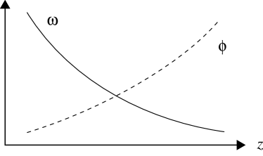
Figure 2: The figure shows the generic behavior of the warp factor $\omega$ and the scalar field $\phi$ as functions of $z$. We can always choose $\phi$ to increase and $\omega$ to decrease in the $z$-direction.

Putting Eqs. (11) and (12) together, $\omega(z)$ can be solved and expressed in terms of $\phi(z)$ in an $N$-independent way:

$$\omega(z) = \exp\left[-\frac{1}{4}\int_{\phi_{*}}^{\phi(z)}\!\!\alpha^{-1}(\phi)\,d\phi\right],$$ (14)

$$\alpha(\phi) = \frac{1}{\sigma}\frac{\partial\sigma}{\partial\phi}.$$ (15)

Here $\phi_{*}$ is an arbitrary constant value for $\phi$. If we define $\omega_{1}=\omega(z_{1})$ and $\omega_{2}=\omega(z_{2})$, then the induced metrics to the first and second branes are $\omega^{2}_{1}\,\tilde{g}_{\mu\nu}$ and $\omega^{2}_{2}\,\tilde{g}_{\mu\nu}$ respectively. Furthermore, both metrics are conformally related by the warp factor

$$\omega_{2}/\omega_{1}=\exp\left[-\frac{1}{4}\int_{\phi^{1}}^{\phi^{2}}\!\!\alpha^{-1}\,d\phi\right].$$ (16)

The parameter $\alpha$ defined in Eq. (15) will have an important role in the rest of the paper.

II.2.3 Existence of singularities

Finally, consider the possibility of having singularities at a finite position in the bulk. Singularities appear in the bulk either if $\omega(z_{1})=+\infty$ or $\omega(z_{2})=0$. Thus, Eq. (16) tells us that singularities exist provided that the following integral diverges:

$$\int_{\phi^{1}}^{\phi^{2}}\!\!\!\!\!\alpha^{-1}(\phi)\,d\phi\rightarrow+\infty.$$ (17)

Recall that $\sigma$ and $\alpha$ are positive in the entire domain $(\phi^{1},\phi^{2})$ meaning that singularities can only appear if $\alpha^{-1}=\sigma\,(\partial_{\phi}\sigma)^{-1}$ diverges at any of the two boundary values $\phi^{1}$ or $\phi^{2}$. Since the case $\partial_{\phi}\sigma=0$ corresponds to $z=\pm\infty$, we conclude that the only possible bulk-singularities are those where $\sigma(\phi^{2})=+\infty$. This corresponds to $\omega_{2}=0$. From Eq. (13) we see that for such a singularity to be located in the bulk at a finite distance from the first brane $\Sigma_{1}$, the following additional condition must hold:

$$0<\int_{\phi^{1}}^{\phi^{2}}\left(\frac{\partial\sigma}{\partial\phi}\right)^{\!\!-1}d\phi<+\infty.$$ (18)

It should be mentioned that in this analysis $\phi^{2}$ is allowed to reach arbitrary large values.

II.3 4D effective theory

We finish this section with the introduction of the low energy effective action describing the system (see Palma-Davis1 ; Palma-Davis2 for a detailed study on BPS-braneworld effective theories). For the present discussion it will be convenient to display the theory in two different (but equivalent) frames: The “background” frame, where the gravitational field $\tilde{g}_{\mu\nu}$ is the same one of Eq. (10); and the Einstein’s frame, where the term (in the action) containing the Ricci scalar is independent of the moduli $\phi^{1}$ and $\phi^{2}$. Before continuing, please notice that in the following discussion we shall use the warp factors $\omega_{1}$ and $\omega_{2}$ instead of the boundaries $\phi^{1}$ and $\phi^{2}$ to parameterize the moduli-space [the relation between these two pairs is easily obtained from Eq. (14)].

II.3.1 Background frame

In this frame, the low energy effective action for the $\omega$-fields reads:

$$S = \frac{3}{4\pi G_{*}}\int d^{4}x\sqrt{-\tilde{g}}\bigg{[}\frac{W^{2}}{12}\tilde{R}+\frac{k}{\sigma_{1}}(\tilde{\partial}\omega_{1})^{2}-\frac{k}{\sigma_{2}}(\tilde{\partial}\omega_{2})^{2}\bigg{]}$$ (19)

$$+S_{1}[\Psi_{1},\omega^{2}_{1}\,\tilde{g}_{\mu\nu}]+S_{2}[\Psi_{2},\omega^{2}_{2}\,\tilde{g}_{\mu\nu}],\qquad$$

where the factor $W^{2}>0$ is given by

$$W^{2}=-4k\int_{\omega_{1}}^{\omega_{2}}\frac{\omega}{\sigma}\,\,d\omega.$$ (20)

In the previous expressions, the coefficient $k$ is an arbitrary positive constant with dimensions of mass included to make $W^{2}$ dimensionless. The action contains now the dimensionful constant $G_{*}=k\kappa_{5}^{2}/16\pi$, which should not be identified with the Newton’s constant $G_{N}$ (we will clarify the relation between $G_{*}$ and $G_{N}$ in Sec. IV.1). We have also defined $\sigma_{1}=\sigma(\phi^{1})$ and $\sigma_{2}=\sigma(\phi^{2})$ for simplicity. Observe that the kinetic term for $\omega_{1}$ appears to have the wrong sign; this is an artifact of the background frame and has no physical significance for stability analysis.

II.3.2 Einstein’s frame

To obtain the Einstein’s frame action it is necessary to perform the conformal transformation $\tilde{g}_{\mu\nu}\rightarrow g_{\mu\nu}=W^{2}\,\tilde{g}_{\mu\nu}$ in Eq. (19). We find:

$$S = \frac{1}{4\pi G_{*}}\int d^{4}x\sqrt{-g}\bigg{[}\frac{1}{4}R-\frac{1}{2}g^{\mu\nu}\gamma^{ab}\partial_{\mu}\omega_{a}\partial_{\nu}\omega_{b}\bigg{]}$$ (21)

$$+S_{1}[\Psi_{1},A_{1}^{2}g_{\mu\nu}]+S_{2}[\Psi_{2},A_{2}^{2}g_{\mu\nu}],\qquad$$

where the matter-gravity couplings $A_{1}^{2}$ and $A_{2}^{2}$ are given by

$$A_{1}^{2}=\frac{\omega_{1}^{2}}{W^{2}},\qquad A_{2}^{2}=\frac{\omega_{2}^{2}}{W^{2}},$$ (22)

and the symmetric sigma-model metric $\gamma^{ab}$ by

$$\gamma^{11} = -\frac{6k}{W^{2}\sigma_{1}}\bigg{[}1-\frac{2kA_{1}^{2}}{\sigma_{1}}\bigg{]},$$ (23)

$$\gamma^{22} = +\frac{6k}{W^{2}\sigma_{2}}\bigg{[}1+\frac{2kA_{2}^{2}}{\sigma_{2}}\bigg{]},$$ (24)

$$\gamma^{12} = \gamma^{21}=-\frac{12k^{2}\omega_{1}\omega_{2}}{W^{4}\sigma_{1}\sigma_{2}}.$$ (25)

It is possible to show that $\gamma^{ab}$ is positive-definite ($\gamma^{11}$ is positive) and that the inverse metric $\gamma_{ab}$ has components:

$$\gamma_{11} = +\frac{W^{4}\sigma_{1}}{6kK^{2}}\bigg{[}1+\frac{2kA_{2}^{2}}{\sigma_{2}}\bigg{]},$$ (26)

$$\gamma_{22} = -\frac{W^{4}\sigma_{2}}{6kK^{2}}\bigg{[}1-\frac{2kA_{1}^{2}}{\sigma_{1}}\bigg{]},$$ (27)

$$\gamma_{12} = \gamma_{21}=+\frac{W^{2}\omega_{1}\omega_{2}}{3K^{2}},$$ (28)

where $K^{2}>0$ has been defined as

$$K^{2}=-8k\int_{\omega_{1}}^{\omega_{2}}\alpha^{2}\frac{\omega}{\sigma}\,d\omega.$$ (29)

It is a simple matter to show that $K^{2}$ and $W^{2}$ are related by

$$K^{2}+W^{2}=2k\frac{\omega_{1}^{2}}{\sigma_{1}}-2k\frac{\omega_{2}^{2}}{\sigma_{2}}.$$ (30)

Observe that the positivity of $W^{2}$ and $K^{2}$ is independent of any conventions on the signs of $\sigma$ or $\partial_{\phi}\sigma$ [to see this, it is enough to use Eq. (11) in the definitions of both quantities]. In Appendix A we provide the connections $\gamma^{ab}_{c}$ of the present sigma-model.

II.3.3 Including departures from the BPS condition

Although we are not concerned with the presence of a dark energy term in the 4D effective theory, here we consider departures from the BPS condition (8) for completeness. If we assume, without loss of generality, a shift in the tensions $\lambda_{1}\rightarrow\lambda_{1}=\sigma_{1}+v_{1}$ and $\lambda_{2}\rightarrow\lambda_{2}=-\sigma_{2}+v_{2}$, then the following potential emerges in Eq. (21):

$$V=\frac{3k}{4}\left[A_{1}^{4}v_{1}-A_{2}^{4}v_{2}\right].$$ (31)

(A shift of the bulk potential can be absorbed by a redefinition of $\sigma$).

III Braneworld dynamics

In this section we analyze the equations of motion for the system and study the cosmological evolution of the branes. The simplest frame to deduce and analyze these equations is the background-frame. Here, the evolution of the warp factors $\omega_{1}$ and $\omega_{2}$ can be interpreted without difficulty as the movement of branes on the 5D background.

III.1 Matter energy-momentum tensor

Before deducing the equations of motion it will be helpful to define the 4D energy-momentum tensor $T^{a}_{\mu\nu}$ for the matter content at the brane $\Sigma_{a}$ in the most appropriate way. We proceed as follows:

$$T_{\mu\nu}^{a}=-2\frac{1}{\sqrt{-g_{a}}}\frac{\delta S_{a}}{\delta g^{\mu\nu}_{a}},$$ (32)

where $g_{\mu\nu}^{a}=\omega^{2}_{a}\,\tilde{g}_{\mu\nu}$. Accordingly, it is also convenient to define the trace $T_{a}$ using $g_{\mu\nu}^{a}$:

$$T_{a}=g^{\mu\nu}_{a}T_{\mu\nu}^{a}=\omega^{-2}_{a}\,\tilde{g}^{\mu\nu}T_{\mu\nu}^{a}.$$ (33)

These definitions are consistent with conservation of the energy-momentum tensor at each brane in the following sense:

$$\nabla_{a}^{\mu}T^{a}_{\mu\nu}=0,$$ (34)

where $\nabla_{a}^{\mu}$ is the covariant derivative constructed out of $g_{\mu\nu}^{a}$. Nevertheless, we should keep in mind that the emission of gravity waves may induce a nonconservation term in (34).

III.2 Equations of motion

Varying the action (19) in terms of the moduli, we obtain the following equations of motion:

$$\tilde{\Box}\omega_{1}=-2\frac{\alpha_{1}^{2}}{\omega_{1}}(\tilde{\partial}\omega_{1})^{2}+\frac{1}{6}\omega_{1}\tilde{R}+\frac{\kappa_{5}^{2}}{24}\omega_{1}^{3}\sigma_{1}\,T_{1},$$ (35)

and

$$\tilde{\Box}\omega_{2}=-2\frac{\alpha_{2}^{2}}{\omega_{2}}(\tilde{\partial}\omega_{2})^{2}+\frac{1}{6}\omega_{2}\tilde{R}-\frac{\kappa_{5}^{2}}{24}\omega_{2}^{3}\sigma_{2}\,T_{2}.$$ (36)

On the other hand, varying (19) with respect to $\tilde{g}_{\mu\nu}$, we find:

$$W^{2}\tilde{R}_{\mu\nu} = \tilde{\nabla}_{\mu}\tilde{\nabla}_{\nu}W^{2}+\frac{1}{2}\tilde{g}_{\mu\nu}\tilde{\Box}W^{2}$$ (37)

$$+12k\left[\frac{1}{\sigma_{1}}(\tilde{\partial}\omega_{1})^{2}-\frac{1}{\sigma_{2}}(\tilde{\partial}\omega_{2})^{2}\right]$$

$$+8\pi G_{*}\sum_{a}\omega_{a}^{2}\left[T_{\mu\nu}^{a}-\frac{1}{2}\,\omega_{a}^{2}\tilde{g}_{\mu\nu}T_{a}\right].$$

Recall that $16\pi G_{*}=k\kappa_{5}^{2}$. The previous set of equations can be combined together to obtain the following simple but powerful equation:

$$K^{2}\tilde{R}=24k\left[\frac{\alpha_{2}^{2}}{\sigma_{2}}(\tilde{\partial}\omega_{2})^{2}-\frac{\alpha_{1}^{2}}{\sigma_{1}}(\tilde{\partial}\omega_{1})^{2}\right].$$ (38)

Here it is possible to see that $\sigma$ must always have the same sign within $(\phi^{1},\phi^{2})$. Otherwise $K^{2}$ would diverge and Eq. (38) would be senseless. [To see that $K^{2}$ diverges it is enough to express the integral (29) in terms of $\phi$ and study its linear behavior around $\sigma=0$].

III.3 Cosmological equations

Let us now consider the cosmological evolution of the branes. Assume that the effective fields are functions of time only and that the 4D metric has a flat Friedmann-Robinson-Walker profile

$$ds^{2}=a^{2}(t)\left(-dt^{2}+dr^{2}\right),$$ (39)

where $a(t)$ is the scale factor and $t$ the conformal time in the background frame. The nonvanishing components of the matter energy-momentum tensor (32) can be expressed in terms of the energy density $\rho_{a}$ and pressure $p_{a}$ (as measured by local observers at the branes)

$$T_{00}^{b}=(a\omega_{b})^{2}\rho_{b},\quad\mathrm{and}\quad T_{ij}^{b}=\delta_{ij}(a\omega_{b})^{2}p_{\,b},$$ (40)

and, by defining the equation of state $p_{a}=s_{a}\rho_{a}$, we find the trace (33) to have the form

$$T_{a}=-(1-3s_{a})\rho_{a}.$$ (41)

Additionally, from the energy-momentum conservation relation (34) it is possible to show that $\rho_{b}\propto(a\omega_{b})^{-3(1+s_{b})}$. Then, the scalar fields are found to satisfy the following equations of motion:

$$\ddot{\omega}_{1}+2H\dot{\omega}_{1} = -2\frac{\alpha_{1}^{2}}{\omega_{1}}(\dot{\omega}_{1})^{2}-\frac{1}{6}\omega_{1}a^{2}\tilde{R}$$ (42)

$$+\frac{\kappa_{5}^{2}}{24}\omega_{1}^{3}\sigma_{1}a^{2}(1-3s_{1})\rho_{1},$$

and

$$\ddot{\omega}_{2}+2H\dot{\omega}_{2} = -2\frac{\alpha_{2}^{2}}{\omega_{2}}(\dot{\omega}_{2})^{2}-\frac{1}{6}\omega_{2}a^{2}\tilde{R}$$ (43)

$$-\frac{\kappa_{5}^{2}}{24}\omega_{2}^{3}\sigma_{2}a^{2}(1-3s_{2})\rho_{2},$$

where $H=\dot{a}/a$ and $\tilde{R}=6\,\ddot{a}/a^{3}$. On the other hand, the Friedmann’s equation is found to be

$$2k\frac{\omega_{1}^{2}}{\sigma_{1}}\left(H+\frac{\dot{\omega}_{1}}{\omega_{1}}\right)^{2}-2k\frac{\omega_{2}^{2}}{\sigma_{2}}\left(H+\frac{\dot{\omega}_{2}}{\omega_{2}}\right)^{2}$$

$$=K^{2}H^{2}+\frac{8\pi G_{*}}{3}\,a^{2}\left(\omega_{1}^{4}\rho_{1}+\omega_{2}^{4}\rho_{2}\right).$$ (44)

Finally, it is useful to recast Eq. (38) for the cosmological case

$$a^{2}K^{2}\tilde{R}=24k\left[\frac{\alpha_{1}^{2}}{\sigma_{1}}(\dot{\omega}_{1})^{2}-\frac{\alpha_{2}^{2}}{\sigma_{2}}(\dot{\omega}_{2})^{2}\right].$$ (45)

III.4 Cosmological evolution

We now analyze the evolution of cosmic branes on the background. Finding solutions to the system of Eqs. (42), (43) and (44) is in general difficult without the use of numerical methods. However, it is possible to show that the system has a generic attractor solution where both branes decouple; let us assume an arbitrary configuration in which $\dot{\omega}_{2}<0$. This corresponds to have the second brane $\Sigma_{2}$ moving to the right (see Fig. 3).

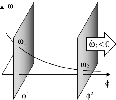
Figure 3: The figure shows the evolution of the second brane for the initial condition $\dot{\omega}_{2}<0$. The second brane is forced to evolve towards the fixed point $(\omega_{2},\dot{\omega}_{2})=0$ regardless of the evolution of the first brane.

Then, regardless the evolution of the first brane, the second brane will always continue moving to the right ($\dot{\omega}_{2}<0$ for all times). This can be seen most easily by rewriting Eq. (43) in the form

$$2H\dot{\omega}_{2} = -\ddot{\omega}_{2}-2\frac{\alpha_{2}^{2}}{\omega_{2}}(\dot{\omega}_{2})^{2}-\frac{1}{6}\omega_{2}a^{2}\tilde{R}$$ (46)

$$-\frac{\kappa_{5}^{2}}{24}\omega_{2}^{3}\sigma_{2}a^{2}(1-3s_{2})\rho_{2},$$

and proving that the right hand side remains always negative: Observe that for $\dot{\omega}_{2}$ to change signs it is necessary to have $\ddot{\omega}_{2}$ positive. Note also, from Eq. (45), that near $\dot{\omega}_{2}=0$ the Ricci scalar $\tilde{R}$ becomes positive. From these two observations we deduce that the right hand side of (46) is always negative (here we are making the additional assumption that $s_{2}\leqslant 1/3$, which includes matter, radiation, and cosmological constant dominated universes). The later is an important result for BPS braneworlds: in the low energy regime, the second brane is generally expected to evolve towards the fixed point $(\omega_{2},\dot{\omega}_{2})=0$.

III.5 Decoupled branes

Notice that if the second brane has effectively evolved to a configuration near the fixed point $(\omega_{2},\dot{\omega}_{2})=0$, then the first brane evolution becomes independent of the second brane $\Sigma_{2}$. As a matter of fact, the Friedmann’s Eq. (44) reduces to

$$\left(H+\frac{\dot{\omega}_{1}}{\omega_{1}}\right)^{2}-\frac{\sigma_{1}K^{2}H^{2}}{2k\omega_{1}^{2}}=a^{2}\omega_{1}^{2}\frac{\kappa_{5}^{2}}{12}\,\sigma_{1}\rho_{1}.$$ (47)

(In the next section we shall see that current observations can further constrain the form of this equation). More generally, the first brane dynamics is affected only by the moduli $\omega_{1}$, and the braneworld system becomes described by the following single scalar-tensor theory:

$$S = \frac{3}{4\pi G_{*}}\int d^{4}x\sqrt{-\tilde{g}}\bigg{[}\frac{W^{2}}{12}\tilde{R}+\frac{k}{\sigma_{1}}(\tilde{\partial}\omega_{1})^{2}\bigg{]}$$ (48)

$$+S_{1}[\Psi_{1},\omega^{2}_{1}\,\tilde{g}_{\mu\nu}],$$

where now the factor $W^{2}$ is given by:

$$W^{2}=4k\int_{0}^{\omega_{1}}\frac{\omega}{\sigma}\,\,d\omega.$$ (49)

Let us emphasize here that $\omega_{2}=0$ could be either a singularity (as discussed in Sec. II.2.3) or an asymptotic state of the system.

IV Observational constraints

General Relativity is characterized for having constant couplings $A_{1}$ and $A_{2}$ [see Eq. (21)]. The parameterized post-Newtonian formalism for bi-scalar-tensor theories consists of analyzing the effects of varying couplings $A_{1}$ and $A_{2}$ on the gravitational interaction between different bodies. This analysis is usually done by studying relativistic corrections in powers of $1/c^{2}$ to Newton’s gravitational potential.

In this article we consider the first post-Newtonian (1PN) level, where the analysis is considered up to $1/c^{2}$ order. Also, we shall be concerned with interacting bodies localized at the same brane (let us say the first brane $\Sigma_{1}$), thus we only consider the effects of the coupling $A_{1}$. Recall that in Sec. III we saw that the second brane $\Sigma_{2}$ is generally expected to evolve towards the fixed point ($\omega_{2},\dot{\omega}_{2})=0$. In particular, this is the case for branes dominated by matter and radiation, so we may safely assume that at late cosmological times both branes are far enough apart and do not interact through scalar interchange (this has been verified numerically for the particular case of dilatonic braneworlds num-dil ).

IV.1 Eddington parameters

Let us start our analysis with a brief outline on the definition of the Eddington parameters. Consider the interaction between bodies localized at the first brane (and therefore affected by the coupling $A_{1}$) and express $\omega_{1}$ and $\omega_{2}$ about their cosmological values $\omega^{0}_{1}$ and $\omega^{0}_{2}$ as

$$\omega_{1}=\omega^{0}_{1}+\varphi_{1},\qquad\mathrm{and}\qquad\omega_{2}=\omega^{0}_{2}+\varphi_{2}.$$ (50)

Then, $A_{1}$ can be expanded in the form

$$A_{1}=A_{1}^{0}\left[1+\eta^{a}_{0}\varphi_{a}+\frac{1}{2}(\eta^{a}_{0}\eta^{b}_{0}+\beta^{ab}_{0})\varphi_{a}\varphi_{b}+\ldots\right],$$ (51)

where $\eta^{a}_{0}$ and $\beta^{ab}_{0}$ are the background cosmological values of the following quantities:

$$\eta^{a}=\frac{1}{A_{1}}\frac{\partial A_{1}}{\partial\omega_{a}},\qquad\mathrm{and}\qquad\beta^{ab}=D^{a}\eta^{b},$$ (52)

where $D^{a}\eta^{b}=\partial^{a}\eta^{b}-\gamma^{ab}_{c}\eta^{c}$ is the sigma-model covariant derivative of $\eta^{a}$ with connections $\gamma^{ab}_{c}$ (see Appendix A). From here on we omit the “$0$” label denoting quantities evaluated at their cosmological background values. The effects of $A_{1}$ on the gravitational interaction can now be studied in terms of $\varphi$-scalars exchange between bodies. For instance, if we compute the Schwarzchild metric for a body of mass $m$ taking into account the perturbations $\varphi_{1}$ and $\varphi_{2}$, we find

$$-g_{00} = 1-2\frac{G_{N}m}{r}+2\beta\left(\frac{G_{N}m}{r}\right)^{2}+\mathcal{O}\left(1/c^{6}\right),\quad$$ (53)

$$g_{ij} = \delta_{ij}\left[1+2\gamma\frac{G_{N}m}{r}\right]+\mathcal{O}\left(1/c^{4}\right),$$ (54)

where $G_{N}=G_{*}A_{1}^{2}$ is the Newton’s constant as measured by Cavendish experiments in the brane. In the previous equations we have introduced the two Eddington parameters $\beta$ and $\gamma$ as PN1 :

$$\gamma-1 = -\frac{2\eta^{2}}{1+\eta^{2}},$$ (55)

$$\beta-1 = \frac{1}{2}\frac{\beta^{ab}\eta_{a}\eta_{b}}{(1+\eta^{2})^{2}},$$ (56)

where $\eta^{2}=\eta_{a}\eta^{a}$ (indexes are raised and lowered by the sigma model metrics $\gamma^{ab}$ and $\gamma_{ab}$). The basic role of these quantities is to parameterize deviations to Einstein gravity at the first post-Newtonian level (see Appendix B for the definition of the second post-Newtonian level parameters).

IV.2 Braneworld’s Eddington parameters

In the specific case of our model, we can compute $\eta^{2}$ and $\beta^{ab}\eta_{a}\eta_{b}$ in terms of $\sigma$ and other quantities

$$\eta^{2} = \frac{1}{3}\left[1-\frac{\sigma_{1}}{2kA_{1}^{2}}\right],$$ (57)

$$\beta^{ab}\eta_{a}\eta_{b} = \frac{1}{9}\left(1-3\eta^{2}\right)\left[3\eta^{2}-2\alpha_{1}^{2}\left(1-3\eta^{2}\right)\right].$$ (58)

Before continuing the discussion, it will be useful to introduce a new parameter encoding information from the bulk geometry. Recalling the definitions of $W^{2}$ and $K^{2}$ in Eqs. (20) and (29) respectively, we define

$$\langle\alpha^{2}\rangle=\frac{1}{2}\frac{K^{2}}{W^{2}}.$$ (59)

Here $\langle\alpha^{2}\rangle$ can be interpreted as the average value of $\alpha^{2}$ over the bulk taking into account the background geometry; for instance, if the background’s geometry is strongly warped near $\Sigma_{1}$, we should expect $\langle\alpha^{2}\rangle$ to be small and close to the boundary value $\alpha_{1}^{2}$. In particular, if $\alpha$ is constant, then $\langle\alpha^{2}\rangle=\alpha_{1}^{2}=\alpha^{2}$, which corresponds to dilatonic braneworlds. We shall come back to the geometrical meaning of $\langle\alpha^{2}\rangle$ in Sec. IV.5.

To further simplify our analysis, observe from Eq. (55) that if $\gamma\simeq 1$ then $\eta^{2}\simeq 0$. Thus, neglecting second order terms in $\eta^{2}$ on Eqs. (55) and (56), we can reexpress the post-Newtonian parameters simply as

$$1-\gamma = \frac{4}{3}\langle\alpha^{2}\rangle+\frac{2}{3}\frac{\omega^{2}_{2}\sigma_{1}}{\omega^{2}_{1}\sigma_{2}},$$ (60)

$$1-\beta = \frac{1}{9}\left(\alpha_{1}^{2}-\langle\alpha^{2}\rangle\right)-\frac{1}{18}\frac{\omega^{2}_{2}\sigma_{1}}{\omega^{2}_{1}\sigma_{2}}.$$ (61)

Notice that $\gamma$ is related to the global configuration of the system, while $\beta$ encodes departures of the brane parameter $\alpha_{1}^{2}$ from $\langle\alpha^{2}\rangle$. In particular, if the branes are far apart, we find:

$$1-\gamma = \frac{4}{3}\langle\alpha^{2}\rangle,$$ (62)

$$1-\beta = \frac{1}{9}\left(\alpha_{1}^{2}-\langle\alpha^{2}\rangle\right).$$ (63)

In what follows, we study the current observational constraints on these parameters.

IV.3 Solar-system tests

Current solar-system tests place tight constraints on the 1PN level parameters. A few of the most relevant tests constraining these parameters are: The observations on the perihelion shift of Mercury, which implies Mercury

$$|2\gamma-\beta-1|<3\times 10^{-3},$$ (64)

the lunar laser ranging experiment, which provides the value Lunar

$$4\beta-\gamma-3=(-0.7\pm 1)\times 10^{-3},$$ (65)

the light deflection measured by the very long baseline interferometry experiment VLB

$$|\gamma-1|<4\times 10^{-4},$$ (66)

and the measurement of the time delay variation to the Cassini spacecraft near the solar conjunction, which gives the impressive result Cassini

$$\gamma-1=(2.1\pm 2.3)\times 10^{-5}.$$ (67)

In the present analysis it will be enough to consider only the constraint shown in Eq. (67). Furthermore, since in our theory $1-\gamma$ is always positive, we can reinterpret this bound as $1-\gamma<2\times 10^{-6}$. This imposes the following two inequalities

$$\frac{\omega^{2}_{2}\sigma_{1}}{\omega^{2}_{1}\sigma_{2}} < 3\times 10^{-6},$$ (68)

$$\langle\alpha^{2}\rangle < 1.5\times 10^{-6}.$$ (69)

Bound (68) gives us information regarding the relative positions of both branes on the background, however it does not constrain the geometry of the system. For example, if $\sigma(\phi)$ is a slowly varying function of $\phi$ in the bulk (between both branes), then the warp factor $\omega(z)$ must vary quickly from one brane to the other (a strongly warped geometry). Nevertheless, it may be possible to have configurations where the warp factor does not necessarily vary much from one brane to the other, but $\sigma(\phi)$ does. In any case, it is important to note that Eq. (68) is in good agreement with our analysis made on the cosmological evolution of the branes, where we found that the second brane has an attractor behavior to the state $(\omega_{2},\dot{\omega}_{2})=0$. In what follows we assume that the terms involving $\omega_{2}$ in Eqs. (60) and (61) can be safely neglected, and continue using Eqs. (62) and (63) instead.

Let us now move to inequality (69). This bound constrains the average value of $\alpha^{2}$ in the bulk, and can be used to discard many possible shapes for the brane-potential $\sigma(\phi)$. Furthermore, observe that the Friedmann’s Eq. (47) can be rewritten in the form

$$\left(H+\frac{\dot{\omega}_{1}}{\omega_{1}}\right)^{2}=2\,\langle\alpha^{2}\rangle H^{2}+a^{2}\omega_{1}^{2}\frac{\kappa_{5}^{2}}{12}\,\sigma_{1}\rho_{1}.$$ (70)

Neglecting the term proportional to $\langle\alpha^{2}\rangle$ and defining the proper Hubble parameter $\mathcal{H}\equiv(H+\dot{\omega}_{1}/\omega_{1})/a^{2}\omega_{1}^{2}$ (as it would be measured by an observer at the $\Sigma_{1}$ brane frame), we arrive at the simple expression

$$\mathcal{H}^{2}=\frac{\kappa_{5}^{2}}{12}\,\sigma_{1}\rho_{1}=\frac{8\pi}{3}G_{N}\rho_{1},$$ (71)

where we have used $\sigma_{1}\simeq 2kA_{1}^{2}$. This corresponds to the Friedmann’s equation with a varying Newton’s constant $G_{N}\propto\sigma(\phi^{1})$. In other words, during late cosmological times, solar system tests imply that our universe’s evolution must be described by the conventional Friedmann’s equation.

IV.4 Binary-pulsar tests

Solar-system tests impose mild constraints on the $\beta$ parameter and, consequently, on $\alpha^{2}_{1}$. For instance, bound (65) gives $\alpha_{1}^{2}<3.9\times 10^{-3}$, which is 3 orders of magnitude weaker than (69). It is possible, however, to improve the bounds on $\alpha^{2}_{1}$ by considering binary-pulsar tests; general relativity has shown to be very successful in describing the physics of binary-pulsars. For example, in the case of the Hulse-Taylor binary-pulsar PSR B1913+16, three relativistic parameters have been determined with great accuracy pulsar-exp : the Einstein time delay parameter $\gamma_{T}$, the periastron advance $\dot{\omega}$, and the rate of change of the orbital period $\dot{P}$. It is well known that the strong field conditions offered by binary-pulsars make the moduli to behave nonperturbatively around them Pulsar1 ; Pulsar2 , modifying the predictions on $\gamma_{T}$, $\dot{\omega}$, and $\dot{P}$ made by GR. This offers strong constraints on $\beta$ and $\gamma$; in particular, in the region $\beta<0$ the following result holds strong-field

$$\frac{\beta-1}{\gamma-1}<1.1.$$ (72)

Then, using Eqs. (62) and (63), we obtain

$$\alpha_{1}^{2}<13.2\,\langle\alpha^{2}\rangle,$$ (73)

which is a much stronger bound on the brane parameter $\alpha_{1}^{2}$. Putting together bounds (73) and (69) we can restrict the parameter space for braneworld models considerably. Fig. 4 summarizes the discussed bounds on the parameters of the theory.

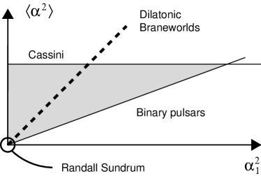
Figure 4: The figure sketches the constrained parameter space spanned by $\alpha_{1}^{2}$ and $\langle\alpha^{2}\rangle$. The Randall-Sundrum model corresponds to the point $(\alpha_{1}^{2},\langle\alpha^{2}\rangle)=0$, while dilatonic braneworlds are represented by the curve $\langle\alpha^{2}\rangle=\alpha_{1}^{2}$.

IV.5 Geometrical interpretation of the constraints

We now would like to extract some meaningful information out of the constrained parameters $\alpha_{1}^{2}$ and $\langle\alpha^{2}\rangle$. Let us start by observing that $\langle\alpha^{2}\rangle$ measures the way in which $\sigma$ varies as a function of the warp factor $\omega$. If the $\Sigma_{1}$ brane is located in a strongly warped region, where $\omega$ varies quickly in terms of $z$ while $\sigma$ does it slowly (as in the Randall-Sundrum model), then we should generally expect $\langle\alpha^{2}\rangle$ to be a small parameter. In contrast, if $\Sigma_{1}$ is in a region where $\sigma$ varies importantly in terms of $z$ but $\omega$ does not, then, in general, $\langle\alpha^{2}\rangle$ can be expected to acquire arbitrary large values. To be more precise, let us parameterize $\sigma$ as a function of $\omega$ (which has to be a monotonically decreasing function of $\omega$), and consider the profile shown in Fig. 5:

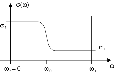
Figure 5: The figure shows a generic potential $\sigma$ as a function of $\omega$. The parameter $\omega_{0}$ can be adjusted to analyze different cases near the first brane (where $\omega=\omega_{1}$).

The function $\sigma$ varies slowly in the region $\omega_{2}<\omega<\omega_{0}$, with a value $\sigma\sim\sigma_{2}$. Then, it has a steep variation around the value $\omega=\omega_{0}$. And finally, it returns to a slowly varying function in the region $\omega_{0}<\omega<\omega_{1}$, with $\sigma\sim\sigma_{1}$. Additionally, assume that $\sigma_{2}\gg\sigma_{1}$ which is generally the case if $\omega_{2}=0$. Then $K^{2}$ and $W^{2}$ can be approximated to the following expressions:

$$K^{2} \simeq 2\frac{\omega_{0}^{2}}{\sigma_{1}},$$ (74)

$$W^{2} \simeq 2\frac{\omega_{1}^{2}-\omega_{0}^{2}}{\sigma_{1}}+2\frac{\omega_{0}^{2}}{\sigma_{2}}.$$ (75)

Thus if $\omega_{1}\gg\omega_{0}$, that is, if the geometry around the brane is strongly warped, then we find

$$\langle\alpha^{2}\rangle\sim\frac{1}{2}\frac{\omega_{0}^{2}}{\omega_{1}^{2}}\ll 1,$$ (76)

otherwise if $\omega_{1}\sim\omega_{0}$, then we find

$$\langle\alpha^{2}\rangle\sim\frac{1}{2}\frac{\sigma_{2}}{\sigma_{1}}\gg 1.$$ (77)

This example shows two extreme cases concerning the geometry around the first brane $\Sigma_{1}$. The constraint (69) thus allows us to infer that the geometry around the braneworld $\Sigma_{1}$ is highly warped to agree with observations.

We can also ask about the behavior of $\sigma$ around the brane. In this case, the comparison between $\alpha_{1}^{2}$ and $\langle\alpha^{2}\rangle$ tells us the growth of $\sigma$ around the brane. For example, if $\alpha_{1}^{2}=\langle\alpha^{2}\rangle$, the potential corresponds to the dilatonic case $\sigma\propto\exp[\alpha\phi]$ (with $\alpha$ a constant), whereas if $\alpha_{1}^{2}<\langle\alpha^{2}\rangle$, the tendency of $\sigma$ is to grow faster than the dilatonic case, and if $\alpha_{1}^{2}>\langle\alpha^{2}\rangle$, then the tendency is to grow slower. Fig. 6 shows the different cases.

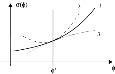
Figure 6: The figure shows different behaviors for $\sigma(\phi)$ about the first brane position $\phi^{1}$. The curves are: Curve 1, $\alpha_{1}^{2}=\langle\alpha^{2}\rangle$ (dilatonic braneworlds); Curve 2, $\alpha_{1}^{2}<\langle\alpha^{2}\rangle$; Curve 3, $\alpha_{1}^{2}>\langle\alpha^{2}\rangle$.

At present, bound (73) is unable to provide evidence in favor on any of these cases.

IV.6 Can we live in the second brane?

Up to now we have considered the case of tests being performed at the first brane. We can repeat our analysis and compute the Eddington’s parameters for the second brane $\Sigma_{2}$. In this case it is found:

$$\eta^{2}=\frac{1}{3}\left[1+\frac{\sigma_{2}}{2kA_{2}^{2}}\right],$$ (78)

which, after considering the cosmological evolution of the branes provides the result: $\gamma-1\simeq-2$. We therefore conclude that our universe cannot be localized to the second brane.

V Conclusions

In this paper we have considered the low energy regime of 5D braneworld models with a bulk scalar field. The present setup (BPS braneworlds) included the Randall-Sundrum model and dilatonic braneworlds as particular cases [different models are distinguished by the brane potential $\sigma(\phi)$]. We discussed the way in which solar system and binary pulsar tests can be used to constrain the bulk geometry and the configuration of the branes. For this, it was first necessary to understand the cosmological behavior of the branes; we found that the negative tension brane is generally expected to evolve towards a null warp-factor state, meaning that at late cosmological times both branes end up interacting weakly.

At late cosmological times the positive tension brane is well described by a single scalar-tensor theory of gravity [see Eq. (48)]. Then, having defined the parameter $\alpha=\sigma^{-1}\partial_{\phi}\sigma$, it was found that the post-Newtonian Eddington parameters $\beta$ and $\gamma$ can be expressed in terms of two brane parameters, $\alpha_{1}=\alpha(\phi^{1})$ and $\langle\alpha^{2}\rangle$, containing information of the bulk geometry near the first brane. In terms of these parameters, dilatonic braneworlds corresponds to the case: $\langle\alpha^{2}\rangle=\alpha_{1}^{2}=\,$const.; whereas the Randall-Sundrum model corresponds to: $\langle\alpha^{2}\rangle=\alpha_{1}^{2}=0$. We found two constraints: $\langle\alpha^{2}\rangle<1.5\times 10^{-6}$ and $\alpha_{1}^{2}<13.2\,\langle\alpha^{2}\rangle$, which allowed us to infer that the geometry around the braneworld is strongly warped [see Eq. (76)].

The analysis made in this paper should allow a better understanding of generic 5D braneworld models and their low energy phenomenology. The present results can be used together with other tests to further constrain the role of $\phi$ (the bulk scalar field), as well as other moduli, in the 4D standard model of physics. Examples of this are the possibility of $\phi$ being a source for inflation infl , the variation of constants variconst , a chameleon field chameleon , or dark energy. In the later case, it would be interesting to explore the reconstruction of the shape of $\sigma(\phi)$ as a function of $\phi$ out of measurements on the dark energy evolution reconst1 ; reconst2 .

Appendix A Einstein’s frame sigma model

Here we provide the Einstein’s frame sigma-model connections $\gamma_{c}^{ab}$. They are given by the expression

$$\gamma_{c}^{ab}=\frac{1}{2}\gamma_{cd}\left[\partial^{a}\gamma^{db}+\partial^{b}\gamma^{ad}-\partial^{d}\gamma^{ab}\right],$$ (79)

where derivatives $\partial^{a}$ are made with respect to $\omega_{a}$. The nonzero connections are

$$\gamma^{11}_{1} = \frac{2}{\omega_{1}}\left[\alpha_{1}^{2}-\frac{2kA_{1}^{2}}{\sigma_{1}}+\frac{2kA_{1}^{2}\alpha_{1}^{2}W^{2}}{\sigma_{1}K^{2}}\right],$$

$$\gamma^{22}_{2} = \frac{2}{\omega_{2}}\left[\alpha_{2}^{2}+\frac{2kA_{2}^{2}}{\sigma_{2}}-\frac{2kA_{2}^{2}\alpha_{1}^{2}W^{2}}{\sigma_{2}K^{2}}\right],$$

$$\gamma^{11}_{2} = \frac{4k\alpha_{1}^{2}\omega_{2}}{\sigma_{1}K^{2}},\qquad\gamma^{22}_{1}=-\frac{4k\alpha_{2}^{2}\omega_{1}}{\sigma_{2}K^{2}},$$

$$\gamma^{12}_{1} = \frac{2k\omega_{2}}{\sigma_{2}W^{2}},\qquad\gamma^{12}_{2}=-\frac{2k\omega_{1}}{\sigma_{1}W^{2}}.$$ (80)

Appendix B 2PN level parameters

At the second post-Newtonian (2PN) level (order $1/c^{4}$) it is possible to introduce two new parameters $\epsilon$ and $\zeta$, which play a similar role to $\beta$ and $\gamma$ 2PN . Here we consider their definition for completeness. These parameters are

$$\epsilon = \frac{\beta^{abc}\eta_{a}\eta_{b}\eta_{c}}{(1+\eta^{2})^{3}},$$ (81)

$$\zeta = \frac{\beta^{ac}\beta_{c}^{b}\eta_{a}\eta_{b}}{(1+\eta^{2})^{3}},$$ (82)

where $\beta^{abc}=D^{a}D^{b}\eta^{c}$. A straightforward but tedious calculation shows that

$$\beta^{abc}\eta_{a}\eta_{b}\eta_{c} = -\frac{6}{1-3\eta^{2}}\left(\beta^{ab}\eta_{a}\eta_{b}\right)^{2}$$ (83)

$$-\frac{8}{9}\alpha_{1}^{2}\left(1-3\eta^{2}\right)^{2}\left[1-2\alpha_{1}^{2}\frac{W^{2}}{K^{2}}\right]$$

$$-\frac{16}{27}\alpha_{1}^{2}\left(1-3\eta^{2}\right)^{3}\frac{\partial\alpha_{1}}{\partial\phi^{1}},$$

$$\beta^{ac}\beta_{c}^{b}\eta_{a}\eta_{b} = -\frac{1}{3}\left(1-3\eta^{2}\right)\beta^{ab}\eta_{a}\eta_{b}$$ (84)

$$-\frac{2}{9}\alpha_{1}^{2}\left(1-3\eta^{2}\right)^{3}\left[1-2\alpha_{1}^{2}\frac{W^{2}}{K^{2}}\right]$$

$$+\frac{4}{27}\alpha_{1}^{4}\left(1-3\eta^{2}\right)^{2}\frac{\omega^{2}_{2}\sigma_{1}}{\omega^{2}_{1}\sigma_{2}}.$$

Using Eqs. (60) and (61), and the fact that $\eta^{2}\simeq 0$, we find

$$\epsilon = \frac{2}{3}(1-\beta)+\frac{4}{27}\alpha_{1}^{2}\frac{\omega^{2}_{2}\sigma_{1}}{\omega^{2}_{1}\sigma_{2}}$$ (85)

$$+\frac{2}{9}\frac{\alpha_{1}^{2}}{\langle\alpha^{2}\rangle}\left(\alpha_{1}^{2}-\langle\alpha^{2}\rangle\right),$$

$$\zeta = -24(1-\beta)^{2}-\frac{16}{27}\alpha_{1}^{2}\frac{\partial\alpha_{1}}{\partial\phi}$$ (86)

$$+\frac{8}{9}\frac{\alpha_{1}^{2}}{\langle\alpha^{2}\rangle}\left(\alpha_{1}^{2}-\langle\alpha^{2}\rangle\right).$$

In principle, these parameters can be used to further constrain 5D braneworld models.

References

- (1) D. Langlois, Prog. Theor. Phys. Suppl. 148, 181 (2003).
- (2) R. Maartens, Living Rev. Relativity 7, 7 (2004).
- (3) Ph. Brax, C. van de Bruck, and A.C. Davis, Rep. Prog. Phys. 67, 2183 (2004).
- (4) J. Garriga and T. Tanaka, Phys. Rev. Lett. 84, 2778 (2000).
- (5) T. Chiba, Phys. Rev. D 62, 021502 (2000).
- (6) T. Tanaka and X. Montes, Nucl. Phys. B 582, 259 (2000).
- (7) P. Binetruy, C. Deffayet, and D. Langlois, Nucl. Phys. B 615, 219 (2001).
- (8) Ph. Brax, C. van de Bruck, A.C. Davis, and C.S. Rhodes, Phys. Lett. B 531, 135 (2002).
- (9) P. Kanti, K.A. Olive, and M. Pospelov, Phys. Lett. B 538, 146 (2002).
- (10) P. Kanti, S.C. Lee, and K.A. Olive, Phys. Rev. D 67, 024037 (2003).
- (11) Gonzalo A. Palma and Anne-Christine Davis, Phys. Rev. D 70, 064021 (2004).
- (12) Gonzalo A. Palma and Anne-Christine Davis, Phys. Rev. D 70, 106003 (2004).
- (13) C. Will, Living Rev. Relativity 4, 4 (2001).
- (14) A.S. Eddington, The Mathematical Theory of Relativity (Cambridge University Press, Cambridge, England, 1993).
- (15) B. Bertotti, L. Iess and P. Tortora, Nature (London) 425, 374 (2003).
- (16) J.G. Williams, X.X. Newhall, and J.O. Dickey, Phys. Rev. D 53, 6730 (1996).
- (17) Thibault Damour and Gilles Esposito-Farese, Phys. Rev. D 54, 1474 (1996).
- (18) Thibault Damour and Gilles Esposito-Farese, Phys. Rev. D 58, 042001 (1998).
- (19) L. Randall and R. Sundrum, Phys. Rev. Lett. 83 3370 (1999).
- (20) L. Randall and R. Sundrum, Phys. Rev. Lett. 83 4690 (1999).
- (21) A. Lukas, B.A. Ovrut, K. Stelle and D. Waldram, Phys. Rev. D 59, 086001 (1999).
- (22) E.E. Flanagan, S.H.H. Tye and I. Wasserman, Phys. Lett. B 522, 155 (2001).
- (23) O. DeWolfe, D.Z. Freedman, S.S. Gubser, and A. Karch, Phys. Rev. D 62, 046008 (2000).
- (24) E. Bergshoeff, R. Kallosh and A.V. Proeyen, J. High Energy Phys. 10 (2000) 033.
- (25) P. Binetruy, J.M. Cline, and C. Grojean, Phys. Lett. B 489, 403 (2000).
- (26) Ph. Brax and A.C. Davis, Phys. Lett. B 497, 289 (2001); J. High Energy Phys. 05 (2001) 007.
- (27) C. Csaki, J. Erlich, C. Grojean, and T.J. Hollowood, Nucl. Phys. B 584, 359 (2000).
- (28) D. Youm, Nucl. Phys. B 596, 289 (2001).
- (29) Ph. Brax, C. van de Bruck, A.C. Davis, and C.S. Rhodes, Phys. Rev. D 67, 023512 (2003).
- (30) T. Damour and G. Esposito-Farese, Classical Quantum Gravity 9, 2093 (1992).
- (31) I.I. Shapiro, in General Relativity and Gravitation Vol. 12, edited by N. Ashby, D.F. Bartlett, and W. Wyss (Cambridge University Press, Cambridge, England, 1990), p. 313.
- (32) T.M. Eubanks et al., Am. Phys. Soc., Abstract K 11, 05 (1997).
- (33) J.M. Weisberg and J.H. Taylor, ASP Conf. Proc. 302, 93 (2003). astro-ph/0211217.
- (34) Gilles Esposito-Farese, AIP Conf. Proc. 736, 35 (2004). gr-qc/0409081.
- (35) C. Ringeval, Ph. Brax, C. van de Bruck and A.C. Davis, astro-ph/0509727.
- (36) G.A. Palma, Ph. Brax, A.C. Davis and C. van de Bruck, Phys. Rev. D 68, 123519 (2003).
- (37) Ph. Brax, C. van de Bruck and A.C. Davis, J. Cosmol. Astropart. Phys. 11 (2004) 004.
- (38) B. Boisseau, G. Esposito-Farese, D. Polarski, A.A. Starobinsky, Phys. Rev. Lett. 85, 2236 (2000).
- (39) G. Esposito-Farese and D. Polarski, Phys. Rev. D 63, 063504 (2001).
- (40) T. Damour and G. Esposito-Farese, Phys. Rev. D 53, 5541 (1996).