DFTT 29/05

SISSA 87/2005/FM

PTA/05-72

MIT-CPT-3705

gef-th-9/05

Potts correlators and the static three-quark potential

M. Caselle^a, G. Delfino^b, P. Grinza^c, O. Jahn^d and N. Magnoli^e

^a Dipartimento di Fisica Teorica dell’Università di Torino and I.N.F.N.,

via P.Giuria 1, I-10125 Torino, Italy

e–mail:          caselle@to.infn.it

^b International School for Advanced Studies (SISSA)

via Beirut 2-4, 34014 Trieste, Italy

INFN sezione di Trieste

e–mail:          delfino@sissa.it

^c Laboratoire de Physique Théorique et Astroparticules, Université Montpellier II,

Place Eugène Bataillon, 34095 Montpellier Cedex 05, France

e–mail:          grinza@lpta.univ-montp2.fr

^dCenter for Theoretical Physics, MIT, Cambridge, MA 02139, USA

e–mail:          jahn@mit.edu

^e Dipartimento di Fisica, Università di Genova and I.N.F.N.,

via Dodecaneso 33, I-16146 Genova, Italy

e–mail:          magnoli@ge.infn.it

We discuss the two- and three-point correlators in the two-dimensional three-state Potts model in the high-temperature phase of the model. By using the form factor approach and perturbed conformal field theory methods we are able to describe both the large distance and the short distance behaviours of the correlators. We compare our predictions with a set of high precision Monte-Carlo simulations (performed on the triangular lattice realization of the model) finding a complete agreement in both regimes. In particular we use the two-point correlators to fix the various non-universal constants involved in the comparison (whose determination is one of the results of our analysis) and then use these constants to compare numerical results and theoretical predictions for the three-point correlator with no free parameter. Our results can be used to shed some light on the behaviour of the three-quark correlator in the confining phase of the (2+1)-dimensional SU(3) lattice gauge theory which is related by dimensional reduction to the three-spin correlator in the high-temperature phase of the three-state Potts model. The picture which emerges is that of a smooth crossover between a $\Delta$ type law at short distances and a Y type law at large distances.

1 Introduction

The aim of this paper is to study the three-point correlator in the ${\mathbb{Z}}_{3}$ Potts model outside the critical point. In particular we shall study the thermal perturbation of the model, in the high-temperature phase (i.e. the phase in which the symmetry is unbroken and the magnetization is zero). We shall first discuss the two-point function and compare it with high precision numerical simulations in order to fix all the normalizations and the non-universal quantities which appear in the three-point function. Then we shall address the three-point function and compare it again with numerical simulations. Thanks to the preliminary analysis of the two-point function this comparison will not require any fitting procedure but will be a direct and absolute comparison between theoretical predictions and numerical results.

On the theoretical side we shall study both the two- and the three-point correlators with two different tools.

• The form factor approach which is essentially a large distance expansion. This approach requires exact integrability, a condition which is indeed fulfilled by the scaling ${\mathbb{Z}}_{3}$ Potts model.

• The perturbative expansion around the conformal fixed point which is essentially a short distance expansion and is completely general, meaning that no specific integrability property of the perturbation under study is needed.

From a theoretical point of view this is a rather interesting challenge:

• In the large distance regime (where the form factor approach is expected to hold) the strong coupling expansion suggests the existence of an additional midpoint, inside the triangle spanned by the three spins of the correlators, where the strong coupling paths emerging from the three spins converge and join. The appearence of this new point is a novelty with respect to the well known form factor calculation for the two point functions. The way in which it is obtained is non-trivial and is one of the interesting features of our analysis.

• Similarly it is the first time that the approach of the perturbative, infrared safe, expansion around the conformal solution is used for a three point function. This required some non-trivial extension of the techniques used in previous works on the two-point functions.

From a physical point of view the scenario which emerges (which strongly resembles what one finds when looking at the three-quark potential in lattice gauge theories (LGT), a correspondence which we shall discuss in detail below) is a smooth crossover, as the distance among the three points increases, from a short distance behaviour in which the three point function is dominated by the three spin-spin interactions along the edges of the triangle to a large distance behaviour in which the strong coupling expectation (the three spins joined by a path of minimal length) is fully realized.

This scenario is confirmed by the numerical simulations which turn out to be in remarkable agreement with our theoretical results. Indeed the important consequence of having exact analytic results for the two expansions is that we are able to compare our predictions with triangles of any size, both smaller and larger than the correlation length. Moreover, even if in the following we shall mainly perform our comparisons in the equilateral case, we can obtain analytic predictions for triangles of any shape, thus allowing a very selective test of our results.

Besides a better understanding of the three-state Potts model a second important motivation which we had in mind addressing the present problem is to use our results to shed some light on the behaviour of the three-quark potential in SU(3) LGT’s. Indeed by dimensional reduction the (2+1)-dimensional SU(3) LGT can be mapped into the two-dimensional three-state Potts model and in particular the three-quark free energy is mapped into the three-point function of the Potts model (we shall discuss in detail this correspondence in sect.7 below). An important open problem in the study of the three-quark potential is to understand if the three-quark correlator follows the so called “Y” or “$\Delta$” law (for a discussion of these laws see again sect.7 below). Our results on the three-state Potts model suggest that the right picture is a smooth crossover between the two laws. At short distance, i.e. for interquark distances smaller than the correlation length, the three-quark potential is well described by the $\Delta$ law, which is indeed exact at the critical point (i.e. when the correlation length goes to infinity), while at large distances the correct description is the Y law, which becomes exact in the strong coupling limit, i.e. for interquark distances much larger than the correlation length. This mixed behaviour agrees with the results of some recent simulations performed directly in the gauge model [42].

This paper is organized as follows. Sect.2 contains a general discussion of the three-state Potts model both on the lattice and in the continuum and its CFT description at the critical point. In sect.3 we discuss the form factor analysis of the large distance expansion both for the two- and the three-point functions. Then in sect.4 we shall compare these predictions with a set of high precision Monte-Carlo simulations performed on a triangular lattice. Sect.5 is then devoted to the study of the short distance perturbative expansion which is then compared with the Monte-Carlo data in sect.6. In sect.7 we shall then briefly comment on the implications of our results for the study of barionic states in LGT. Two appendices conclude the paper. The first contains some technical steps we omit in the main text, while the second is devoted to universal amplitude ratios.

2 The three-state Potts model

The two-dimensional, isotropic, nearest-neighbor, three-state Potts model at temperature $T$ on a lattice $\Lambda$ is defined by the partition function

$$Z=\sum_{\{s_{n}\}}e^{-\beta{\cal H}}$$ (1)

with the Hamiltonian

$${\cal H}=J\sum_{\langle nn^{\prime}\rangle}(1-\delta_{s_{n}s_{n^{\prime}}})$$ (2)

where $s_{n}=0,1,2$ are ${\mathbb{Z}}_{3}$-valued variables on each site, $n\in\Lambda$, $\beta=(k_{B}T)^{-1}$, and $\langle nn^{\prime}\rangle$ denotes pairs of nearest-neighbor sites [1]. The symmetry group of the Potts Hamiltonian is $S_{3}$, the permutation group of $3$ objects. In the following we shall study in particular the case in which $\Lambda$ is a regular triangular lattice with honeycomb boundary conditions.

This choice is motivated by the fact that in the following we shall mainly be interested in the three-point function of the model, for which a more symmetric choice of arguments is possible on a triangular lattice. Notice however that most of our theoretical results are obtained in the continuum limit theory and hence, once the non-universal, lattice dependent, normalizations are fixed, hold for any lattice $\Lambda$. A general introduction to the Potts model can be found in the review by Wu [2]. Recently a set of interesting results (series expansions and exact free energy calculation on strips) for the triangular lattice realization of the model in which we are interested appeared in a series of papers (see in particular [3],[4] and references therein) to which we refer the interested reader.

The model is known to have a second order phase transition for a critical value $T_{c}$ of the temperature which separates the high-temperature, symmetric phase from the low-temperature one in which the symmetry is broken and a spontaneous magnetization appears. In the following we shall be interested in the symmetric high-temperature phase. This is due to the fact that (as we shall discuss in the last section) we plan to use our results to better understand the behaviour of the baryonic states in LGT, and the confining phase of the SU(3) LGT is mapped by dimensional reduction to the high-temperature phase of the $3$-state Potts model.

Assuming that a single phase transition point exists in the model, the critical temperature can be obtained exactly even for the triangular lattice by using duality and the star triangle relation which, combined together, lead to an algebraic equation for $T_{c}$ [5]. Defining $a=e^{\beta}$ we have

$$a^{3}-3a-1=0$$ (3)

whose unique positive solution is

$$a=\cos(2\pi/9)+\sqrt{3}\sin(2\pi/9)=1.879385...$$ (4)

to which the critical value $\beta_{c}=0.6309447...$ corresponds.

At the critical point the model is described by a minimal (non-diagonal) CFT with central charge $c=4/5$. It may be useful to briefly describe this model. It is indeed the simplest example of a non-diagonal minimal model of the Virasoro series [6]. However it can be also realized as the simplest diagonal minimal model of the so called $W_{3}$ algebra [7].

Its operator content is composed by six primary fields, which however, due to the non-diagonal nature of the model, lead to a larger number of operators when the analytic and antianalytic sector are combined. Using the standard CFT notation $(r,s;r^{\prime},s^{\prime})$ which corresponds to the conformal dimensions $(h_{r,s},h_{r^{\prime},s^{\prime}})$ for the field, with $h_{r,s}$ given by

$$h_{r,s}=\frac{(6r-5s)^{2}-1}{120}$$ (5)

the most relevant operator in the energy sector is $\epsilon=(2,1;2,1)$ with scaling dimension $X_{\epsilon}=2h_{2,1}=4/5$, while the most relevant operators in the magnetic sector are the doublet $\sigma$ and $\bar{\sigma}$, of type $(3,3;3,3)$, with scaling dimension $X_{\sigma}=X_{\bar{\sigma}}=2h_{3,3}=2/15$.

The nice feature of the $W_{3}$ description is that the operator content is composed by four fields only (besides the identity) and all the higher fields appear as secondary fields in the $W_{3}$ conformal families.

3 Large distance expansion

In this section we shall obtain the large distance behaviour of the two- and three-point functions of the model. As a preliminary step in this direction we shall first obtain an explicit expression for the two-particle form factors.

3.1 Form factors of order/disorder operators in three-state Potts model

The continuum limit description of the model in which we are interested is given by the thermal perturbation of the above discussed CFT, i.e.

$$S=S_{\textrm{\tiny CFT}}+\tau\int\textrm{d}^{2}x\;\epsilon(x)$$ (6)

and belongs to the class of integrable QFTs [8].

In the computation of form factors it is fundamental to establish which is the nature of the basis of asymptotic states of the theory, i.e. which are the particle excitations which come into play. This is the main difference between the high-temperature and low-temperature phase of the model.

At $\tau<0$ there are three degenerate vacua and the excitations are the kinks $K_{j,j\pm 1}$, with $j=1,2,3$, which interpolate between the ground state $j$ and the ground state $j+1(\textrm{mod}3)$. Form factors in this regime can be found in [9].

At $\tau>0$ the ground state is unique, the ${\mathbb{S}}_{3}\simeq{\mathbb{Z}}_{2}\times{\mathbb{Z}}_{3}$ symmetry is unbroken and its simplest realization is in terms of a doublet of particles $A$ and $\bar{A}$ transforming as

$$\Omega A=\omega A,\ \ \ \ \Omega\bar{A}=\omega^{-1}\bar{A};\ \ \ \ \ \ \ \ \mathcal{C}A=\bar{A}$$ (7)

where $\Omega$ is the ${\mathbb{Z}}_{3}$ generator, $\mathcal{C}$ the charge conjugation operator and $\omega=e^{2\pi i/3}$. The ${\mathbb{Z}}_{3}$ symmetry allows the existence of the fusion process

$$AA\to\bar{A}.$$ (8)

The two particle $S$-matrix for this integrable model turns out to be [10, 11]

$$|A(\theta_{1})A(\theta_{2})\rangle = u(\theta)|A(\theta_{2})A(\theta_{1})\rangle$$

$$|A(\theta_{1})\bar{A}(\theta_{2})\rangle = t(\theta)|A(\theta_{2})\bar{A}(\theta_{1})\rangle$$ (9)

where $\theta=\theta_{1}-\theta_{2}$ and

$$u(\theta)=t(i\pi-\theta)=\frac{\sinh\frac{1}{2}(\theta+\frac{2\pi i}{3})}{\sinh\frac{1}{2}(\theta-\frac{2\pi i}{3})}.$$ (10)

The pole present in the amplitude $u(\theta)$ located at $\theta=\frac{2\pi i}{3}$ corresponds to the bound state (8).

For the reasons discussed above, in the following we shall concentrate on the $\tau>0$ case. The symmetry of the model implies the presence of a doublet of spin operators $\sigma$ and $\bar{\sigma}$ which form a two-dimensional representation of ${\mathbb{S}}_{3}$ and transform as $A$ and $\bar{A}$ in (7). Duality also requires the existence of a doublet of disorder operators $\mu$, $\bar{\mu}$.

The $n$-particle form factors of a given operator $\Phi$ are defined as

$$F_{a_{1},\dots,a_{n}}^{\Phi}(\theta_{1},\dots,\theta_{n})=\langle 0|\Phi(0)|A_{a_{1}}(\theta_{1})\dots A_{a_{n}}(\theta_{n})\rangle$$ (11)

with the indices $a_{i}$ referring to particle species. They satisfy a set of axioms which can be used to compute them explicitly [12, 13, 14].

In the following we shall be interested in the two-particle form factors for the $\sigma$ ($\bar{\sigma}$) and $\mu$ ($\bar{\mu}$) operators [15, 9, 16]. The spin operator satisfy (we recall that $\sigma$ and $\mu$ have non-zero form factors upon charged and neutral asymptotic states, respectively)

$$F_{AA}^{\sigma}(\theta)=u(\theta)F_{AA}^{\sigma}(\theta+2\pi i)$$ (12)

with the residue condition due to the bound state pole of (8)

$$-i\;\textrm{Res}_{\theta=\frac{2\pi i}{3}}F_{AA}^{\sigma}(\theta)=\Gamma^{\bar{A}}_{AA}F_{\bar{A}}^{\sigma}$$ (13)

where $F_{\bar{A}}^{\sigma}$ is the one-particle form factor and the three-particle coupling constant $\Gamma^{\bar{A}}_{AA}$ is given by

$$i\;\textrm{Res}_{\theta=\frac{2\pi i}{3}}u(\theta)=(\Gamma^{\bar{A}}_{AA})^{2}=\sqrt{3}.$$ (14)

Since the disorder operator $\mu$ and $\bar{\mu}$ are non-local with respect to the spin operators $\sigma$ and $\bar{\sigma}$ which create the particles $A$ and $\bar{A}$, a phase factor $e^{\pm 2\pi i/3}$ enters in the form factor equations

$$F_{A\bar{A}}^{\mu}(\theta)=t(\theta)\;e^{-2\pi i/3}\;F_{A\bar{A}}^{\mu}(\theta+2\pi i)$$

$$F_{\bar{A}A}^{\mu}(\theta)=t(\theta)\;e^{2\pi i/3}\;F_{\bar{A}A}^{\mu}(\theta+2\pi i).$$ (15)

Defining the vacuum expectation value of the disorder operator $\mu$ as $\langle\mu\rangle$, the residue conditions due to the kinematic pole follow

$$-i\;\textrm{Res}_{\theta=i\pi}F_{A\bar{A}}^{\mu}(\theta) = \left(1-e^{2\pi i/3}\right)\langle\mu\rangle$$

$$-i\;\textrm{Res}_{\theta=i\pi}F_{\bar{A}A}^{\mu}(\theta) = \left(1-e^{-2\pi i/3}\right)\langle\mu\rangle.$$ (16)

In order to work out the solutions, we introduce integral representations for both $u(\theta)$ and $t(\theta)$. Let us define

$$f_{\alpha}(\theta) = -\frac{\sinh\frac{1}{2}(\theta+i\pi\alpha)}{\sinh\frac{1}{2}(\theta-i\pi\alpha)}=$$ (17)

$$= \exp\left[2\int_{0}^{\infty}\frac{\textrm{d}x}{x}\frac{\sinh(1-\alpha)x}{\sinh x}\sinh\frac{\theta x}{i\pi}\right]\,\,.$$

Then, we have immediately

$$u(\theta)=-f_{2/3}(\theta),\ \ \ \ \ \ t(\theta)=f_{1/3}(\theta).$$ (18)

Since the solution to the functional equation $F_{\alpha}(\theta)=f_{\alpha}(\theta)F_{\alpha}(\theta+2\pi i)$ admits the integral representation

$$F_{\alpha}(\theta)=\exp\left[2\int_{0}^{\infty}\frac{\textrm{d}x}{x}\frac{\sinh(1-\alpha)x}{\sinh^{2}x}\sin^{2}\frac{(i\pi-\theta)x}{2\pi}\right],$$ (19)

$$F_{\alpha}(\theta)\sim\exp\frac{1-\alpha}{2}|\theta|\,,\ \ \ \ \ |\theta|\to\infty$$ (20)

one finds the desired expressions for the 2-particle form factors

$$F_{AA}^{\sigma}(\theta) = \Gamma^{\bar{A}}_{AA}\;F_{\bar{A}}^{\sigma}\;\frac{i\sinh\theta/2}{\sinh\frac{1}{2}(\theta+\frac{2\pi i}{3})\;\sinh\frac{1}{2}(\theta-\frac{2\pi i}{3})}\frac{F_{2/3}(\theta)}{2F_{2/3}(2\pi i/3)}$$

$$F_{A\bar{A}}^{\mu}(\theta) = -\langle\mu\rangle\;\frac{\sqrt{3}}{2}\frac{e^{-\theta/6}}{\cosh\theta/2}\;F_{1/3}(\theta)$$

$$F_{\bar{A}A}^{\mu}(\theta) = -\langle\mu\rangle\;\frac{\sqrt{3}}{2}\frac{e^{\theta/6}}{\cosh\theta/2}\;F_{1/3}(\theta).$$ (21)

The symmetry of the model requires that the remaining form factors for the conjugated operators are given by

$$F_{\bar{A}\bar{A}}^{\bar{\sigma}}(\theta)=F_{AA}^{\sigma}(\theta);\ \ \ \ \ \ F_{\bar{A}\bar{A}}^{\sigma}(\theta)=F_{AA}^{\bar{\sigma}}(\theta)=0$$ (22)

$$F_{A\bar{A}}^{\bar{\mu}}(\theta)=F_{\bar{A}A}^{\mu}(\theta);\ \ \ \ \ \ F_{\bar{A}A}^{\bar{\mu}}(\theta)=F_{A\bar{A}}^{\mu}(\theta).$$ (23)

The relative normalizations between order and disorder form factors can be obtained by means of the cluster condition [17, 9]

$$\lim_{\theta\to\infty}|F_{\bar{A}A}^{\mu}(\theta)|=\frac{F_{\bar{A}}^{\sigma}F_{A}^{\bar{\sigma}}}{\langle\mu\rangle}$$ (24)

(symmetry requires $F_{\bar{A}}^{\sigma}=F_{A}^{\bar{\sigma}}$).

The knowledge of the first few form factors gives access to approximate expressions for correlation functions. Their explicit expressions for the operators $\sigma$, $\bar{\sigma}$, $\mu$ and $\bar{\mu}$ are listed below

$$\langle\sigma(x)\bar{\sigma}(0)\rangle = \frac{F_{\bar{A}}^{\sigma}F_{A}^{\bar{\sigma}}}{\pi}K_{0}(m|x|)\;+\;\frac{1}{\pi^{2}}\int_{0}^{\infty}\textrm{d}\theta\;F_{AA}^{\sigma}(2\theta)F_{AA}^{\sigma}(-2\theta)\;K_{0}(2m|x|\cosh\theta)+\dots$$ (25)

$$\langle\mu(x)\bar{\mu}(0)\rangle = \langle\mu\rangle^{2}\;+\;\frac{1}{\pi^{2}}\int_{0}^{\infty}\textrm{d}\theta\;\left[F_{A\bar{A}}^{\mu}(2\theta)F_{\bar{A}A}^{\bar{\mu}}(-2\theta)+F_{\bar{A}A}^{\mu}(2\theta)F_{A\bar{A}}^{\bar{\mu}}(-2\theta)\right]\;K_{0}(2m|x|\cosh\theta)+\dots$$

$$\langle\mu(x)\mu(0)\rangle = \langle\mu\rangle^{2}\;+\;\frac{1}{\pi^{2}}\int_{0}^{\infty}\textrm{d}\theta\;\left[F_{A\bar{A}}^{\mu}(2\theta)F_{\bar{A}A}^{\mu}(-2\theta)+F_{\bar{A}A}^{\mu}(2\theta)F_{A\bar{A}}^{\mu}(-2\theta)\right]\;K_{0}(2m|x|\cosh\theta)+\dots$$

where ellipsis stand for terms of order $e^{-3m|x|}$ for large $|x|$. We remember that symmetry requires

$$\langle\sigma(x)\bar{\sigma}(0)\rangle=\langle\bar{\sigma}(x)\sigma(0)\rangle,$$

$$\langle\mu(x)\bar{\mu}(0)\rangle=\langle\bar{\mu}(x)\mu(0)\rangle,$$

$$\langle\mu(x)\mu(0)\rangle=\langle\bar{\mu}(x)\bar{\mu}(0)\rangle.$$

3.2 Three-point correlation function

As first noticed in [19], the pole due to the process (8) has a peculiar effect on the spectral expansion of the three-point correlation function $G^{(3)}(x_{1},x_{2},x_{3})=\langle\sigma(x_{1})\sigma(x_{2})\sigma(x_{3})\rangle$. We recall that (in the notations of high-temperature phase) it takes the following form

$$G^{(3)}(x_{1},x_{2},x_{3})\ =\ \frac{(F_{\bar{A}}^{\sigma})^{3}\;\Gamma^{\bar{A}}_{AA}}{\pi}\ K_{0}(mr_{Y})+O(e^{-m\rho})$$ (26)

where it is assumed that all the angles of the triangle $(x_{1},x_{2},x_{3})$ are less than $2\pi/3$ and $r_{Y}$ denotes the minimal total length of lines connecting the 3 spins and is given by

$$r_{Y}\ =\ r_{1}+r_{2}+r_{3}=\sqrt{\frac{1}{2}R_{12}^{2}+\frac{1}{2}R_{23}^{2}+\frac{1}{2}R_{31}^{2}+2\sqrt{3}S_{\bigtriangleup}}\,\,.$$ (27)

Here $S_{\bigtriangleup}$ is the area of the triangle $(x_{1},x_{2},x_{3})$ and the meaning of $r_{i}$ and $R_{jk}$ is clear from figure 1. The point at which the three segments of lengths $r_{i}$ join is usually called “Steiner point”. If one of the angles becomes larger than $2\pi/3$, then the large distance asymptotic is dominated by $O(e^{-m\rho})$ where

$$\rho=\min(R_{12}+R_{23},R_{23}+R_{31},R_{12}+R_{31}).$$ (28)

The aim of this section is to give a proof of the previous result together with an explicit expression of the subleading term $O(e^{-m\rho})$.

The spectral expansion of the correlation function $G^{(3)}$ can be obtained inserting the resolution of the identity between the operators which appear in the correlator. More explicitly, we can write the general expansion as

$$G^{(3)}(x_{1},x_{2},x_{3})\ =\ \sum_{k,l}\langle 0|\sigma(x_{1})|k\rangle\langle k|\sigma(x_{2})|l\rangle\langle l|\sigma(x_{3})|0\rangle=\sum_{k,l}G^{(3)}_{[k,l]}(x_{1},x_{2},x_{3})$$ (29)

and hence we will use the notation $[k,l]$ to identify a given contribution ($k$ and $l$ denote the number of particles present in the states $|k\rangle$ and $|l\rangle$, respectively).

It is understood that all the following formulæ  are valid in the limit of large triangles, namely when the condition $mR_{12}$, $mR_{23}$, $mR_{13}\gg 1$ is fulfilled.

3.3 $[1,1]$ contribution

The leading term of the spectral series is

$$G^{(3)}_{[1,1]}(x_{1},x_{2},x_{3})\ =\ \int_{-\infty}^{\infty}\frac{\textrm{d}\beta}{2\pi}\int_{-\infty}^{\infty}\frac{\textrm{d}\theta}{2\pi}\langle 0|\sigma(x_{1})|\bar{A}(\beta)\rangle\langle\bar{A}(\beta)|\sigma(x_{2})|A(\theta)\rangle\langle A(\theta)|\sigma(x_{3})|0\rangle\,.$$

Extracting the space-time dependence of the matrix elements the previous expression becomes (see figure 1 for conventions)

$$(F_{\bar{A}}^{\sigma})^{2}\int_{-\infty}^{\infty}\frac{\textrm{d}\beta}{2\pi}\int_{-\infty}^{\infty}\frac{\textrm{d}\theta}{2\pi}F_{AA}^{\sigma}(\beta-\theta+i\pi)\exp\left[-im\left(R_{12}\sinh(\beta-i\alpha)-R_{23}\sinh(\theta+i\gamma)\right)\right].$$ (30)

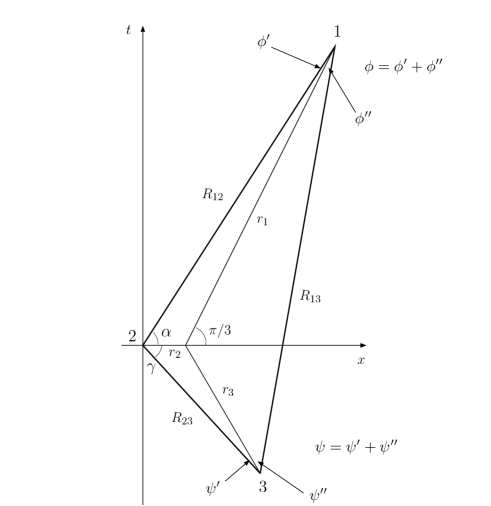
Figure 1: Triangle associated to the three-point correlation function. The orientation of the triangle has been chosen so that one of the three segments joining the vertices with the Steiner point lies on the real axis.

Then, taking into account that the residue on the bound state gives the condition

$$-i\;\textrm{Res}_{\theta_{-}=\frac{2\pi i}{3}-i\alpha_{+}}F_{AA}^{\sigma}(\theta_{-}+i\alpha_{+})=\Gamma^{\bar{A}}_{AA}F_{\bar{A}}^{\sigma}$$

($\alpha_{+}=\alpha+\gamma$) and using the Cauchy’s theorem (see Appendix A for details), we can write $G^{(3)}_{[1,1]}$ as follows

$$G^{(3)}_{[1,1]}(x_{1},x_{2},x_{3})=H\left(\frac{2\pi}{3}-\alpha_{+}\right)\;\frac{(F_{\bar{A}}^{\sigma})^{3}\;\Gamma^{\bar{A}}_{AA}}{\pi}K_{0}(mr_{Y})+$$ (31)

$$+(F_{\bar{A}}^{\sigma})^{2}\int_{-\infty}^{\infty}\frac{\textrm{d}\beta}{2\pi}\int_{-\infty}^{\infty}\frac{\textrm{d}\theta}{2\pi}F_{AA}^{\sigma}(\beta-\theta+i(\alpha+\gamma))\exp\left[-m\left(R_{12}\cosh\beta+R_{23}\cosh\theta\right)\right].$$

where $H(z)$ is the usual step-function and $r_{Y}=\sum_{i=1}^{3}r_{i}$ (see fig. 1)

3.4 $[1,2]$ & $[2,1]$ contributions

According to the general formula, the next-to-leading term of the spectral series is given by

$$G^{(3)}_{2p}(x_{1},x_{2},x_{3})\ =\ G^{(3)}_{[1,2]}(x_{1},x_{2},x_{3})+G^{(3)}_{[2,1]}(x_{1},x_{2},x_{3})=$$

$$=\frac{1}{2!}\int_{-\infty}^{\infty}\frac{\textrm{d}\beta}{2\pi}\int_{-\infty}^{\infty}\frac{\textrm{d}\theta_{1}\textrm{d}\theta_{2}}{(2\pi)^{2}}\langle 0|\sigma(x_{1})|\bar{A}(\beta)\rangle\langle{\bar{A}}(\beta)|\sigma(x_{2})|{\bar{A}}(\theta_{1}){\bar{A}}(\theta_{2})\rangle\langle{\bar{A}}(\theta_{2}){\bar{A}}(\theta_{1})|\sigma(x_{3})|0\rangle+$$

$$+\frac{1}{2!}\int_{-\infty}^{\infty}\frac{\textrm{d}\beta}{2\pi}\int_{-\infty}^{\infty}\frac{\textrm{d}\theta_{1}\textrm{d}\theta_{2}}{(2\pi)^{2}}\langle 0|\sigma(x_{1})|A(\theta_{1})A(\theta_{2})\rangle\langle A(\theta_{2})A(\theta_{1})|\sigma(x_{2})|A(\beta)\rangle\langle A(\beta)|\sigma(x_{3})|0\rangle$$

and hence, extracting the space-time dependence of the matrix elements, we obtain

$$G^{(3)}_{2p}(x_{1},x_{2},x_{3})\ =\ G^{(3)}_{[1,2]}(x_{1},x_{2},x_{3})+G^{(3)}_{[2,1]}(x_{1},x_{2},x_{3})=$$ (32)

$$=\frac{1}{2!}\int_{-\infty}^{\infty}\frac{\textrm{d}\beta}{2\pi}\int_{-\infty}^{\infty}\frac{\textrm{d}\theta_{1}\textrm{d}\theta_{2}}{(2\pi)^{2}}\langle 0|\sigma(0)|\bar{A}(\beta)\rangle\langle{\bar{A}}(\beta)|\sigma(0)|{\bar{A}}(\theta_{1}){\bar{A}}(\theta_{2})\rangle\langle{\bar{A}}(\theta_{2}){\bar{A}}(\theta_{1})|\sigma(0)|0\rangle\times$$

$$\hskip 8.5359pt\exp\left[-im\left(R_{12}\sinh(\beta-i\alpha)-R_{23}(\sinh(\theta_{1}+i\gamma)+\sinh(\theta_{2}+i\gamma))\right)\right]+$$

$$+\frac{1}{2!}\int_{-\infty}^{\infty}\frac{\textrm{d}\beta}{2\pi}\int_{-\infty}^{\infty}\frac{\textrm{d}\theta_{1}\textrm{d}\theta_{2}}{(2\pi)^{2}}\langle 0|\sigma(0)|A(\theta_{1})A(\theta_{2})\rangle\langle A(\theta_{2})A(\theta_{1})|\sigma(0)|A(\beta)\rangle\langle A(\beta)|\sigma(0)|0\rangle\times$$

$$\exp\left[-im\left(R_{12}(\sinh(\theta_{1}-i\alpha)+\sinh(\theta_{2}-i\alpha))-R_{23}\sinh(\beta+i\gamma)\right)\right].$$

It turns out that the above term gives a contribution to the correlator of the same order of magnitude of $G^{(3)}_{[1,1]}$. In order to understand this let us first notice that the matrix elements have to be rewritten in terms of form factors (which are the quantities that one actually computes in integrable field theories). Such a reduction to form factors is achieved by iterating the crossing relation [12, 13, 20], and in the case of $G^{(3)}_{[1,2]}$ (the treatment of $G^{(3)}_{[2,1]}$ will follow the same guidelines) we have

$$\langle{\bar{A}}(\beta)|\sigma(0)|{\bar{A}}(\theta_{1}){\bar{A}}(\theta_{2})\rangle=\ \langle 0|\sigma(0)|A(\beta+i\pi){\bar{A}}(\theta_{1}){\bar{A}}(\theta_{2})\rangle+$$

$$+2\pi\delta(\beta-\theta_{1})\langle 0|\sigma(0)|\bar{A}(\beta)\rangle+2\pi\delta(\beta-\theta_{2})u(\theta_{1}-\beta)\langle 0|\sigma(0)|\bar{A}(\beta)\rangle=$$

$$=F^{\sigma}_{A{\bar{A}}{\bar{A}}}(\beta+i\pi,\theta_{1},\theta_{2})+2\pi(\delta(\beta-\theta_{1})+\delta(\beta-\theta_{2})u(\theta_{1}-\beta))F^{\sigma}_{{\bar{A}}}\,.$$

Plugging the previous expression in $G^{(3)}_{[1,2]}$ and performing the integration over the delta functions, we obtain

$$G^{(3)}_{[1,2]}(x_{1},x_{2},x_{3})= \frac{F^{\sigma}_{\bar{A}}}{2!}\int_{-\infty}^{\infty}\frac{\textrm{d}\beta}{2\pi}\int_{-\infty}^{\infty}\frac{\textrm{d}\theta_{1}\textrm{d}\theta_{2}}{(2\pi)^{2}}F^{\sigma}_{A{\bar{A}}{\bar{A}}}(\beta+i\pi,\theta_{1},\theta_{2})F^{\sigma}_{AA}(\theta_{2}-\theta_{1})\times$$

$$\hskip 8.5359pt\exp\left[-im\left(R_{12}\sinh(\beta-i\alpha)-R_{23}(\sinh(\theta_{1}+i\gamma)+\sinh(\theta_{2}+i\gamma))\right)\right]+$$

$$+\frac{(F^{\sigma}_{\bar{A}})^{2}}{2!}\int_{-\infty}^{\infty}\frac{\textrm{d}\theta_{1}\textrm{d}\theta_{2}}{(2\pi)^{2}}F^{\sigma}_{AA}(\theta_{2}-\theta_{1})\exp\left[-im\left(R_{12}\sinh(\theta_{1}-i\alpha)-R_{23}(\sinh(\theta_{1}+i\gamma)+\sinh(\theta_{2}+i\gamma))\right)\right]+$$

$$+\frac{(F^{\sigma}_{\bar{A}})^{2}}{2!}\int_{-\infty}^{\infty}\frac{\textrm{d}\theta_{1}\textrm{d}\theta_{2}}{(2\pi)^{2}}F^{\sigma}_{AA}(\theta_{1}-\theta_{2})\exp\left[-im\left(R_{12}\sinh(\theta_{2}-i\alpha)-R_{23}(\sinh(\theta_{1}+i\gamma)+\sinh(\theta_{2}+i\gamma))\right)\right]$$

where in the last line we have used the fact that $F^{\sigma}_{AA}(\theta)=u(\theta)F^{\sigma}_{AA}(-\theta)$. A brief inspection of such an expression shows that the last two terms coincide (to see this one can make the exchange $\theta_{1}\leftrightarrow\theta_{2}$ in one of them), and hence we can write

$$G^{(3)}_{[1,2]}(x_{1},x_{2},x_{3})= \frac{F^{\sigma}_{\bar{A}}}{2!}\int_{-\infty}^{\infty}\frac{\textrm{d}\beta}{2\pi}\int_{-\infty}^{\infty}\frac{\textrm{d}\theta_{1}\textrm{d}\theta_{2}}{(2\pi)^{2}}F^{\sigma}_{A{\bar{A}}{\bar{A}}}(\beta+i\pi,\theta_{1},\theta_{2})F^{\sigma}_{AA}(\theta_{2}-\theta_{1})\times$$

$$\hskip 8.5359pt\exp\left[-im\left(R_{12}\sinh(\beta-i\alpha)-R_{23}(\sinh(\theta_{1}+i\gamma)+\sinh(\theta_{2}+i\gamma))\right)\right]+$$

$$+\ (F^{\sigma}_{\bar{A}})^{2}\int_{-\infty}^{\infty}\frac{\textrm{d}\theta_{1}\textrm{d}\theta_{2}}{(2\pi)^{2}}F^{\sigma}_{AA}(\theta_{2}-\theta_{1})\exp\left[-im\left(R_{12}\sinh(\theta_{1}-i\alpha)-R_{23}(\sinh(\theta_{1}+i\gamma)+\sinh(\theta_{2}+i\gamma))\right)\right].$$

Such an expression for $G^{(3)}_{[1,2]}$ shows that the disconnected parts sum up giving a contribution which is quite similar to $G^{(3)}_{[1,1]}$. Hence, if we pose

$$G^{(3),disc}_{[1,2]}(x_{1},x_{2},x_{3})= \ (F^{\sigma}_{\bar{A}})^{2}\,\int_{-\infty}^{\infty}\frac{\textrm{d}\theta_{1}\textrm{d}\theta_{2}}{(2\pi)^{2}}F^{\sigma}_{AA}(\theta_{2}-\theta_{1})\times$$

$$\hskip 8.5359pt\exp\left[-im\left(R_{12}\sinh(\theta_{1}-i\alpha)-R_{23}(\sinh(\theta_{1}+i\gamma)+\sinh(\theta_{2}+i\gamma))\right)\right]$$

and we use the Cauchy’s theorem taking into account the residue condition on the bound state, we obtain (see Appendix A for details)

$$G^{(3),disc}_{[1,2]}(x_{1},x_{2},x_{3})\ =\ -H\left(\psi-\frac{2\pi}{3}\right)\;\frac{(F_{\bar{A}}^{\sigma})^{3}\;\Gamma^{\bar{A}}_{AA}}{\pi}K_{0}(mr_{Y})+$$

$$+(F_{\bar{A}}^{\sigma})^{2}\int_{-\infty}^{\infty}\frac{\textrm{d}\theta_{1}\textrm{d}\theta_{2}}{(2\pi)^{2}}F_{AA}^{\sigma}(\theta_{2}-\theta_{1}+i\psi)\exp\left[-m\left(R_{23}\cosh\theta_{2}+R_{13}\cosh\theta_{1}\right)\right].$$

One can notice the change of sign in front of the function $H(z)$ and the difference in its argument with respect to $G^{(3)}_{[1,1]}$.

As anticipated, we can treat $G^{(3)}_{[2,1]}$ in exactly the same way as $G^{(3)}_{[1,2]}$. At the end of the computation we are left with the following expression for $G^{(3),disc}_{[2,1]}$

$$G^{(3),disc}_{[2,1]}(x_{1},x_{2},x_{3})\ =\ -H\left(\phi-\frac{2\pi}{3}\right)\;\frac{(F_{\bar{A}}^{\sigma})^{3}\;\Gamma^{\bar{A}}_{AA}}{\pi}K_{0}(mr_{Y})+$$

$$+(F_{\bar{A}}^{\sigma})^{2}\int_{-\infty}^{\infty}\frac{\textrm{d}\theta_{1}\textrm{d}\theta_{2}}{(2\pi)^{2}}F_{AA}^{\sigma}(\theta_{1}-\theta_{2}+i\phi)\exp\left[-m\left(R_{13}\cosh\theta_{1}+R_{12}\cosh\theta_{2}\right)\right].$$

Collecting all the previous contributions we can write down the explicit expression of the spectral series for the three-point function up to one-particle contributions

$$G^{(3)}(x_{1},x_{2},x_{3})\ =\ G^{(3)}_{[1,1]}+G^{(3),disc}_{[1,2]}+G^{(3),disc}_{[2,1]}+\dots=$$ (39)

$$=\left\{H\left(\frac{2\pi}{3}-\alpha_{+}\right)-H\left(\psi-\frac{2\pi}{3}\right)-H\left(\phi-\frac{2\pi}{3}\right)\right\}\;\frac{(F_{\bar{A}}^{\sigma})^{3}\;\Gamma^{\bar{A}}_{AA}}{\pi}K_{0}(mr_{Y})+$$

$$+(F_{\bar{A}}^{\sigma})^{2}\int_{-\infty}^{\infty}\frac{\textrm{d}\beta\textrm{d}\theta}{(2\pi)^{2}}F_{AA}^{\sigma}(\beta-\theta+i\alpha_{+})\exp\left[-m\left(R_{12}\cosh\beta+R_{23}\cosh\theta\right)\right]+$$

$$+F_{AA}^{\sigma}(\beta-\theta+i\psi)\exp\left[-m\left(R_{23}\cosh\beta+R_{13}\cosh\theta\right)\right]+$$

$$+F_{AA}^{\sigma}(\beta-\theta+i\phi)\exp\left[-m\left(R_{13}\cosh\beta+R_{12}\cosh\theta\right)\right]+\dots.$$

Some comments about the previous expression are in order.

• The combination of $H(z)$ functions which appears in the first term nicely realizes the condition stated at the beginning of the section. It is not difficult to show that only two possibilities are allowed: either all the angles are less than $2\pi/3$ and such a prefactor is 1, or one of them is larger than $2\pi/3$ and then the prefactor is zero.

• The second term of (39) shows explicitly that its asymptotic behaviour for large distances is given by $O(e^{-m\rho})$ where

  $$\rho=\min(R_{12}+R_{23},R_{23}+R_{31},R_{12}+R_{31}).$$

3.5 Isosceles & Equilateral triangles

Formula (39) can be simplified by means of a wise choice of the geometry of the triangle.

Let us begin with the case of isosceles triangles. We decide to make the choice: $R=R_{12}=R_{23}$, $S=R_{13}=2R\sin\alpha$, and $\alpha=\gamma$ ($\alpha_{+}=2\alpha$), $\psi=\phi=\pi/2-\alpha$ (it is easy to show that any other choice of the isosceles triangle will be equivalent to the previous one). Hence (39) will take the following form

$$G^{(3)}(x_{1},x_{2},x_{3})\ \simeq\ H\left(\frac{\pi}{3}-\alpha\right)\;\frac{(F_{\bar{A}}^{\sigma})^{3}\;\Gamma^{\bar{A}}_{AA}}{\pi}K_{0}\left(2mR\cos\left(\frac{\pi}{3}-\alpha\right)\right)+$$

$$+2(F_{\bar{A}}^{\sigma})^{2}\int_{-\infty}^{\infty}\frac{\textrm{d}\theta}{(2\pi)^{2}}F_{AA}^{\sigma}(\theta+2i\alpha)K_{0}\left(2mR\cosh\frac{\theta}{2}\right)+$$

$$+2(F_{\bar{A}}^{\sigma})^{2}\int_{-\infty}^{\infty}\frac{\textrm{d}\beta\textrm{d}\theta}{(2\pi)^{2}}F_{AA}^{\sigma}(\beta-\theta+i(\pi/2-\alpha))\exp\left[-mR\left(\cosh\beta+2\sin\alpha\cosh\theta\right)\right]\,.$$

An even simpler form can be found when the case of equilateral triangles is considered. Such a choice corresponds to fixing $\alpha=\pi/6$ in the previous formula (obviously one can obtain the same result directly from formula (39)) finding

$$G^{(3)}(x_{1},x_{2},x_{3})\ \simeq\ \frac{(F_{\bar{A}}^{\sigma})^{3}\;\Gamma^{\bar{A}}_{AA}}{\pi}K_{0}\left(\sqrt{3}\,mR\right)+$$ (40)

$$+\ 6(F_{\bar{A}}^{\sigma})^{2}\int_{-\infty}^{\infty}\frac{\textrm{d}\theta}{(2\pi)^{2}}F_{AA}^{\sigma}(\theta+i\pi/3)K_{0}\left(2mR\cosh\frac{\theta}{2}\right).$$

4 Monte-Carlo simulations

We performed Monte-Carlo simulations of the 3-state Potts model on a triangular lattice (where each site has six nearest neighbors, see fig. 2) with honeycomb boundary conditions. This lattice has a larger symmetry than a square lattice and allowed us to study 3-point functions with three exactly equidistant points. A Swendsen-Wang cluster algorithm was used and 2- and 3-point functions were computed from improved estimators. The latter proved essential for the 3-point function, which could not have been measured to as large distances with conventional estimators. Simulations were performed at three different couplings, see table 1 below. In the table, a volume $60\times 180$, for instance, refers to a hexagon with side $60$.

Figure 2: Triangular lattice.

4.1 Determination of the mass and $F^{\sigma}_{\bar{A}}$

The long-distance expansion for the 2-point function has two free parameters, the mass (inverse correlation length) and the 1-particle form factor. For each lattice, the mass was extracted from the effective mass, defined in terms of the wall-wall correlator $G^{\ell}_{0}(x)$ as

$$m_{\text{eff}}(x+\tfrac{1}{4})\equiv 2\ln\frac{G^{\ell}_{0}(x)}{G^{\ell}_{0}(x+\tfrac{1}{2})}$$ (41)

On a triangular lattice,

$$G^{\ell}_{0}(x)=\sum_{y}\langle\sigma_{\ell}(x,y)\bar{\sigma}_{\ell}(0,0)\rangle\simeq\frac{1}{\sqrt{3}}\int{\mathrm{d}}y\,\langle\sigma_{\ell}(x,y)\bar{\sigma}_{\ell}(0,0)\rangle$$ (42)

where the factor $1/\sqrt{3}$ comes from the distance between points along the wall on a triangular lattice, see fig. 2. Note also that a displacement of $\tfrac{1}{2}$ instead of $1$ is possible on such a lattice.

The prediction of 1- and 2-particle contributions for the propagator including finite-size effects for the 1-particle contribution (those from the 2-particle contribution are negligible) is

$$G^{\ell}_{0}(x)=\frac{(F_{\ell})^{2}}{\sqrt{3}m}\left({\mathrm{e}}^{-mx}+g_{2}(mx)+{\mathrm{e}}^{-m(L-x)}\right)$$ (43)

where

$$g_{2}(mx)=\frac{1}{2\pi}\int_{0}^{\infty}{\mathrm{d}}\theta\left|\frac{F^{\sigma}_{AA}(2\theta)}{F^{\sigma}_{\bar{A}}}\right|^{2}\frac{\exp[-2mx\cosh\theta]}{\cosh\theta}$$ (44)

and $F_{\ell}$ is the 1-particle form factor $F^{\sigma}_{\bar{A}}$ in lattice normalization. The corresponding effective mass is

$$m_{\text{eff}}(x+\tfrac{1}{4})=m+\delta m_{\text{eff}}(x+\tfrac{1}{4},m,L)$$ (45)

with

$$\delta m_{\text{eff}}(x+\tfrac{1}{4},m,L)=2\ln\frac{1+{\mathrm{e}}^{mx}g_{2}(mx)+{\mathrm{e}}^{-m(L-2x)}}{1+{\mathrm{e}}^{m(x+1/2)}g_{2}(m(x+\tfrac{1}{2}))+{\mathrm{e}}^{-m(L-2x-1)}}$$ (46)

The fit with this function is performed by subtracting $\delta m_{\text{eff}}(x,m,L)$ with some trial $m$ from the effective mass data, fitting the result to a constant, and then iteratively improving $m$. This procedure is very stable because the corrections are small in the range of the fit. The fit at $\beta=0.613$ is shown in fig. 3. It confirms the analytic prediction very well. The resulting masses and correlation lengths, together with the fit ranges used, can be found in table 1. The error estimates were obtained with a jackknife analysis.

$\beta$	volume	$\xi$	$m$	$F_{\ell}$	$x_{\text{min}}$	$x_{\text{max}}$	$\Gamma^{\bar{A}}_{AA}$
0.5900	$60\times 180$	$4.5184(9)$	$0.22132(5)$	$0.92179(19)$	$7.5$	$25$	$1.2609(16)$
0.6130	$120\times 360$	$9.093(3)$	$0.10997(3)$	$0.8233(2)$	$15$	$50$	$1.287(3)$
0.6231	$240\times 720$	$18.232(7)$	$0.054849(19)$	$0.7420(3)$	$25$	$125$	$1.299(3)$

Table 1: Simulation parameters.

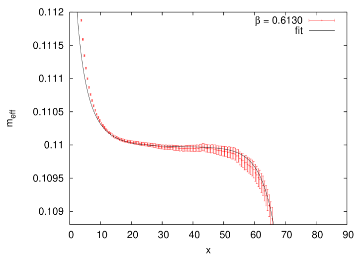
Figure 3: Effective mass at $\beta=0.613$ and 1-parameter fit from eq. (45) including the long-distance expansion up to 2 particles and finite-size effects. $x$ has period 180.

Given the mass, the 1-particle form factor can be obtained from the wall-wall correlator by fitting the prefactor in (43). The result at $\beta=0.613$ is shown in fig. 4. The long-distance expansion and finite-size effects describe the data very well. The resulting 1-particle form factors are given in table 1. The error estimates were again obtained from a jackknife analysis which also included the determination of the mass described above.

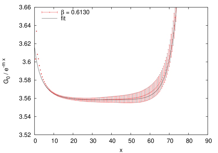
Figure 4: Wall-wall correlator at $\beta=0.613$ and 2-particle prediction with finite-size effects. Only the prefactor has been fitted.

The long-distance expansion of the 2-point function is completely determined by $m$ and $F_{\ell}$. Figure 5 shows the 2-point function divided by the 1-particle term of the long-distance expansion and rescaled by $m$ and $F_{\ell}$. The data from the three different lattices collaps nicely, and the small deviations from the 1-particle term are well described by the 2-particle term.

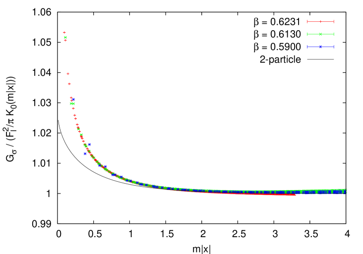
Figure 5: Two-point function, rescaled using $m$ and $F_{\ell}$ from fits to the wall-wall correlator and divided by 1-particle term of long-distance expansion.

4.2 Scaling violations

Comparing the results from the different lattices, we may estimate the size of the scaling violations which we must expect in our results.

Setting

$$t\equiv\frac{T-T_{c}}{T_{c}}=\frac{\beta_{c}-\beta}{\beta}$$ (47)

we expect $m\sim t^{5/6}$ and $F_{\ell}\sim t^{1/9}$. Figures 6 and 7 show the ratios $m/t^{5/6}$ and $F_{\ell}/t^{1/9}$ as a function of $t$. They vary by about $3\%$, a reasonable size for scaling violations at these correlation lengths.

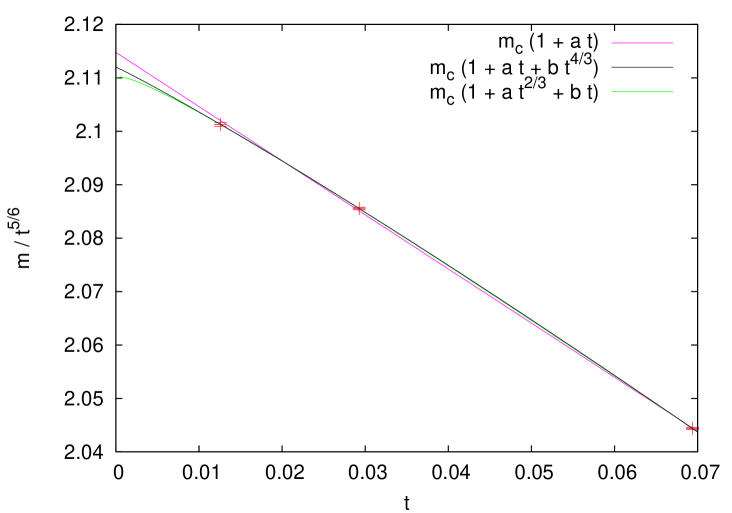
Figure 6: Correction to scaling for $m$.

Figure 7: Correction to scaling for $F_{\ell}$.

The scaling violations in the mass are expected to be of the form

$$m(t)/t^{5/6} =m_{c}(1+a_{m,\Delta}t^{\Delta}+a_{m,1}t+\dots)\,.$$ (48)

Taking into account that the subleading thermal operator $\epsilon^{\prime}$ corresponds to the conformal operator $(3,1;3,1)$, the leading correction-to-scaling exponent is $\Delta=-\frac{2-X_{\epsilon^{\prime}}}{2-X_{\epsilon}}=\frac{2}{3}$. This value has been first determined in [21] and later confirmed in [22, 23, 24], see [25]. We find $a_{m,\Delta}\ll a_{m,1}$. A fit with only one term and variable exponent $p$ yields $p=1.10\dots$. These two facts indicate that $a_{m,\Delta}$ may vanish. A fit with only the linear term has $\chi^{2}=7.7$, so we perform a fit with the next two terms,

$$m_{c}(1+a_{m,1}t+a_{m,2\Delta}t^{2\Delta})\;.$$ (49)

Since it has as many parameters as data points, we use the fit with only the linear term for an error estimate. The result is

$$m_{c}=2.112(3)\;.$$ (50)

The statistical error from the fit with only a linear term is much smaller. The fits are shown in fig. 6.

For $F_{\ell}$, a fit to

$$F_{\ell}(t)/t^{1/9} =F_{c}(1+a_{F,\Delta}t^{\Delta}+a_{F,1}t+\dots)$$ (51)

yields a linear term which is much smaller than the leading correction. We use a fit with only the leading correction for an error estimate and obtain

$$F_{c}=1.189(3)\;.$$ (52)

Again the statistical errors from the latter fit are smaller than the quoted error. Both fits are shown in fig. 7.

4.3 3-point function

The long-distance expansion of the 3-point function is completely determined by $m$ and $F_{\ell}$. In particular, $G_{\ell}^{(3)}/F_{\ell}^{3}$ as a function of $mx_{i}$ is independent of any parameters. The measured 3-point functions, rescaled in this way, are shown in fig. 8. Also shown is the long-distance expansion of eq. (40) which we split into “Y-type” and “$\Lambda$-type” contributions (the second term depends on sums of two spin–spin-distances),

$$G_{\ell}^{(3)}(x_{1},x_{2},x_{3})=F_{\ell}^{3}\Gamma^{\bar{A}}_{AA}\bigl{[}g_{\textrm{Y}}(x_{1},x_{2},x_{3})+g_{\Lambda}(x_{1},x_{2},x_{3})\bigr{]}$$ (53)

with

$$g_{\textrm{Y}}(x_{1},x_{2},x_{3}) =\frac{1}{\pi}K_{0}(mr_{Y})$$ (54)

$$g_{\Lambda}(x_{1},x_{2},x_{3}) =\frac{3}{2\pi^{2}}\int_{-\infty}^{\infty}{\mathrm{d}}\theta\,\frac{F^{\sigma}_{AA}(\theta+{\mathrm{i}}\pi/3)}{F^{\sigma}_{\bar{A}}\Gamma^{\bar{A}}_{AA}}K_{0}\left(2mR\cosh\frac{\theta}{2}\right)$$ (55)

where $R=|x_{1}-x_{2}|=|x_{2}-x_{3}|=|x_{3}-x_{1}|$ is the distance between two spins and $r_{Y}=\sqrt{3}R$ the Y-length. For the equilateral geometry, the Y-type term is leading. It is shown separately in the figure. The subleading $\Lambda$-type term is sizable up to large distances. This is not unexpected as the sum of two sides, $2R$, is only 15% larger than the Y length $\sqrt{3}R$.

Figure 8: Three-point function, rescaled using $m$ and $F_{\ell}$ from fits to the wall-wall correlator.

The deviation from the leading Y-type term is shown in fig. 9. Scaling violations are clearly visible and turn out to be of the same order as those observed in the 2-point function, i.e. about $3\%$. These scaling violations have to be expected (even after rescaling with $m$ and $F_{\ell}$) since the lattice model at a given temperature $t$ is effectively described by a quantum field theory which differs from the scaling theory (6) by irrelevant operators. The form factors therefore differ from the values computed exactly in the integrable scaling theory. The two terms above contain the three-particle coupling constant $\Gamma^{\bar{A}}_{AA}$ and the 2-particle form factor $F^{\sigma}_{AA}(\theta)$ which is also proportional to $\Gamma^{\bar{A}}_{AA}$. Lacking an understanding of the rapidity-dependence of the scaling violations, we proceed by ignoring all scale-dependence in $F^{\sigma}_{AA}$ other than that induced by $\Gamma^{\bar{A}}_{AA}$, i.e. we replace the prefactor $\Gamma^{\bar{A}}_{AA}$ in (53) by a function of $t$. This works very well, as can be seen from the figure. The remaining deviations may well be due to higher-order terms in the long-distance expansion. The resulting values for the three-particle coupling are given in table 1. The quoted errors were taken from the 3-point function at distances where $G_{\ell}^{(3)}/(g_{Y}+g_{\Lambda})$ approaches a constant. They are therefore only rough estimates. The values of $\Gamma^{\bar{A}}_{AA}(t)$ nicely approach the value $3^{1/4}=1.316\dots$ in the scaling theory. The corresponding curve is also shown in the figure. Note that this curve does not depend on any fits, but is completely determined by the values of $m$ and $F_{\ell}$ extracted from the wall-wall correlator.

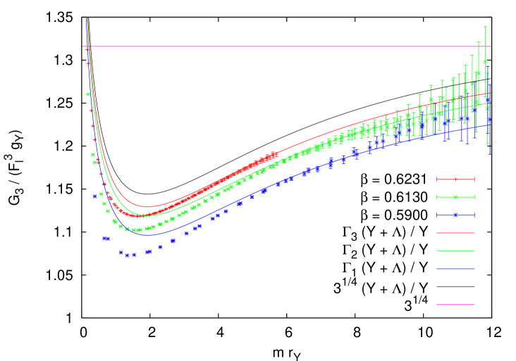
Figure 9: Same as fig. 8, but divided by the leading (Y-type) contribution. Note the larger range.

5 Short distance expansion

5.1 2-point function

In order to have good control on the $\langle\sigma\bar{\sigma}\rangle$ correlation function it is worth to compare the Monte-Carlo data in the short distance regime with the corresponding perturbative expansion obtained in the framework of the so-called Conformal Perturbation Theory. Since such a perturbative expansion is expected to be valid in the region $m|x|\ll 1$, it is a complementary tool with respect to the form factor expansion discussed before.

Let us recall the main results about Conformal Perturbation Theory in the special case of the correlation function $\langle\sigma(x){\bar{\sigma}}(0)\rangle$. Following the standard literature on the subject [26]-[29] we may write such a correlator as

$$G_{\sigma}(x)=\langle\sigma(x){\bar{\sigma}}(0)\rangle=\sum_{p}{\mathcal{C}}_{\sigma{\bar{\sigma}}}^{[\phi_{p}]}(x;\tau)\langle[\phi_{p}]\rangle$$ (56)

here the sum over $p$ ranges over all the conformal families allowed by the Operator Product Expansion of $\sigma$ and $\bar{\sigma}$. The Wilson coefficients ${\mathcal{C}}_{\sigma{\bar{\sigma}}}^{[\phi_{p}]}$ can be calculated perturbatively in the coupling constant $\tau$. Their Taylor expansion (w.r.t. $\tau$) is:

$${\mathcal{C}}_{\sigma{\bar{\sigma}}}^{[\phi_{p}]}(x;\tau)=\sum_{k}\frac{\tau^{k}}{k!}\partial^{k}_{\tau}{\mathcal{C}}_{\sigma{\bar{\sigma}}}^{[\phi_{p}]}(x;0).$$ (57)

It is possible to show that the derivatives of the Wilson coefficients which appear in the previous expression can be written in terms of multiple integrals of the conformal correlators

$$\partial^{k}_{\tau}{\mathcal{C}}_{\sigma{\bar{\sigma}}}^{[\phi_{p}]}(x;0)=(-1)^{k}\int^{{}^{\prime}}d^{2}z_{1}\dots d^{2}z_{k}\,\langle\sigma(x){\bar{\sigma}(0)}\epsilon(z_{1})\dots\epsilon(z_{k})[\phi_{p}](\infty)\rangle_{\textrm{\tiny cft}}$$ (58)

where the prime on the integral implies a suitable treatment of the IR divergences and we used a shorthand notation to denote the follwoing limit:

$$\langle\sigma(x_{1}).....\epsilon(\infty)\rangle_{\textrm{\tiny cft}}=\lim_{w\to\infty}\frac{\langle\sigma(x_{1}).....\epsilon(w)\rangle_{\textrm{\tiny cft}}}{\langle\epsilon(w)\epsilon(0)\rangle_{\textrm{\tiny cft}}}~{}~{}~{}.$$ (59)

For all the details we address the interested reader to the original literature [27].

Another important piece of information which enters the perturbative expansion of the correlator is represented by the Vacuum Expectation Values $\langle[\phi_{p}]\rangle$. Such VEVs cannot be calculated in the framework of the perturbation theory, and being non-perturbative objects they have to be obtained by other methods. By using the powerful techniques of Integrable QFTs, they were computed in a series of papers [30]-[32] for a wide class of theories, including various integrable perturbations of the Minimal Models.

The leading term of the perturbative expansion is given by the 2-point conformal correlator which corresponds to the choice $k=0$ and $\phi_{p}=\mathbb{I}$

$${\mathcal{C}}_{\sigma{\bar{\sigma}}}^{\mathbb{I}}(x;0)=\frac{1}{|x|^{4/15}}$$ (60)

which follows from the choice of the conformal normalization $C_{\sigma{\bar{\sigma}}}^{\mathbb{I}}=1$.

The first few sub-leading terms are

$$G_{\sigma}(x)=\langle\sigma(x){\bar{\sigma}}(0)\rangle={\mathcal{C}}_{\sigma{\bar{\sigma}}}^{\mathbb{I}}(x;\tau)+{\mathcal{C}}_{\sigma{\bar{\sigma}}}^{\epsilon}(x;\tau)\langle\epsilon\rangle+\dots$$ (61)

where

$${\mathcal{C}}_{\sigma{\bar{\sigma}}}^{\mathbb{I}}(x;\tau) = {\mathcal{C}}_{\sigma{\bar{\sigma}}}^{\mathbb{I}}(x;0)+\tau\,\partial_{\tau}{\mathcal{C}}_{\sigma{\bar{\sigma}}}^{\mathbb{I}}(x;0)+\dots$$

$${\mathcal{C}}_{\sigma{\bar{\sigma}}}^{\epsilon}(x;\tau) = {\mathcal{C}}_{\sigma{\bar{\sigma}}}^{\epsilon}(x;0)+\dots,$$ (62)

give corrections up to $\tau$. The explicit expression of the various contributions is, together with (60),

$$\partial_{\tau}{\mathcal{C}}_{\sigma{\bar{\sigma}}}^{\mathbb{I}}(x;0) = -\int d^{2}z\langle\sigma(x){\bar{\sigma}(0)}\epsilon(z)\rangle_{\textrm{\tiny cft}}=-C_{\sigma{\bar{\sigma}}}^{\epsilon}\,|x|^{14/15}\int d^{2}y|y|^{-4/5}|1-y|^{-4/5}$$

$$= \sin\frac{4\pi}{5}\left|\frac{\Gamma(-1/5)\Gamma(3/5)}{\Gamma(2/5)}\right|^{2}C_{\sigma{\bar{\sigma}}}^{\epsilon}\,|x|^{14/15}$$

$${\mathcal{C}}_{\sigma{\bar{\sigma}}}^{\epsilon}(x;0) = C_{\sigma{\bar{\sigma}}}^{\epsilon}\,|x|^{8/15}$$ (63)

where the Wilson coefficient

$$C_{\sigma{\bar{\sigma}}}^{\epsilon} = \frac{1}{2}\sqrt{\frac{\sin\frac{2\pi}{5}}{\sin\frac{\pi}{5}}}\,\frac{\Gamma^{2}(3/5)}{\Gamma(2/5)\Gamma(4/5)}=0.546178\dots$$ (64)

can be found combining the results of [33] and [34] (see also [35]). The integral which appears in $\partial_{\tau}{\mathcal{C}}_{\sigma{\bar{\sigma}}}^{\mathbb{I}}(x;0)$ is well known. It is a particular case of the following one

$${\mathcal{Y}}_{a,b}=\int d^{2}z|z|^{2a}|1-z|^{2b}=\frac{\sin\pi(a+b)\,\sin\pi b}{\sin\pi a}\left|\frac{\Gamma(-a-b-1)\Gamma(b+1)}{\Gamma(-a)}\right|^{2}~{}~{}~{}~{}.$$ (65)

Its value is: ${\mathcal{Y}}_{-\frac{2}{5},-\frac{2}{5}}=-8.97743\dots$.

At last, let us discuss the other (non-perturbative) quantities we need: the VEV of the perturbing operator $\epsilon(x)$ and the relation between the coupling constant and the mass of the fundamental particle. The latter is known, and can be extracted from [36]

$$\tau=\kappa\,m^{6/5},\ \ \ \ \kappa=0.164303\dots.$$ (66)

The VEV $\langle\epsilon\rangle$ can be easily computed starting from the knowledge of the vacuum energy density [37]

$$\varepsilon_{0}=-\frac{\sqrt{3}}{6}m^{2}$$ (67)

which is related to the VEV of the perturbing operator by means of the relation

$$\langle\epsilon\rangle=\partial_{\tau}\varepsilon_{0}=A_{\epsilon}\,\tau^{2/3}=-9.761465\dots\tau^{2/3}=-2.92827\dots m^{4/5}.$$ (68)

Collecting the above ingredients, the perturbative series can be cast in the following form

$$G_{\sigma}(x) = \frac{1}{|x|^{4/15}}\left(1+C_{\sigma{\bar{\sigma}}}^{\epsilon}A_{\epsilon}\,\tau^{2/3}|x|^{4/5}+{\mathcal{Y}}_{-\frac{2}{5},-\frac{2}{5}}C_{\sigma{\bar{\sigma}}}^{\epsilon}\,\tau|x|^{6/5}+\dots\right)$$

$$= \frac{1}{|x|^{4/15}}\left(1+C_{\sigma{\bar{\sigma}}}^{\epsilon}A_{\epsilon}\,u^{2/3}+{\mathcal{Y}}_{-\frac{2}{5},-\frac{2}{5}}C_{\sigma{\bar{\sigma}}}^{\epsilon}\,u+\dots\right)$$

$$= \frac{1}{|x|^{4/15}}\left(1+C_{\sigma{\bar{\sigma}}}^{\epsilon}A_{\epsilon}\kappa^{2/3}\,r^{4/5}+{\mathcal{Y}}_{-\frac{2}{5},-\frac{2}{5}}C_{\sigma{\bar{\sigma}}}^{\epsilon}\,\kappa\,r^{6/5}+\dots\right)$$

where we set $u=\tau|x|^{6/5}$, and $r=m|x|$, respectively.

5.2 3-point function

The perturbative approach of the previous section can be generalized to multipoint correlators as well. Following the guidelines of [29] one is able to write down a perturbative IR safe expansion

$$G^{(n)}(x)=\langle\phi_{1}(x_{1})\dots\phi_{n}(x_{n})\rangle=\sum_{p}{\mathcal{C}}_{\phi_{1}\dots\phi_{n}}^{[\phi_{p}]}(\underline{x};\tau)\langle[\phi_{p}]\rangle$$ (69)

where the structure functions ${\mathcal{C}}_{\phi_{1}\dots\phi_{n}}^{[\phi_{p}]}(\underline{x};\tau)$ are a generalization of those appearing in the formula for the two-point function. Their Taylor expansion gives

$${\mathcal{C}}_{\phi_{1}\dots\phi_{n}}^{[\phi_{p}]}(\underline{x};\tau)={\mathcal{C}}_{\phi_{1}\dots\phi_{n}}^{[\phi_{p}]}(\underline{x};0)+\sum_{\ell=1}^{\infty}\frac{\tau^{\ell}}{\ell!}\partial_{\tau}^{\ell}{\mathcal{C}}_{\phi_{1}\dots\phi_{n}}^{[\phi_{p}]}(\underline{x};0)$$ (70)

where we have

$${\mathcal{C}}_{\phi_{1}\dots\phi_{n}}^{[\phi_{p}]}(\underline{x};0)=\langle\phi_{1}(x_{1})\dots\phi_{n}(x_{n})[\phi_{p}](\infty)\rangle_{\textrm{\tiny cft}},$$ (71)

and

$$\partial_{\tau}^{\ell}{\mathcal{C}}_{\phi_{1}\dots\phi_{n}}^{[\phi_{p}]}(\underline{x};0)=(-1)^{\ell}\int^{{}^{\prime}}d^{2}z_{1}\dots d^{2}z_{\ell}\,\langle\phi_{1}(x_{1})\dots\phi_{n}(x_{n})\epsilon(z_{1})\dots\epsilon(z_{\ell})[\phi_{p}](\infty)\rangle_{\textrm{\tiny cft}}$$ (72)

where the operator $\epsilon(x)$ which appears in the previous expression is the perturbing operator conjugated to the coupling constant $\tau$.

In the present section we are interested in the 3-point function $G^{(3)}=\langle\sigma_{1}\sigma_{2}\sigma_{3}\rangle$, whose perturbative expression can be written according to the previous considerations as

$$G^{(3)}(x) = \langle\sigma(x_{1})\sigma(x_{2})\sigma(x_{3})\rangle=$$ (73)

$$= {\mathcal{C}}_{\sigma\sigma\sigma}^{{\mathbb{I}}}(x_{1},x_{2},x_{3};\tau)+{\mathcal{C}}_{\sigma\sigma\sigma}^{\epsilon}(x_{1},x_{2},x_{3};\tau)\,\langle\epsilon\rangle+\dots\,\,;$$

up to first order in $\tau$ one has

$${\mathcal{C}}_{\sigma\sigma\sigma}^{{\mathbb{I}}}(x_{1},x_{2},x_{3};\tau) = {\mathcal{C}}_{\sigma\sigma\sigma}^{{\mathbb{I}}}(x_{1},x_{2},x_{3};0)+\tau\,\partial_{\tau}{\mathcal{C}}_{\sigma\sigma\sigma}^{{\mathbb{I}}}(x_{1},x_{2},x_{3};0)+\dots$$

$${\mathcal{C}}_{\sigma\sigma\sigma}^{\epsilon}(x_{1},x_{2},x_{3};\tau) = {\mathcal{C}}_{\sigma\sigma\sigma}^{\epsilon}(x_{1},x_{2},x_{3};0)+\tau\,\partial_{\tau}{\mathcal{C}}_{\sigma\sigma\sigma}^{\epsilon}(x_{1},x_{2},x_{3};0)+\dots$$

The explicit expression of the zero-th order contributions can be derived quite easily. We have

$${\mathcal{C}}_{\sigma\sigma\sigma}^{{\mathbb{I}}}(x_{1},x_{2},x_{3};0) = \langle\sigma(x_{1})\sigma(x_{2})\sigma(x_{3})\rangle_{\textrm{\tiny cft}}=$$ (74)

$$= \frac{C^{\bar{\sigma}}_{\sigma\sigma}}{|x_{1}-x_{2}|^{2/15}|x_{2}-x_{3}|^{2/15}|x_{1}-x_{3}|^{2/15}}$$

where the structure constant $C^{\bar{\sigma}}_{\sigma\sigma}$ can be found in the literature [33, 34, 35]

$$C^{\bar{\sigma}}_{\sigma\sigma}=\sqrt{\frac{3\sin 2\pi/5}{\pi\sin\pi/5}}\frac{\Gamma(5/6)\Gamma^{2}(3/5)\Gamma^{4}(1/3)}{\Gamma(2/5)\Gamma(4/5)\Gamma^{2}(2/3)\Gamma^{2}(1/6)}=1.09236\dots.$$ (75)

The other zero-th order term is given by

$${\mathcal{C}}_{\sigma\sigma\sigma}^{\epsilon}(x_{1},x_{2},x_{3};0)=\langle\sigma(x_{1})\sigma(x_{2})\sigma(x_{3})\epsilon(\infty)\rangle_{\textrm{\tiny cft}}$$ (76)

whose main ingredient is the conformal four point correlator $\langle\sigma\sigma\sigma\epsilon\rangle$ which was computed in [41]. We consistently fixed its normalization constant, which gives

$$\langle\sigma(x_{1})\sigma(x_{2})\sigma(x_{3})\epsilon(x_{4})\rangle_{\textrm{\tiny cft}}=C^{\bar{\sigma}}_{\sigma\sigma}C^{\epsilon}_{\sigma{\bar{\sigma}}}\,\frac{|x_{12}x_{13}x_{23}|^{2/15}}{|x_{14}x_{24}x_{34}|^{8/15}}\,|y(1-y)|^{14/15}\,\left\{|f_{1}(y)|^{2}+K^{-1}|f_{2}(y)|^{2}\right\}$$ (77)

where

$$f_{1}(y)=y^{-3/5}{{}_{2}F_{1}}(1/5,4/5;2/5;y),\ \ \ f_{2}(y)={{}_{2}F_{1}}(4/5,7/5;8/5;y)$$ (78)

and

$$K=\frac{9\,\Gamma(1/5)\,\Gamma(3/5)^{3}}{4\,\Gamma(4/5)\,\Gamma(2/5)^{3}},\ \ \ y=\frac{x_{14}x_{23}}{x_{34}x_{21}},\ \ \ 1-y=\frac{x_{13}x_{24}}{x_{34}x_{12}}$$ (79)

Then, a simple computation gives

$${\mathcal{C}}_{\sigma\sigma\sigma}^{\epsilon}(x_{1},x_{2},x_{3};0)=C^{\bar{\sigma}}_{\sigma\sigma}C^{\epsilon}_{\sigma{\bar{\sigma}}}\,|x_{12}x_{13}x_{23}|^{2/15}|{\tilde{y}}(1-{\tilde{y}})|^{14/15}\,\left\{|f_{1}({\tilde{y}})|^{2}+K^{-1}|f_{2}({\tilde{y}})|^{2}\right\}$$ (80)

where

$${\tilde{y}}=\frac{x_{23}}{x_{21}},\ \ \ 1-{\tilde{y}}=\frac{x_{13}}{x_{12}}$$ (81)

The first order terms are as follows

$$\partial_{\tau}{\mathcal{C}}_{\sigma\sigma\sigma}^{{\mathbb{I}}}(x_{1},x_{2},x_{3};0) = -\int^{{}^{\prime}}d^{2}z\langle\sigma(x_{1})\sigma(x_{2})\sigma(x_{3})\epsilon(z)\rangle_{\textrm{\tiny cft}}$$

$$\partial_{\tau}{\mathcal{C}}_{\sigma\sigma\sigma}^{{\epsilon}}(x_{1},x_{2},x_{3};0) = -\int^{{}^{\prime}}d^{2}z\langle\sigma(x_{1})\sigma(x_{2})\sigma(x_{3})\epsilon(w)\epsilon(\infty)\rangle_{\textrm{\tiny cft}}$$ (82)

but we did not manage to calculate them analytically for a generic triangle. We expect that some simplifications will occur when a given geometry is chosen, for example in the case of equilateral triangles.

6 Comparison with Monte-Carlo data at short distance

6.1 2-point function

The short distance expansion calculated in section 5 can be compared with the Monte-Carlo data in the region of short distances, i.e. $m|x|\ll 1$.

For this purpose, it is first necessary to rewrite such an expansion in the dimensionless variable $r=m|x|$

$${\tilde{G}_{\sigma}(r)}=m^{-4/15}\langle\sigma(x){\bar{\sigma}}(0)\rangle=\frac{1}{r^{4/15}}\left(1+g_{1}r^{4/5}+g_{2}r^{6/5}+g_{3}r^{2}+g_{4}r^{12/5}+\dots\right)$$ (83)

where, from the previous section we have

$$g_{1}=C_{\sigma{\bar{\sigma}}}^{\epsilon}A_{\epsilon}\kappa^{2/3}=-1.59936\dots,\ \ \ \ g_{2}={\mathcal{Y}}_{-\frac{2}{5},-\frac{2}{5}}C_{\sigma{\bar{\sigma}}}^{\epsilon}\kappa=0.805622\dots,$$ (84)

and $g_{3}$ and $g_{4}$ are unknown constants which embody the contributions given by higher orders in perturbation theory.

We chose to use the sample of Monte-Carlo data with the largest correlation length, i.e. $\xi=18.232(7)$. This is motivated by the following requirements:

• The perturbative calculation is supposed to hold for $r\ll 1$;

• The region of very short distances ($|x|\lesssim 5$, i.e. $r=|x|/\xi\lesssim 0.27$) have to be avoided because of the so-called lattice artifacts, which are non-universal corrections induced by the lattice when the distance is comparable with the lattice spacing (see [38] for an analysis of this point in the context of the Ising model in magnetic field).

Such requirements imply the presence of a limited ”window” in which the comparison between the data and the perturbative expansion can be done. Hence, the choice we made is motivated by the necessity of maximizing the number of data which fall in such a window in order to have a reliable sample for the fitting procedure.

We used the following fitting function

$${\tilde{G}_{\sigma}^{\ell}(r)}=m^{-4/15}\langle\sigma_{\ell}(x){\bar{\sigma}}_{\ell}(0)\rangle=\frac{N_{\sigma}}{r^{4/15}}\left(1+g_{1}r^{4/5}+g_{2}r^{6/5}+g_{3}r^{2}+g_{4}r^{12/5}\right).$$ (85)

where the constants $g_{1}$ and $g_{2}$ are known analytically and can be fixed exactly, while the constants $g_{3}$, $g_{4}$ which parametrize higher order contributions in the perturbative expansions are left as free parameters and are fixed by the fit. The overall constant $N_{\sigma}$ which takes into account the different normalization of $\sigma$ on the lattice and in the continuum (the normalization of the latter has been fixed in (83) and is the usual conformal normalization) is also considered as a free parameter for the fitting procedure.

It turns out that lattice effects are larger than the statistical errors up to distances $r\approx 0.5$ once correlations between the data points are taken into account. This makes it impossible to use the goodness of fit as a criterion for a successful description of the data and for error estimates. Instead, we vary the fit range in order to estimate the effect of lattice artifacts, and include higher-order terms in order to estimate their effect. For our best estimate of the parameters, we use the shortest distance ($r=0.3$) where lattice artifacts are smaller than (uncorrelated) statistical errors as a lower bound, and the largest distance where the fit still works well ($r=0.8$) as an upper bound. We then shift the range down (to $[0.14,0.5]$) or up (to $[0.4,1.0]$) to get a rough estimate of the uncertainties. We also performed a fit with terms up to $g_{6}$. We included two more orders because the exponents of the next two terms are close (16/5 and 18/5), so cancelations have to be expected. The upper bound has been increased to the maximal value where the fit still works. The resulting parameters are shown in table 2. The largest uncertainties come from the lower bound, i.e. from lattice artifacts. We therefore estimate the parameters as

$$N_{\sigma} =0.6576(4)$$ (86)

$$g_{3} =0.167(18)$$ (87)

$$g_{4} =-0.130(23)\;.$$ (88)

It must be stressed that the values of the constants $g_{3}$, $g_{4}$ could be affected by systematic errors larger than the quoted errors due to possible cancellations between the two contributions. The quoted uncertainties also do not include the effect of scaling violations as they were obtained from a single correlation length. The lattice artifacts on the coarser lattices are too strong to allow for an estimate of the scaling violations in $g_{3}$ and $g_{4}$. It would be very interesting to fix this uncertainty by a direct calculation of these coefficient, which could be performed in the framework of Conformal Perturbation Theory but requires techniques more sophisticated than those discussed in this paper.

We can get a rough estimate for the scaling violations in $N_{\sigma}$, by fitting it to the data on the coarser lattices while keeping $g_{3}$ and $g_{4}$ fixed. Allowing for deviations due to the large lattice artifacts observed at small $r$, this works quite well. The results are $N_{\sigma}=0.6725(8)$ for $\beta=0.613$ and $N_{\sigma}=0.6999(9)$ for $\beta=0.59$. The uncertainties include only the effect of varying the fit range. We have no way of estimating the bias caused by keeping $g_{3}$ and $g_{4}$ fixed, let alone the effect of higher orders. The two fits as well as the above fit to the data at $\beta=0.6231$ are shown in fig. 10. The rescaled correlation function $\tilde{G}_{\sigma}(r)$ has been divided by the leading short-distance term $r^{-4/15}$ for this figure. Since the series has fractional exponents, we use $r^{2/5}$ for the abscissa.

parameters	$x_{\text{min}}$	$x_{\text{max}}$	$N_{\sigma}$	$g_{3}$	$g_{4}$	$g_{5}$	$g_{6}$
$N_{\sigma},g_{3},g_{4}$	0.3	0.8	0.6576	0.1674	$-0.1297$
$N_{\sigma},g_{3},g_{4}$	0.14	0.5	0.6580	0.1492	$-0.1069$
$N_{\sigma},g_{3},g_{4}$	0.4	1.0	0.6578	0.1641	$-0.1261$
$N_{\sigma},g_{3},g_{4},g_{5},g_{6}$	0.3	1.5	0.6574	0.1687	$-0.1258$	$-0.0386$	0.0242

Table 2: Results of fits to 2-point function at $\beta=0.6231$.

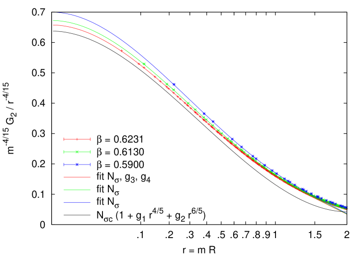
Figure 10: 2-point function divided by leading short-distance term versus $r^{2/5}$. Fit up to $g_{4}$ to $\beta=0.6231$ with range $[0.3,0.8]$ (red) and series up to $g_{4}$ with only $N_{\sigma}$ fitted to $\beta=0.613$ (green) and $\beta=0.59$ (blue) with ranges $[0.4,0.8]$ and $[0.6,1.0]$, resp. Theoretically known part of series up to $g_{2}$ with prefactor from continuum extrapolation of fig. 11 (black).

The scaling violations in $N_{\sigma}$ are expected to be of the form

$$N_{\sigma}(t)=N_{\sigma}^{c}(1+a_{N,\Delta}t^{\Delta}+\dots)$$ (89)

with the correction-to-scaling exponent $\Delta=2/3$ that already appeared in the discussion of the mass and the form factor in sect. 4.2. Remarkably, our crude estimates of $N_{\sigma}$ follow this prediction almost without deviation. Figure 11 shows a fit with $\Delta=2/3$ as well as a fit with two correction-to-scaling terms with exponents $2/3$ and $1$, which deviates only slightly. From the former, we obtain a continuum extrapolation of

$$N_{\sigma}^{c}=0.6376(6)$$ (90)

with the error taken as the difference of the two fits. Because of the unknown systematic errors in the individual $N_{\sigma}$, this error is probably strongly underestimated.

The short-distance expansion with this prefactor, and only including the analytically known terms up to $g_{2}$ is shown in fig. 10. The discrepancy between the data and this curve has two origins: scaling violations in the lattice data and omission of higher-order terms in the short-distance expansion. In the continuum limit, and with higher-order terms included, the two are expected to meet. The figure matches this expectation nicely.

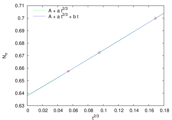
Figure 11: Scale dependence of $N_{\sigma}$.

The constant $N_{\sigma}$ plays the role of the normalization of the magnetization operator $\sigma_{\ell}$ on the lattice, and for this reason it is not calculable in the framework of field theory. It is a non-universal quantity which depends, among other things, upon the geometry of the lattice. In the case of the Ising model on a square lattice the analogous quantity can be evaluated exactly thanks to the fact that the $\sigma\bar{\sigma}$ correlator can be evaluated analytically on the lattice at the critical point. By comparing this result with the continuum-limit expression the normalization constant is then easily obtained (see for instance [40]). Unfortunately a similar exact lattice result does not exist for the three states Potts model on a triangular lattice.

6.2 Relation of short- and long-distance expansions

Given the normalization of the short-distance expansion $N_{\sigma}$, the amplitude of the 1-particle form factor $F^{\sigma}_{\bar{A}}$ can in principle be calculated in field theory using the cluster condition (24). The explicit form of $F^{\mu}_{\bar{A}A}(\theta)$ gives

$$\mathcal{N}\equiv\frac{F^{\sigma}_{\bar{A}}F^{\bar{\sigma}}_{A}}{\langle\mu\rangle^{2}}=0.968240\dots$$ (91)

The required amplitude of $\langle\mu\rangle$ in field theory, however, has not been computed so far. We can give an estimate of the latter using the measured values of $N_{\sigma}$ and $F_{\ell}$. Since $\sigma_{\ell}\simeq\sqrt{N_{\sigma}}\sigma$, the lattice and field theory form factors are related as $F_{\ell}=\sqrt{N_{\sigma}}F^{\sigma}_{\bar{A}}$.

In order to eliminate corrections to scaling, we extrapolate to the continuum limit. The scale dependence on the lattice was given in sect. 4.2 in terms of $t$,

$$F_{\ell} \sim F_{c}t^{1/9}$$ (92)

$$m \sim m_{c}t^{5/6}$$ (93)

while in field theory it is usually given in terms of the coefficient $\tau$ of the energy operator,

$$F^{\sigma}_{\bar{A}} \sim A_{F}\tau^{1/9}$$ (94)

$$m \sim A_{m}\tau^{5/6}\;.$$ (95)

The ratio $F^{\sigma}_{\bar{A}}/m^{2/15}$ is scale-independent. The corresponding amplitude ratio can thus be identified on the lattice and in field theory,

$$\frac{F_{c}/\sqrt{N_{\sigma}^{c}}}{m_{c}^{2/15}}=\frac{A_{F}}{A_{m}^{2/15}}\;.$$ (96)

The measured amplitudes (50) and (52) together with (90) yield the ratio

$$\frac{F_{c}/\sqrt{N_{\sigma}^{c}}}{m_{c}^{2/15}}=1.348(4)\;.$$ (97)

Using the known value $A_{m}=\kappa^{-5/6}=4.50431\dots$ from (66), we get

$$A_{F}=1.647(5)\;.$$ (98)

The amplitude of the disorder parameter is defined via

$$\langle\mu\rangle\sim A_{\mu}\tau^{1/9}\;.$$ (99)

The cluster condition (91) then gives $A_{\mu}=A_{F}/\sqrt{\mathcal{N}}$ and thus

$$A_{\mu}=1.674(5)\;.$$ (100)

All errors are probably underestimated, mainly because of the uncertainties in $N_{\sigma}^{c}$ as discussed in the previous section.

6.3 3-point correlator: Equilateral triangles

Let us write explicitly the perturbative expansion of the 3-point correlator in the case of the equilateral triangle. It will be useful in the perspective of a comparison between Monte-Carlo data and the form factor expansion worked out previously.

In such a particular case some simplifications occur, i.e. $|x_{i,j}|=R$ where $R$ is the side of the triangle. Then, with the choice (obviously the final results will be independent of such a choice)

$$x_{1}=0,\ \ \ x_{2}=R\,e^{i\pi/6},\ \ \ x_{3}=R\,e^{-i\pi/6}$$ (101)

we have

$${\tilde{y}}=i\,e^{-i\pi/6},\ \ \ 1-{\tilde{y}}=e^{-i\pi/3}$$ (102)

and finally

$${\mathcal{C}}_{\sigma\sigma\sigma}^{\epsilon}(0,R\,e^{i\pi/6},R\,e^{-i\pi/6};0)=C^{\bar{\sigma}}_{\sigma\sigma}C^{\epsilon}_{\sigma{\bar{\sigma}}}\,\left\{|f_{1}(i\,e^{-i\pi/6})|^{2}+K^{-1}|f_{2}(i\,e^{-i\pi/6})|^{2}\right\}R^{2/5}=C^{\epsilon}_{\sigma\sigma\sigma}\,R^{2/5}$$ (103)

where

$$C^{\epsilon}_{\sigma\sigma\sigma}=0.788825\dots.$$ (104)

Taking into account all the other pieces we have

$$G^{(3)}(R)=\frac{1}{R^{2/5}}\left\{C^{\bar{\sigma}}_{\sigma\sigma}+C^{\epsilon}_{\sigma\sigma\sigma}\,A_{\epsilon}\,\tau^{2/3}\,R^{4/5}+\dots\right\}.$$ (105)

Such an expression is very similar to the perturbative expansion of $\langle\sigma{\bar{\sigma}}\rangle$, in particular one can write it down using the dimensionless variable $u=\tau R^{6/5}$. As a consequence it is possible to guess the functional form of the higher order terms relying on dimensional analysis only. Hence we can write, in terms of $r=mR$,

$$G^{(3)}(R)=\frac{1}{R^{2/5}}\left(c_{1}+c_{2}\,r^{4/5}+c_{3}\,r^{6/5}+c_{4}\,r^{2}+c_{5}\,r^{12/5}+\dots\right)$$ (106)

where

$$c_{1}=C^{\bar{\sigma}}_{\sigma\sigma}=1.09236\dots\;,\ \ \ \ c_{2}=C^{\epsilon}_{\sigma\sigma\sigma}\,A_{\epsilon}\,\kappa^{2/3}=-2.29795\dots$$ (107)

and $c_{3},\dots$ are unknown (but in principle calculable) constants. It is also useful to define the scale invariant form of the correlator

$$\widetilde{G}^{(3)}(r)=m^{-2/5}\,\langle\sigma(x_{1})\sigma(x_{2})\sigma(x_{3})\rangle=\frac{1}{r^{2/5}}\left(c_{1}+c_{2}\,r^{4/5}+c_{3}\,r^{6/5}+c_{4}\,r^{2}+c_{5}\,r^{12/5}+\dots\right)$$ (108)

and its corresponding expression on the lattice

$$\widetilde{G}^{(3)}_{\ell}(r)=\frac{N_{\sigma}^{3/2}}{r^{2/5}}\left(c_{1}+c_{2}\,r^{4/5}+c_{3}\,r^{6/5}+c_{4}\,r^{2}+c_{5}\,r^{12/5}+\dots\right)$$ (109)

where $N_{\sigma}$ is (the square of) the normalization of the lattice magnetization operator. $N_{\sigma}$ has been extracted from the $\sigma\bar{\sigma}$ correlator in sect. 6.1. Since the scaling violations in the 3-point function are expected to be different from those in the 2-point function, we do not use the values of $N_{\sigma}$ fitted to the individual lattices, but rather the continuum extrapolation $N_{\sigma}^{c}$. The series up to the known $c_{2}$ with this prefactor is shown in fig. 12. Note that the abscissa is the distance between two spins (in physical units and to the power $2/5$), not the Y-length $mr_{\textrm{Y}}=\sqrt{3}r$ which appears in the long-distance expansion. The figure shows that, while higher-order terms are clearly important in the range where we have data, the leading term in the series is compatible with the latter.

A reasonable description of the data on the finest lattice can be obtained with the series up to $c_{5}$ with $N_{\sigma}$ and $c_{3},\dots,c_{5}$ as fit parameters. Like in the case of the 2-point function, we use a fit range where both lattice artifacts are small compared to uncorrelated statistical errors ($r\geq 0.3$) and the fit still works well ($r\leq 0.8$). The fit is shown in the fig. 12. Contrary to the case of the 2-point function, the fit does not stay near the data beyond the fit range, and, not surprisingly, the parameters depend quite strongly on the latter, see table 3. Since the fit already includes three terms, we do not attempt to estimate the effect of higher-order terms by including even more terms. The following uncertainties therefore contain neither the effects of these nor those of scaling violations:

$$N_{\sigma} =0.6376(36)$$ (110)

$$c_{3} =1.24(10)$$ (111)

$$c_{4} =0.44(45)$$ (112)

$$c_{5} =-0.33(37)\;.$$ (113)

Still, it is quite remarkable that the fit yields a value of $N_{\sigma}$ almost identical to the one extracted from the 2-point function (the near coincidence of the curves at $r=0$ in the figure is not enforced!)

$x_{\text{min}}$	$x_{\text{max}}$	$N_{\sigma}$	$c_{3}$	$c_{4}$	$c_{5}$
0.3	0.8	0.6376	1.240	$\phantom{-}0.441$	$-0.331$
0.15	0.5	0.6340	1.343	$-0.007$	$\phantom{-}0.042$
0.4	1.0	0.6365	1.255	$\phantom{-}0.393$	$-0.298$

Table 3: Results of fits to 3-point function at $\beta=0.6231$.

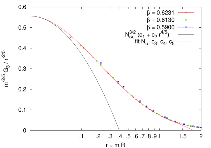
Figure 12: 3-point function divided by leading short-distance term, theoretically known part of series up to $c_{2}$ with prefactor from continuum extrapolation of $N_{\sigma}$ from 2-point function, and fit up to $c_{5}$ to the data at $\beta=0.6231$ in the range $[0.3,0.8]$.

Also contrary to the case of the 2-point function, the scaling violations on the coarser lattices cannot be described by just changing the prefactor $N_{\sigma}$. We do not attempt fits with more parameters as there is not a window where both lattice artifacts are small and higher-order terms can be neglected.

7 Implications for the three-quark potential

In these last years much interest has been attracted by the study of the three-quark potential in Lattice Gauge Theories (LGT). Besides the obvious phenomenological interest of the problem, the three-quark potential is also a perfect tool for testing our understanding of the flux tube model of confinement and of its theoretical description in terms of effective string models. These models have been elaborated in the past years looking at the quark-antiquark potential and their extension to baryonic states is highly non trivial. Thanks to the improvement in lattice simulations (a summary of numerical results can be found in [44]-[48]), the qualitative behaviour of the three-quark potential is now rather well understood (for a recent review see [42]).

• For large interquark distances the three-quark potential is well described by the so called Y law which assumes a flux tube configuration composed by three strings which originate from the three quarks and join in the Steiner point which has the property of minimizing the overall length of the three strings. This picture is also in agreement with what one would naively find using standard strong coupling expansion (notice however that due to the roughening transtion this is only a qualitative indication, and cannot be advocated as a“proof” of the Y law). An interesting consequence of this scenario is that one can use an effective string approach to model the behaviour of these flux tubes and hence a “Lüscher like” correction to the potential should be expected. This correction was evaluated in [46] and succesfully compared with simulations of the 3d ${\mathbb{Z}}_{3}$ gauge model in [42].

• At shorter distances a smooth crossover toward the so called $\Delta$ law is observed. According to the $\Delta$ law the three-quark potential is well approximated by the sum of the three two-quark interactions. More precisely the $\Delta$ law assumes that the three-quark correlator (let us call it $G_{3}(x_{1},x_{2},x_{3})$ where $x_{j}$ denotes the position of the $j^{th}$ quark) is related to the quark-antiquark correlator $G_{2}(x_{i},x_{j})$ as follows:

  $$G_{3}(x_{1},x_{2},x_{3})\sim\sqrt{G_{2}(x_{1},x_{2})~{}G_{2}(x_{2},x_{3})~{}G_{2}(x_{1},x_{3})}$$ (114)

  thus leading to a potential which increases linearly with the sum of the three interquark distances. The scale where the transition between these two behaviours seems to occur, according to the most recent simulation is around 0.8 fm.

To improve our understanding of the baryonic states it would be important now to have some quantitative insight in the above described picture as well as to have some theoretical argument to explain why instead of having a single shape stable for all the interquark distances a $\Delta\to Y$ crossover occurs. Moreover, since the crossover region happens to occur exactly in the range of distances which is interesting from a phenomenological point of view, it would be important to have some kind of theoretical description of this crossover with which to compare the numerical data.

In this respect the present study of the three-point function in the 2d ${\mathbb{Z}}_{3}$ Potts model is a perfect laboratory to address this problem. Besides the obvious similarity of the two settings it is also possible to find a direct relation, since by dimensional reduction the behaviour at high temperature of the three-quark correlator for a $SU(3)$ or a ${\mathbb{Z}}_{3}$ gauge model in (2+1) dimensions is mapped into the behvaiour of the 2d ${\mathbb{Z}}_{3}$ Potts three-point function (in analogy to what happens for the quark-antiquark potential which is mappend onto the $\langle\sigma\bar{\sigma}\rangle$ correlator).

This mapping becomes exact in the vicinity of the deconfinement transition thanks to the fact that both the deconfinement transition in the SU(3) LGT in (2+1) dimensions and the magnetization transition of the three-state Potts model in two dimensions are of second order. Then, according to the Svetitsky–Yaffe conjecture [49], the two critical points must belong to the same universality class and we can use the three-state Potts model as an effective theory for the SU(3) LGT. In this effective description the Polyakov loops of the LGT are mapped onto the spins of the Potts model, the confining phase of the LGT into the high temperature phase of the spin model while the combination $\sigma/T\equiv\sigma N_{t}$ (where $T$ is the finite temperature of the LGT model which is equivalent to the inverse of $N_{t}$: the lattice size in the timelike, compactified, direction) is mapped into the mass scale of the spin model (i.e. the inverse of the correlation length) and sets the scale of the deviations from the critical behaviour. It is exactly this scale which separates the $\Delta$ law behaviour from the Y one.

At the critical point (i.e. when the correlation length goes to infinity) the $\Delta$ law is exact. In fact looking at eq.(60) and (74) for the conformal two- and three-point correlators we see that the relation (114) is fulfilled exactly. On the other side, when the distances among the spins in the correlator are much larger than the correlation length, simple strong coupling arguments suggest that the dominating configuration in the partition function must be the one which minimizes the distances among the spins and the Y law appears. In field theory this behaviour for large separations among the spins is a direct consequence of the particle fusion process (8). Our analysis allows to follow in a rigorous way the crossover between the two limiting behaviours.

An interesting and non trivial application of our results is that they can give some insight on the high-temperature regime of the string corrections (the opposite of the one studied in [42]). This regime is reached when the interquark distances are much larger than the size of the lattice in the time direction and thus coincides (following the Svetitsky Yaffe mapping discussed above) with the large distance limit of the three-point correlator in the Potts model. A remarkable and not trivial feature of our result in this limit is that (when the Steiner point lies inside the triangle formed by the three spins) the dominating exponential behaviour is dressed by a pre-exponential factor $(r_{Y})^{-1/2}$ which is encoded in the $K_{0}$ modified Bessel function which appears in eq.(39). This is exactly the same behaviour of the two-point function in this limit and, as for the quark-antiquark case [50, 51], it indicates that in this limit the effective string corrections give a contribution proportional to $\log(r_{Y})$ (analogous of the $\log(r)$ term, with $r$ the interquark distance in the quark-antiquark case [50, 51, 52]). This is a rather non trivial result, which severely constraints the possible effective string pictures for the three quark potential and was indeed observed, in the free effective string limit in the case of the ${\mathbb{Z}}_{3}$ lattice gauge theory in three dimensions [53].

Acknowledgements: The work of P.G. is supported by the European Commission RTN Network EUCLID (contract HPRN-CT-2002-00325); M.C. and G.D. are also partially supported by this contract. O.J. is supported by funds provided by the U.S. Department of Energy (D.O.E.) under cooperative research agreement DE-FC02-94ER40818.

Appendix A

In order to show explicitly how to obtain equation (31), let us start from (30) and perform the change of variables $\beta\to\beta+i\alpha-i\pi/2$, $\theta\to\theta-i\gamma+i\pi/2$, so that we obtain

$$(F_{\bar{A}}^{\sigma})^{2}\int_{-\infty-i\alpha+i\pi/2}^{\infty-i\alpha+i\pi/2}\frac{\textrm{d}\beta}{2\pi}\int_{-\infty+i\gamma-i\pi/2}^{\infty+i\gamma-i\pi/2}\frac{\textrm{d}\theta}{2\pi}F_{AA}^{\sigma}(\beta-\theta+i(\alpha+\gamma))\exp\left[-m\left(R_{12}\cosh\beta+R_{23}\cosh\theta\right)\right].$$

Another change of variables, $\theta_{\pm}=\beta\pm\theta$, gives

$$\frac{(F_{\bar{A}}^{\sigma})^{2}}{2}\int_{-\infty-i\alpha_{-}}^{\infty-i\alpha_{-}}\frac{\textrm{d}\theta_{+}}{2\pi} \int_{-\infty-i\alpha_{+}+i\pi}^{\infty-i\alpha_{+}+i\pi}\frac{\textrm{d}\theta_{-}}{2\pi}\times$$

$$\times F_{AA}^{\sigma}(\theta_{-}+i\alpha_{+})\exp\left[-m\left(R_{12}\cosh\frac{\theta_{+}+\theta_{-}}{2}+R_{23}\cosh\frac{\theta_{+}-\theta_{-}}{2}\right)\right]$$

where $\alpha_{\pm}=\alpha\pm\gamma$. Now, we can integrate the function

$$f(\theta_{-})=F_{AA}^{\sigma}(\theta_{-}+i\alpha_{+})\exp\left[-m\left(R_{12}\cosh\frac{\theta_{+}+\theta_{-}}{2}+R_{23}\cosh\frac{\theta_{+}-\theta_{-}}{2}\right)\right]$$ (115)

on the complex $\theta_{-}$-plane along the contour ${\mathcal{C}}_{S}$ depicted in figure 13

$$\oint_{{\mathcal{C}}_{S}}f(\theta_{-})\,\textrm{d}\theta_{-}=U_{S}+D_{S}+R_{S}+L_{S}=-2\pi i\,H\left(\frac{2\pi}{3}-\alpha_{+}\right)\,\textrm{Res}_{\theta_{-}=\frac{2\pi i}{3}-i\alpha_{+}}f(\theta_{-})$$ (116)

where $H(z)$ is the usual step-function and

$$R_{S}=\int_{-S-i\alpha_{+}+i\pi}^{S-i\alpha_{+}+i\pi}\textrm{d}\theta_{-}\;f(\theta_{-}), L_{S}=\int_{-S}^{S}\textrm{d}\theta_{-}\;f(\theta_{-})$$

$$U_{S}=\int_{-S}^{-S-i\alpha_{+}+i\pi}\textrm{d}\theta_{-}\;f(\theta_{-}), D_{S}=\int_{S-i\alpha_{+}+i\pi}^{S}\textrm{d}\theta_{-}\;f(\theta_{-})\,.$$

The contribution of the pole is computed using the residue on the bound state

$$-i\;\textrm{Res}_{\theta_{-}=\frac{2\pi i}{3}-i\alpha_{+}}F_{AA}^{\sigma}(\theta_{-}+i\alpha_{+})=\Gamma^{\bar{A}}_{AA}F_{\bar{A}}^{\sigma}.$$

Then, taking the limit $S\to\infty$, both $U_{S}$ and $D_{S}$ vanish, and we are left with the following expression

$$(F_{\bar{A}}^{\sigma})^{2}\int_{-\infty}^{\infty}\frac{\textrm{d}\beta}{2\pi}\int_{-\infty}^{\infty}\frac{\textrm{d}\theta}{2\pi}\bigg{[}F_{AA}^{\sigma}(\beta-\theta+i(\alpha+\gamma))\exp\left[-m\left(R_{12}\cosh\beta+R_{23}\cosh\theta\right)\right]\bigg{]}+$$

$$+H\left(\frac{2\pi}{3}-\alpha_{+}\right)\;\frac{(F_{\bar{A}}^{\sigma})^{3}}{2}\;\Gamma^{\bar{A}}_{AA}\int_{-\infty}^{\infty}\frac{\textrm{d}\theta_{+}}{2\pi}\times$$

$$\hskip 5.69046pt\times\exp\left[-m\left(R_{12}\cosh\left(\frac{\theta_{+}}{2}+\frac{i\pi}{3}-i\alpha\right)+R_{23}\cosh\left(\frac{\theta_{+}}{2}-\frac{i\pi}{3}+i\gamma\right)\right)\right]\,.$$

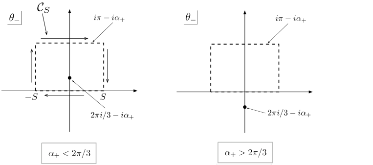
Figure 13: Contour of integration in the $\theta_{-}$ complex plane.

The desired result can be obtained in the following way. First, the expansion of the argument of the exponential function gives

$${\mathcal{R}}=R_{12}\cosh\left(\frac{\theta_{+}}{2}+\frac{i\pi}{3}-i\alpha\right)+R_{23}\cosh\left(\frac{\theta_{+}}{2}-\frac{i\pi}{3}+i\gamma\right)=$$

$$=\left[R_{12}\left(\cos\frac{\pi}{3}\cos\alpha+\sin\frac{\pi}{3}\sin\alpha\right)+R_{23}\left(\cos\frac{\pi}{3}\cos\gamma+\sin\frac{\pi}{3}\sin\gamma\right)\right]\cosh\frac{\theta_{+}}{2}+$$

$$+i\left[R_{12}\left(\sin\frac{\pi}{3}\cos\alpha-\cos\frac{\pi}{3}\sin\alpha\right)-R_{23}\left(\sin\frac{\pi}{3}\cos\gamma-\cos\frac{\pi}{3}\sin\gamma\right)\right]\sinh\frac{\theta_{+}}{2},$$

then taking into account the following geometric identities (figure 1)

$$r_{1}=R_{12}\frac{\sin\alpha}{\sin\frac{\pi}{3}},\ \ \ \ r_{3}=R_{23}\frac{\sin\gamma}{\sin\frac{\pi}{3}},$$

$$r_{2}=R_{12}\cos\alpha-r_{1}\cos\frac{\pi}{3}=R_{23}\cos\gamma-r_{3}\cos\frac{\pi}{3}$$

we finally have

$${\mathcal{R}}\ =\ (r_{1}+r_{2}+r_{3})\cosh\frac{\theta_{+}}{2}=r_{Y}\cosh\frac{\theta_{+}}{2}$$

and the term proportional to $\sinh\frac{\theta_{+}}{2}$ vanishes. Hence, by means of these simplifications we are able to obtain formula (31). Furthermore, with the same procedure it is possible to compute both eq.(3.4) and eq.(3.4).

Appendix B

A non-trivial check about the correlation functions written in section 3.1 (and as a consequence, about the form factors) is given by the computation of universal ratios. In particular, we are interested in those ratios which involve the amplitudes of the high-temperature ($\Gamma_{+}$) and “longitudinal” ($\Gamma_{-}$) and “transverse” ($\Gamma_{\textrm{\tiny T}}$) low-temperature magnetic susceptibilities. These ratios have been calculated in the continuum by form factors techniques in the kink basis of the low-temperature phase of the model with the result [9, 54]

$$\frac{\Gamma_{+}}{\Gamma_{-}}\simeq 13.85,\ \ \ \ \ \frac{\Gamma_{\textrm{\tiny T}}}{\Gamma_{-}}\simeq 0.327.$$ (118)

These values have been confirmed by lattice computations in [25] and [18]. The most accurate lattice estimates come from the latter paper and read $13.83(9)$ and $0.325(2)$, respectively.

Once duality is used to relate correlators in the two phases, the QFT resuls cannot depend on the regime used to compute the form factors. Hence, the results (118) must be reproduced in terms of the high-temperature form factors of the order and disorder operators we have used in this paper. Let us recall the definitions of the susceptibilities in terms of the correlators:

$$\chi_{+} = \int\textrm{d}^{2}x\;\langle\sigma_{\alpha}(x)\sigma_{\alpha}(0)\rangle_{T>T_{c}}$$

$$\chi_{-} = \int\textrm{d}^{2}x\;\langle 0_{\beta}|\sigma_{\beta}(x)\sigma_{\beta}(0)|0_{\beta}\rangle_{T<T_{c}}$$

$$\chi_{\textrm{\tiny T}} = \int\textrm{d}^{2}x\;\langle 0_{\beta}|\sigma_{\alpha}(x)\sigma_{\alpha}(0)|0_{\beta}\rangle_{T<T_{c}}\,,\ \ \ \ \ \alpha\neq\beta\,.$$ (119)

Here

$$\sigma_{\alpha}(x)=\delta_{s(x),\alpha}-\frac{1}{3},\ \ \ \ \ \ s(x)=0,1,2$$ (120)

and $|0_{\beta}\rangle$, $\beta=0,1,2$ are the vacua of the model in the low-temperature phase. The spin variables $\sigma$ and $\bar{\sigma}=\sigma^{*}$ we used in this paper read

$$\sigma(x)=e^{s(x)\frac{2\pi i}{3}},\ \ \ \ \ \ s(x)=0,1,2$$ (121)

so that

$$\sigma_{\alpha}(x)=\frac{1}{3}\left[\sigma(x)e^{-\alpha\frac{2\pi i}{3}}+\bar{\sigma}(x)e^{\alpha\frac{2\pi i}{3}}\right].$$ (122)

The correlators entering (119) can then be expressed in terms of those computed in this paper as

$$\langle\sigma_{\alpha}(x)\sigma_{\alpha}(0)\rangle_{T>T_{c}}=\frac{2}{9}\;\langle\sigma(x)\bar{\sigma}(0)\rangle_{T>T_{c}}$$ (123)

$$\langle 0_{\beta}|\sigma_{\alpha}(x)\sigma_{\alpha}(0)|0_{\beta}\rangle_{T<T_{c}}=\frac{2}{9}\;\langle\mu(x)\bar{\mu}(0)+\cos\frac{2\pi(\alpha-\beta)}{3}\;\mu(x)\mu(0)\rangle_{T>T_{c}}\,.$$ (124)

In the last equation duality has been used to trade $\sigma$ correlators at low-temperature for $\mu$ correlators at high-temperature. We can now use the form factors (23) to compute the susceptibilities up to two-particles

$$\chi_{+} \simeq {\mathcal{N}}\;\frac{\langle\mu\rangle^{2}}{m^{2}}\;0.44674$$

$$\chi_{-} \simeq \frac{\langle\mu\rangle^{2}}{m^{2}}\;0.0312375$$

$$\chi_{\textrm{\tiny T}} \simeq \frac{\langle\mu\rangle^{2}}{m^{2}}\;0.0102246$$ (125)

with ${\mathcal{N}}$ given in (91). Taking the ratios reproduces the results (118), as expected.

References

- [1] R. B. Potts, Proc. Camb. Phil. Soc. 48 (1952) 106.
- [2] F. Y. Wu, Rev. Mod. Phys. 54 (1982) 235; errata, ibid. 55 (1983) 315.
- [3] H. Feldmann, A. J. Guttmann, I. Jensen, R. Shrock and S.-H. Tsai, J. Phys. A 31, 2287 (1998), cond-mat/9801305.
- [4] S.-C. Chang, J. L. Jacobsen, J. Salas and R. Shrock, J. Stat. Phys. 114 (2004) 763, cond-mat/0211623.
- [5] D. Kim and R. J. Joseph, J. Phys. C 7 (1974) L167; T. W. Burkhardt and B. W. Southern, J. Phys. A 11 (1978) L247.
- [6] A. A. Belavin, A. M. Polyakov and A. B. Zamolodchikov, Nucl. Phys. B 241 (1984) 333.
- [7] V. A. Fateev and A. B. Zamolodchikov, Nucl. Phys. B 280 (1987) 644.
- [8] A.B. Zamolodchikov, Adv. Stud. Pure Math. 19 (1989) 641; Int. J. Mod. Phys. A 3 (1988) 743.
- [9] G. Delfino and J. L. Cardy, Nucl. Phys. B 519 (1998) 551 [arXiv:hep-th/9712111].
- [10] A. B. Zamolodchikov, Int. J. Mod. Phys. A 3 (1988) 743.
- [11] R. Köberle and J. A. Swieca, Phys. Lett. B 86 (1979) 209.
- [12] M. Karowski and P. Weisz, Nucl. Phys. B 139 (1978) 455.
- [13] F. A. Smirnov, Adv. Ser. Math. Phys. 14 (1992) 1.
- [14] V. P. Yurov and A. B. Zamolodchikov, Int. J. Mod. Phys. A 6 (1991) 3419.
- [15] A.N. Kirillov and F.A. Smirnov, ITF Kiev preprint ITF-88-73R (1988), in russian.
- [16] H. Babujian, A. Foerster and M. Karowski, hep-th/0510062.
- [17] G. Delfino, P. Simonetti and J. L. Cardy, Phys. Lett. B 387 (1996) 327 [arXiv:hep-th/9607046].
- [18] I. G. Enting and A. J. Guttmann, Physica A 321 (2003) 90.
- [19] L. Chim and A. B. Zamolodchikov, Int. J. Mod. Phys. A 7 (1992) 5317.
- [20] G. Delfino, G. Mussardo and P. Simonetti, Nucl. Phys. B 473 (1996) 469.
- [21] B. Nienhuis, J. Phys. A 15 (1982) 199.
- [22] J. Adler and V. Privman, J. Phys. A 15 (1982) L417;
- [23] G. von Gehlen, V. Rittenberg and T. Vescan, J. Phys. A 20 (1987) 2577.
- [24] S. L. A. de Queiroz, J. Phys. A 33 (2000) 721.
- [25] L. Shchur, P. Butera and B. Berche, Nucl. Phys. B 620 (2002) 579 [arXiv:cond-mat/0108005].
- [26] A. B. Zamolodchikov, Nucl. Phys. B 348 (1991) 619.
- [27] R. Guida and N. Magnoli, Nucl. Phys. B 471 (1996) 361 [arXiv:hep-th/9511209].
- [28] R. Guida and N. Magnoli, Nucl. Phys. B 483 (1997) 563 [arXiv:hep-th/9606072].
- [29] R. Guida and N. Magnoli, Int. J. Mod. Phys. A 13 (1998) 1145 [arXiv:hep-th/9612154].
- [30] S. L. Lukyanov and A. B. Zamolodchikov, Nucl. Phys. B 493 (1997) 571 [arXiv:hep-th/9611238].
- [31] V. Fateev, S. L. Lukyanov, A. B. Zamolodchikov and A. B. Zamolodchikov, Nucl. Phys. B 516 (1998) 652 [arXiv:hep-th/9709034].
- [32] V. Fateev, D. Fradkin, S. L. Lukyanov, A. B. Zamolodchikov and A. B. Zamolodchikov, Nucl. Phys. B 540 (1999) 587 [arXiv:hep-th/9807236].
- [33] V. S. Dotsenko and V. A. Fateev, Phys. Lett. B 154 (1985) 291.
- [34] T. R. Klassen and E. Melzer, Nucl. Phys. B 400 (1993) 547 [arXiv:hep-th/9110047].
- [35] J. McCabe and T. Wydro, Int. J. Mod. Phys. A 13 (1998) 1013.
- [36] V. A. Fateev, Phys. Lett. B 324 (1994) 45.
- [37] A. B. Zamolodchikov, Nucl. Phys. B 342 (1990) 695.
- [38] M. Caselle, P. Grinza and N. Magnoli, J. Phys. A 34 (2001) 8733 [arXiv:hep-th/0103263].
- [39] M. Caselle and M. Hasenbusch, Nucl. Phys. B 579 (2000) 667 [arXiv:hep-th/9911216].
- [40] M. Caselle, P. Grinza and N. Magnoli, Nucl. Phys. B 579 (2000) 635 [arXiv:hep-th/9909065].
- [41] F. Gliozzi and P. Provero, Phys. Rev. D 56 (1997) 1131 [arXiv:hep-lat/9701014].
- [42] P. de Forcrand and O. Jahn, Nucl. Phys. A 755 (2005) 475 [arXiv:hep-ph/0502039].
- [43] M. Lüscher, K. Symanzik and P. Weisz, Nucl. Phys. B173 (1980) 365.
- [44] C. Alexandrou, P. de Forcrand and A. Tsapalis, Phys. Rev. D 65 (2002) 054503 [arXiv:hep-lat/0107006].
- [45] C. Alexandrou, P. de Forcrand and O. Jahn, Nucl. Phys. Proc. Suppl. 119 (2003) 667 [arXiv:hep-lat/0209062].
- [46] O. Jahn and P. de Forcrand, Nucl. Phys. Proc. Suppl. 129 (2004) 700 [arXiv:hep-lat/0309115].
- [47] T. T. Takahashi et al., Phys. Rev. Lett. 86 (2001) 18 [arXiv:hep-lat/0006005].
- [48] T. T. Takahashi et al., Phys. Rev. D 65 (2002) 114509 [arXiv:hep-lat/0204011].
- [49] B. Svetitsky and L. G. Yaffe, Nucl. Phys. B 210 (1982) 423.
- [50] M. Lüscher and P. Weisz, JHEP 0407 (2004) 014 [arXiv:hep-th/0406205].
- [51] M. Billo and M. Caselle, JHEP 0507 (2005) 038 [arXiv:hep-th/0505201].
- [52] M. Caselle, M. Hasenbusch and M. Panero, JHEP 0301 (2003) 057 [arXiv:hep-lat/0211012].
- [53] P. de Forcrand and O. Jahn, unpublished.
- [54] G. Delfino, G. Barkema and J. Cardy, Nucl. Phys. B 565 (2000) 521.