Brane Decay of a (4+n)-Dimensional Rotating
Black Hole. II: spin-1 particles

M. Casals¹, P. Kanti² and E. Winstanley³

¹ School of Mathematical Sciences, University College Dublin,
Belfield, Dublin 4, Ireland

² Department of Mathematical Sciences, University of Durham,
Science Site, South Road, Durham DH1 3LE, United Kingdom

³ Department of Applied Mathematics, The University of Sheffield,
Hicks Building, Hounsfield Road, Sheffield S3 7RH, United Kingdom

Abstract

The present works complements and expands a previous one, focused on the emission of scalar fields by a $(4+n)$-dimensional rotating black hole on the brane, by studying the emission of gauge fields on the brane from a similar black hole. A comprehensive analysis of the particle, energy and angular momentum emission rates is undertaken, for arbitrary angular momentum of the black hole and dimensionality of spacetime. Our analysis reveals the existence of a number of distinct features associated with the emission of spin-1 fields from a rotating black hole on the brane, such as the behaviour and magnitude of the different emission rates, the angular distribution of particles and energy, the relative enhancement compared to the scalar fields, and the magnitude of the superradiance effect. Apart from their theoretical interest, these features can comprise clear signatures of the emission of Hawking radiation from a brane-world black hole during its spin-down phase upon successful detection of this effect during an experiment.

1 Introduction

One of the most exciting consequences of the scenario of Large Extra Dimensions [1] is that it opened the way for probing physics beyond the scale of quantum gravity by postulating the existence of a low fundamental gravitational scale $M_{*}$. If this scale is sufficiently low, trans-planckian particle collisions could easily be achieved in various environments. The products of such collisions cannot be ordinary particles any more but rather heavy or extended objects ($p$-branes, string balls, string states, etc) arising in the context of the more fundamental theory valid above $M_{*}$. As this ultimate fundamental theory should also include gravity, strong gravitational phenomena could also be observed at the quantum level, and the creation of tiny black holes as the result of trans-planckian collisions [2] is highly likely.

According to the theory with Large Extra Dimensions, all Standard Model fields are restricted to live on a (3+1)-dimensional brane, while gravity is allowed to propagate in the $(4+n)$-dimensional bulk (for some early works, see [3]). The theory predicts the existence of $n$ additional spacelike compact dimensions, all having – in the simplest case – the same size $L$. The collision of highly energetic particles on the brane may then produce a tiny black hole that is attached to our brane but, being a gravitational object, extends off our brane as well. In order to be able to treat the black hole as a classical object, it will be assumed that the black hole mass $M_{BH}$ is considerably larger than the fundamental scale of gravity $M_{*}$. Under the additional assumption that the horizon radius $r_{h}$ of the produced black hole is much smaller than the size of the extra compact dimensions $L$, this object can be considered to live in a $(4+n)$-dimensional non-compact, empty space; its properties differ from a 4-dimensional black hole with the same mass and strongly depend on the number $n$ of additional dimensions present [4].

Small higher-dimensional black holes may be created during trans-planckian collisions either at ground-based colliders [5] or in high energy cosmic-ray interactions in the atmosphere of the earth [6] (for an extensive discussion of the phenomenological implications and a more complete list of references, see the reviews [7, 8, 9]). After a short ‘balding’ phase, during which the black hole will shed all additional quantum numbers apart from its mass, angular momentum and charge, the more familiar Kerr-like phase commences, during which the black hole will lose mainly its angular momentum. After that, a Schwarzschild phase follows with the, now spherically-symmetric, black hole gradually losing its actual mass. The energy loss of the black hole takes place through the emission of Hawking radiation [10] (and through superradiance during its Kerr-like phase) that is, at the same time, the most prominent signature of black hole creation. This consists of the emission of elementary particles both in the bulk and on the brane, and it will be characterized by a very distinct thermal spectrum.

Due to the simplicity of the corresponding gravitational background that describes it, the Schwarzschild phase of the life of a small higher-dimensional black hole underwent an intensive and thorough study during recent years. The emission of Hawking radiation from such a black hole has been studied both analytically [11, 12, 13] and numerically [14]. These works have provided us with both analytical formulae and exact numerical results for the emission rates, and demonstrated how the latter strongly depend on the existence of additional spacelike dimensions in nature. As was shown in detail in [14], the number of particles and amount of energy emitted by the black hole per unit time was strongly enhanced by the presence of extra dimensions in the theory. Remarkably, it was found that the type of particles emitted also depends on how many dimensions exist in the bulk: scalar particles are predominantly emitted by a black hole living in a spacetime with a small number of (or no) extra dimensions, while gauge bosons are the preferred particles emitted by a black hole living in a spacetime with $n>5$. The spectrum of Hawking radiation may be a source of valuable information on other fundamental parameters of the theory, such as the value of the cosmological constant [15] and the string coupling associated with the presence of higher-derivative gravitational (Gauss-Bonnet) terms [16]. Other studies have focused on the effect of the mass of the emitted particles on the spectrum [17, 18] as well as the charge of the black hole [19].

Although initially almost totally ignored, the progress in studying the emission of Hawking radiation during the Kerr-like phase in the life of a small higher-dimensional black hole has been very rapid during the last year. Two early works [20, 21] focused on the special case of a 5-dimensional rotating black hole: the first one provided analytical formulae for the emission rates, and the second derived analytical results for the energy emission rate in the limit of low energy and low angular momentum of the black hole. The derivation of exact results valid for arbitrary values of the energy of the emitted particle and for arbitrary values of the angular momentum of the black hole required the numerical integration of both radial and angular parts of the equation of motion of the specific particle. The same task demands also the determination of the angular eigenvalue, that links radial and angular equations together, and which does not exist in closed form for arbitrary energy and angular momentum. The first exact numerical results for the emission of Hawking radiation from a $(4+n)$-dimensional rotating black hole, in the form of scalar fields, as well as for the energy amplification due to the superradiance effect, were presented in [22]. There it was shown that the energy emission is greatly enhanced by both the dimensionality of spacetime and the angular momentum of the black hole. In [23], results on the power (energy) spectrum, as well as its angular distribution in the 5-dimensional case were presented, but once more the analysis relied on the assumption of low energy and low angular momentum. Results on the superradiance effect in the case of a higher-dimensional black hole were also presented in [24] and [25], while the emission in the bulk was addressed in [26, 27].

Recently, a comprehensive study of the emission of Hawking radiation from a higher-dimensional black hole in its spin-down phase appeared in the literature [28]. This work focused on the emission of scalar fields on the brane, and presented exact results for the fluxes of particles, energy and angular momentum, for arbitrary values of the dimensionality of spacetime, angular momentum of the black hole, and energy of the emitted particle. Also, the angular distribution of the emitted radiation – a distinctive signature of emission from a rotating black hole – was investigated: it was demonstrated that the uniform distribution of particles in the case of a spherically-symmetric black hole is now replaced by a clearly oriented one that is transverse to the rotation axis of the black hole.

As the techniques used in the aforementioned work were strongly spin-dependent, the analysis for the emission of higher-spin fields was left for subsequent works. Here, we undertake the effort to fulfil this task for the case of gauge fields. As these fields are by definition restricted to live on the brane, only the brane emission channel will be studied. To this end, we will use semiclassical techniques that were originally developed for the case of 4-dimensional black holes and are here generalized to cover the case of higher-dimensional black hole line-elements projected onto a brane. As these techniques were developed particularly for the case of spin-1 particles, we are forced to leave the study of fermions for another work.

The outline of our paper is as follows: in Section 2, we present the theoretical framework for our analysis that includes the form of the gravitational background, and the derivation of the radial and angular part of the spin-1 equation of motion on the brane. In Section 3, we review, and generalize where necessary, the principles leading to the expressions for the transmission (or absorption) coefficient and of the various Hawking radiation emission fluxes. The techniques used to numerically integrate both the angular and radial parts of the spin-1 equation of motion – to derive the angular eigenvalue, the spin-weighted spheroidal harmonics, and the radial function – are described in detail in Section 4. The readers who are not interested in numerical techniques can move directly to Section 5, where our results are presented. Subsection 5.1 presents our results for the transmission coefficient and its behaviour in terms of the number of extra dimensions and angular momentum of the black hole. Subsections 5.2, 5.3 and 5.4 are devoted to the computation of the particle, energy and angular momentum fluxes, respectively: their dependence on both the dimensionality of spacetime and angular momentum of the black hole is investigated and, in the case of the first two types of fluxes, their angular distribution is also studied. Subsection 5.5 presents the total emissivities from a higher-dimensional rotating black hole on the brane in terms of the angular momentum, number of additional dimensions and azimuthal angle. The final subsection 5.6 addresses the issue of superradiance, and the energy amplification is computed in terms of the angular momentum and dimensionality of spacetime. We finish with a summary of our results and conclusions, in Section 6.

2 Gauge Field in a Brane-Induced Rotating Black Hole Background

As is well known, the generalization of the 4-dimensional, Kerr black hole background to a rotating, uncharged black hole living in a $(4+n)$-dimensional spacetime is given by the Myers-Perry solution [29]. Under the assumption that all ordinary matter – including ourselves – is restricted to live on a brane embedded in this background, we are interested in the type of line-element that describes the geometry on our brane. This follows by projecting the $(4+n)$-dimensional Myers-Perry background onto the brane, and is found to have the form [7]

$$\begin{split}ds^{2}=\left(1-\frac{\mu}{\Sigma\,r^{n-1}}\right)dt^{2}&+\frac{2a\mu\sin^{2}\theta}{\Sigma\,r^{n-1}}\,dt\,d\varphi-\frac{\Sigma}{\Delta}dr^{2}\\[8.53581pt] &-\Sigma\,d\theta^{2}-\left(r^{2}+a^{2}+\frac{a^{2}\mu\sin^{2}\theta}{\Sigma\,r^{n-1}}\right)\sin^{2}\theta\,d\varphi^{2}\,,\end{split}$$ (1)

where

$$\Delta=r^{2}+a^{2}-\frac{\mu}{r^{n-1}}\,,\qquad\Sigma=r^{2}+a^{2}\,\cos^{2}\theta\,.$$ (2)

The mass and angular momentum (transverse to the $r\varphi$-plane) of the black hole are then given by

$$M_{BH}=\frac{(n+2)A_{n+2}}{16\pi G}\,\mu\,,\qquad J=\frac{2}{n+2}\,M_{BH}\,a\,,$$ (3)

with $G$ being the $(4+n)$-dimensional Newton’s constant, and $A_{n+2}$ the area of an $(n+2)$-dimensional unit sphere, given by

$$A_{n+2}=\frac{2\pi^{(n+3)/2}}{\Gamma[(n+3)/2]}\,.$$ (4)

Above, we have assumed that the ($4+n$)-dimensional black hole was created by the collision of two highly energetic particles moving on our 3-brane. Assuming that the thickness of our brane is much smaller than the size $L$ of the extra dimensions, the two particles will have a non-zero impact parameter only along our brane; the produced black hole will therefore acquire only one non-zero angular parameter about an axis (the one transverse to the $r\varphi$-plane) in our brane.

The black hole horizon is given by solving the equation $\Delta(r)=0$, which, for $n\geq 1$, leads to a unique solution given by

$$r_{h}^{n+1}=\frac{\mu}{1+a_{*}^{2}}\,,$$ (5)

where we have defined $a_{*}=a/r_{h}$. We should note here that while for $n=0$ and $n=1$, there is a maximum possible value of $a$ that guarantees the existence of a real solution to the equation $\Delta=0$, for $n>1$ there is no fundamental upper bound on $a$ and a horizon $r_{h}$ always exists. An upper bound can nevertheless be imposed on the angular momentum parameter of the black hole by demanding the creation itself of the black hole from the collision of the two particles. The maximum value of the impact parameter between the two particles that can lead to the creation of a black hole was found to be [9]

$$b_{\text{max}}=2\,\biggl{[}1+\biggl{(}\frac{n+2}{2}\biggr{)}^{2}\biggr{]}^{-\frac{1}{(n+1)}}\mu^{\frac{1}{(n+1)}}\,,$$ (6)

an analytic expression that is in very good agreement with the numerical results produced in [2]c. Then, by writing $J=bM_{BH}/2$ [21], for the angular momentum of the black hole, and using Eq. (5) and the second of Eq. (3), we obtain

$$a^{\text{max}}_{*}=\frac{n+2}{2}\,.$$ (7)

We now proceed to derive the equation of motion of a gauge field in the induced-on-the-brane gravitational background (1). The quantization of an electromagnetic field on a rotating black hole background is considerably more involved than for a non-rotating black hole. While there is an extensive literature on the quantization of a scalar field on a Kerr black hole spacetime, rather less work has been done on spin-1 fields. For example, the first comprehensive study of the stress-energy tensor on the entire geometry has only been recently undertaken [30]. However, the formalism itself has been sufficiently well developed for our purposes for Kerr black holes [30, 31, 32, 33, 34, 35, 36, 37, 38] and, here, we shall extend this to the more general background metric (1). In this section, we will only outline the key features of the theory, referring the interested reader to [30] (and references therein) for further details.

We use the Newman-Penrose formalism [39] to derive the equations for the electromagnetic field components, written in terms of the Newman-Penrose scalars:

$$\phi_{-1}\equiv F_{{\mbox{\boldmath{$l$}}}{\mbox{\boldmath{$m$}}}}\,;\qquad\phi_{0}\equiv\left(F_{{\mbox{\boldmath{$l$}}}{\mbox{\boldmath{$n$}}}}+F_{{\mbox{\boldmath{$m$}}}^{*}{\mbox{\boldmath{$m$}}}}\right)/2\,;\qquad\phi_{+1}\equiv F_{{\mbox{\boldmath{$m$}}}^{*}{\mbox{\boldmath{$n$}}}}\,,$$ (8)

where $\{{\mbox{\boldmath{$l$}}},{\mbox{\boldmath{$n$}}},{\mbox{\boldmath{$m$}}},{\mbox{\boldmath{$m$}}}^{*}\}$ are the null basis vectors. Here, we follow the notation of [30, 40, 41], and use the subscript $h$ on $\phi$, taking the values (0, $\pm$1), to describe the helicity of the spin-1 field – note that both helicities ($h=\pm 1$) will contribute to the Hawking radiation. We should emphasize that, in our terminology, helicity is in effect a label for the field modes, and we do not strictly link this to any particular physical field configuration. This latter point is explored in more detail in [30, 42].

The tetrad we use is the Kinnersley tetrad [33], which readily generalizes to the metric (1) with $\Delta$ given by Eq. (2) rather than the usual Kerr metric form. The analysis of Teukolsky [31, 32] showed that the partial differential equations for $\phi_{-1}$ and $\rho^{-2}\phi_{+1}$ [where $\rho=-1/(r-ia\cos\theta)$ is one of the spin coefficients] are in this case separable. It is straightforward to show that this result also extends to our more general situation. The Maxwell scalars (8) can be decomposed into a Fourier mode sum

$$\phi_{h}=\int_{-\infty}^{+\infty}\,d{\omega}\sum_{\ell=|h|}^{+\infty}\,\sum_{m=-\ell}^{+\ell}\,\sum_{P=\pm 1}{}_{h}a_{\ell m\omega P}\,{}_{h}\phi_{\ell m\omega}\,,$$ (9)

where ${}_{h}a_{\ell m\omega P}$ are the coefficients of the Fourier series. The parameter $\ell$ labels the eigenvalues of the angular Teukolsky equation (see Eq. (13) below). The parameter $P$ is summed in (9) over the values $+1$ and $-1$, corresponding to the two linearly independent polarization states of the electromagnetic potential. An electromagnetic potential mode of polarization $P$ is an eigenstate of the parity operator

$$\mathcal{P}:(\theta,\phi)\to(\pi-\theta,\phi+\pi)\,.$$ (10)

with eigenvalue $P$. The decomposition of the potential into eigenstates of the parity operator $\mathcal{P}$ is the natural choice due to the invariance of the metric (1) under this operation. The Fourier modes in (9) are then separated according to

$${}_{\pm 1}\phi_{\ell m\omega}={}_{\pm 1}N_{\ell m\omega}\,\rho^{(1\pm 1)}\,{}_{\mp 1}R_{\ell m\omega}(r)\,{}_{\mp 1}Z_{\ell m\omega}(\theta,\varphi)\,e^{-i\omega t}\,,$$ (11)

where ${}_{\pm 1}N_{\ell m\omega}$ is a suitable normalization constant, ${}_{\mp 1}R_{\ell m\omega}(r)$ is a radial function and ${}_{\mp 1}Z_{\ell m\omega}(\theta,\varphi)$ is the angular function. The equation for the Maxwell scalar $\phi_{0}$ is not separable; instead, this scalar can be written in terms of the radial and angular functions for $h=\pm 1$. The answer is given explicitly in [30, 33, 35] for Kerr black holes ($n=0$), but here we do not need it further. The Fourier modes of the electromagnetic potential can be reconstructed from the Maxwell scalars ${}_{\pm 1}\phi_{\ell m\omega}$ – explicit formulae for this are given in [30, 34], again for Kerr black holes.

The angular function ${}_{h}Z_{\ell m\omega}(\theta,\varphi)$ is defined as

$${}_{h}Z_{\ell m\omega}(\theta,\varphi)\equiv\frac{(-1)^{m+1}}{\sqrt{2\pi}}\,{}_{h}S_{\ell m\omega}(\theta)\,e^{+im\varphi}\,,$$ (12)

where ${}_{h}S_{\ell m\omega}(\theta)$ is the spin-weighted spheroidal harmonic [43, 44, 45, 46, 47, 48, 49]. Introducing the new variable $x=\cos\theta$, the latter satisfies the equation

$$\left[\frac{d}{dx}\left((1-x^{2})\frac{d}{dx}\right)+a^{2}\omega^{2}x^{2}-2ha\omega x-\frac{(m+hx)^{2}}{1-x^{2}}+{}_{h}\mathcal{A}_{\ell m\omega}+h\right]{}_{h}S_{\ell m\omega}(x)=0\,.$$ (13)

In the above, ${}_{h}\mathcal{A}_{\ell m\omega}$ is the separation constant, usually written as

$${}_{h}\mathcal{A}_{\ell m\omega}={}_{h}\lambda_{\ell m\omega}-a^{2}\omega^{2}+2ma\omega,$$ (14)

with ${}_{h}\lambda_{\ell m\omega}$ regarded as the eigenvalue of the equation (13). The spin-weighted spheroidal harmonics satisfy the following symmetry relations:

$${}_{h}S_{\ell m\omega}(\theta) = (-1)^{\ell+m}\,{}_{-h}S_{\ell m\omega}(\pi-\theta)$$

$${}_{h}S_{\ell m\omega}(\theta) = (-1)^{\ell+h}\,{}_{h}S_{\ell-m-\omega}(\pi-\theta)$$

$${}_{h}S_{\ell m\omega}(\theta) = (-1)^{h+m}\,{}_{-h}S_{\ell-m-\omega}(\theta)\,,$$ (15)

and are normalized according to

$$\int_{0}^{\pi}d\theta\sin\theta\,{}_{h}S_{\ell m\omega}^{2}(\theta)=1.$$ (16)

The solution of the angular equation (13) is discussed in Section 4.

The radial function ${}_{h}R_{\ell m\omega}(r)$, on the other hand, is found to satisfy the following equation

$$\Delta^{-h}\,\frac{d}{dr}\left(\Delta^{h+1}\,\frac{d{}_{h}R_{\ell m\omega}}{dr}\right)+{}_{h}V\,{}_{h}R_{\ell m\omega}=0\,.$$ (17)

For $h=+1$, the potential ${}_{h}V={}_{+1}V$ is given by [7, 21]

$${}_{+1}V=\frac{K^{2}-iK\Delta^{\prime}}{\Delta}+4i\omega r+\left(\Delta^{\prime\prime}-2\right)-{}_{+1}\lambda_{\ell m\omega}\,,$$ (18)

where we have defined: $K=(r^{2}+a^{2})\,\omega-am$. Throughout this work, we use a prime $(^{\prime})$ to denote a derivative with respect to the radial coordinate $r$. For both Kerr ($n=0$) and 5-dimensional Kerr-like black holes of the form given in Eq. (1), the term $\Delta^{\prime\prime}-2$ vanishes identically. The $h=+1$ radial equation (17) with the potential (18) fits the pattern of the master equation found for various spins in [7, 21]. However, there is a rather surprising result for helicity $h=-1$, when the radial function ${}_{-1}R_{\ell m\omega}(r)$ still satisfies (17) but the potential ${}_{-1}V$ has a different form:

$${}_{-1}V=\frac{K^{2}+iK\Delta^{\prime}}{\Delta}-4i\omega r-{}_{-1}\lambda_{\ell m\omega}.$$ (19)

Note that the $\Delta^{\prime\prime}-2$ term is absent in this case. Thus, while the master equation in [7, 21] describes the helicity $h=+1$ radial functions, it does not describe the helicity $h=-1$ radial functions. We suspect that something similar may happen with spin-1/2 fields as well. The solution of the radial equation (17) is also described in detail in Section 4.

3 Hawking radiation in the form of gauge fields

For an evaporating black hole on the brane, the relevant quantum state is the (“past”) Unruh vacuum $|U^{-}\rangle$. There are some subtleties in the construction of this state for an electromagnetic field on a rotating black hole background which are described in detail in [30]. The field is expanded in terms of the usual “in” and “up” modes, for which the radial functions ${}_{h}R_{\ell m\omega}(r)$ have the asymptotic forms [30]:

$${}_{h}R^{\text{in}}_{\ell m\omega} \sim \begin{cases}{}_{h}R^{\text{in,tra}}_{\ell m\omega}\,\Delta^{-h}\,e^{-i\tilde{\omega}r_{*}}&(r\rightarrow r_{h})\\[5.69054pt] {}_{h}R^{\text{in,inc}}_{\ell m\omega}\,\frac{\textstyle e^{-i\omega r_{*}}}{\textstyle r}+{}_{h}R^{\text{in,ref}}_{\ell m\omega}\,\frac{\textstyle e^{+i\omega r_{*}}}{\textstyle r^{1+2h}}&(r\rightarrow+\infty)\end{cases}$$ (20)

$${}_{h}R^{\text{up}}_{\ell m\omega} \sim \begin{cases}{}_{h}R^{\text{up,inc}}_{\ell m\omega}\,e^{+i\tilde{\omega}r_{*}}+{}_{h}R^{\text{up,ref}}_{\ell m\omega}\,\Delta^{-h}\,e^{-i\tilde{\omega}r_{*}}&\qquad(r\rightarrow r_{h})\\[5.69054pt] {}_{h}R^{\text{up,tra}}_{\ell m\omega}\,\frac{\textstyle e^{+i\omega r_{*}}}{\textstyle r^{1+2h}}&\qquad(r\rightarrow+\infty)\,.\end{cases}$$ (21)

In the above, we have used the abbreviation

$${\tilde{\omega}}=\omega-m\Omega,$$ (22)

with $\Omega$ the horizon angular velocity

$$\Omega=\frac{a_{*}}{(1+a_{*}^{2})\,r_{h}}\,,$$ (23)

and the usual tortoise coordinate $r_{*}$ defined through the relation

$$\frac{dr_{*}}{dr}=\frac{r^{2}+a^{2}}{\Delta(r)}\,.$$ (24)

The coefficients ${}_{h}R^{\text{in,tra}}_{\ell m\omega}$, ${}_{h}R^{\text{in,inc}}_{\ell m\omega}$, ${}_{h}R^{\text{in,ref}}_{\ell m\omega}$, ${}_{h}R^{\text{up,inc}}_{\ell m\omega}$, ${}_{h}R^{\text{up,ref}}_{\ell m\omega}$, ${}_{h}R^{\text{up,tra}}_{\ell m\omega}$ appearing in Eqs. (20) and (21) are arbitrary integration constants. The correct expression for the unrenormalized expectation value of the stress-energy tensor in the state $|U^{-}\rangle$ is given in terms of a mode sum as follows [30]:

$$\langle U^{-}|T_{\mu\nu}|U^{-}\rangle = \frac{1}{2}\sum_{\ell mP}\left(\int_{0}^{\infty}d{\tilde{\omega}}\,\coth\left(\frac{\pi\tilde{\omega}}{\kappa_{+}}\right)\right.$$ (25)

$$\qquad\qquad\times\left\{T_{\mu\nu}\left[{}_{h}\phi_{\ell m\omega}^{\text{up}},{}_{h}\phi_{\ell m\omega}^{\text{up}*}\right]+(-1)^{\vartheta}\mathcal{P}\left(T_{\mu\nu}\left[{}_{h}\phi_{\ell m\omega}^{\text{up}},{}_{h}\phi_{\ell m\omega}^{\text{up}*}\right]\right)\right\}$$

$$\left.+\int_{0}^{\infty}d{\omega}\,\left\{T_{\mu\nu}\left[{}_{h}\phi_{\ell m\omega}^{\text{in}},{}_{h}\phi_{\ell m\omega}^{\text{in}*}\right]+(-1)^{\vartheta}\mathcal{P}\left(T_{\mu\nu}\left[{}_{h}\phi_{\ell m\omega}^{\text{in}},{}_{h}\phi_{\ell m\omega}^{\text{in}*}\right]\right)\right\}\right),$$

where the quantity $T_{\mu\nu}\left[{}_{h}\phi_{\ell m\omega},{}_{h}\phi_{\ell m\omega}^{*}\right]$ is the classical electromagnetic stress-energy tensor

$$T_{\mu\nu}\left[{}_{h}\phi_{\ell m\omega},{}_{h}\phi_{\ell m\omega}^{*}\right] = \left\{{}_{-1}\phi_{\ell m\omega}\,{}_{-1}\phi_{\ell m\omega}^{*}{\mbox{\boldmath{$n$}}}_{\mu}{\mbox{\boldmath{$n$}}}_{\nu}+2\,{}_{0}\phi_{\ell m\omega}\,{}_{0}\phi_{\ell m\omega}^{*}\left[{\mbox{\boldmath{$l$}}}_{(\mu}{\mbox{\boldmath{$n$}}}_{\nu)}+{\mbox{\boldmath{$m$}}}_{(\mu}{\mbox{\boldmath{$m$}}}_{\nu)}^{*}\right]\right.$$ (26)

$$+_{+1}\phi_{\ell m\omega}\,{}_{+1}\phi_{\ell m\omega}^{*}{\mbox{\boldmath{$l$}}}_{\mu}{\mbox{\boldmath{$l$}}}_{\nu}-4\,{}_{0}\phi_{\ell m\omega}\,{}_{-1}\phi_{\ell m\omega}^{*}{\mbox{\boldmath{$n$}}}_{(\mu}{\mbox{\boldmath{$m$}}}_{\nu)}$$

$$\left.-4\,{}_{+1}\phi_{\ell m\omega}\,{}_{0}\phi_{\ell m\omega}^{*}{\mbox{\boldmath{$l$}}}_{(\mu}{\mbox{\boldmath{$m$}}}_{\nu)}+2\,{}_{+1}\phi_{\ell m\omega}\,{}_{-1}\phi_{\ell m\omega}^{*}{\mbox{\boldmath{$m$}}}_{\mu}{\mbox{\boldmath{$m$}}}_{\nu}\right\}$$

$$+{\mbox{complex conjugate}},$$

given in terms of the tetrad basis vectors. In (25), the variable $\vartheta$ has been defined so that $(-1)^{\vartheta}$ is equal to $-1$ if one index of the component of the stress tensor is $\theta$ and the other one is not, and it is equal to $+1$ otherwise. The key feature of the unrenormalized $\langle U^{-}|T_{\mu\nu}|U^{-}\rangle$ (25) is the term involving the parity operator ${\mathcal{P}}$ (10). This ensures that the stress-energy tensor as a whole is invariant under the parity operator.

Our interest in this paper is in the outgoing fluxes of particles $N$, energy $E$ and angular momentum $J$, which means that we do not need to compute all the components of the renormalized stress-energy tensor. We require only the components $T_{tr}$ and $T_{r\varphi}$, and our analysis is further simplified by the fact that these components do not require renormalization. This latter fact is proved for a quantum scalar field in [50]. Their argument is, however, purely geometric, and can readily be extended to the case of an electromagnetic field, thereby showing that the counterterms in Ref. [51] vanish for these components of the stress-energy tensor. In addition, a similar argument can be used to show that the linearly divergent term [52] also vanishes for these components. We may then use the results [30, 50]

$$\frac{dE}{dt} = \int_{S_{\infty}}d\theta\,d\varphi\,r^{2}\sin\theta\,\langle U^{-}|T^{tr}|U^{-}\rangle,$$

$$\frac{dJ}{dt} = \int_{S_{\infty}}d\theta\,d\varphi\,r^{2}\sin\theta\,\langle U^{-}|T^{r}_{\varphi}|U^{-}\rangle,$$ (27)

where the integration is taken over the sphere at infinity. The contribution to $T_{tr}$ for an “up” mode takes the form:

$$\Delta\left(T_{tr}{}_{\ell m\omega}^{\text{up}}+\mathcal{P}T_{tr}{}_{\ell m\omega}^{\text{up}}\right)=$$

$$\qquad\qquad\frac{\mathbb{T}_{\ell m\omega}}{4\pi^{2}\Sigma}\Big{\{}-\omega\Sigma\left({}_{-1}S_{\ell m\omega}^{2}+{}_{+1}S_{\ell m\omega}^{2}\right)+\frac{a^{3}\cos\theta\sin^{2}\theta}{\Sigma}\left({}_{-1}S_{\ell m\omega}^{2}-{}_{+1}S_{\ell m\omega}^{2}\right)$$

$$\qquad\qquad+a\sin\theta\left({}_{-1}S_{\ell m\omega}\partial_{\theta}{}_{-1}S_{\ell m\omega}-{}_{+1}S_{\ell m\omega}\partial_{\theta}{}_{+1}S_{\ell m\omega}\right)\Big{\}}.$$ (28)

In the above equation, ${\mathbb{T}}_{\ell m\omega}$ is the transmission coefficient, defined as a ratio of energy fluxes:

$$\mathbb{T}_{\ell m\omega}=\frac{dE^{\text{(tra)}}_{\ell m\omega}/dt}{dE^{\text{(inc)}}_{\ell m\omega}/dt},$$ (29)

with $E^{\text{(inc)}}$ and $E^{\text{(tra)}}$ denoting, respectively, the incident energy on the black hole and the energy transmitted down the event horizon. The quantity ${\mathbb{T}}_{\ell m\omega}$ is the analogue of the “absorption probability” defined in [28]. The transmission coefficient ${\mathbb{T}}_{\ell m\omega}$ can be written in terms of $W[{}_{+1}R,{}_{-1}R^{*}]^{\text{in}}_{\ell m\omega}$, the Wronskian of the “in” mode radial functions, as follows [30]:

$$\mathbb{T}_{\ell m\omega}=\frac{-i}{2^{4}\omega^{3}}W[{}_{+1}R,{}_{-1}R^{*}]^{\text{in}}_{\ell m\omega},$$ (30)

where we have chosen the normalization ${}_{-1}R^{\text{in,inc}}_{\ell m\omega}={}_{-1}R^{\text{up,inc}}_{\ell m\omega}=1$. The contribution to $T_{tr}$ for an “in” mode is the same as for an “up” mode but with a change of sign. There are also similar expressions describing the contributions to $T_{r\varphi}$ for both the “in” and “up” modes.

For the fluxes in which we are interested, only the behaviour of the stress tensor at infinity is needed. As $r\rightarrow\infty$, the expression (3) simplifies to:

$$\left(T_{tr}{}_{\ell m\omega}^{\text{up}}+\mathcal{P}T_{tr}{}_{\ell m\omega}^{\text{up}}\right)\sim-\frac{\mathbb{T}_{\ell m\omega}}{4\pi^{2}r^{2}}\omega\left({}_{-1}S_{\ell m\omega}^{2}+{}_{+1}S_{\ell m\omega}^{2}\right)\,.$$ (31)

It is important to note that both the positive and negative helicity angular functions contribute to this expression. In [21], only one helicity was included for each mode, which resulted in the angular distributions in that paper being highly asymmetric about the equator. By using the correct expression given above, we will find later that the angular distributions are in fact symmetric about the equator, as would be expected from a physical point of view.

We now use (31) and the corresponding result for $T_{r\varphi}$ to find the following formulae for the differential emission rates of particles, energy and angular momentum, integrated over all angles $\theta$, as a function of the mode energy $\omega$:

$$\frac{d^{2}N}{dtd\omega} = \frac{1}{2\pi}\sum_{\ell=1}^{\infty}\sum_{m=-\ell}^{\ell}\sum_{P=\pm 1}\frac{1}{\exp\left(\tilde{\omega}/T_{\text{H}}\right)-1}{\mathbb{T}}_{\ell m\omega}\,,$$ (32)

$$\frac{d^{2}E}{dtd\omega} = \frac{1}{2\pi}\sum_{\ell=1}^{\infty}\sum_{m=-\ell}^{\ell}\sum_{P=\pm 1}\frac{\omega}{\exp\left(\tilde{\omega}/T_{\text{H}}\right)-1}{\mathbb{T}}_{\ell m\omega}\,,$$ (33)

$$\frac{d^{2}J}{dtd\omega} = \frac{1}{2\pi}\sum_{\ell=1}^{\infty}\sum_{m=-\ell}^{\ell}\sum_{P=\pm 1}\frac{m}{\exp\left(\tilde{\omega}/T_{\text{H}}\right)-1}{\mathbb{T}}_{\ell m\omega}\,,$$ (34)

as well as the angular distributions of particles and energy:

$$\frac{d^{3}N}{d(\cos\theta)dtd\omega} = \frac{1}{4\pi}\sum_{\ell=1}^{\infty}\sum_{m=-\ell}^{\ell}\sum_{P=\pm 1}\frac{1}{\exp\left(\tilde{\omega}/T_{\text{H}}\right)-1}{\mathbb{T}}_{\ell m\omega}\left({}_{-1}S_{\ell m\omega}^{2}+{}_{+1}S_{\ell m\omega}^{2}\right)\,,$$ (35)

$$\frac{d^{3}E}{d(\cos\theta)dtd\omega} = \frac{1}{4\pi}\sum_{\ell=1}^{\infty}\sum_{m=-\ell}^{\ell}\sum_{P=\pm 1}\frac{\omega}{\exp\left(\tilde{\omega}/T_{\text{H}}\right)-1}{\mathbb{T}}_{\ell m\omega}\left({}_{-1}S_{\ell m\omega}^{2}+{}_{+1}S_{\ell m\omega}^{2}\right)\,,$$ (36)

where $T_{\text{H}}$ is the Hawking temperature of the $(4+n)$-dimensional, rotating black hole, given by

$$T_{\text{H}}=\frac{(n+1)+(n-1)\,a_{*}^{2}}{4\pi\,(1+a_{*}^{2})\,r_{h}}\,.$$ (37)

An important part of the above expressions is the sum over the polarization $P$, which is in agreement with [53]. The transmission coefficient ${\mathbb{T}}_{\ell m\omega}$ is independent of $P$, so in effect we simply multiply by a factor of 2. As in [28], we do not study the angular behaviour of $T_{r\varphi}$ (corresponding to an angular distribution of the flux of angular momentum) as it will not be directly observable. However, for the interested reader, $T_{r\varphi}$ is studied for the 4-dimensional Kerr black hole in [30].

Let us finally note here that the emission of Hawking radiation will be assumed to take place through the emission of gauge particles with energy much smaller than the mass of the black hole. This will guarantee that there is no significant back reaction to the gravitational background due to the change in the black hole mass after the emission of a particle. Since the black hole radiation spectrum is centered around the temperature of the black hole, we must demand that $T_{\text{H}}\ll M_{BH}$. This eventually translates to $M_{BH}\gg M_{*}$, a condition that has already been imposed to guarantee the absence of any quantum corrections to our analysis.

4 Numerical Analysis

The greybody factor, or transmission coefficient ${\mathbb{T}}_{\ell m\omega}$, given by Eq. (30), can be calculated from the solutions of the radial Teukolsky equation (17) for propagation on the brane black hole background; however, we still need to solve the angular equation (13) since its eigenvalue appears in the radial equation. We will also require the spin-weighted spheroidal harmonics themselves for the angular distributions of the particle and energy fluxes (35, 36). In this section, we briefly outline the numerical methods used to solve both the angular and radial equations of a spin-1 field in the aforementioned black hole background.

In order to solve the angular equation, we use the shooting method as described in [43]. This method is based on the one applied in [28, 54] to solve the spin-0 spheroidal harmonic equation, and here we adapt it to the non-zero spin case. We start by using the Frobenius method, and re-write the angular function as follows:

$${}_{h}S_{\ell m\omega}(x)=(1-x)^{\alpha_{+}}(1+x)^{\alpha_{-}}{}_{h}y_{\ell m\omega}(x)\,,$$ (38)

where

$$\alpha_{+} =\frac{|m+h|}{2}\,, \qquad\qquad\alpha_{-} =\frac{|m-h|}{2}\,.$$ (39)

The function ${}_{h}y_{\ell m\omega}(x)$ then satisfies the differential equation

$$\Bigg{\{}(1-x^{2})\frac{d^{2}}{dx^{2}}-2\left[\alpha_{+}-\alpha_{-}+(\alpha_{+}+\alpha_{-}+1)x\right]\frac{d}{dx}+{}_{h}\lambda_{\ell m\omega}+h(h+1)-a^{2}\omega^{2}$$ (40)

$$\qquad\qquad\qquad\quad+2ma\omega-(\alpha_{+}+\alpha_{-})(\alpha_{+}+\alpha_{-}+1)+a^{2}\omega^{2}x^{2}-2ha\omega x\Bigg{\}}{}_{h}y_{\ell m\omega}(x)=0\,.$$

From Eq. (40), it is clear that ${}_{h}y^{\prime\prime}_{\ell m\omega}$ cannot be calculated at exactly the end-points $x=\pm 1$ since these are (regular) singular points. We will, therefore, integrate this equation from the point $x_{1}\equiv-1+\epsilon$ up to the point $x_{2}\equiv+1-\epsilon$, where $\epsilon\ll 1$.

The shooting method for solving Eq. (40) requires an ansatz, ${}_{h}\hat{\lambda}_{\ell m\omega}$, for the eigenvalue ${}_{h}\lambda_{\ell m\omega}$ of the angular equation. Imposing regularity of the solution at $x=-1$ determines the values of ${}_{h}y_{\ell m\omega}$ and ${}_{h}y^{\prime}_{\ell m\omega}$ at $x_{1}$, up to an arbitrary overall normalization. The equation is then integrated from $x_{1}$ to $x_{2}$, as an initial value problem. If the solution obtained at $x_{2}$ does not comply with the boundary condition of regularity at $x=+1$, the value of ${}_{h}\hat{\lambda}_{\ell m\omega}$ is improved. The differential equation is then integrated again with the new value of ${}_{h}\hat{\lambda}_{\ell m\omega}$ until regularity at $x=+1$ is met within the desired accuracy; the derived solution for the spin-weighted spheroidal harmonics is then normalized so that Eq. (16) is satisfied.

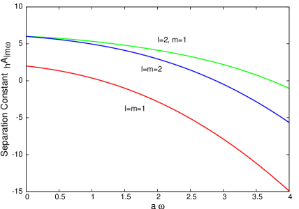
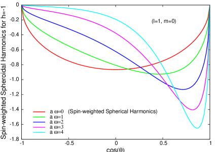
Figure 1: (a) The separation constant ${}_{h}\mathcal{A}_{\ell m\omega}(a\omega)$, for the modes $\ell=m=1,2$ and $\ell=2,m=1$, and helicity $h=-1$; (b) Spin-1 weighted spheroidal harmonics for a gauge field with $h=-1$, $\ell=1$, $m=0$, and for $a\omega=(0,1,2,3)$.

For an ansatz ${}_{h}\hat{\lambda}_{\ell m\omega}$ for the angular eigenvalue, the numerical solution ${}_{h}y^{\text{num}}_{\ell m\omega}$ of Eq. (40) is a combination of both a regular and an irregular solution, i.e.

$${}_{h}y^{\text{num}}_{\ell m\omega}=A({}_{h}\hat{\lambda}_{\ell m\omega})\,{}_{h}y_{\ell m\omega}+B({}_{h}\hat{\lambda}_{\ell m\omega})\,{}_{h}y^{\text{irreg}}_{\ell m\omega}\,,$$ (41)

where ${}_{h}y_{\ell m\omega}$ and ${}_{h}y^{\text{irreg}}_{\ell m\omega}$ are the regular and irregular solutions at $x=\pm 1$, respectively, and $A$ and $B$ unknown functions of ${}_{h}\hat{\lambda}_{\ell m\omega}$. The value of ${}_{h}\hat{\lambda}_{\ell m\omega}$ must be modified so that only the regular term $A\,{}_{h}y_{\ell m\omega}$ is retained. For general spin, this is achieved by requiring that ${}_{h}\hat{\lambda}_{\ell m\omega}$ is a zero of the function

$$g({}_{h}\hat{\lambda}_{\ell m\omega})\equiv{}_{h}y^{{}^{\prime}\text{num}}_{\ell m\omega}(x_{2})-{}_{h}y^{{}^{\prime}\text{approx}}_{\ell m\omega}(x_{2})\,,$$ (42)

where ${}_{h}y^{{}^{\prime}\text{approx}}_{\ell m\omega}(x_{2})$ is an approximation to the (unknown) regular value:

$${}_{h}y_{\ell m\omega}^{{}^{\prime}\text{approx}}(x_{2})\simeq\frac{{}_{h}y^{\text{num}}_{\ell m\omega}(x_{2})}{{}_{h}y_{\ell m\omega}(x_{2})}\,{}_{h}y^{\prime}_{\ell m\omega}(x_{2})\,.$$ (43)

The fraction ${}_{h}y^{\prime}_{\ell m\omega}(x_{2})/{}_{h}y_{\ell m\omega}(x_{2})$ can be found analytically by calculating a series expansion of ${}_{h}y_{\ell m\omega}$ around $x=+1$. This series and further details can be found in [42]. As an illustrative result, in Fig. 1, we depict the value of the separation constant ${}_{h}\mathcal{A}_{\ell m\omega}$ = ${}_{h}\lambda_{\ell m\omega}+\\ 2ma\omega-a^{2}\omega^{2}$, and of the spin-1 weighted spheroidal harmonics for various field modes.

Once the eigenvalues of the angular equation (13) are found, we can proceed to solve the radial equation (17). The radial Teukolsky equation in four dimensions contains a long-range potential in the spin-1 case, which cannot readily be integrated numerically. We use the following definition of long/short-rangeness [57]: a second-order differential equation

$$\frac{d^{2}Y(x)}{dx^{2}}+{\mathcal{A}}(x)\,\frac{dY(x)}{dx}+{\mathcal{B}}(x)\,Y(x)=0$$ (44)

is said to be short-range if, and only if, ${\mathcal{A}}(x)=O(x^{-d})$ and ${\mathcal{B}}(x)=b_{\pm}^{2}+O(x^{-d})$, where $d\geq 2$ and $b_{\pm}$ are constants, when $x\to\pm\infty$. If this condition is guaranteed, then the asymptotic form of the solution is

$$Y(x)\sim\begin{cases}e^{\pm ib_{+}x}&(x\to+\infty)\\ e^{\pm ib_{-}x}&(x\to-\infty)\,.\end{cases}$$ (45)

Detweiler showed [55, 56] that a particular transformation from the radial function ${}_{-1}R_{\ell m\omega}$ to a new radial function $X_{\ell m\omega}$ leads to a differential equation which is real and contains a short-range potential in terms of the tortoise co-ordinate $r_{*}$ (24). This new differential equation, being short-range (in the homogeneous case), is suitable for numerical integration. This method is followed and detailed in [30] for the four dimensional, Kerr-Newman case.

In this work, we have followed Detweiler’s method and generalized his differential equation valid for the Kerr black hole to any 4-dimensional line-element of the form (1), including the case of a higher-dimensional black hole background induced on the brane. It can be easily checked that the Teukolsky-Starobinskiĭ identities [33, 38] are valid for a general metric function $\Delta(r)$; in particular,

$${}_{+1}R_{\ell m\omega}=2\left(\frac{d}{dr}-\frac{iK}{\Delta}\right)\left(\frac{d}{dr}-\frac{iK}{\Delta}\right){}_{-1}R_{\ell m\omega}\,.$$ (46)

It can also be easily checked that the same is true for all the formulae in [55] until we reach the point where the potential is written out explicitly, i.e. Eq. (61) in [55]. For a general function $\Delta$, we define a new radial function $X_{\ell m\omega}$ according to

$$X_{\ell m\omega}\equiv(r^{2}+a^{2})^{1/2}\Delta^{-1/2}\chi_{\ell m\omega}\,,$$ (47)

where

$$\chi_{\ell m\omega}=\alpha\,{}_{-1}R_{\ell m\omega}+\beta\,\frac{d{}_{-1}R_{\ell m\omega}}{dr}\,.$$ (48)

The functions $\alpha$ and $\beta$ appearing in the definition of $\chi_{\ell m\omega}$ are quite complex. To define them, first write $\alpha$ and $\beta$ in terms of two new quantities $p$ and $q$ as follows:

$$\alpha=p+a_{D}q\,,\qquad\qquad\beta=b_{D}q\,,$$ (49)

where

$$a_{D} = -\frac{2}{\Delta}\left[2K^{2}+\Delta(iK^{\prime}-{}_{-1}\lambda_{\ell m\omega})\right]\,,$$

$$b_{D} = \frac{4iK}{\Delta}\,.$$ (50)

The $p$ and $q$ functions are then themselves defined as

$$p = {}_{1}B_{\ell m\omega}\left(\frac{2K^{2}}{\Delta}-{}_{-1}\lambda_{\ell m\omega}+{}_{1}B_{\ell m\omega}\right)^{-1/2}\,,$$

$$q = \frac{p\Delta}{2{}_{1}B_{\ell m\omega}}\,,$$ (51)

where, finally,

$${}_{1}B_{lm\omega}^{2}={}_{-1}\lambda_{lm\omega}^{2}+4ma\omega-4a^{2}\omega^{2}\,.$$ (52)

The function $X_{\ell m\omega}$ now satisfies the differential equation

$$\frac{d^{2}X_{\ell m\omega}}{dr_{*}^{2}}-{}_{-1}\mathcal{U}X_{\ell m\omega}=0\,,$$ (53)

with

$${}_{-1}\mathcal{U} =\frac{\Delta{}_{-1}\lambda_{\ell m\omega}-K^{2}}{(r^{2}+a^{2})^{2}}+\frac{\Delta^{2}(Kp^{\prime})^{\prime}}{(r^{2}+a^{2})^{2}Kp}-\left(\frac{\Delta}{r^{2}+a^{2}}\right)^{3/2}\left[\frac{\Delta^{1/2}}{(r^{2}+a^{2})^{1/2}}\right]^{\prime\prime}\,.$$ (54)

Note that the signs of $a_{D}$ and $b_{D}$ above differ from those in [55] so that the sign in the Teukolsky-Starobinskiĭ identity (46) agrees with that in [38].

The explicit form of the potential (54) given by Detweiler uses $\Delta=r^{2}-2Mr+a^{2}$, and therefore it only applies to the four dimensional, Kerr background. Here, we have calculated it for a general function $\Delta(r)$, and the result is:

$${}_{-1}\mathcal{U} =-\frac{\left[\omega(r^{2}+a^{2})-am\right]^{2}}{(r^{2}+a^{2})^{2}}+\frac{\Delta{}_{-1}\lambda_{\ell m\omega}}{(r^{2}+a^{2})^{2}}$$ (55)

$$-\frac{\Delta\left\{2(2r^{2}-a^{2})\Delta+(r^{2}+a^{2})\left[\Delta^{\prime\prime}(r^{2}+a^{2})-2r\Delta^{\prime}\right]\right\}}{2(r^{2}+a^{2})^{4}}$$

$$-\frac{\Delta\left\{2(5r^{2}+\nu^{2})\Delta-(r^{2}+\nu^{2})\left[5r\Delta^{\prime}+\frac{\Delta^{\prime\prime}}{2}(r^{2}+\nu^{2})\right]\right\}}{(r^{2}+a^{2})^{2}\left[(r^{2}+\nu^{2})^{2}+\eta\Delta\right]}$$

$$+\frac{6r(r^{2}+\nu^{2})^{2}\Delta\left[2r\Delta-(r^{2}+\nu^{2})\Delta^{\prime}\right]}{(r^{2}+a^{2})^{2}\left[(r^{2}+\nu^{2})^{2}+\eta\Delta\right]^{2}}-\frac{\eta\Delta\left(\Delta^{\prime}\right)^{2}\left[2(r^{2}+\nu^{2})^{2}-\eta\Delta\right]}{4(r^{2}+a^{2})^{2}\left[(r^{2}+\nu^{2})^{2}+\eta\Delta\right]^{2}}\,,$$

where

$$\nu^{2} \equiv a^{2}-am/\omega\,,$$ (56)

$$\eta \equiv\frac{{}_{1}B_{\ell m\omega}-{}_{-1}\lambda_{\ell m\omega}}{2\omega^{2}}\,.$$

When $\Delta(r)$ is given by Eq. (2), the potential ${}_{-1}\mathcal{U}$ is found to be real and short-range, for any number of extra dimensions $n\geq 0$. That is, the differential equation (53) is short-range, in terms of $r_{*}$, in both limits $r\to+\infty$ and $r\to r_{h}$ for any $n\geq 0$. Furthermore, it can be checked that this differential equation is short-range, in terms of the independent variable $r$, in the limit $r\to+\infty$, for $n\geq 1$. Note, however, that it is not short-range in terms of $r$ in the limit $r\to r_{h}$ for any $n\geq 0$.

The relation $r_{*}=r_{*}(r)$ can be easily found in closed form in the cases $n=0\to 3$ but not in the cases $n=4\to 7$. We, therefore, found it useful to define a new variable $r_{\Delta}$ such that $r_{\Delta}$ behaves like $r_{*}$, for $r\to r_{h}$, and like $r$, for $r\to+\infty$ (to ensure short-rangeness), and such that we can find the relation $r_{\Delta}=r_{\Delta}(r)$ in closed form $\forall n\geq 1$. The differential equation will be short-range (for $n\geq 1$) with respect to this new radial variable, both for $r\to r_{h}$ and $r\to+\infty$. A radial variable $r_{\Delta}$ that satisfies these properties can be defined via

$$\frac{dr_{\Delta}}{dr}\equiv\frac{r}{r-r_{h}}\,.$$ (57)

The relation $r_{\Delta}=r_{\Delta}(r)$ in closed form is then given by

$$r_{\Delta}=r+r_{h}\log\left(\frac{r-r_{h}}{r_{h}}\right)\,.$$ (58)

This relation can be inverted with the use of Lambert’s W function [58] to yield

$$r=r_{h}\left[W\left(\frac{1}{r_{h}}\,e^{(r_{\Delta}-r_{h})/r_{h}}\right)+1\right]\,.$$ (59)

Note that $r_{\Delta}\sim r_{*}$, as $r\to r_{h},+\infty$. If Eq. (53) is re-expressed in terms of $r_{\Delta}$, the resulting differential equation is

$$\frac{d^{2}X_{\ell m\omega}}{dr_{\Delta}^{2}}+\frac{(r-r_{h})\left[rF_{\Delta}^{\prime}(r^{2}+a^{2})+F_{\Delta}(a^{2}-r^{2})\right]}{r^{2}F_{\Delta}(r^{2}+a^{2})}\,\frac{dX_{\ell m\omega}}{dr_{\Delta}}-\left(\frac{r^{2}+a^{2}}{rF_{\Delta}}\right)^{2}{}_{-1}\mathcal{U}(r)X_{\ell m\omega}=0\,,$$ (60)

where

$$F_{\Delta}\equiv\frac{\Delta}{r-r_{h}}$$ (61)

is finite at the horizon. In this work, we numerically solved the differential equation (53) in the cases $n=0\to 3$, and the differential equation (60) in the cases $n=4\to 7$.

As in [28], we solved the radial equation (either (53) or (60) as applicable), to find the “in” modes, for which the function $X_{\ell m\omega}$ has the asymptotic forms

$$X^{\text{in}}_{\ell m\omega} \sim\begin{cases}B^{\text{in}}_{\ell m\omega}\,e^{-i\tilde{\omega}r_{*}}&(r\rightarrow r_{h})\\[5.69054pt] e^{-i\omega r_{*}}+A^{\text{in}}_{\ell m\omega}\,e^{+i\omega r_{*}}&(r\rightarrow+\infty)\,.\end{cases}$$ (62)

Our ultimate aim is to calculate the greybody factor $\mathbb{T}_{\ell m\omega}$. To find an expression for this in terms of the function $X_{\ell m\omega}$, we first note that the inverse of relation (48) is given in [55], and it is equally valid for a general function $\Delta(r)$:

$${}_{-1}R_{\ell m\omega}=\left[\alpha\left(\alpha+\beta^{\prime}\right)-\beta\left(\alpha^{\prime}+\frac{\beta}{\Delta}\,{}_{-1}V\right)\right]^{-1}\left[\left(\alpha+\beta^{\prime}\right)\chi_{\ell m\omega}-\beta\,\frac{d\chi_{\ell m\omega}}{dr}\right]\,.$$ (63)

Using this relation, we can obtain the coefficients of the radial Teukolsky function ${}_{-1}R^{\text{in}}_{\ell m\omega}$ at $r\to+\infty$, which correspond to the normalization chosen in Eq. (62):

$$\frac{{}_{-1}R^{\text{in,ref}}_{\ell m\omega}}{{}_{-1}R^{\text{in,inc}}_{\ell m\omega}A^{\text{in}}_{\ell m\omega}} =\frac{4\omega^{2}}{{}_{1}B_{\ell m\omega}}\,, \qquad\quad{}_{-1}R^{\text{in,inc}}_{\ell m\omega} =\frac{1}{2^{3/2}|\omega|}\,.$$ (64)

These expressions, together with Eq. (30), allow us to obtain the following simple expression for the greybody factor:

$$\mathbb{T}_{\ell m\omega}=\frac{\tilde{\omega}}{\omega}\,|B^{\text{in}}_{\ell m\omega}|^{2}\,.$$ (65)

By using the above result, we may then proceed to compute the fluxes of particles, energy and angular momentum, given in Eqs. (32–36), by a brane-induced black hole.

5 Numerical Results

We now turn to the presentation of the exact numerical results, first, for the transmission coefficient and, subsequently, for the flux, power and angular momentum spectra for the emission of gauge fields on the brane from a higher-dimensional, rotating black hole. As in the case of the emission of scalar fields [28], we wish to study the dependence of the various emission rates on the dimensionality of spacetime $n$ and the angular momentum parameter $a_{*}$. Also, the angular distribution of the emitted number of particles and energy will be derived – as we will see, the particular shape of the angular distribution comprises a clear signature not only of the emission during the spin-down phase in the life of the black hole but also of the type of emitted particles. Finally, the total emissivities of flux, power and angular momentum, as well as the superradiance effect, will be discussed, and more particularly their dependence on the two fundamental parameters $n$ and $a_{*}$.

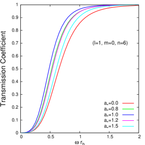
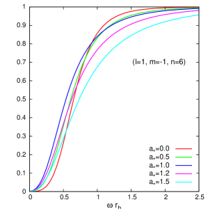
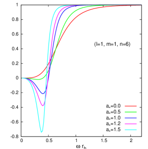
Figure 2: Transmission coefficients for spin-1 emission on the brane from a 10-dimensional black hole with variable $a_{*}$, for the modes (a) $\ell=1,m=0$, (b) $\ell=1,m=-1$ and (c) $\ell=1,m=1$.

5.1 Transmission Coefficient

We start the presentation of our results with the ones for the transmission coefficient $\mathbb{T}_{\ell m\omega}$, as these follow from the numerical solution of the radial equations (53) and (60) by using as input the exact eigenvalue ${}_{-1}\lambda_{\ell m\omega}$. As we will see, the transmission coefficient bears a strong dependence on both the angular momentum parameter $a_{*}$ of the black hole and the number of additional spacelike dimensions $n$. In addition, its behaviour depends on the particular mode studied as well as on the energy regime that is investigated.

Figure 2 depicts the dependence of $\mathbb{T}_{\ell m\omega}$ on the angular momentum parameter $a_{*}$ – for simplicity, the number of extra dimensions has been fixed to $n=6$. The three panels show the modes ($\ell=1,m=0$), ($\ell=1,m=-1$) and ($\ell=1,m=1$), and reveal the non-monotonic behaviour of $\mathbb{T}_{\ell m\omega}$ as $a_{*}$ varies. For the ($\ell=1,m=0$) mode, the transmission coefficient first increases and then decreases, as $a_{*}$ increases. This behaviour is justified by, and reflected in, the behaviour of the gravitational potential (55) seen by the propagating gauge field: as $a_{*}$ starts increasing, the barrier lowers, thus giving a boost to $\mathbb{T}_{\ell m\omega}$; as $a_{*}$ increases further, however, the one-peak potential changes to a double-peak form with the height of the peak located closer to the horizon increasing with $a_{*}$, which leads to a suppression of the transmission coefficient.

For the ($l=1,m=-1$) mode, the behaviour of $\mathbb{T}_{\ell m\omega}$ is found to be $\omega$-dependent, too. For low values of $\omega$, as $a_{*}$ starts increasing, the one-peak potential tends to become significantly more localized, leading to the observed enhancement of the transmission coefficient. For large values of $\omega$, the gravitational barrier changes to a well whose depth increases with $a_{*}$, thus suppressing the value of $\mathbb{T}_{\ell m\omega}$. The dependence on $\omega$ is even more striking for the third depicted mode ($\ell=1,m=1$). This mode is a ‘superradiant’ mode, one that is characterized by a negative value of the transmission coefficient over the energy regime $\tilde{\omega}=\omega-m\Omega<0$, according to Eq. (65), and thus by a value of the reflection coefficient larger than unity (see also section 5.6). For fixed dimensionality, Fig. 2(c) reveals that $\mathbb{T}_{\ell m\omega}$ is greatly suppressed with $a_{*}$ over the superradiance regime but enhanced everywhere else. The behaviour of the potential again supports the observed behaviour: in the low-energy regime, an increase in $a_{*}$ either raises the barrier or deepens the well that characterizes the gravitational potential, thus suppressing the transmission coefficient to even smaller values; in the high-energy regime, as $a_{*}$ increases, the potential is characterized by the simultaneous presence of a barrier and a well, whose height and depth, respectively, decrease as $a_{*}$ increases, thus justifying the observed enhancement.

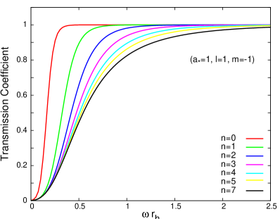
\psfrag{x}[0.8]{$\omega\,r_{\text{h}}$}\psfrag{y}[0.8]{$r_{\text{h}}^{2}\,d^{2}N/dt\,d\omega$}\includegraphics[height=162.18062pt,clip]{greyl1m1a1.eps}

Figure 3: Transmission coefficients for spin-1 emission on the brane from a black hole with $a_{*}=1$ and variable $n$, for the modes (a) $\ell=1,m=-1$, and (b) $\ell=1,m=1$.

The dependence of the transmission coefficient on the dimensionality of spacetime is depicted in Fig. 3, for a fixed value of the angular momentum parameter, i.e. $a_{*}=1$. The left panel depicts the behaviour of a non-superradiant mode – in this case the $\ell=1$, $m=-1$ mode – and reveals the suppression of $\mathbb{T}_{\ell m\omega}$, as $n$ increases. The above monotonic behaviour holds for all non-superradiant modes, with $m\leq 0$, and in all energy regimes. The right panel of Fig. 3 shows the behaviour of the corresponding superradiant mode ($l=1$, $m=1$), in which we observe that the supression of $\mathbb{T}_{\ell m\omega}$ with the number of extra spacelike dimensions holds also for this type of modes. The suppression is present also in the superradiant regime, where an increase in the value of $n$ leads to a further suppression (larger negative value) of the transmission coefficient. In terms of the gravitational potential, one may easily see that, for all modes, the height of the barrier – or, the depth of the well, depending on the values of $a_{*}$ and $\omega$ – increases as $n$ increases, thus justifying the behaviour depicted in Fig. 3.

The various emission spectra – particle, energy and angular momentum – as well as their dependence on the parameters $a_{*}$ and $n$, will be determined by the behaviour of both the transmission coefficient $\mathbb{T}_{\ell m\omega}$ and the thermal factor ($e^{\tilde{\omega}/T_{\text{H}}}-1)^{-1}$, appearing in Eqs. (32)-(34). Having discussed the behaviour of the transmission coefficient, let us now comment on the dependence of the thermal factor on $n$ and $a_{*}$. The behaviour of the latter on the number of additional dimensions is encoded in the expression of the temperature of the black hole, given in Eq. (37). A simple study reveals that, for $a_{*}$ and $r_{h}$ fixed, $\partial T_{\text{H}}/\partial n>0$, and the temperature of the black hole always increases with the value of $n$, thus giving a boost to the thermal factor and, therefore, to all emission spectra. As the thermal factor behaves in exactly the opposite way from the transmission coefficient in terms of $n$, it remains to be seen which of the two is the prevailing factor that determines the behaviour of the final emission spectra.

The dependence of the thermal factor on $a_{*}$ is more elaborate: in this case we find that, for $n$ and $r_{h}$ fixed,

$$\frac{\partial}{\partial a_{*}}\left(\frac{\omega-m\Omega}{T_{\text{H}}}\right)=4\pi r_{h}\,\frac{ma_{*}^{2}\,(n-1)+4a_{*}\omega-m\,(n+1)}{[\,(n+1)+(n-1)\,a_{*}^{2}\,]^{2}}\,,$$ (66)

according to which the behaviour of the thermal factor, as $a_{*}$ varies, depends on the particular mode, the energy and angular-momentum regime, and the dimensionality of spacetime. For modes with $m=0$, the behaviour of the $(\omega-m\Omega)/T_{\text{H}}$ is monotonic, and increases with $a_{*}$ for all values of $n$ and $\omega$, leading to the suppression of the thermal factor and thus of the various emission spectra. Combining this result with the behaviour of the transmission coefficient depicted in Fig. 2(a), we may conclude that the $m=0$ modes will significantly contribute to the various spectra only for black holes with an angular momentum in the low $a_{*}$-regime, where the suppression of the thermal factor is small and the transmission coefficient is enhanced. Turning to the modes with $m<0$, we find that, for $n\leq 1$, the r.h.s of Eq. (66) is always positive, and the various spectra are suppressed for all $a_{*}$ and $\omega$; for $n>1$, the thermal factor is found to be again suppressed in the low $a_{*}$-regime but significantly enhanced in the high $a_{*}$-regime and low $\omega$-regime. According to Fig. 2(b), the transmission coefficient will also be enhanced for these values of $a_{*}$ and $\omega$, therefore, modes with $m<0$ will be mainly emitted in the low-energy regime from black holes with a large angular momentum. Finally, for modes with $m>0$, we need to distinguish between the superradiant and non-superradiant energy regimes. In the latter one, we find that the thermal factor is actually suppressed with $a_{*}$, while, according to Fig. 2(c), the transmission coefficient is enhanced; it is, therefore, the ‘battle’ between these two quantities that will define the final spectrum for modes with $m>0$ in the non-superradiant regime. For modes with $m>0$ and energy in the superradiant regime $\omega-m\Omega<0$, the situation changes radically: the thermal factor is found to be suppressed with $a_{*}$, however, its value is now negative. Since this is the energy regime over which the transmission coefficient also acquires a negative value, the Hawking radiation flux remains positive and it is actually significantly enhanced with $a_{*}$ as both the thermal factor and $\mathbb{T}_{\ell m\omega}$ are driven towards larger negative values, as $a_{*}$ increases.

In the next three subsections, we present the various emission spectra for spin-1 fields by using the results derived above. Their final expressions (32)-(36) involve a sum over both $m\in[-\ell,\ell]$ and $\ell\in[1,\infty)$, thus rendering them mode-independent. Although this makes the contribution of individual modes impossible to discern, the derived spectra will be the combined effect of all radiated modes and contributing factors.

5.2 Flux emission spectra

The number of gauge bosons emitted by the black hole on the brane per unit time and unit frequency was computed first, by using Eq. (32). Our results are presented in Figs. 4 and 5, in terms of the dimensionless  energy parameter $\omega r_{h}$, and for fixed dimensionality and angular momentum parameter of the black hole, respectively.

\psfrag{x}[0.8]{$\omega\,r_{\text{h}}$}\psfrag{y}[0.8]{${r_{\text{h}}^{2}\,d^{2}N/dt\,d\omega}$}\includegraphics[height=159.3356pt,clip]{fluxs1n1.eps} \psfrag{x}[0.8]{$\omega\,r_{\text{h}}$}\psfrag{y}[0.8]{$r_{\text{h}}^{2}\,d^{2}N/dt\,d\omega$}\includegraphics[height=159.3356pt,clip]{fluxs1n6.eps}

Figure 4: Flux emission spectra for spin-1 particles on the brane from a rotating black hole, for (a) $n=1$, and (b) $n=6$, and various values of $a_{*}$.             

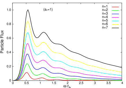
Figure 5: Flux emission spectra for spin-1 particles on the brane from a rotating black hole, with $a_{*}=1$, for various values of $n$.             

Figures 4(a,b) depict the particle emission rate for a 5-dimensional ($n=1$) and a 10-dimensional ($n=6$) black hole, respectively, and for various values of $a_{*}$. Both plots reveal the clear enhancement in the number of particles emitted per unit time and frequency by the black hole, as the angular momentum of the black hole increases. In both cases, this enhancement is observed over the whole energy band, but the exact form of the spectrum depends strongly on the dimensionality of spacetime: for low values of $n$, there is a clear preference for the emission of low-energy gauge bosons, although the emission of particles with higher energy becomes increasingly more likely, as the angular momentum increases; for high values of $n$, the emission of low-energy quanta is still favoured but the probability for the emission of high-energy ones has become substantially more important than the one in the low-dimensional case. The spectra in both cases are characterized by oscillations caused by the higher partial waves coming gradually into dominance as the energy increases.

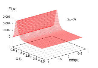
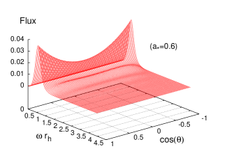
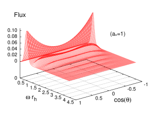
Figure 6: Angular distribution of the flux spectra for gauge boson emission on the brane from a rotating black hole, for $n=1$ and $a_{*}=(0,0.6,1)$.

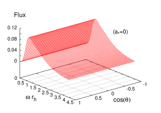
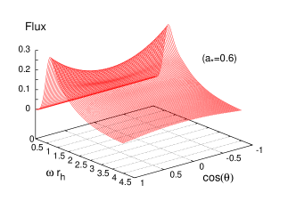
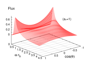
Figure 7: Angular distribution of the flux spectra for gauge boson emission on the brane from a rotating black hole, for $n=6$ and $a_{*}=(0,0.6,1)$.

As is well known from previous studies, an increase in the dimensionality of spacetime causes a significant enhancement in the number of particles emitted per unit time and frequency by the black hole; this effect was observed in the case of a higher-dimensional Schwarzschild [11, 13, 14], Schwarzschild-de-Sitter [15], and Schwarzschild-Gauss-Bonnet [16] black hole, as well as in the case of scalar emission from a higher-dimensional Kerr-like black hole [22, 28]. The same enhancement is anticipated in the present case of the emission of gauge bosons, and this behaviour can be readily seen by comparing the vertical axes of Figs. 4(a) and (b). A more complete picture can be drawn from Fig. 5, where the flux spectrum is given for fixed angular momentum ($a_{*}=1$) and variable $n$. As we see, the particle emission curves become significantly taller and broader, as $n$ increases, which signals the enhancement of the total emissivity of the black hole by virtually orders of magnitude.

We now turn to the angular distribution of the flux spectra: we study again the two indicative cases of $n=1$ and $n=6$, in an attempt to detect potential changes in the angular distribution of particles as the dimensionality of spacetime changes. In each case, we present spectra for three different values of the angular momentum parameter, i.e. $a_{*}=(0,0.6,1)$; this will help us see more clearly the effect of the black hole rotation on the angular distribution pattern. These spectra are shown in Figs. 6 and 7. For both values of $n$, the spectra show no angular variation for $a_{*}=0$, as expected. However, as $a_{*}$ starts increasing, a much more interesting pattern emerges: low-energy gauge particles tend to be emitted along the rotation axis ($\theta=\pm\pi$), but this tendency soon dies out as the energy of the particles increases. The concentration of the emitted gauge particles with low energy close to the rotation axis is caused by the non-trivial coupling between the spin of the particles and the angular momentum of the black hole, a coupling that was absent in the case of emission of scalar particles [28]. For higher-energy particles, this effect gradually becomes sub-dominant compared to the centrifugal force generated by the rotating black hole; this forces the emitted particles to concentrate around the equatorial region ($\theta=\pi/2$) instead, an effect that seems to be enhanced as both the dimensionality of spacetime and angular momentum of the black hole increase.

\psfrag{x}[0.8]{$\omega\,r_{\text{h}}$}\psfrag{y}[0.8]{$r_{\text{h}}\,d^{2}E/dt\,d\omega$}\includegraphics[height=159.3356pt,clip]{powers1n1.eps} \psfrag{x}[0.8]{$\omega\,r_{\text{h}}$}\psfrag{y}[0.8]{$r_{\text{h}}\,d^{2}E/dt\,d\omega$}\includegraphics[height=159.3356pt,clip]{powers1n6.eps}

Figure 8: Power emission spectra for spin-1 particles on the brane from a rotating black hole, for (a) $n=1$, and (b) $n=6$, and various values of $a_{*}$.             

\psfrag{x}[0.8]{$\omega\,r_{\text{h}}$}\psfrag{y}[0.8]{$r_{\text{h}}\,d^{2}E/dt\,d\omega$}\includegraphics[height=159.3356pt,clip]{powers1a1.eps}

Figure 9: Power emission spectra for spin-1 particles on the brane from a rotating black hole, with $a_{*}=1$, for various values of $n$.             

5.3 Power emission spectra

We now proceed to the power spectrum, i.e. the energy emitted by the black hole in the form of gauge bosons per unit time and unit frequency. This is given by Eq. (33), and it is displayed in Figs. 8 and 9, for fixed dimensionality and angular momentum parameter, respectively, as in the previous subsection.

Figures 8(a) and (b) depict the energy emission spectra for a 5-dimensional and a 10-dimensional black hole, respectively, and for variable $a_{*}$. In both cases, the enhancement of the emission rate, with the value of the angular momentum parameter, is obvious over all energy regimes. In the $n=1$ case, the localized – around the low-energy regime– curve, for $a_{*}=0$, gives its place to a broad, oscillatory curve, for higher values of $a_{*}$. Although the emission rate is gradually decreasing, as the frequency of the particle increases, it retains more than 50% of its value when the frequency has increased by a factor of 5. In the $n=6$ case, the situation has changed even more radically: a peak around the low-energy regime can still be seen in the spectrum – remnant of the dominant peak appearing in the corresponding flux spectrum; however, it is the emission of gauge particles with much higher energy that is the most effective emission channel now.

The additional enhancement, caused by the increase in the dimensionality of spacetime, can be easily seen again by comparing the axes of Figs. 8(a) and (b). This enhancement is shown in detail in Fig. 9, for fixed $a_{*}$ and $n=1,...,7$. The increase in both the height and width of the emission curves, as the number of additional spacelike dimensions increases, can be clearly seen. From the above, we anticipate a strong enhancement of the total emissivity, in the form of gauge particles, of a higher-dimensional rotating black hole with parameter $n$, a point to be studied in more detail in subsection 5.5.

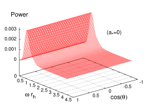
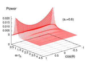
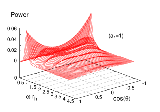
Figure 10: Angular distribution of the power spectra for gauge boson emission from rotating black holes, for $n=1$ and $a_{*}=(0,0.6,1)$.

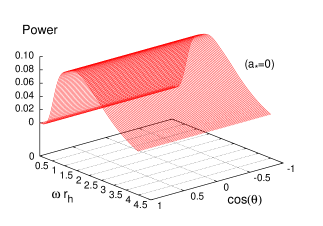
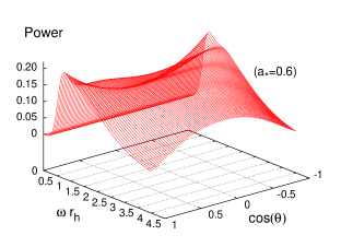
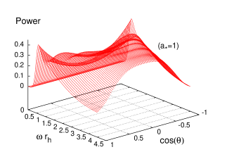
Figure 11: Angular distribution of the power spectra for gauge boson emission from rotating black holes, for $n=6$ and $a_{*}=(0,0.6,1)$.

The angular distribution of the power spectra for gauge boson emission on the brane is shown in Figs. 10 and 11, for the cases of $n=1$ and $n=6$, respectively, and for $a_{*}=(0,0.6,1)$. The same features exhibited by the flux spectra appear also here: the angular variation – absent for $a_{*}=0$ – makes its appearance in the spectrum as soon as the angular momentum parameter acquires non-zero values. Again, the low-energy emission channel runs parallel to the rotation axis, while, for higher-energies, the emission concentrates in the equatorial region. The amount of energy emitted per unit time and frequency along the equatorial plane increases also with the angular momentum parameter and the dimensionality of spacetime.

We should note here that our spectra are symmetric under the change $\theta\rightarrow\pi-\theta$, contrary to what was found in [21]; the difference is due to the fact that, in our analysis, both polarisations of the gauge field have been taken into account. Although, the two polarisations may have a different coupling with the black hole rotation, these couplings are both reversed when moving from one hemisphere to the other, thus resulting in a symmetric spectrum [30].

\psfrag{x}[0.8]{$\omega\,r_{\text{h}}$}\psfrag{y}[0.8]{$r_{\text{h}}\,d^{2}J/dt\,d\omega$}\includegraphics[height=142.26378pt,clip]{angs1n1.eps}      \psfrag{x}[0.8]{$\omega\,r_{\text{h}}$}\psfrag{y}[0.8]{$r_{\text{h}}\,d^{2}J/dt\,d\omega$}\includegraphics[height=142.26378pt,clip]{angs1n6.eps}

Figure 12: Angular momentum spectra for spin-1 particles from a rotating black hole, for (a) $n=1$, and (b) $n=6$, and various values of $a_{*}$.             

5.4 Angular momentum spectra

The final emission rate that we would like to study is the one of the angular momentum of the black hole. This differential rate, per unit time and unit frequency, is first shown in Figs. 12(a,b) for $n=1$ and $n=6$, respectively, and for variable $a_{*}$. Its behaviour is very similar to the one exhibited by the power emission spectrum. For $n=1$, the process of the angular momentum loss takes place predominantly through the emission of low-energy gauge particles, although the emission of particles with higher energy is still substantial. For $n=6$, on the other hand, the black hole loses its angular momentum through a more democratic process of emission, with a slight preference towards the emission of high-energy particles.

Figure 13 depicts the dependence of the angular momentum loss rate on the dimensionality of spacetime, while fixing the angular momentum parameter at $a_{*}=1$. As in the previous two cases of flux and power spectra, this rate is greatly enhanced, as the dimensionality of spacetime increases. The exact amount of the enhancement of the total angular momentum emissivity – which, as we will see, can reach more than an order of magnitude – will be discussed in the next subsection.

\psfrag{x}[0.8]{$\omega\,r_{\text{h}}$}\psfrag{y}[0.8]{$r_{\text{h}}^{2}\,d^{2}J/dt\,d\omega$}\includegraphics[height=156.49014pt,clip]{angs1a1.eps}

Figure 13: Angular momentum spectra for spin-1 particles from a rotating black hole, for $a_{*}=1$ and various values of $n$.             

5.5 Total emissivities

The total emissivities follow by integrating the various differential emission rates over the frequency regime, and give the total emission rate by the black hole per unit time. In principle, the integration over the frequency must cover all regimes in which the black hole radiates. However, deriving the whole Gaussian emission curve, as the angular momentum parameter and dimensionality of spacetime increase, soon becomes an unrealistic task. By looking, for instance, at Figs. 5, 9 and 13, one may easily see that while, for low values of $n$, all emission curves have been completed by the time the value of the energy parameter $\omega r_{h}=4$ is reached, for high values of $n$, the emission curves are still very close to their peak value. As both $a_{*}$ and $n$ take larger values, more and more high-energy particles are emitted by the black hole, and the tail of the curve extends to values of $\omega r_{h}$ much larger than the cutoff value of 4, up to which the radial part of the equation of motion of the gauge field has been numerically solved. Extending our energy regime towards much larger values has proved to be an extremely time-consuming process, therefore, in what follows, we will derive the “total emissivities” by integrating the emission rates up to our chosen cutoff value. As is obvious from the results presented in the previous subsections, an increase in the two fundamental parameters ($a_{*}$ and $n$) leads to a significant enhancement of the emission rates over the whole energy regime; the high-energy regime left out of our computation of the total emissivities, for large values of $a_{*}$ and $n$, would only increase further this enhancement. Therefore, the “total emissivities” derived, and presented in this subsection, can be considered as robust lower bounds to the exact ones.

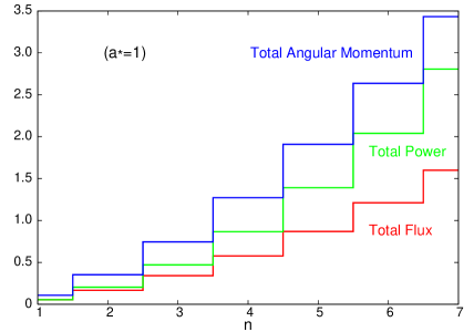
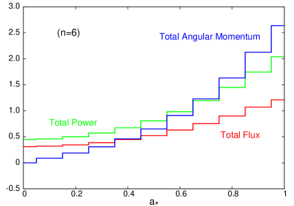
Figure 14: Total emissivities for spin-1 particle emission on the brane from a rotating black hole as a function of (a) $n$, for $a_{*}=1$, and (b) $a_{*}$, for $n=6$.

By following the above method, we have computed the total emissivities for the flux, power and angular momentum emitted by a higher-dimensional, rotating black hole on the brane in the form of gauge fields. The results, for fixed angular momentum parameter ($a_{*}=1$) and dimensionality ($n=6$), are depicted in the two histograms in Figs. 14(a) and (b), respectively. The enhancement of all three emissivities, that was foreseen while commenting on the results derived in the previous subsections, can be clearly observed. In the first histogram, the value of the number of additional spacelike dimensions $n$ varies from 1 to 7. A simple calculation shows that the number of particles emitted per unit time by a 11-dimensional, rotating (with $a_{*}=1$) black hole is 30 times larger than for a 5-dimensional one. Similarly, the total amount of energy emitted per unit time and the angular momentum loss rate for a 11-dimensional black hole are more than 50 and 30 times, respectively, larger than for a 5-dimensional black hole with the same angular velocity. For the reason explained in the beginning of this subsection, we expect these numbers to increase considerably when the high-energy part of the spectrum, for $n=7$, is included in the calculation.

The second histogram in Fig. 14 depicts the enhancement of the three emissivities when the dimensionality of spacetime is kept fixed (at $n=6$) and the angular momentum parameter varies. The data, used to produce this plot, reveal that the number of particles and amount of energy emitted by a 10-dimensional black hole with $a_{*}=1$ is 4 and 5 times, respectively, larger than the ones for a 10-dimensional, non-rotating black hole. As, in the case of $n=6$, a substantial part of the spectrum has been left out of the computation of the total emissivities, the aforementioned numbers should be treated as lower bounds only, with the exact numbers expected to reach values greater than these by even orders of magnitude. This can be deduced from the fact that, in the case of $n=1$, where all parts of the spectrum have been successfully derived and thus included in the computation of the exact total emissivities, the number of particles and amount of energy emitted per unit time by the 5-dimensional black hole with $a_{*}=1$ is already 10 and 15 times, respectively, larger than for its non-rotating, 5-dimensional analogue.

From the first histogram in Fig. 14, we observe that the emission rate of angular momentum remains always larger than the energy emission rate, with the former becoming increasingly larger than the latter as $n$ increases. This seems to support the argument that, during its decay, the angular momentum of a higher-dimensional black hole will be radiated away faster than its mass, thus signalling the existence of a subsequent non-rotating phase in the life of the black hole. Nevertheless, the second histogram in Fig. 14 shows that, for fixed dimensionality, the angular momentum emission rate strongly depends on the angular momentum of the black hole: while this rate is again significantly larger than the energy emission rate for rapidly rotating black holes, it is significantly smaller for slowly rotating ones. We might, thus, conclude that the evolution of rotating black holes goes through two different back-to-back stages: an initial one, where the black hole loses predominantly rotational kinetic energy, and a second one, where the – now slowly – rotating black hole loses mainly its mass. The exact duration of the two phases, as well as of the subsequent non-rotating one – if existent, will strongly depend on the initial angular momentum of the black hole and the dimensionality of spacetime.

We finally present the integral over the frequency of the angular distribution of the power spectrum (36) to derive the emissivity solely as a function of the azimuthal angle $\theta$. This is depicted in Figs. 15(a,b), as a function of $\cos\theta$ for fixed $n$ and variable $a_{*}$, and vice versa. As noted before, the shape of the angular distribution pattern is formed under the effect of the spin-rotation coupling and the centrifugal force, with the former dominating for low $a_{*}$ and low $n$, and the latter dominating for high $a_{*}$ and high $n$. The two symmetric peaks, due to the spin-rotation coupling, around $\cos\theta=\pm 1$ cannot be seen in Figs. 15 due to their very small magnitude – they barely survive the integration over the frequency due to the very small energies to which they correspond. Nevertheless, the aforementioned balance between the two competing forces leads to the type of distributions shown in Figs. 15, where a twin-peak pattern is formed. The derived shape of the integral over the frequency of the angular distribution of the power spectrum agrees with the corresponding one derived in the case of a 4-dimensional, rotating black hole [30].

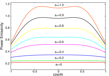
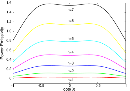
Figure 15: Power emissivity for spin-1 emission on the brane from a rotating black hole as a function of $\cos\theta$, (a) for $n=6$ and variable $a_{*}$, and (b) for $a_{*}=1$ and variable $n$.

5.6 Superradiance

In this final subsection, we address the issue of superradiance [59], i.e. the amplification of the amplitude of an incident bosonic wave by a rotating black hole. This takes place when the transmission coefficient becomes negative over a particular energy regime, i.e. when $\omega-m\Omega<0$, thus allowing for values of the reflection coefficient, defined as $\mathbb{R}_{\ell m\omega}=1-\mathbb{T}_{\ell m\omega}$, larger than unity. As noted in section 5.1, this behaviour coincides with the denominator in the expressions for the various fluxes (32)-(34) becoming also negative, therefore the Hawking radiation emission rates for these modes remain positive. The superradiance effect is known to take place in the pure 4-dimensional case for scalars, gauge bosons and gravitons [38, 59, 60]. In the case of a higher-dimensional black hole, the superradiance effect associated with either bulk [20] or brane [22, 23, 25] scalar fields has also been investigated. In [22], this effect was studied in detail in terms of both the dimensionality of spacetime and the angular momentum of the black hole. It was found that the energy amplification of 0.3% for scalars, for a 4-dimensional maximally rotating black hole with $a_{*}\simeq 1$ [60], increased by more than an order of magnitude for a 6-dimensional black hole, with the same angular momentum, emitting scalar fields on the brane. The amplification reached its highest value for the maximum values of both $n$ and $a_{*}$ considered in that work, namely $n=6$ and $a_{*}=4$, and it was found to be around 9%.

     

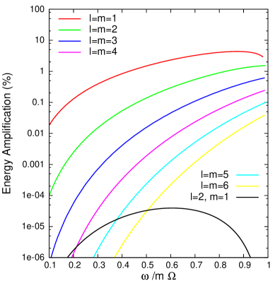
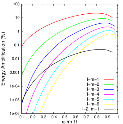
Figure 16: (a) Superradiant scattering of gauge bosons by a maximally rotating ($a=0.99999M_{BH}$) 4-dimensional black hole; (b) Super-radiant scattering of gauge bosons on the brane by an 11-dimensional black hole with $a_{*}=1$.                  

By following the conventions of Ref. [38], in Figs. 16(a) and (b), we depict the energy amplification of spin-1 fields due to the superradiance effect, for the cases of $n=0$ and $a_{*}=0.9955$, and $n=7$ and $a_{*}=1$, respectively. The vertical axis in these plots is minus the transmission coefficient, $-\mathbb{T}_{\ell m\omega}$, expressed as a percentage. The horizontal axis is the frequency interval over which $\mathbb{T}_{\ell m\omega}$ is negative, divided by $m\Omega$ to make the superradiant regime (0,1) for all modes. Figure 16(a) shows excellent agreement with the results produced for $n=0$ and $a=0.99999M_{BH}$ in [38]: the maximum amplification occurs for $\ell=m=1$, at $\omega/\Omega=0.88$, and it has a magnitude of 4.4%. However, as the dimensionality of spacetime increases, even while the angular momentum remains the same, these numbers change considerably: according to the data plotted in Fig. 16(b), the maximum amplification occurs again for the mode $\ell=m=1$ but this is now at $\omega/\Omega\simeq 0.8$, and it reaches the figure of 21.7%. The behaviour found in section 5.1 – and depicted in Fig. 3(b) – can easily explain the enhancement with $n$ in the superradiance amplification: for $a_{*}$ fixed, the transmission coefficient $\mathbb{T}_{\ell m\omega}$ was found to take increasingly larger negative values in the superradiance energy regime, as $n$ increased, due to the increase in the height of the gravitational barrier.

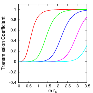
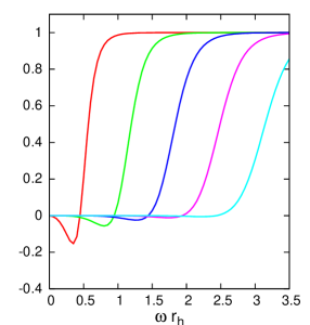
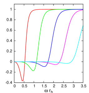
Figure 17: Transmission coefficients for spin-1 emission on the brane, for $n=6$, from a black hole with (a) $a_{*}=0$, (b) $a_{*}=0.9$, and (c) $a_{*}=1.2$. The curves, from left to right, correspond to the modes $\ell=m=1,2,3,4$, and 5.

As the superradiance effect is clearly associated with the rotation velocity of the black hole, we expect its magnitude to increase with the angular momentum parameter. Our findings in section 5.1 support this expectation as they clearly revealed the supression, with $a_{*}$, of the transmission coefficient, leading to increasingly larger negative values (see Fig. 2). Figure 17 depicts the behaviour of the transmission coefficient $\mathbb{T}_{\ell m\omega}$ for a whole set of spin-1 modes, for a 10-dimensional black hole ($n=6$) and various values of $a_{*}$. For the case of $a_{*}=0$, shown in Fig. 17(a), the transmission coefficient takes only positive values, and no superradiance occurs as expected. For $a_{*}=0.9$, shown in Fig. 17(b), the transmission coefficient does acquire negative values over a particular energy regime before it crosses the zero value and passes into the positive values regime: in this case, as it can be seen from the different curves, the maximum amplification takes place for $\ell=m=1$, and it amounts to 15.2%. As the angular momentum parameter increases further, the largest negative value of the transmission coefficient increases, too: for example, for the case of $a_{*}=1.2$, shown in Fig. 17(c), the superradiance amplification reaches the figure of 36.5%.

As $a_{*}$ and/or $n$ increase further, we expect the superradiance effect to become even more important. In an attempt to determine the maximum value of the energy amplification due to the superradiance, the extreme case of $n=7$ and $a_{*}=a^{\text{max}}_{*}=4.5$, as dictated by Eq. (7), was studied. Contrary to the case of the energy amplification of scalar fields [22], it was found that even for large values of $n$ and $a_{*}$, the lowest superradiant mode $\ell=m=1$ is still the dominant one. For this particular mode, it was found that the energy amplification reaches the amazing figure of 4200%, at $\omega/\Omega=0.84$.

6 Conclusions

The potential detection of Hawking radiation from a higher-dimensional black hole formed in the context of a brane-world model (either with Large Extra Dimensions [1], or warped extra dimensions [61] in the limit of $r_{h}\ll\ell_{AdS}$, with $\ell_{AdS}$ the AdS radius) demands the derivation of exact results for the various emission rates during both the spin-down and Schwarzschild phases in the life of the black hole. After the Schwarzschild phase was exhaustively studied, the spin-down phase eventually came into the foreground, with a few early and recent papers offering partial studies of the emission of Hawking radiation from a rotating brane-world black hole. The first complete study of the emission of scalar fields on the brane by such a black hole was performed only recently in [28]. The present paper complements and expands the latter one by focusing on the emission of gauge bosons from a $(4+n)$-dimensional rotating black hole on the brane – where the gauge bosons are restricted to live by assumption. A comprehensive analysis of the different emission rates, in terms of the values of the fundamental parameters of the model, was offered, and additional important aspects of physical processes associated with a rotating black hole, such as the angular distribution of the emitted particles and the superradiance effect, were also studied.

By generalizing techniques that were originally developed for the case of 4-dimensional black holes, to apply in the cases of higher-dimensional black hole line-elements projected onto a brane, we first derived the equation of motion for spin-1 particles propagating in the induced-on-the-brane gravitational background, and decoupled the radial and angular part (apart from the presence of the angular eigenvalue that appears in both parts thus linking them). We then proceeded to review, and generalize where necessary, the principles leading to the expressions of the transmission coefficient and of the various Hawking radiation emission fluxes. The calculation of the transmission coefficient demanded the numerical integration of the radial part of the equation of motion, while the angular distribution of the emitted particles demanded the numerical integration of the angular part - before, however, these two tasks could be performed, the exact value of the angular eigenvalue had to be computed, again numerically. Our numerical techniques were discussed in detail in Section 4.

In Section 5, we presented exact numerical results, first, for the transmission coefficient and, subsequently, for the particle, energy and angular momentum fluxes. The differential emission rates per unit time and frequency, integrated over the azimuthal angle $\theta$, were computed first, and their dependence on the dimensionality of spacetime, the angular momentum of the black hole and the energy of the emitted particle was investigated. It was demonstrated that all three emission rates were enhanced over the whole energy regime as the number of additional spacelike dimensions and the angular momentum of the black hole increase. In the case of the particle flux spectra, it was found that particles with a low energy are more likely to be emitted than particles with intermediate and high energy, however the emission of the latter ones becomes increasingly more significant as either $n$ or $a_{*}$ increase. In the case of power and angular-momentum emission spectra, for low values of $n$, both of these quantities are predominantly reduced through the emission of low-energy particles; as the dimensionality of spacetime takes larger values however, it is the intermediate and high-energy particles that carry away most of the energy and angular momentum of the black hole.

The angular distribution of the emitted particles and energy was also studied in detail. That became possible after the exact values of the spin-1 weighted spheroidal harmonics, valid for arbitrary values of the angular momentum of the black hole and energy of the emitted particle, were determined. The angular variation in the pattern of the emitted radiation can be a distinctive signature of emission from a rotating black hole, but also of the spin and energy of the particles emitted. In Figs. 18(a) and (b), we present for comparison the angular distribution of the energy emission spectrum for a 6-dimensional ($n=2$) rotating black hole emitting radiation on the brane, in the form of scalar and gauge particles, respectively. As expected, the uniform distribution of particles seen in the case of a non-rotating spherically-symmetric black hole is now replaced by a clearly oriented one, however the exact pattern is strongly dependent on both the spin and energy of the emitted particle. In the case of scalar particles [28], the centrifugal force exerted by the rotating black hole forces the scalar particles to concentrate on the equatorial plane ($\theta=0$); nevertheless, this angular variation disappears in the low energy part of the spectrum where the spherically-symmetric $\ell=m=0$ modes dominate, while it strongly appears in the intermediate and high-energy part of the spectrum where the non-spherically-symmetric modes become important. In the case of gauge particles, as we saw in this work, the angular distribution comes as the result of two forces: the centrifugal one, and the spin-rotation coupling due to the non-vanishing spin of the particle. It turns out that the latter one dominates for low-energy particles, forcing them to align parallel to the rotation axis ($\theta=\pm\pi$), while it becomes subdominant compared to the centrifugal force in the high-energy regime, causing the particles to concentrate again in the equatorial plane. A similar behaviour for the emission of gauge particles was seen also in the 4-dimensional case [30]; in the present case, it was found that the number of additional spacelike dimensions work towards enhancing further the centrifugal force.

     

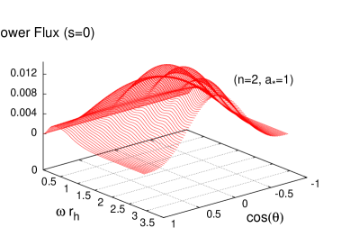
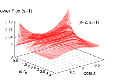
Figure 18: Angular distribution of the power spectra, for (a) scalar particle emission, and (b) gauge particle emission, from a 6-dimensional black hole with $a_{*}=1$ on the brane.

An important quantity associated to the emission of Hawking radiation from a black hole is the total emissivity, that describes the emission of either particles, energy or angular momentum per unit time, over the whole frequency band. In fact, in our analysis, lower bounds for the total emissivities were computed instead of the actual total ones, as the differential emission rates were integrated over the energy from zero to the chosen cut-off value of 4. This task was performed for all three emission rates, namely for the particle, energy and angular momentum fluxes. Their dependence on the azimuthal angle, the angular momentum of the black hole and the number of additional dimensions was investigated. In terms of the first quantity, both the particle and energy emissivities were found to have a twin-peak pattern under the influence of the centrifugal force and the spin-rotation coupling. In terms of the other two parameters, all emissivities were found to increase substantially as $n$ and $a_{*}$ increased; for instance, the energy emission per unit time increased 5-fold, for a 10-dimensional black hole, as $a_{*}$ increased from 0 to 1, and 50-fold, for a black hole with $a_{*}=1$, when $n$ increased from 1 to 7.

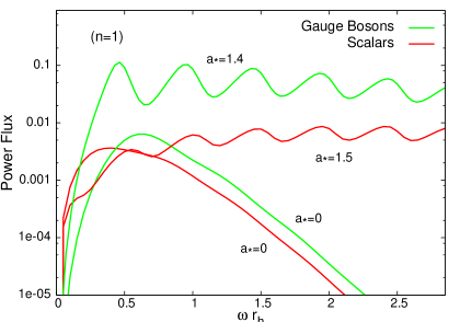
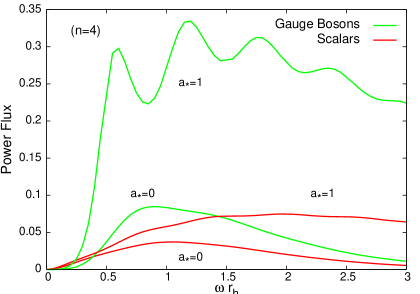
Figure 19: Energy emission rates for scalars and gauge bosons, for (a) $n=1$, and (b) $n=4$, and various values of $a_{*}$.

An interesting question that arises when one combines results on the various emission rates for different types of fields (i.e. scalars, gauge bosons and fermions) is which type of fields is preferably emitted by the black hole as both $n$ and $a_{*}$ vary. In the case of non-rotating black holes ($a_{*}=0$), it was found [7, 14] that a 4-dimensional black hole emits mainly scalar particles, a 6-dimensional black hole prefers a democratic distribution of particles, while the spectrum of a 10-dimensional black hole is dominated by gauge bosons. A similar behaviour is expected in the case of a rotating black hole. Looking at the vertical axes of Figs. 18(a,b), one can easily see that the emission rates for scalars and gauge bosons differ significantly, for the same values of $n$ and $a_{*}$. In order to investigate this in more detail, we have displayed in Figs. 19(a) and (b) the emission rates for scalars and gauge bosons, for fixed $n$ ($n=1$ and $n=4$, respectively), and for similar values of $a_{*}$. Figure 19(a) confirms the fact that for a non-rotating black hole living in a spacetime with a low value of $n$, the emission rate for gauge bosons becomes comparable to that of scalars only when both polarizations are included. When, however, the angular momentum of the black hole is turned on, the emission rate for gauge bosons becomes significantly larger than the one for scalar fields over the whole energy regime. Moving to the $n=4$ case, we see that indeed, for $a_{*}=0$, the gauge bosons already clearly dominate over the scalar fields; when the angular momentum is added on top, the increase becomes even larger. We may therefore conclude that a rotating black hole strongly prefers to emit gauge bosons over scalar particles for all values of $n$.

The final issue addressed in this work was the superradiance effect associated to the amplification of a bosonic wave incident on a rotating black hole. We have found that, in the case of gauge fields, similarly to the scalar case, this effect is present and greatly enhanced by the addition of extra spacelike dimensions transverse to the brane. The effect in this case is actually more important than in the scalar one: the superradiance effect increases from 4.4% to 21.7% as the dimensionality of spacetime goes from $D=4$ to $D=11$, even as the angular momentum of the black hole remains the same. Vice versa, for fixed dimensionality, i.e. $n=6$, the energy amplification varied from 0%, for $a_{*}=0$, as expected, to 36.5%, for $a_{*}=1.2$. As the superradiance effect is clearly augmented by both $n$ and $a_{*}$, the maximum energy amplification was sought by looking at the extreme case of $n=7$ and $a_{*}=a^{\text{max}}_{*}=4.5$: the lowest superradiant mode $\ell=m=1$ provided again the maximum amplification that was found to reach the amazing figure of 4200%.

The study of the emission of gauge fields on the brane by a higher-dimensional rotating black hole, performed in this work, has revealed a number of distinct features associated with the behaviour and magnitude of the different emission rates, the angular distribution of particles and energy, the relative enhancement compared to the scalar fields, and the magnitude of the superradiance effect. Apart from the theoretical interest in studying modifications of the properties of black holes submerged into a higher-dimensional space, we expect these features to comprise clear signatures of the emission of Hawking radiation of a brane-world black hole during its spin-down phase upon successful detection of this effect during an experiment. Having starting with the study of the emission of salar fields on the brane by such a black hole [28], we have offered in this work a similar, comprehensive analysis of the case of gauge fields; we hope to return soon with complete results for the emission of fermions that will eventually complete the study of the decay of a small, higher-dimensional rotating black hole through the emission of Standard Model fields on the brane.

Acknowledgments. We would like to thank Chris M. Harris for useful discussions. The work of P.K. is funded by the UK PPARC Research Grant PPA/A/S/2002/00350. The work of E.W. is supported by UK PPARC, grant reference number PPA/G/S/2003/ 00082, the Royal Society and the London Mathematical Society.

References

-
[1]
N. Arkani-Hamed, S. Dimopoulos and G. R. Dvali,
Phys. Lett. B 429, 263 (1998) [hep-ph/9803315];
Phys. Rev. D 59, 086004 (1999) [hep-ph/9807344];
I. Antoniadis, N. Arkani-Hamed, S. Dimopoulos and G. R. Dvali, Phys. Lett. B 436, 257 (1998) [hep-ph/9804398]. -
[2]
T. Banks and W. Fischler,
hep-th/9906038;
D. M. Eardley and S. B. Giddings, Phys. Rev. D 66, 044011 (2002) [gr-qc/0201034];
H. Yoshino and Y. Nambu, Phys. Rev. D 66, 065004 (2002) [gr-qc/0204060]; Phys. Rev. D 67, 024009 (2003) [gr-qc/0209003];
E. Kohlprath and G. Veneziano, JHEP 0206, 057 (2002) [gr-qc/0203093];
V. Cardoso, O. J. C. Dias and J. P. S. Lemos, Phys. Rev. D 67, 064026 (2003) [hep-th/0212168];
E. Berti, M. Cavaglia and L. Gualtieri, Phys. Rev. D 69, 124011 (2004) [hep-th/ 0309203];
V. S. Rychkov, Phys. Rev. D 70, 044003 (2004) [hep-ph/0401116];
S. B. Giddings and V. S. Rychkov, Phys. Rev. D 70, 104026 (2004) [hep-th/0409131];
O. I. Vasilenko, hep-th/0305067, hep-th/0407092;
H. Yoshino and V. S. Rychkov, Phys. Rev. D 71, 104028 (2005) [hep-th/0503171]. -
[3]
K. Akama,
Lect. Notes Phys. 176, 267 (1982) [hep-th/0001113];
V. A. Rubakov and M. E. Shaposhnikov, Phys. Lett. B 125, 139 (1983); Phys. Lett. B 125, 136 (1983);
M. Visser, Phys. Lett. B 159, 22 (1985) [hep-th/9910093];
G. W. Gibbons and D. L. Wiltshire, Nucl. Phys. B 287, 717 (1987);
I. Antoniadis, Phys. Lett. B 246, 377 (1990);
I. Antoniadis, K. Benakli and M. Quiros, Phys. Lett. B 331, 313 (1994) [hep-ph/9403290];
J. D. Lykken, Phys. Rev. D 54, 3693 (1996) [hep-th/9603133]. - [4] P. C. Argyres, S. Dimopoulos and J. March-Russell, Phys. Lett. B 441, 96 (1998) [hep-th/9808138].
-
[5]
S. B. Giddings and S. Thomas,
Phys. Rev. D 65, 056010 (2002) [hep-ph/0106219];
S. Dimopoulos and G. Landsberg, Phys. Rev. Lett. 87, 161602 (2001) [hep-ph/0106295];
S. Dimopoulos and R. Emparan, Phys. Lett. B 526, 393 (2002) [hep-ph/0108060];
S. Hossenfelder, S. Hofmann, M. Bleicher and H. Stocker, Phys. Rev. D 66, 101502 (2002) [hep-ph/0109085];
K. Cheung, Phys. Rev. Lett. 88, 221602 (2002) [hep-ph/0110163];
R. Casadio and B. Harms, Int. J. Mod. Phys. A 17, 4635 (2002) [hep-ph/0110255];
S. C. Park and H. S. Song, J. Korean Phys. Soc. 43, 30 (2003) [hep-ph/0111069];
G. Landsberg, Phys. Rev. Lett. 88, 181801 (2002) [hep-ph/0112061];
G. F. Giudice, R. Rattazzi and J. D. Wells, Nucl. Phys. B 630, 293 (2002) [hep-ph/0112161];
E. J. Ahn, M. Cavaglia and A. V. Olinto, Phys. Lett. B 551, 1 (2003)[hep-th/0201042];
T. G. Rizzo, JHEP 0202, 011 (2002) [hep-ph/0201228]; JHEP 0501, 025 (2005) [hep-ph/0412087];
A. V. Kotwal and C. Hays, Phys. Rev. D 66, 116005 (2002) [hep-ph/0206055];
A. Chamblin and G. C. Nayak, Phys. Rev. D 66, 091901 (2002) [hep-ph/0206060];
T. Han, G. D. Kribs and B. McElrath, Phys. Rev. Lett. 90, 031601 (2003) [hep-ph/0207003];
I. Mocioiu, Y. Nara and I. Sarcevic, Phys. Lett. B 557, 87 (2003) [hep-ph/0310073];
M. Cavaglia, S. Das and R. Maartens, Class. Quant. Grav. 20, L205 (2003) [hep-ph/0305223];
C. M. Harris, P. Richardson and B. R. Webber, JHEP 0308, 033 (2003) [hep-ph/0307305];
D. Stojkovic, Phys. Rev. Lett. 94, 011603 (2005) [hep-ph/0409124];
S. Hossenfelder, Mod. Phys. Lett. A 19, 2727 (2004) [hep-ph/0410122];
C. M. Harris, M. J. Palmer, M. A. Parker, P. Richardson, A. Sabetfakhri and B. R. Webber, JHEP 0505, 053 (2005) [hep-ph/0411022]. -
[6]
A. Goyal, A. Gupta and N. Mahajan,
Phys. Rev. D63, 043003 (2001) [hep-ph/0005030];
J. L. Feng and A. D. Shapere, Phys. Rev. Lett. 88, 021303 (2002) [hep-ph/0109106];
L. Anchordoqui and H. Goldberg, Phys. Rev. D65, 047502 (2002) [hep-ph/0109242];
R. Emparan, M. Masip and R. Rattazzi, Phys. Rev. D65, 064023 (2002) [hep-ph/ 0109287];
L. A. Anchordoqui, J. L. Feng, H. Goldberg and A. D. Shapere, Phys. Rev. D 65, 124027 (2002) [hep-ph/0112247]; Phys. Rev. D68, 104025 (2003) [hep-ph/0307228];
Y. Uehara, Prog. Theor. Phys. 107, 621 (2002) [hep-ph/0110382];
J. Alvarez-Muniz, J. L. Feng, F. Halzen, T. Han and D. Hooper, Phys. Rev. D 65, 124015 (2002) [hep-ph/0202081];
A. Ringwald and H. Tu, Phys. Lett. B 525, 135 (2002) [hep-ph/0111042];
M. Kowalski, A. Ringwald and H. Tu, Phys. Lett. B 529, 1 (2002) [hep-ph/0111042];
E. J. Ahn, M. Ave, M. Cavaglia and A. V. Olinto, Phys. Rev. D 68, 043004 (2003) [hep-ph/0306008];
E. J. Ahn, M. Cavaglia and A. V. Olinto, Astropart. Phys. 22, 377 (2005) [hep-ph/0312249];
T. Han and D. Hooper, New J. Phys. 6 (2004) 150 [hep-ph/0408348];
A. Cafarella, C. Coriano and T. N. Tomaras, JHEP 0506, 065 (2005) [hep-ph/0410358];
D. Stojkovic and G. D. Starkman, hep-ph/0505112;
A. Barrau, C. Feron and J. Grain, Astrophys. J. 630, 1015 (2005) [astro-ph/0505436];
L. Anchordoqui, T. Han, D. Hooper and S. Sarkar, hep-ph/0508312;
E. J. Ahn and M. Cavaglia, hep-ph/0511159. - [7] P. Kanti, Int. J. Mod. Phys. A 19, 4899 (2004) [hep-ph/0402168].
-
[8]
M. Cavaglia,
Int. J. Mod. Phys. A 18, 1843 (2003) [hep-ph/0210296];
G. Landsberg, Eur. Phys. J. C 33, S927 (2004) [hep-ex/0310034];
K. Cheung, hep-ph/0409028;
S. Hossenfelder, hep-ph/0412265;
A. S. Majumdar and N. Mukherjee, Int. J. Mod. Phys. D 14, 1095 (2005) [astro-ph/0503473]. - [9] C.M. Harris, hep-ph/0502005.
- [10] S. W. Hawking, Commun. Math. Phys. 43, 199 (1975).
- [11] P. Kanti and J. March-Russell, Phys. Rev. D 66, 024023 (2002) [hep-ph/0203223].
- [12] V. P. Frolov and D. Stojkovic, Phys. Rev. D 66, 084002 (2002) [hep-th/0206046].
- [13] P. Kanti and J. March-Russell, Phys. Rev. D 67, 104019 (2003) [hep-ph/0212199].
- [14] C. M. Harris and P. Kanti, JHEP 0310, 014 (2003) [hep-ph/0309054].
- [15] P. Kanti, J. Grain and A. Barrau, Phys. Rev. D 71, 104002 (2005) [hep-th/0501148].
-
[16]
A. Barrau, J. Grain and S. O. Alexeyev,
Phys. Lett. B 584, 114 (2004);
J. Grain, A. Barrau and P. Kanti, hep-th/0509128. - [17] E. l. Jung, S. H. Kim and D. K. Park, Phys. Lett. B 586, 390 (2004) [hep-th/0311036]; JHEP 0409, 005 (2004) [hep-th/0406117]; Phys. Lett. B 602, 105 (2004) [hep-th/0409145].
- [18] M. Doran and J. Jaeckel, astro-ph/0501437.
-
[19]
E. Jung and D. K. Park,
Nucl. Phys. B 717, 272 (2005) [hep-th/0502002];
E. Jung, S. Kim and D. K. Park, Phys. Lett. B 614, 78 (2005) [hep-th/0503027]. - [20] V. P. Frolov and D. Stojkovic, Phys. Rev. D 67, 084004 (2003) [gr-qc/0211055].
- [21] D. Ida, K. y. Oda and S. C. Park, Phys. Rev. D 67, 064025 (2003) [Erratum-ibid. D 69, 049901 (2004)] [hep-th/0212108].
- [22] C. M. Harris and P. Kanti, hep-th/0503010.
- [23] D. Ida, K. y. Oda and S. C. Park, Phys. Rev. D 71, 124039 (2005) [hep-th/0503052].
- [24] D. Ida, K. y. Oda and S. C. Park, hep-ph/0501210.
- [25] E. Jung, S. Kim and D. K. Park, Phys. Lett. B 615, 273 (2005) [hep-th/0503163]; Phys. Lett. B 619, 347 (2005) [hep-th/0504139].
- [26] H. Nomura, S. Yoshida, M. Tanabe and K. i. Maeda, Prog. Theor. Phys. 114, 707 (2005) [hep-th/0502179].
- [27] E. Jung and D. K. Park, hep-th/0506204.
- [28] G. Duffy, C. Harris, P. Kanti and E. Winstanley, JHEP 0509, 049 (2005) [hep-th/0507274].
- [29] R. C. Myers and M. J. Perry, Annals Phys. 172, 304 (1986).
- [30] M. Casals and A. C. Ottewill, Phys. Rev. D 71, 124016 (2005) [gr-qc/0501005].
- [31] S. A. Teukolsky, Phys. Rev. Lett. 29, 1114 (1972).
- [32] S. A. Teukolsky, Astrophys. J. 185, 635 (1973).
- [33] S. Chandrasekhar, The Mathematical Theory Of Black Holes (Oxford University Press, Oxford, 1992).
- [34] P. L. Chrzanowski, Phys. Rev. D 11, 2042 (1975).
- [35] P. L. Chrzanowski, R. A. Matzner, V. D. Sandberg and M. P. Ryan, Phys. Rev. D 14, 317 (1976).
- [36] J. M. Cohen and L. S. Kegeles, Phys. Rev. D 10, 1070 (1974).
- [37] R. M. Wald, Phys. Rev. Lett. 41, 203 (1978).
- [38] S. A. Teukolsky and W. H. Press, Astrophys. J. 193, 443 (1974).
- [39] E. Newman and R. Penrose, J. Math. Phys. 3, 566 (1962).
- [40] B. Carter, in B. Carter and J. B. Hartle, Gravitation In Astrophysics, Proceedings, Nato Advanced Study Institute, Cargese, France, July 15-31, 1986 (Plenum Press and NATO Scientific Affairs Division, New York, 1987).
- [41] R. H. Price, Phys. Rev. D 5, 2439 (1972).
- [42] M. Casals, Ph.D. thesis, University College Dublin (2004).
- [43] M. Casals and A. C. Ottewill, Phys. Rev. D 71, 064025 (2005) [gr-qc/0409012].
- [44] W. H. Press and S. A. Teukolsky, Astrophys. J. 185, 649 (1973).
- [45] A. A. Starobinskii and S. M. Churilov, Zh. Eksp. Teor. Fiz. 65, 3 (1973).
- [46] E. D. Fackerell and R. G. Grossman, J. Math. Phys. 18, 1849 (1977).
- [47] E. Seidel, Class. Quant. Grav. 6, 1057 (1989).
- [48] R. A. Breuer, Gravitational Perturbation Theory and Synchrotron Radiation, Lecture Notes in Physics Vol. 44 (Springer, Berlin, 1975).
- [49] R. Breuer, M. Ryan Jr. and S. Waller, Proc. R. Soc. London A 358, 71 (1977).
- [50] V. P. Frolov and K. S. Thorne, Phys. Rev. D 39, 2125 (1989).
- [51] S. M. Christensen, Phys. Rev. D 17, 946 (1978).
- [52] B. Jensen, J. McLaughlin and A. Ottewill, Class. Quant. Grav. 5, L187 (1988).
- [53] D. N. Page, Phys. Rev. D 14, 3260 (1976).
- [54] W. H. Press, S. A. Teukolsky, W. T. Vetterling and B. P. Flannery, Numerical Recipes in Fortran (Cambridge University Press, Cambridge, 2002).
- [55] S. L. Detweiler, Proc. R. Soc. London A 349, 217 (1976).
- [56] S. L. Detweiler, Proc. R. Soc. London A 352, 381 (1977).
- [57] M. Sasaki and T. Nakamura, Prog. Theor. Phys. 67, 1788 (1982).
- [58] R. M. Corless, G. H. Gonnet, D. E. Hare, D. J. Jeffrey and D. E. Knuth, Adv. Comp. Math. 5, 329 (1996).
- [59] Y.B. Zel’dovich, JETP Lett. 14, 180 (1971).
- [60] W. Press and S.A. Teukolsky, Nature 238, 211 (1972).
- [61] L. Randall and R. Sundrum, Phys. Rev. Lett. 83, 3370 (1999) [hep-ph/9905221]; Phys. Rev. Lett. 83, 4690 (1999) [hep-ph/9906064].