Effective Potential of QCD

Abstract

We present a simple method to calculate the one-loop effective action of QCD which reduces the calculation to that of $SU(2)$ QCD. For the chromomagnetic background we show that the effective potential has an absolute minimum only when two color magnetic fields $H_{\mu\nu}^{3}$ and $H_{\mu\nu}^{8}$ are orthogonal to each other. For the chromoelectric background we find that the imaginary part of the effective action has a negative signature, which implies the gluon pair-annihilation. We discuss the physical implications of our result.

I Introduction

An interesting problem which has been studied recently is to calculate the soft gluon production rate in a constant chromoelectric background nayak ; plb05 . This problem is closely related to the problem to calculate the QCD effective action in a constant chromoelectric background, because the imaginary part of the effective action determines the production rate schw ; prl01 . This leads to one of the most outstanding problems in theoretical physics, the problem to calculate the QCD effective action in an arbitrary homogeneous (constant) chromomagnetic and chromoelectric background, which has been studied by many authors savv ; niel ; yil ; adl ; sch ; prd02 ; jhep . The purpose of this Letter is to repeat the calculation with a different method, and to study the vacuum structure of the effective action.

For the chromomagnetic background we find that the effective potential has a non-trivial dependence on the relative space orientation of two magnetic fields $H_{\mu\nu}^{3}$ and $H_{\mu\nu}^{8}$. Given the fact that the classical potential depends only on $(H_{\mu\nu}^{3})^{2}+(H_{\mu\nu}^{8})^{2}$, this is surprising. More importantly, it has an absolute minimum only when they become orthogonal to each other. When they are parallel, the effective potential has two degenerate local minima. To the best of our knowledge, this constitutes a new evidence that a quantum fluctuation can actually determine the space orientation of a magnetic field. For the chromoelectric background we find that the imaginary part of the effective action become negative, which should be contrasted with known results yil ; sch .

To calculate the one-loop effective action one must decompose the gluon field into two parts, the slow-varying classical background $\vec{B}_{\mu}$ and the fluctuating quantum part $\vec{Q}_{\mu}$, and integrate the quantum part dewitt ; pesk . But this decomposition has to be gauge independent for the effective action to be gauge independent. A natural way to have a gauge independent decomposition is to make the Abelian projection. To make the Abelian projection we let $\hat{n}$ be the color octet unit vector which selects the color direction at each space-time point, and require cho1 ; cho2

$$D_{\mu}\hat{n}=0.~{}~{}~{}~{}~{}(\hat{n}^{2}=1)$$ (1)

This generates another constraint on the gauge potential

$$D_{\mu}\hat{n}^{\prime}=0,~{}~{}~{}\hat{n}^{\prime c}=\sqrt{3}d_{ab}^{~{}~{}c}\hat{n}^{a}\hat{n}^{b}.~{}~{}~{}(\hat{n}^{\prime 2}=1)$$ (2)

Notice that when $\hat{n}$ is $\lambda_{3}$-like, $\hat{n}^{\prime}$ becomes $\lambda_{8}$-like, so that one may always choose $\hat{n}$ to be a $\lambda_{3}$-like $\hat{n}_{3}$ and $\hat{n}^{\prime}$ a $\lambda_{8}$-like $\hat{n}_{8}$. The Abelian projection uniquely determine the restricted potential, the most general Abelian gauge potential $\hat{A}_{\mu}$, in QCD

$$\hat{A}_{\mu}=\sum_{p}\Big{(}A_{\mu}^{i}\hat{n}_{i}-\displaystyle\frac{1}{g}\hat{n}_{i}\times\partial_{\mu}\hat{n}_{i}\Big{)}.~{}~{}~{}(i=3,8)$$ (3)

where $A_{\mu}^{i}=\hat{n}_{i}\cdot\vec{A}_{\mu}$ are the chromoelectric potentials. With this the most general QCD potential is written as

$$\vec{A}_{\mu}=\hat{A}_{\mu}+{\vec{X}}_{\mu},~{}~{}~{}\hat{n_{i}}\cdot\vec{X}_{\mu}=0,~{}~{}~{}(i=3,8)$$ (4)

where ${\vec{X}}_{\mu}$ is the valence potential.

The decomposition (4) allows two types of gauge transformation, the background gauge transformation described by

$$\delta\hat{A}_{\mu}=\displaystyle\frac{1}{g}{\hat{D}}_{\mu}{\vec{\alpha}},~{}~{}~{}~{}~{}\delta{\vec{X}}_{\mu}=-{\vec{\alpha}}\times{\vec{X}}_{\mu},$$ (5)

and the quantum gauge transformation described by

$$\delta\hat{A}_{\mu}=0,~{}~{}~{}~{}~{} \delta{\vec{X}}_{\mu}=\displaystyle\frac{1}{g}{\hat{D}}_{\mu}{\vec{\alpha}}.$$ (6)

The background gauge transformation shows that $\hat{A}_{\mu}$ by itself enjoys the full $SU(3)$ gauge degrees of freedom, even though it describes the Abelian part of the potential. Furthermore $\vec{X}_{\mu}$ transforms covariantly under (5), which is why we call it the valence potential. But what is most important is that the decomposition (4) is gauge-independent. Once the color direction $\hat{n}$ is selected, the decomposition follows automatically, independent of the choice of a gauge cho1 ; cho2 .

With the decomposition (4) one has

$$\vec{F}_{\mu\nu}=\hat{F}_{\mu\nu}+{\hat{D}}_{\mu}{\vec{X}}_{\nu}-{\hat{D}}_{\nu}{\vec{X}}_{\mu}+g{\vec{X}}_{\mu}\times{\vec{X}}_{\nu},$$

$$\hat{F}_{\mu\nu}=G_{\mu\nu}^{i}\hat{n}_{i},~{}~{}~{}~{}~{}G_{\mu\nu}^{i}=F_{\mu\nu}^{i}+H_{\mu\nu}^{i}$$

$$F_{\mu\nu}^{i}=\partial_{\mu}A_{\nu}^{i}-\partial_{\nu}A_{\mu}^{i},$$

$$H_{\mu\nu}^{i}=-\displaystyle\frac{1}{g}\hat{n}_{i}\cdot(\partial_{\mu}\hat{n}_{i}\times\partial_{\nu}\hat{n}_{i})=\partial_{\mu}C_{\nu}^{i}-\partial_{\nu}C_{\mu}^{i},$$ (7)

where $C_{\mu}^{i}$ is the chromomagnetic potentials. This tells that restricted potential has a dual structure. With (7) the QCD Lagrangian can be written as follows

$${\cal L}=-\displaystyle\frac{1}{4}{\hat{F}}_{\mu\nu}^{2}-\displaystyle\frac{1}{4}({\hat{D}}_{\mu}{\vec{X}}_{\nu}-{\hat{D}}_{\nu}{\vec{X}}_{\mu})^{2}$$

$$-\displaystyle\frac{g}{2}{\hat{F}}_{\mu\nu}\cdot({\vec{X}}_{\mu}\times{\vec{X}}_{\nu})-\displaystyle\frac{g^{2}}{4}({\vec{X}}_{\mu}\times{\vec{X}}_{\nu})^{2}.$$ (8)

This shows that QCD is a restricted gauge theory which has a gauge covariant valence gluon as a colored source.

With this we can integrate the quantum field $\vec{X}_{\mu}$ with the gauge fixing $\hat{D}_{\mu}\vec{X}_{\mu}=0$. For this we first introduce three complex vector fields ($W_{\mu}^{p},~{}p=1,2,3$ )

$$W^{1}_{\mu}=\displaystyle\frac{1}{\sqrt{2}}(X_{\mu}^{1}+iX_{\mu}^{2}),~{}~{}~{}W^{2}_{\mu}=\displaystyle\frac{1}{\sqrt{2}}(X_{\mu}^{6}+iX_{\mu}^{7}),~{}~{}~{}W^{3}_{\mu}=\displaystyle\frac{1}{\sqrt{2}}(X_{\mu}^{4}-iX_{\mu}^{5}),$$ (9)

and express the QCD Lagrangian as

$${\cal L}=-\displaystyle\frac{1}{6}\sum_{p}({\cal G}_{\mu\nu}^{p})^{2}+\displaystyle\frac{1}{2}\sum_{p}|D_{p\mu}W_{\nu}^{p}-D_{p\nu}W_{\mu}^{p}|^{2}+ig\sum_{p}{\cal G}_{\mu\nu}^{p}W_{\mu}^{p*}W_{\nu}^{p}-\displaystyle\frac{1}{2}g^{2}\sum_{p}\big{[}(W_{\mu}^{p*}W_{\mu}^{p})^{2}-(W_{\mu}^{p*})^{2}(W_{\nu}^{p})^{2}\big{]},$$

$${\cal G}_{\mu\nu}^{p}=\partial_{\mu}{\cal B}_{\nu}^{p}-\partial_{\nu}{\cal B}_{\mu}^{p},~{}~{}~{}~{}~{}D_{p\mu}W_{\nu}^{p}=(\partial_{\mu}+ig{\cal B}_{\mu}^{p})W_{\nu}^{p},$$

$${\cal B}_{\mu}^{1}=B_{\mu}^{3},~{}~{}~{}{\cal B}_{\mu}^{2}=-\displaystyle\frac{1}{2}B_{\mu}^{3}+\displaystyle\frac{\sqrt{3}}{2}B_{\mu}^{8},~{}~{}~{}{\cal B}_{\mu}^{3}=-\displaystyle\frac{1}{2}B_{\mu}^{3}-\displaystyle\frac{\sqrt{3}}{2}B_{\mu}^{8},~{}~{}~{}B_{\mu}^{i}=A_{\mu}^{i}+C_{\mu}^{i},$$ (10)

Notice that the potentials ${\cal B}_{\mu}^{p}$ are precisely the dual potentials in $i$-spin, $u$-spin, and $v$-spin direction in color space which couple to three valence gluons $W_{\mu}^{p}$. With this we have the following integral expression of the one-loop effective action

$$\exp\Big{[}iS_{eff}(\hat{A}_{\mu})\Big{]}=\displaystyle\frac{}{}\sum_{p}\int{\cal D}W_{\mu}{\cal D}W_{\mu}^{*}{\cal D}c_{1}{\cal D}c_{1}^{\dagger}{\cal D}c_{2}{\cal D}c_{2}^{\dagger}\exp\Big{\{}\displaystyle\frac{}{}i\int\Big{[}-\displaystyle\frac{1}{6}{\cal G}_{\mu\nu}^{2}-\displaystyle\frac{1}{2}|{D}_{\mu}{W}_{\nu}-{D}_{\nu}{W}_{\mu}|^{2}$$

$$+ig{\cal G}_{\mu\nu}W_{\mu}^{*}W_{\nu}-\displaystyle\frac{1}{2}g^{2}\Big{[}(W_{\mu}^{*}W_{\mu})^{2}-(W_{\mu}^{*})^{2}(W_{\nu})^{2}\Big{]}-\displaystyle\frac{1}{\xi}|{D}_{\mu}W_{\mu}|^{2}$$

$$+c_{1}^{\dagger}({D}^{2}+g^{2}W_{\mu}^{*}W_{\mu})c_{1}-g^{2}c_{1}^{\dagger}W_{\mu}W_{\mu}c_{2}+c_{2}^{\dagger}({D}^{2}+g^{2}W_{\mu}^{*}W_{\mu})^{*}c_{2}-g^{2}c_{2}^{\dagger}W^{*}_{\mu}W^{*}_{\mu}c_{1}~{}\Big{]}d^{4}x\Big{\}},$$ (11)

where $\vec{c}$ and ${\vec{c}}^{~{}*}$ are the ghost fields. Notice that here we have suppressed the summation index $p$ in the integrand. Now a few remarks are in order. First, notice that except for the $p$-summation the integral expression is identical to that of $SU(2)$ QCD prd02 ; jhep . This shows that one can reduce the calculation of QCD effective action to that of $SU(2)$ QCD. Secondly, the above result can easily be generalized to $SU(N)$ QCD with $N(N-1)/2$ $p$-summation. Thirdy, one might include the Abelian part in the functional integration, but this does not affect the result because the Abelian part has no self-interaction. This tells that only the valence gluon loops contribute to the integration. Finally, the bakground $\hat{F}_{\mu\nu}$ can still have a non-trivial fluctuation, because $\hat{n}_{3}$ and $\hat{n}_{8}$ have an arbitrary space-time dependence. Only ${\cal G}_{\mu\nu}$ need be constant cho3 .

Now, from the $SU(2)$ QCD result we have prd02 ; jhep

$$\Delta S=i\sum_{p}\ln{\rm Det}(-D_{p}^{2}+2gH_{p})(-D_{p}^{2}-2gH_{p})+i\sum_{p}\ln{\rm Det}(-D_{p}^{2}-2igE_{p})(-D_{p}^{2}+2igE_{p})-2i\sum_{p}\ln{\rm Det}(-D_{p}^{2}),$$

$$H_{p}=\displaystyle\frac{1}{2}\sqrt{\sqrt{{\cal G}_{p}^{4}+({\cal G}_{p}\tilde{\cal G}_{p})^{2}}+{\cal G}_{p}^{2}},~{}~{}~{}~{}~{}E_{p}=\displaystyle\frac{1}{2}\sqrt{\sqrt{{\cal G}_{p}^{4}+({\cal G}_{p}\tilde{\cal G}_{p})^{2}}-{\cal G}_{p}^{2}},$$ (12)

from which we obtain

$$\Delta{\cal L}=\lim_{\epsilon\rightarrow 0}\displaystyle\frac{g^{2}}{16\pi^{2}}\sum_{p}\int_{0}^{\infty}\displaystyle\frac{dt}{t^{3-\epsilon}}\displaystyle\frac{H_{p}E_{p}t^{2}}{\sinh(gH_{p}t/\mu^{2})\sin(gE_{p}t/\mu^{2})}\Big{[}\exp(-2gH_{p}t/\mu^{2})+\exp(+2gH_{p}t/\mu^{2})$$

$$+\exp(+2igE_{p}t/\mu^{2})+\exp(-2igE_{p}t/\mu^{2})-2\Big{]}.$$ (13)

Notice that for the magnetic background we have $E_{p}=0$, but for the electric background we have $H_{p}=0$.

The evaluation of the funtional integral is straightforward. But it has the well-known infra-red divergence which has to be regularized, and the funtional integration depends on the regularization method savv ; niel ; yil ; adl ; sch ; prd02 ; jhep . Consider the magnetic background first. With the $\zeta$-function regularization we obtain niel ; prd02 ; jhep ; cho3

$${\cal L}_{eff}=-\sum_{p}\Big{(}\displaystyle\frac{H_{p}^{2}}{3}+\displaystyle\frac{11g^{2}}{48\pi^{2}}H_{p}^{2}(\ln\displaystyle\frac{gH_{p}}{\mu^{2}}-c)$$

$$+i\displaystyle\frac{g^{2}}{8\pi}H_{p}^{2}\Big{)}.$$ (14)

But if we adopt the gauge invariant regularization which respects the causality, we find that the effective action has the same real part, but no imaginary part sch ; prd02 ; jhep ; cho3

As for the electric background we find, using the $\zeta$-function regularization prd02 ; jhep ; cho3 ,

$${\cal L}_{eff}=\sum_{p}\Big{(}\displaystyle\frac{E_{p}^{2}}{3}+\displaystyle\frac{11g^{2}}{48\pi^{2}}E_{p}^{2}(\ln\displaystyle\frac{gE_{p}}{\mu^{2}}-c)$$

$$-i\displaystyle\frac{23g^{2}}{96\pi}E_{p}^{2}\Big{)}.$$ (15)

But with the gauge invariant regularization we find that the imaginary part changes to sch ; prd02 ; jhep ; cho3

$$Im~{}{\cal L}_{eff}=-\sum_{p}\displaystyle\frac{11g^{2}}{96\pi}E_{p}^{2}.$$ (16)

Notice that, independent of the regularization method, the imaginary part has a negative signature. This might look strange, because this implies a negative probability of gluon pair-creation. But we notice that the negative signature is a direct consequence of the Bose-statistics of the gluon loop.

The effective action has a manifest Weyl symmetry, the six-element subgroup of $SU(3)$ which contains the cyclic $Z_{3}$. Furthermore it has the dual symmetry. It is invariant under the dual transformation $H_{p}\rightarrow-iE_{p}$ and $E_{p}\rightarrow iH_{p}$. Notice that this is exactly the same dual symmetry which we have in QED and $SU(2)$ QCD prl01 ; prd02 . We can also express the effective actions (14) and (15) in terms of three Casimir invariants, $(\hat{F}_{\mu\nu}^{a})^{2}$, $(d_{bc}^{~{}~{}a}\hat{F}_{\mu\nu}^{b}\hat{F}_{\mu\nu}^{c})^{2}$, and $(d_{abc}\hat{F}_{\mu\nu}^{a}\hat{F}_{\nu\rho}^{b}\hat{F}_{\rho\sigma}^{c})^{2}$, replacing $H_{p}$ (and $E_{p}$) by the Casimir invariants, which assures the gauge invariance of the effective actions. But it should be noticed that the imaginary part of the effective actions depend only on one Casimir invariant, $(\hat{F}_{\mu\nu}^{a})^{2}$.

Just as in $SU(2)$ QCD we can obtain the effective potential from the effective action. For the constant magnetic background the effective potential is given by

$$V_{eff}=\displaystyle\frac{1}{2}(\bar{H}_{3}^{2}+\bar{H}_{8}^{2})+\displaystyle\frac{11g^{2}}{48\pi^{2}}\Big{\{}\bar{H}_{3}^{2}\ln\big{(}\displaystyle\frac{g\bar{H}_{3}}{\mu^{2}}-c\big{)}$$

$$+\bar{H}_{+}^{2}\ln\big{(}\displaystyle\frac{g\bar{H}_{+}}{\mu^{2}}-c\big{)}+\bar{H}_{-}^{2}\ln\big{(}\displaystyle\frac{g\bar{H}_{-}}{\mu^{2}}-c\big{)},$$

$$\bar{H}_{\pm}^{2}=\displaystyle\frac{1}{4}\bar{H}_{3}^{2}+\displaystyle\frac{3}{4}\bar{H}_{8}^{2}\pm\displaystyle\frac{\sqrt{3}}{2}\bar{H}_{3}\bar{H}_{8}\cos\theta,$$

$$\bar{H}_{3}=\sqrt{(H_{\mu\nu}^{3})^{2}/2},~{}~{}~{}\bar{H}_{8}=\sqrt{(H_{\mu\nu}^{8})^{2}/2},$$

$$\cos\theta=H_{\mu\nu}^{3}H_{\mu\nu}^{8}/2\bar{H}_{3}\bar{H}_{8}.$$ (17)

Notice that the classical potential depends only on $\bar{H}_{3}^{2}+\bar{H}_{8}^{2}$, but the effective potential depends on three variables $\bar{H}_{3}$, $\bar{H}_{8}$, and $\cos\theta$. At first thought this might look strange, but as we have remarked this is because the effective action depends on three invariant variables, which can be chosen to be $\bar{H}_{3}$, $\bar{H}_{8}$, and $\cos\theta$. We emphasize that $\cos\theta$ can be arbitrary because $H_{\mu\nu}^{3}$ and $H_{\mu\nu}^{8}$ are completely independent, so that they can have different space polarization. The potential has the unique minimum at $\bar{H}_{3}=\bar{H}_{8}=H_{0}$ and $\cos\theta=0$. Notice that when $H_{\mu\nu}^{3}$ and $H_{\mu\nu}^{8}$ are parallel (or when $\cos\theta=1$) it has two degenerate minima at $\bar{H}_{3}=\tilde{H}_{0},~{}\bar{H}_{8}=0$ and at $\bar{H}_{3}=\tilde{H}_{0}/2,~{}\bar{H}_{8}=\sqrt{3}\tilde{H}_{0}/2$, where $\tilde{H}_{0}=\root 1/3 \of{2}~{}H_{0}$. We plot the effective potential for $\cos\theta=1$ in Fig. 1 and for $\cos\theta=0$ in Fig. 2 for comparison.

One can renormalize the potential by defining a running coupling $\bar{g}^{2}(\bar{\mu}^{2})$

$$\displaystyle\frac{\partial^{2}V_{eff}}{\partial\bar{H}_{i}^{2}}\Big{|}_{\bar{H}_{3}=\bar{H}_{8}=\bar{\mu}^{2},\theta=\pi/2}=\displaystyle\frac{g^{2}}{\bar{g}^{2}}$$

$$=1+\displaystyle\frac{11}{16\pi^{2}}g^{2}(\ln\displaystyle\frac{\bar{\mu}^{2}}{\mu^{2}}-c+\displaystyle\frac{5}{4}),~{}~{}~{}~{}(i=3,8)$$ (18)

from which we retrieve the QCD $\beta$-function

$$\beta(\bar{\mu})=\bar{\mu}\displaystyle\frac{d\bar{g}}{d\bar{\mu}}=-\displaystyle\frac{11}{16\pi^{2}}\bar{g}^{3}.$$ (19)

The renormalized potential has the same form as in (17), with the replacement $g\rightarrow\bar{g},~{}\mu\rightarrow\bar{\mu},~{}c=5/4$. It has the unique minimum

$$V_{min}=-\displaystyle\frac{11\bar{\mu}^{4}}{32\pi^{2}}\exp\big{(}-\displaystyle\frac{32\pi^{2}}{11\bar{g}^{2}}+\displaystyle\frac{3}{2}\big{)},$$

$$<\bar{H}_{3}>=<\bar{H}_{8}>=\displaystyle\frac{\bar{\mu}^{2}}{\bar{g}}\exp\big{(}-\displaystyle\frac{16\pi^{2}}{11\bar{g}^{2}}+\displaystyle\frac{3}{4}\big{)}.$$ (20)

It should be noticed that the effective potential breaks the original $SO(2)$ invariance (of $\bar{H}_{3}^{2}+\bar{H}_{8}^{2}$) of the classical Lagrangian.

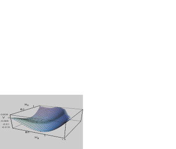
Figure 1: The QCD effective potential with $\cos\theta=1$, which has two degenerate minima.

The QCD effective action has been calculated before with different methods yil ; adl . Our method has the advantage that it naturally reduces the calculation of $SU(N)$ QCD effective action to that of $SU(2)$ QCD.

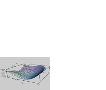
Figure 2: The effective potential with $\cos\theta=0$, which has a unique minimum at $\bar{H}_{3}=\bar{H}_{8}=H_{0}$.

There have been a lot of controversies and confusions on the imaginary part of the effective action niel ; yil ; adl ; sch ; prd02 ; jhep . This is (at least partly) due to the fact that the imaginary part depends on the regularization method. Here we remark that there is a straightforward way to resolve this controversy. Notice that the imaginary part depends only on the second order in coupling constant $g$. This implies that one can calculate the imaginary part independently from the perturbative Feynman diagram sch ; jhep . We find that the perturbative calculation supports the gauge invariant regularization.

Independent of this controversy we emphasize that in both regularizations the chromoelectric background generates a negative imaginary part. Only the quarks, due to the Fermi-statistics, has a positive contribution to the imaginary part. This should be contrasted with earlier results yil ; sch . The detailed discussion of the subject will be published elsewhere cho3 .

Acknowledgements

One of the authors (DGP) thanks N. Kochelev and P. M. Zhang for useful discussions. The work is supported in part by the ABRL Program of Korea Science and Engineering Foundation (R14-2003-012-01002-0) and by the BK21 Project of the Ministry of Education.

References

• (1) G. C. Nayak and P. van Nieuwenhuizen, Phys.Rev. D71 (2005) 125001; B. Muller, nucl-th/0508062.
• (2) Y. M. Cho, Phys. Lett. B616, 101 (2005).
• (3) J. Schwinger, Phys. Rev. 82, 664 (1951).
• (4) Y. M. Cho and D. G. Pak, Phys. Rev. Lett. 86, 1947 (2001); 91, 039101 (2003); W. S. Bae, Y. M. Cho, and D. G. Pak, Phys. Rev. D64, 017303 (2001).
• (5) G. K. Savvidy, Phys. Lett. B71, 133 (1977); S. G. Matinyan and G. K. Savvidy, Nucl. Phys. B134, 539 (1978).
• (6) N. K. Nielsen and P. Olesen, Nucl. Phys. B144, 376 (1978); Nucl. Phys. B160, 380 (1979).
• (7) A. Yildiz and P. Cox, Phys. Rev. D21, 1095 (1980).
• (8) S. Adler, Phys. Rev. D23, 2905 (1981); W. Dittrich and M. Reuter, Phys. Lett. B128, 321, (1983); I. Avramidi, J. Math. Phys. 36, 1557 (1995).
• (9) V. Schanbacher, Phys. Rev. D26, 489 (1982).
• (10) Y. M. Cho, H. W. Lee, and D. G. Pak, Phys. Lett. B 525, 347 (2002); Y. M. Cho and D. G. Pak, Phys. Rev. D65, 074027 (2002).
• (11) Y. M. Cho, D. G. Pak, and M. Walker, JHEP 05, 073 (2004); Y. M. Cho and M. L. Walker, Mod. Phys. Lett. A19, 2707 (2004); Y. M. Cho, hep-th/0301013.
• (12) B. de Witt, Phys. Rev. 162, 1195 (1967); 1239 (1967).
• (13) See for example, C. Itzikson and J. Zuber, Quantum Field Theory (McGraw-Hill) 1985; M. Peskin and D. Schroeder, An Introduction to Quantum Field Theory (Addison-Wesley) 1995; S. Weinberg, Quantum Theory of Fields (Cambridge Univ. Press) 1996.
• (14) Y. M. Cho, Phys. Rev. D21, 1080 (1980); Phys. Rev. D62, 074009 (2000).
• (15) Y. M. Cho, Phys. Rev. Lett. 46, 302 (1981); Phys. Rev. D23, 2415 (1981); W. S. Bae, Y. M. Cho, and S. W. Kimm, Phys. Rev. D65, 025005 (2002).
• (16) Y. M. Cho, J. H. Kim, and D. G. Pak, to be published.