hep-th/0511117 LMU-ASC 62/05 TIFR/TH/05-09
Non-Supersymmetric Attractors in String Theory

Abstract

We find examples of non-supersymmetric attractors in Type II string theory compactified on a Calabi Yau three-fold. For a non-supersymmetric attractor the fixed values to which the moduli are drawn at the horizon must minimise an effective potential. For Type IIA at large volume, we consider a configuration carrying D0, D2, D4 and D6 brane charge. When the D6 brane charge is zero, we find for some range of the other charges, that a non-supersymmetric attractor solution exists. When the D6 brane charge is non-zero, we find for some range of charges, a supersymmetry breaking extremum of the effective potential. Closer examination reveals though that it is not a minimum of the effective potential and hence the corresponding black hole solution is not an attractor. Away from large volume, we consider the specific case of the quintic in $CP^{4}$. Working in the mirror IIB description we find non-supersymmetric attractors near the Gepner point.

1 Introduction and Overview

Extremal black holes are known to exhibit an interesting phenomenon called the attractor mechanism. Moduli fields in these black holes are drawn to fixed values at the horizon. These fixed values are independent of the asymptotic values for the moduli and are determined entirely by the charges of the black hole. So far the attractor mechanism has been mainly discussed in the context of supersymmetric BPS states. It was first discovered in [1], has been studied quite extensively since then, [2, 3, 4, 5, 6, 7, 8], and has gained considerable attention lately due to the conjecture of [9] and related developments [10, 11, 12, 13, 14, 15, 16, 17, 18, 19]. More recently, it was shown that non-supersymmetric extremal black holes can also exhibit the attractor phenomenon [16, 21]. For some earlier related discussion see also [6, 20] and especially [5]. For BPS black holes in ${\cal N}=2$ supersymmetric theories it is known that the attractor values minimise the central charge [3]. More generally, for supersymmetric and non-supersymmetric extremal black holes, it was found that the attractor behavior can be understood in terms of an effective potential which depends on the charges and the moduli. The fixed values for the moduli are obtained by extremising this potential with respect to the moduli and the condition for an attractor is that the resultant extremum is a minimum.

In this paper we study examples of non-supersymmetric attractors in string theory. The setting is ${\cal N}=2$ supersymmetric compactifications of Type II string theory on a Calabi-Yau manifold . We are interested in extremal but non-supersymmetric black holes in these compactifications. And in this paper we focus on “big ” black holes with non-zero horizon area classically.

The discussion is structured as follows. We begin in Section 2, by briefly summarising some of the general formalism required, with reference in particular to the effective potential mentioned above. For an ${\cal N}=2$ theory the effective potential only involves the vector multiplet moduli, and can be obtained from the vector multiplet moduli space prepotential and the charges carried by the black hole. In the cases we encounter in this paper the second derivative matrix of the effective potential has some zero eigenvalues. In these situations higher corrections to the effective potential, beyond quadratic order, need to be calculated around the extremum. We show that the condition for an attractor is that the extremum is a minimum once these corrections are included.

Next, in Section 3, we turn to the specific case of Type II on Calabi-Yau manifolds. In the Type IIA description the vector multiplet moduli arise from the (complexified) Kahler moduli of the Calabi-Yau manifold. Working self-consistently at large volume, we analyse configurations carrying D6, D4, D2 and D0 brane charge. In the analysis we first consider the case where no D6 branes are present. In this case we find that for an appropriate ranges of charges a non-supersymmetric attractor exists.

Next we consider the case with D6 brane charge. Here we find that for an appropriate range of charges, an extremum of the effective potential exists and the resulting extremal Reissner Nordstrom black hole, obtained by setting the moduli fields at infinity equal to their extremum values, breaks supersymmetry. However, the effective potential is not a minimum in this case and so the black hole is not an attractor. It turns out that the second derivative matrix of the effective potential has some zero eigenvalues and the leading corrections to the effective potential is cubic along these directions in moduli space. This means that generic small deviations in the moduli at infinity do not die away near the horizon. Instead, they grow taking the solution further away from the extremal black hole as the horizon is approached.

We have not carried out an analysis of other possible extrema of the effective potential in the case with D6 brane charge. This could reveal the existence of a non-supersymmetric attractor. It could also be that the non-supersymmetric attractor configuration is a multi-centered black hole [8]. We leave a more complete investigation along these lines for the future.

An important comment about the non-supersymmetric black holes we have analysed is worth making here. The extremum value of the effective potential gives the Beckenstein-Hawking entropy of the black hole. One can also compute their entropy from a microscopic point of view. For the black holes without any D6 brane charge this can be done using the results of [22]. One finds that the microscopic entropy agrees with the Beckenstein-Hawking entropy. With D6 brane charge turned on the microscopic counting can be done for the case of $K3\times T^{2}$, as discussed in [23, 24, 25]. Once again one finds that the result matches the Beckenstein-Hawking entropy. This agreement between the microscopic counting and the Beckenstein-Hawking entropy for non-supersymmetric extremal black holes is truly striking. Note that with D6 brane charge turned on the black hole is not an attractor, as mentioned above. Even so the microscopic and macroscopic answers agree. The agreement of entropy for non-supersymmetric extremal black holes has been noticed before, [24, 25, 26, 27, 28, 29]. We hope to develop a better understanding for this phenomenon in a forthcoming paper [30].

In Section 4, we consider an example away from the large volume limit of the Calabi-Yau manifold. Generally speaking the analysis is more difficult now, since the effective potential is harder to construct explicitly. One other limit which can sometimes be analysed analytically is that of small complex structure in the mirror IIB description. We illustrate this in the case of the mirror quintic. The period integrals in this region of moduli space can be obtained by a power series expansion. This allows the effective potential to be constructed explicitly. By adjusting the charges we find examples of non-supersymmetric attractors where the moduli are fixed self-consistently in the vicinity of Gepner point. It would be interesting to carry out a microscopic counting of the entropy in these cases also to compare with the gravity answer. A similar analysis can be easily repeated for other Calabi-Yau manifolds. Examples with few moduli, or where the charges are turned on in a symmetric way so that the minimum lies in a symmetric subspace of the moduli space would be most tractable.

2 Brief Introduction to Non-Supersymmetric Attractors

2.1 Brief Introduction

In this subsection we briefly review the results of [21], see also [16].

We consider a theory whose bosonic terms have the form,

$$S=\frac{1}{\kappa^{2}}\int d^{4}x\sqrt{-G}(R-2g_{ij}(\partial\phi^{i})(\partial\phi^{j})-f_{ab}(\phi_{i})F^{a}_{\mu\nu}F^{b\ \mu\nu}-{\textstyle{1\over 2}}{\tilde{f}}_{ab}(\phi_{i})F^{a}_{\mu\nu}F^{b}_{\rho\sigma}\epsilon^{\mu\nu\rho\sigma}).$$ (1)

$F^{a}_{\mu\nu},a=0,\cdots N$ are gauge fields. $\phi^{i},i=1,\cdots n$ are scalar fields. The scalars have no potential term but determine the gauge coupling constants. We note that $g_{ij}$ refers to the metric in the moduli space. This is different from the spacetime metric $g_{\mu\nu}$.

A spherically symmetric space-time metric in $3+1$ dimensions takes the form,

$$ds^{2} = -a(r)^{2}dt^{2}+a(r)^{-2}dr^{2}+b(r)^{2}d\Omega^{2}$$ (2)

The Bianchi identity and equation of motion for the gauge fields can be solved by a field strength of the form,

$$F^{a}=f^{ab}(\phi_{i})(Q_{eb}-{\tilde{f}}_{bc}Q^{c}_{m}){1\over b^{2}}dt\wedge dr+Q_{m}^{a}sin\theta d\theta\wedge d\phi,$$ (3)

where $Q_{m}^{a},Q_{ea}$ are constants that determine the magnetic and electric charges carried by the gauge field $F^{a}$, and $f^{ab}$ is the inverse of $f_{ab}$.

The effective potential $V_{eff}$ is then given by,

$$V_{eff}(\phi_{i})=f^{ab}(Q_{ea}-{\tilde{f}}_{ac}Q^{c}_{m})(Q_{eb}-{\tilde{f}}_{bd}Q^{d}_{m})+f_{ab}Q^{a}_{m}Q^{b}_{m}.$$ (4)

It follows from the Lagrangian, eq.(1), and the metric, eq.(2), that the scalar fields satisfy the equation,

$$\partial_{r}(a^{2}b^{2}g_{ij}\partial_{r}\phi^{j})=\frac{\partial_{i}V_{eff}}{2b^{2}}.$$ (5)

And the metric components satisfy the relations,

$$(a^{2}(r)b^{2}(r))^{{}^{\prime\prime}} = 2,$$ (6)

$$\frac{b^{{}^{\prime\prime}}}{b} = -g_{ij}\partial_{r}\phi^{i}\partial_{r}\phi^{j}.$$ (7)

For the attractor mechanism it is sufficient for two conditions to be met. First, for fixed charges, as a function of the moduli, $V_{eff}$ must have a critical point. Denoting the critical values for the scalars as $\phi^{i}=\phi^{i}_{0}$ we have,

$$\partial_{i}V_{eff}(\phi_{i0})=0.$$ (8)

Second, the matrix of second derivatives of the potential at the critical point,

$$M_{ij}={1\over 2}\partial_{i}\partial_{j}V_{eff}(\phi_{i0})$$ (9)

should have positive eigenvalues. Schematically we can write,

$$M_{ij}>0.$$ (10)

We will sometimes refer to $M_{ij}$ as the mass matrix and it’s eigenvalues as masses (more correctly $mass^{2}$ terms) for the fields, $\phi_{i}$.

Once the two conditions mentioned above are met it was argued in [21] that the attractor mechanism works. There is an extremal Reissner Nordstrom black hole solution in the theory, where the black hole carries the charges specified by the parameters, $Q^{a}_{m},Q_{ea},$ and the moduli take the critical values, $\phi_{i0}$, at infinity. For small deviations of the moduli from these values at infinity a double-zero horizon extremal black hole solution continues to exist. In this extremal black hole the scalars take the same fixed values, $\phi_{0}$, at the horizon independent of their values at infinity. The resulting horizon radius is given by,

$$b_{H}^{2}=V_{eff}(\phi_{i0})$$ (11)

and the entropy is

$$S_{BH}={1\over 4}A=\pi b_{H}^{2}.$$ (12)

In this paper we will encounter situations where some of the eigenvalues of $M_{ij}$ vanish. The leading correction to $V_{eff}$ along a zero-eigenmode direction is then not quadratic but a higher power of the field. Two cases will be encountered, in these the leading power is quartic and cubic respectively. We show below that as long as the quartic term is positive, there is attractor behaviour. In contrast, in the cubic case there is no attractor behaviour. More generally for attractor behavior the leading correction to the effective potential must be positive. We turn to an analysis of these situations next.

2.2 Vanishing Mass terms and Attractors

We begin by considering a case where one eigenvalue of $M_{ij}$, eq.(9), vanishes. We denote the corresponding eigenmode by $\phi$ below. The leading correction to $V(\phi)$ along the $\phi$ direction is then a polynomial,

$$V(\phi) = V(\phi_{0})+\lambda(\delta\phi)^{n}$$ (13)

$$\delta\phi = \phi-\phi_{0}.$$ (14)

Our analysis will be along the lines of [21]. We start with an extremal Reissner Nordstrom (eRN) black hole, with the scalar fields fixed at their extremum values, and look at small perturbations. The perturbations satisfy second order equations. The essential point is that if one of the two solutions of the scalar perturbation equation is well behaved, and vanishes, in the vicinity of the horizon, then one has attractor behavior. This is because at infinity the effects of the electromagnetic flux vanish and both solutions to the perturbation equation are acceptable. Thus, starting with the good solution near the horizon one can extend it to infinity in a smooth fashion.

In the vicinity of the horizon, $r=r_{H}$, the metric of the ERN black hole takes the form,

$$ds^{2}=-{(r-r_{H})^{2}\over r_{H}^{2}}dt^{2}+{r_{H}^{2}\over(r-r_{H})^{2}}dr^{2}+r^{2}d\Omega^{2}.$$ (15)

It is useful to define a coordinate $t$ given by,

$$e^{-t}\equiv{r-r_{H}\over r_{H}}.$$ (16)

Note that $t\rightarrow\infty$, as $(r-r_{H})\rightarrow 0$.

Let us first consider the case where the eigenvalue of $M_{ij}$ is non vanishing, and $V(\phi)=V(\phi_{0})+{1\over 2}m^{2}(\delta\phi)^{2}$. From eq.(5) the equation for $\delta\phi$ now takes the form ,

$${\delta{\ddot{\phi}}}-{\delta{\dot{\phi}}}-{m^{2}\over r_{H}^{2}}{\delta\phi}=0.$$ (17)

This corresponds to a particle moving in an upside down harmonic oscillator potential with an anti-friction force that aids in its motion. The attractor solutions correspond to a one parameter family in which $\delta\phi$ reaches the origin of the potential asymptotically, as $t\rightarrow\infty$. The approach is exponential in $t$, $\delta\phi=Ae^{-\alpha t}$, where, $\alpha$ is determined by the mass,

$$\alpha={-1+\sqrt{1+4{m^{2}\over r_{H}^{2}}}\over 2}.$$ (18)

Now turn to the case where the mass term vanishes and the leading correction to the potential is quartic,

$$V(\phi)=V(\phi_{0})+\lambda(\delta\phi)^{4}.$$ (19)

For $\lambda>0$ one can see that there is a one parameter family of solutions, which is the analogue of the slow roll solution in inflation, in which the particle moves due to the anti-friction force driving it up the hill, with the second derivative term being small. This takes the form,

$$(\delta\phi)^{2}={r_{H}^{2}\over 8\lambda(t+c)},$$ (20)

where $c$ is the constant that specifies the one parameter family. Note that $(\delta\phi)\rightarrow 0$, as $t\rightarrow\infty$, so the attractor value is obtained at the horizon, but the approach is exponentially slower than in the case with non-vanishing mass.

At next order in the perturbation the backreaction on the metric can be calculated. One finds, for the metric, eq.(2), using eq.(6), eq.(7), that,

$$b = b_{0}+{r_{H}^{3}\over 64\lambda}{1\over t^{2}}+\cdots$$ (21)

$$a^{2} = a_{0}^{2}(1-{r_{H}^{2}\over 32\lambda}{1\over t^{2}})+\cdots,$$ (22)

where $a_{0}^{2}={(r-r_{H})^{2}\over r_{H}^{2}},b_{0}=r_{H},$ denote the zeroth order near-horizon metric components, eq.(15), and the ellipses indicate terms which are further suppressed in powers of $1/t$. Since $a_{0}$ has a double -zero at the horizon, we see from eq.(22) that after including the backreaction the metric continues to be a double-zero extremal black hole and from eq.(21) we see that the value of the radius $b$ approaches $r_{H}$ at the horizon.

So far we have analysed the attractor behavior in the vicinity of the horizon. Extending this analysis to asymptotic infinity is non-trivial in view of the non-linearity introduced by the quartic term, eq.(19). We have carried out such an analysis numerically and present the results in figure 1. As one might expect the well behaved attractor solution in the vicinity of the horizon matches smoothly to an asymptotically flat solution at infinity.

A similar near-horizon analysis can be repeated in the case where the potential takes the form, eq.(13), where $n$ is now a general even power greater than $2$. This leads to the conclusion mentioned above that the attractor mechanism works as long as $\lambda>0$ so that the attractor value is a minimum of $V_{eff}$.

In the discussion above we have neglected the mixing between the eigenmode $\phi$ and other massive directions in field space. In general such terms will arise when the potential is expanded about the extremum. However, in the vicinity of the horizon the massive eigenmodes will vanish exponentially more rapidly and such couplings can be neglected.

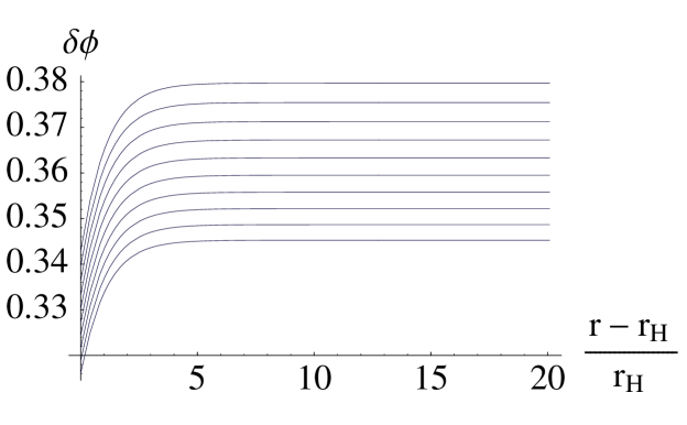
Figure 1: Plot for the field $\delta\phi\left({r-r_{H}\over r_{H}}\right)$ as a function of $\left({r-r_{H}\over r_{H}}\right)$ for different values of $c$. Here we have chosen $\lambda=1$ and $r_{H}=2$. The integration constant $c$ takes values $0.1,0.2\cdots 1.0$. The solution is interpolated from ${r-r_{H}\over r_{H}}=e^{-50}$ to ${r-r_{H}\over r_{H}}=e^{3}$.

Next, let us consider the case when the power $n$, eq.(13), is odd. For concreteness we take the case when $n=3,\lambda>0$. The equation now takes the form,

$${\delta{\ddot{\phi}}}-{\delta{\dot{\phi}}}-V_{eff}^{\prime}(\delta\phi)=0.$$ (23)

As in earlier cases the second term corresponds to an anti-friction force while the third term corresponds to a ”inverted potential” of the form, $V=-\lambda\phi^{3}$. It is now easy to see that a small perturbation in the near horizon region, with $\delta\phi<0$, does not die away. Instead, with ${\delta{\dot{\phi}}}>0$, both the anti-friction force and the potential drive the perturbation in the same direction towards $\delta\phi\rightarrow 0$. As a result the perturbation reaches $\delta\phi=0$ at finite $t$ and then continues to grow towards $\delta\phi\rightarrow\infty$ as $t\rightarrow\infty$. Once the perturbation becomes large enough the backreaction also becomes significant and our linearised approximation breaks down. We have not analysed in full detail the subsequent evolution. It seems reasonable to speculate that in general there is no non-singular black hole solution for such a perturbation. Thus we conclude that for the case where $n=3$ there is no attractor behaviour. It is straightforward to see that more generally a similar conclusion holds for all odd powers of $n$.

A succinct way to summarise our conclusions so far is the following: there is attractor behaviour only if the effective potential is a positive function of $\delta\phi$.

So far we have considered the case with one zero-eigenvalue of $M_{ij}$. In the situations we will encounter below there are mutiple zero-eigenvalues. One can show that our conclusions above apply in this more general case as well. Namely, that attractor behaviour only holds for a positive effective potential. Let us briefly sketch the argument here.

An equation of the form, eq.(23), now governs each of the zero-eigenmodes. If the effective potential is positive, a slow-roll solution can be shown to exist in which the second derivative term in eq.(23) is negligible and the second term due to anti-friction balances the gradient term from the potential. In this solution each zero-eigenmode relaxes to the attractor value as $t\rightarrow\infty$. However, if the effective potential is not positive such a solution does not exist in general. For appropriately chosen initial values of $\delta\phi_{i}$ the anti-friction term and the gradient of the potential point in the same direction. As a result along some directions $\delta\phi_{i}$ vanishes at finite $t$ and then continues to increase in magnitude in an unbounded manner till back reaction effects become important.

Two specific situations with zero-eigenvalues will arise in this paper. For Type IIA theory at large volume, without $D6$ brane charge, we will find a positive quartic potential with mutiple zero-eigenvalues in general. Once D6-brane charge is included we will find generically a cubic potential again with multiple zero-eigenvalues. From the discussion above we conclude that there will be attractor behaviour only in the first case.

2.3 ${\cal N}=2$ Theories

We conclude this section with a brief discussion of ${\cal N}=2$ supersymmetric theories. In these theories, $V_{eff}$ can be expressed, [5], in terms of a Kahler potential, $K$ and a superpotential, $W$ as,

$$V_{eff}=e^{K}[g^{i\bar{j}}\nabla_{i}W(\nabla_{j}W)^{*}+|W|^{2}],$$ (24)

where $\nabla_{i}W\equiv\partial_{i}W+\partial_{i}KW$.

The scalars which enter in $V_{eff}$ belong to vector multiplets and can be described in terms of special geometry. Special coordinates, $X^{a},a=0,\cdots N$, can be chosen to describe the $N$ dimensional space. The Kahler potential and superpotential which appear in eq.(24) can be expressed in terms of a prepotential $F$ which is a homogeneous holomorphic function of degree two in these coordinates. The Kahler potential is given by,

$$K=-\ln Im(\sum_{a=0}^{N}X^{a*}\partial_{a}F(X))$$ (25)

And the superpotential by,

$$W=\sum_{a=0}^{N}q_{a}X^{a}-p^{a}\partial_{a}F.$$ (26)

Note that in this notation, $q_{a}$ and $p^{a}$ are the parameters, $Q_{ea}$ and $Q_{m}^{a}$ respectively, eq.(3), which determine the electric and magnetic charges of the black hole.

For a BPS black hole, the central charge given by,

$$Z=e^{K/2}W,$$ (27)

is minimised, i.e., $\nabla_{i}Z=\partial_{i}Z+{1\over 2}\partial_{i}KZ=0$. This condition is equivalent to,

$$\nabla_{i}W=0.$$ (28)

The resulting entropy is given by

$$S_{BH}=\pi e^{K}|W|^{2}.$$ (29)

with the Kahler potential and superpotential evaluated at the attractor values.

It is worth noting here that in the supersymmetric case, when the central charge is minimised, [3], both terms on the r.h.s of eq.(24) are separately minimised. Since the central charge is minimised, the second term in eq.(24), $|Z|^{2}$, is at a minimum, and since this condition means that $\nabla W$ vanishes the first term in eq.(24) is also at a minimum. In contrast, for the non-supersymmetric black hole only their sum, $V_{eff}$ is minimised. In particular the central charge is not minimised in the non-supersymmetric case.

3 Type IIA at large Volume

In this section we analyse black hole attractors in Type IIA compactifications where the volume of the Calabi Yau manifold is large. The Calabi-Yau manifold we consider has $h(1,1)=N$. The resulting ${\cal N}=2$ low-energy theory has $N$ vector multiplets, and $N+1$ gauge fields. The one additional gauge field is the graviphoton which lies in the gravity multiplet. The leading order prepotential, with no $\alpha^{{}^{\prime}}$ corrections, takes the form,

$$F=D_{abc}{X^{a}X^{b}X^{c}\over X^{0}}$$ (30)

where $a,b,c=1,\cdots N$. The intersection numbers $D_{ABC}$ are given by,

$$6D_{abc}=\int_{M}\alpha_{a}\wedge\alpha_{b}\wedge\alpha_{c},$$ (31)

where $M$ denotes the Calabi-Yau manifold and $\alpha_{a}$ are an integer basis for $H^{2}(M;{\bf Z})$.

Type IIA theory has D0, D2, D4 and D6 branes. D0 branes and D6 branes are electrically and magnetically charged with respect to the graviphoton. D2 branes and D4 branes are electrically and magnetically charged with respect to the remaining $N$ gauge fields. A general configuration carries charges $(q_{0},q_{a},p^{0},p^{a})$, with $a=1,\cdots N$. To be more specific, an integral basis for $H^{2}(M;{\bf Z})$, $\alpha_{a}$, was introduced above. Let $\Sigma^{a}$ be a basis of 4-cycles dual to $\alpha_{a}$. And let ${\hat{\Sigma}}_{a}$ be a basis of 2-cycles Poincare dual to $\Sigma^{a}$. Then a D4 brane wrapping the cycle $\Sigma^{a}$, would carry magnetic charge, $p^{a}$. Similarly a D2 brane wrapping the cycle ${\hat{\Sigma}}_{a}$ would carry electric charge $q_{a}$.

The special coordinates introduced in subsection 2.3 above correspond to complexified Kahler moduli of the Calabi-Yau manifold. In particular $J$- the Kahler two-form of the Calabi-Yau- satisfies the relation,

$$\int_{{\hat{\Sigma}}_{a}}J=Im({X^{a}\over X^{0}}).$$ (32)

The superpotential in supergravity for a general configuration carrying charges, $(q_{0},q_{a},p^{0},p^{a})$, is given by, eq.(26).

In the discussion below, we first consider the case where the D6-brane charge is set to zero. Subsequently, we include D6 branes as well.

3.1 No D6 branes

Microscopically, the configuration we consider consists of a D4 brane wrapping the 4-cycle $[P]=p_{a}\Sigma^{a}$. In addition electric charges, $q_{0},q_{a}$ also arise due to gauge fields being turned on, on its world volume .

At large volume the prepotential is given by eq.(30). From eq.(26), with $p_{0}=0$, the superpotential takes the form,

$$W=q_{0}X^{0}+q_{a}X^{a}-3D_{abc}p^{a}{X^{b}X^{c}\over X^{0}}.$$ (33)

And from eq.(25) the Kahler potential is given by

$$K=-\ln\left(-iX^{0}{\bar{X}}^{0}D_{abc}\left({X^{a}\over X^{0}}-{{\bar{X}}^{a}\over{\bar{X}}^{0}}\right)\left({X^{b}\over X^{0}}-{{\bar{X}}^{b}\over{\bar{X}}^{0}}\right)\left({X^{c}\over X^{0}}-{{\bar{X}}^{c}\over{\bar{X}}^{0}}\right)\right)$$ (34)

The supersymmetric solution for this case are known [31, 32].

In the subsequent discussion we denote,

$$x^{a}=X^{a}/X^{0}$$ (35)

and work in the gauge $X^{0}=1$.

To begin it is also useful to first set $q_{a}=0$. Symmetries suggest the ansatz,

$$x^{a}=p^{a}t.$$ (36)

Then it is easy to see that the conditions, eq.(28), are solved by

$$t=i\sqrt{q_{0}/D},$$ (37)

where

$$D=D_{abc}p^{a}p^{b}p^{c}.$$ (38)

We also introduce for subsequent use the notation,

$$D_{ab}\equiv D_{abc}p^{c},D_{a}\equiv D_{abc}p^{b}p^{c}.$$ (39)

We are interested in non-supersymmetric solutions to the attractor conditions. As discussed in the previous section these must minimise the effective potential eq.(24). It is easy to see that this condition takes the form,

$$\partial_{a}V_{eff}=e^{K}\left(g^{b\bar{c}}\nabla_{a}\nabla_{b}W\overline{\nabla_{c}W}+2\nabla_{a}W\overline{W}+\partial_{a}g^{b\bar{c}}\nabla_{b}W\overline{\nabla_{c}W}\right)=0~{}.$$ (40)

Symmetries dictate that the ansatz eq.(36) must be good in this case as well. As discussed in appendix A.1, substituting for $x^{a}$ in terms of $t$ from eq.(36), eq.(40) takes the form,

$${6i\over t}(q_{0}-t^{2}D)(q_{0}+t^{2}D)=0$$ (41)

There are two non-singular solutions to eq.(41). The supersymmetric solution, eq.(37) is one of them. The second solution is non-supersymmetric and is given by,

$$t=i\sqrt{-q_{0}/D}$$ (42)

We note that a non-singular solution requires that the imaginary part of $t$ is non-vanishing (otherwise the volume of the Calabi-Yau vanishes) . Thus for a given set of charges we can either have a supersymmetric attractor or a non-supersymmetric attractor, depending on whether $q_{0}/D>0$ or $q_{0}/D<0$.

The entropy of the black hole is given by,

$$S=2\pi\sqrt{Dq_{0}},$$ (43)

in the supersymmetric case, and by

$$S=2\pi\sqrt{-Dq_{0}},$$ (44)

in the non-supersymmetric case. Note that the entropy in the non-supersymmetric case can be obtained from the supersymmetric case by analytically continuing in the charges.

So far we have set $q_{a}=0$. This condition is easily relaxed. The superpotential, in $X^{0}=1$ gauge takes the form,

$$W=(q_{0}+q_{a}x^{a}-3D_{bc}x^{b}x^{c})$$ (45)

Since it is quadratic in $x^{a}$ we can complete the square. Let us use the notation $D^{ab}$ for the inverse of the matrix, $D_{ab}$ introduced in eq.(39). Then, defining the variables,

$${\hat{q}}_{0} = q_{0}+{1\over 12}D^{ab}q_{a}q_{b}$$ (46)

$${\hat{x}}^{a} = x^{a}-{1\over 6}D^{ab}q_{b}$$ (47)

we find the Kahler potential and the superpotential take the same form in terms of the hatted variables as they did for the unhatted variables in the $q_{a}=0$ case above.

The solution in the supersymmetric and non-supersymmetric cases can then be easily written down and take the form,

$${\hat{x}}^{a}=ip^{a}\sqrt{{\hat{q}}_{0}\over D}$$ (48)

and,

$${\hat{x}}^{a}=ip^{a}\sqrt{-{\hat{q}}_{0}\over D}$$ (49)

respectively.

And the entropy in the two cases is given by

$$S=2\pi\sqrt{D{\hat{q}}_{0}},$$ (50)

and,

$$S=2\pi\sqrt{-D{\hat{q}}_{0}}.$$ (51)

Note that once again for any set of charges one has either the susy or the non-susy attractor but not both. One can go from the susy to the non-susy case by reversing the sign of some charges (for example, this can be done by taking $p^{a}\rightarrow-p^{a}$ keeping $q_{0},q_{a}$ fixed). And analytically continuing in the charges takes the entropy of the susy solution to the non-susy case.

We have worked in the large volume limit of Type IIA theory above. The volume $V$ is determined by the vector multiplet moduli in IIA theory and is therefore fixed by the attractor mechanism. For the solutions above it is given by $V\simeq|{q_{0}^{3}\over D}|^{1/2}$. By taking $q_{0}$ big enough we can make $V$ big. More generally we want the size of all two-cycles and 4-cycles to be big on the string scale. This leads to the condition, $Im(x^{a})>>1$. We see from eq.(37), eq.(42), that this condition can be met by taking $p^{a}\sqrt{|q_{0}/D|}>>1$. A similar condition can also be met by by adjusting the charges when $q_{a}\neq 0$ to ensure that the Calabi-Yau manifold has large volume.

It is also worth commenting that the ansatz, eq.(36), is singular if the charges $p^{a}$ are such that $D=D_{abc}p^{a}p^{b}p^{c}=0$. In this case the attractor value for the volume of the Calabi-Yau vanishes. In fact, this ansatz is inapplicable if $p^{a}=0$ for any value of the index $a$, since the volume of the corresponding 2-cycle, ${\hat{\Sigma}}_{a}$, vanishes.

Let us also comment on the physical meaning of the non-supersymmetric solutions we have found. We saw in eq.(43), eq.(44), that the non-supersymmetric solutions are obtained by say reversing the sign of $q_{0}$. Thus starting with a supersymmetric situation containing a D4 brane wrapped on a 4-cycle [P] with induced D0 brane charge $q_{0}$ such that $q_{0}/D>0$, we can get a non-supersymmertric configuration by changing the world volume fluxes on the brane so that the induced charge $q_{0}$ reverses sign. The solution we have found above is the supergravity description of this microscopic configuration. Similarly with $q_{a}$ charges also turned on once again changing the sign of the D0 brane charge leads to a non-supersymmetric configuration . It is worth commenting that since $|Dq_{0}|\gg 1$ for a big black hole, reversing the sign of $q_{0}$ leads to $O(1)$ breaking of supersymmetry.

So far we have ensured that the attractor values of the moduli extremise the effective potential. For an attractor $V_{eff}$ must be minimised. In the supersymmetric case this condition is automatically met, as was discussed in the previous section. In the non-supersymmetric case this needs to be verified by a direct calculation of the second derivatives at the extremum. We turn to this next.

3.2 The Matrix of Second Derivatives

There are $N$ vector multiplet moduli corresponding to $2N$ real scalars. As discussed in appendix B.1 the matrix of second derivatives at the non-susy extremum discussed above has $N+1$ positive eigen values and $N-1$ zero eigenvalues. These zero eigenvalues correspond to the following directions in moduli space.

Let us write

$$x^{a}=p^{a}t+\delta x^{a}$$ (52)

We see from eq.(49) that at the extremum, where $\delta x^{a}$ vanishes, $x^{a}$ is purely imaginary. The zero mass eigenmodes correspond to $\delta x^{a}$ being purely real and meeting the condition that

$$D_{abc}p^{b}p^{c}\delta x^{a}=0$$ (53)

To analyse the attractor behavior we need to expand the potential to higher orders in $\delta x^{a}$. It is enough for this purpose to only consider the zero eigenmodes, since the other direction have a positive second derivative. As discussed in appendix B.2 we get keeping terms upto quartic order that

$$V_{eff}=(V_{eff})_{0}+e^{K_{0}}\left[-72{q_{0}\over D}(D_{a}\delta x^{a})^{2}+36(D_{ab}\delta x^{a}\delta x^{b})^{2}\right]$$ (54)

where $(V_{eff})_{0},K_{0}$ are the values of the effective potential and the Kahler potential at the extremum.

Note that the quartic terms are positive. As discussed in section 2.2 this is enough to ensure that the solution is an attractor.

This completes our discussion of the Type IIA case with D0, D2 and D4 brane charges turned on. We turn to including D6 brane charge next.

The discussion above goes through essentially unchanged for the case when $q_{a}\neq 0$, by working in the hatted variables, introduced in eq.(46).

3.3 Adding D6 Branes

We now turn to adding $D6$ brane charge. The configuration we study has the following microscopic description. It consists of a single D6 brane wrapping the Calabi-Yau $p_{0}$ times. D4,D2 and D0 brane charges arise due to the world volume gauge field being turned on on its world volume (and also due to gravitational Chern-Simons terms). We will analyse the supergravity description of this configuration below. We find that once again depending on the charges there is either a supersymmetric or non-supersymmetric solution which extremises the effective potential. However, somewhat surprisingly, it will turn out that the non-supersymmetric solution is not an attractor. The mass matrix in this case has zero eigenvalues and the leading correction to the potential along these directions of field space is cubic in the perturbation, $\delta\phi$, eq.(176). For simplicity, throughout this subsection we restrict ourselves to the case where $q_{a}=0$.

The superpotential in $X^{0}=1$ gauge takes the form,

$$W=(q_{0}-3D_{ab}x^{a}x^{b}+p^{0}D_{abc}x^{a}x^{b}x^{c}).$$ (55)

The susy solution is known [32],

$$x^{a} = p^{a}t$$ (56)

$$t = {1\over 2D}\left(-p^{0}q_{0}\pm i\sqrt{q_{0}(4D-(p^{0})^{2}q_{0})}\right)$$ (57)

where

$$D=D_{abc}p^{a}p^{b}p^{c}$$ (58)

It has entropy,

$$S=\pi\sqrt{4Dq_{0}-(p^{0})^{2}q_{0}^{2}}.$$ (59)

The supersymmetric solution exists if

$${4D\over q_{0}}>(p^{0})^{2}.$$ (60)

Non-susy extrema of the effective potential $V_{eff}$ are described in appendix A.2. They exists when ${4D\over q_{0}}<(p^{0})^{2}$, i.e., when the inequality, eq.(60), is not met. These solutions are somewhat complicated. There are two branches depending on whether, ${4D\over q_{0}}>0$ or ${4D\over q_{0}}<0$. It is useful to define a variable $s>0$ given by,

$$s=\sqrt{(p^{0})^{2}-{4D\over q_{0}}}.$$ (61)

The two branches correspond to $|s/p^{0}|<1$ and $|s/p^{0}|>1$ respectively.

The non-susy extrema are obtained by seeking solutions to eq. (8) of the form, eq.(35), eq.(36). Defining,

$$t=t_{1}+it_{2},$$ (62)

one finds that $t_{1}$ is given by

$$t_{1}=\left\{\matrix{{2\over s}{\left(1+{p^{0}\over s}\right)^{1/3}-\left(1-{p^{0}\over s}\right)^{1/3}\over\left(1+{p^{0}\over s}\right)^{4/3}+\left(1-{p^{0}\over s}\right)^{4/3}}&|{s\over p^{0}}|>1\cr{2\over p^{0}}{\left(1-{s\over p^{0}}\right)^{1/3}+\left(1+{s\over p^{0}}\right)^{1/3}\over\left(1-{s\over p^{0}}\right)^{4/3}+\left(1+{s\over p^{0}}\right)^{4/3}}&|{s\over p^{0}}|<1\cr}\right.$$ (63)

and $t_{2}$ by:

$$t_{2}=\left\{\matrix{{4s\over(s^{2}-(p^{0})^{2})^{1/3}\left((s+p^{0})^{4/3}+(s-p^{0})^{4/3}\right)}&|{s\over p^{0}}|>1\cr{4s\over((p^{0})^{2}-s^{2})^{1/3}\left((|p^{0}|+s)^{4/3}+(|p^{0}|-s)^{4/3}\right)}&|{s\over p^{0}}|<1\cr}\right.$$ (64)

In these expressions the branch cuts are chosen so that all fractional powers are real.

The entropy of the non-supersymmetric solution is given by

$$S=\pi\sqrt{(p^{0})^{2}q_{0}^{2}-4Dq_{0}}.$$ (65)

It is easy to see that the critical values, eq.(63), eq.(64), and the entropy go over to eqs.(50) and (51) of the previous section when $p^{0}=0$.

For the non-supersymmetric extremum to be an attractor an additional condition must be met. The extremum must be a minimum of the effective potential. The matrix of second derivatives in this case is evaluated in appendix B. When $p^{0}\neq 0$ one finds again that there are $N-1$ zero eigenvalues. To decide whether the non-susy solution is an attractor one needs to therefore expand the potential to higher orders along the zero eigenvalue directions. This is a rather tedious calculation. Some details are summarised in appendix B.2. One finds that the leading corrections to the potential are cubic when $p^{0}\neq 0$. As a result based on the discussion of section 2.1 we learn, somewhat surprisingly, that the non-supersymmetric extrema with $p^{0}\neq 0$ are not attractors.

4 Mirror Quintic in IIB

In this section we consider an example away from the large volume limit of IIA theory. In general the analysis is more difficult now. One other limit which is sometimes tractable analytically is that of small complex structure in the mirror IIB description. We illustrate this case by studying the example of IIB theory on the mirror quintic in this section. Our basic strategy will be to consider a black hole with appropriate charges for which the attractor values of the moduli lie in the vicinity of the Gepner point. Since the period integrals can be obtained in a power series expansion in this region, an analytic analysis becomes possible. This basic strategy is analogous to what was done in [33] in the study of flux compactifications.

We begin with some generalities. In the IIB theory the vector multiplet moduli correspond to complex structure deformations of the Calabi-Yau manifold. In general there are $2(h(2,1)+1)$ non-trivial 3-cycles. A basis of 3-cycles, $\{A^{a},B_{a}\},$ can be defined with, $A^{a}\cap B_{b}=\delta^{a}_{b},A^{a}\cap A^{b}=0,B_{a}\cap B_{b}=0$. Let $\Omega$ be the holomorphic three-form of the Calabi-Yau manifold. Then,

$$\int_{A^{a}}\Omega = X^{a}$$ (66)

$$\int_{B_{a}}\Omega = \partial_{a}F,$$ (67)

where $X^{a}$ are the special coordinates introduced earlier in our discussion of the special geometry of the vector multiplet moduli space and $F$ is the prepotential.

The configuration we consider is obtained by wrapping a D3 brane on a cycle of homology class, $[C]=q_{a}A^{a}+p^{a}B_{a}$. Let $C$ to the cohomology class dual to $[C]$. Now for supersymmetry to be preserved $C$ must be a sum of the $(3,0)+(0,3)$ forms on the Calabi-Yau manifold. We will be interested in the supergravity description of the resulting black hole. Since the complex structure moduli lie in vector multiplets they will be fixed by the attractor mechanism. Depending on the charges, $(q_{a},p^{a})$, the resulting complex structure is such that sometimes $C$ will be of type $(0,3)+(3,0)$ and sometimes it will not. In the latter case supersymmetry will be broken.

The superpotential and Kahler potential can be expressed as follows:

$$W=\Gamma\cdot\Pi$$ (68)

where $\Gamma$ and $\Pi$ are $2(h(2,1)+1)$ dimensional row and column vectors given by,

$$\Gamma = (-p^{a},q_{a})$$ (69)

$$\Pi = \left(\matrix{\partial_{a}F\cr X^{a}}\right).$$ (70)

The Kahler potential is given by,

$$K=-\ln(-i\Pi^{\dagger}\Sigma\Pi),$$ (71)

where the matrix $\Sigma$ is defined in appendix C, eq.(188).

The mirror quintic is obtained by starting with the equation

$$Z_{1}^{5}+Z_{2}^{5}+Z_{3}^{5}+Z_{4}^{5}+Z_{5}^{5}-5\psi Z_{1}Z_{2}Z_{3}Z_{4}Z_{5}=0$$ (72)

in $P^{4}$, and quotienting by a $(Z_{5})^{3}$ symmetry [34]. It has $h(2,1)=1$, so the vector multiplet moduli space is one-dimensional and the vector $\Pi$ is four-dimensional. The complex structure modulus is parametrised by $\psi$ in eq.(72). We will explore solutions to the attractor equations in the vicinity of the Gepner point, $\psi=0$, below.

To proceed what is needed is to evaluate the column vector $\Pi$ introduced above in terms of $\psi$. As discussed in [34] the period integrals of $\Omega$ and thus $\Pi$ can be obtained in a power series expansion around $\psi=0$. This allows us to write,

$$W={1\over 25}\left({2\pi i\over 5}\right)^{3}\left[c_{0}n\cdot p_{0}+c_{1}n\cdot p_{1}\psi+c_{2}n\cdot p_{2}\psi^{2}+\cdots\right].$$ (73)

Here $c_{0},c_{1},c_{2}$ are coefficients as defined in appendix C, eq.(186). $n=(n_{1},n_{2},n_{3},n_{4})$ is a row vector given in terms of the charges by,

$$(n_{1},n_{2},n_{3},n_{4})=5\Gamma\cdot m,$$ (74)

where $m$ is a matrix defined in appendix C, eq.(184). And $p_{0},p_{1},p_{2}$ are column vectors defined in the appendix C, eq.(186).

The Kähler potential and metric are given by,

$$K=C_{0}-\log\left(1+{c_{1}^{2}\over c_{0}^{2}}(2-\sqrt{5})|\psi|^{2}-{c_{2}^{2}\over c_{0}^{2}}(2-\sqrt{5})|\psi|^{4}\right)$$ (75)

$$g^{\psi\bar{\psi}}=-{c_{0}^{2}\over c_{1}^{2}(2-\sqrt{5})}\left(1+\left\{2(2-\sqrt{5}){c_{1}^{2}\over c_{0}^{2}}+4{c_{2}^{2}\over c_{1}^{2}}\right\}|\psi|^{2}+\cdots\right).$$ (76)

The constant $C_{0}$ is defined in appendix C, eq.(189).

An extremum of the effective potential must satisfy the condition,

$$V^{\prime}(\psi)=e^{K}[g^{b\bar{c}}\nabla_{a}\nabla_{b}W\overline{\nabla_{c}W}+2\nabla_{a}W\overline{W}+\partial_{a}g^{b\bar{c}}\nabla_{b}W\overline{\nabla_{c}W}]=0.$$ (77)

We would like to solve this equation self-consistently in the vicinity of $\psi=0$.

A convenient special case when the algebra simplifies is when $n_{1}=n_{4}$ and $n_{2}=n_{3}$. In this case, as discussed in the appendix C, we can consistently take $\psi$ to also be real. $W$ and $\nabla_{\psi}W$ are also real then and eq.(77) takes the form,

$$V^{\prime}(\psi)=e^{K}\nabla_{\psi}W\left(2W+g^{\psi\bar{\psi}}\nabla^{2}_{\psi}W+\partial_{\psi}g^{\psi\bar{\psi}}\nabla_{\psi}W\right)=0.$$ (78)

The susy solution corresponds to setting $\nabla_{\psi}W=0$. The non-susy solution is obtained from

$$2W+g^{\psi\bar{\psi}}\nabla^{2}_{\psi}W+\partial_{\psi}g^{\psi\bar{\psi}}\nabla_{\psi}W=0.$$ (79)

From, eq.(73), eq.(75), for small $\psi$ this takes the form,

$$S_{1}+S_{2}\psi\simeq 0,$$ (80)

with,

$$S_{1} = 2c_{0}n\cdot p_{0}-{c_{0}^{2}\over c_{1}^{2}(2-\sqrt{5})}2c_{2}n\cdot p_{2},$$ (81)

$$S_{2} = 2c_{1}n\cdot p_{1}-{6c_{0}^{2}c_{3}\over c_{1}^{2}(2-\sqrt{5})}n\cdot p_{3}-n\cdot p_{1}{4c_{0}^{2}c_{2}^{2}\over c_{1}^{3}(2-\sqrt{5})},$$ (82)

resulting in the solution,

$$\psi=-{S_{1}\over S_{2}}.$$ (83)

For a solution at small $\psi$ we need to choose charges so that $S_{1}/S_{2}\ll 1$. Consistent with our assumption that $n_{1}=n_{4}$ and $n_{2}=n_{3}$ it is easy to see that $S_{1},S_{2}$ do not simultaneously vanish. For $S_{1}$ to vanish we need,

$${n_{1}\over n_{2}} = {\cos({\pi\over 5})-a\cos({2\pi\over 5})\over\cos({2\pi\over 5})-a\cos({\pi\over 5})},$$ (84)

$$a = {c_{0}c_{2}\over c_{1}^{2}(\sqrt{5}-2)}.$$ (85)

This gives,

$$n_{1}/n_{2}\simeq-0.318.$$ (86)

Keeping in view the integrality of $n$ this condition is approximately met by taking for example,

$$n_{1}=100,n_{2}=-315.$$ (87)

The resulting value of $\psi=1.76\times 10^{-3}$, which is small as expected.

As discussed in the appendix the matrix of second derivatives has positive eigenvalues in this case. Thus the requirements for a non-susy attractor are met.

Note that the breaking of susy is $O(1)$ in this example since $|\nabla W|^{2}/|W|^{2}=(1/(\sqrt{5}-2))(n\cdot p_{1}/n\cdot p_{0})^{2}\sim O(1)$.

The entropy is given by,

$$S\simeq\pi c_{0}^{2}e^{C_{0}}\left[|n\cdot p_{0}|^{2}+{1\over\sqrt{5}-2}|n\cdot p_{1}|^{2}\right]={2\over\pi^{5}}\times 10^{9}~{}.$$ (88)

It is worth commenting on the microscopic configuration which corresponds to the non-supersymmetric attractor we have found above. The integers eq.(87) with $n_{1}=n_{4},n_{3}=n_{2}$ lead to the charges, using eq.(74), $(p^{a},q_{a})=(p^{1}=400,p^{2}=-286,q_{1}=220,q_{2}=-143)$ respectively. The microscopic configuration is then a D3 branes wrapping the three-cycle $[C]=q_{a}A^{a}+p^{a}B_{a}$. Here we are using the basis of 3-cycles introduced at the beginning of this section. For the attractor values of the complex structure moduli this cycle is non-supersymmetric.

Acknowledgements

We would like to thank Gabriel Cardoso, Kevin Goldstein, Norihiro Iizuka, Rudra Jena, Dieter Lüst, Ashoke Sen, Stephan Stieberger and especially Atish Dabholkar for useful discussions. This research is supported by the Government of India. S.P.T. acknowledges support from the Swarnajayanti Fellowship, DST, Govt. of India. P.K.T. acknowledges support form the German Research Foundation (DFG). Most of all we thank the people of India for generously supporting research in String Theory.

Appendix

In appendix §A we present the details on obtaining the nonsusy solutions, first for the case without $D6$ branes and then for the case with $D6$ branes. In §B we compute the matrix of second derivatives and also expand the potential to higher orders along the zero eigen value directions. Finally, in §C we discuss the example of mirror quintic near the Gepner point.

A.0  Nonsusy solutions

We consider type IIA compactification on a Calabi-Yau manifold $M$, with charges $(q_{0},q_{a},p^{a},p^{0})$. We denote the vector multiplet moduli by $x^{a}$. Setting the gauge $x^{0}=1$, we have the superpotential and the Kähler potential are

$$W = q_{0}+q_{a}x^{a}-3D_{ab}x^{a}x^{b}+p^{0}D_{abc}x^{a}x^{b}x^{c}$$ (89)

$$K = -\ln\left(-iD_{abc}(x^{a}-\bar{x}^{a})(x^{b}-\bar{x}^{b})(x^{c}-\bar{x}^{c})\right),$$ (90)

with $D_{ab}$ given in eq.(39). For convenience, we introduce the quantities $M_{ab},M_{a}$ and $M$:

$$M_{ab}=D_{abc}(x^{c}-\bar{x}^{c})$$ (91)

$$M_{a}=D_{abc}(x^{b}-\bar{x}^{b})(x^{c}-\bar{x}^{c})$$ (92)

$$M=D_{abc}(x^{a}-\bar{x}^{a})(x^{b}-\bar{x}^{b})(x^{c}-\bar{x}^{c})~{}.$$ (93)

The metric $g_{a\bar{b}}=\partial_{a}\partial_{\bar{b}}K$ can be expressed in terms of these quantities as

$$g_{a\bar{b}}={3\over M}\left(2M_{ab}-{3\over M}M_{a}M_{b}\right)~{}.$$ (94)

We also need the inverse of the metric for various computations later.

$$g^{a\bar{b}}={M\over 6}\left(M^{ab}-{3\over M}(x^{a}-\bar{x}^{a})(x^{b}-\bar{x}^{b})\right)~{},$$ (95)

$M^{ab}$ being the inverse of the matrix $M_{ab}$. In what follows, we will mainly use the ansatz,

$$x^{a}=p^{a}t=p^{a}(t_{1}+it_{2})~{}.$$ (96)

The inverse metric and it’s derivative, which we need in deriving the solutions of the equation of motion, takes the following form for the above ansatz,

$$g^{a\bar{b}} = {2t_{2}^{2}\over 3}D\left({3\over D}p^{a}p^{b}-D^{ab}\right)$$ (97)

$$\partial_{a}g^{b\bar{c}} = -{it_{2}\over 3}D\left({3\over D}(p^{c}\delta_{a}^{b}+p^{b}\delta^{c}_{a}-D^{bc}D_{a})+D^{ec}D^{bf}D_{aef}\right)~{}.$$ (98)

Here we have used the notation intoduced in eq.(39). We now turn to studying non-supersymmetric solutions, first without D6 branes and then with D6 branes.

A.1  No $D6$ branes

In this case $p^{0}=0$. We will also set $q_{a}=0$, $a=1,\cdots N$. As explained in §3, our results are also applicable to the case $q_{a}\neq 0$ after a suitable redefinition for $q_{a},x^{a}$. With $q_{a}=0$, the superpotential becomes

$$W=q_{0}-3D_{ab}x^{a}x^{b}~{}.$$ (99)

It is straightforward to find the covariant derivatives of the superpotential. They have the following form:

$$\nabla_{a}W = -6D_{ab}x^{b}-{3M_{a}\over M}W$$ (100)

$$\nabla_{a}\nabla_{b}W = -6D_{ab}+{18\over M}(M_{a}D_{bc}+M_{b}D_{ac})x^{c}-{6\over M}\left(M_{ab}-{3\over M}M_{a}M_{b}\right)W$$ (101)

Since $W$ is a polynomial in even powers of $x^{a}$, we can set all the $x^{a}$’s to be pure imaginary. The ansatz for $x^{a}$ then becomes $x^{a}=ip^{a}t_{2}~{}.$ The superpotential $W$ and it’s covariant derivatives simplifies a lot after substituting this ansatz for $x^{a}$.

$$W = (q_{0}+3t_{2}^{2}D)$$ (102)

$$\nabla_{a}W = {3i\over 2t_{2}}{D_{a}\over D}(q_{0}-t_{2}^{2}D)$$ (103)

$$\nabla_{a}\nabla_{b}W = {3\over 2t_{2}^{2}D}(q_{0}-t_{2}^{2}D)\left(D_{ab}-{3\over D}D_{a}D_{a}\right)~{}.$$ (104)

Substituting the expressions for $W$ and it’s covariant derivatives from eqs.(104), and using eqs.(98) in the equations of motion, we find

$${6i\over t_{2}}{D_{a}\over D}(q_{0}-t_{2}^{2}D)(q_{0}+t_{2}^{2}D)=0$$ (105)

Thus for the nonsusy solution

$$q_{0}+Dt_{2}^{2}=0$$ (106)

and hence

$$t_{2}=\sqrt{-{q_{0}\over D}}~{},$$ (107)

where as the susy solution corresponds to $t_{2}=\sqrt{q_{0}/D}~{}.$ From this we see that the nonsusy solution can be obtained from the susy one by setting $q_{0}$ to $-q_{0}$. The susy solution exist for $q_{0}D>0$ and the nonsusy solution exists in the region $q_{0}D<0$.

A.2  Adding $D6$ branes

We will now consider the solutions in presence of $D6$ branes. In this case $p^{0}\neq 0$ and the superpotential becomes

$$W=q_{0}-3D_{ab}x^{a}x^{b}+p^{0}D_{abc}x^{a}x^{b}x^{c}$$ (108)

For later purpose, we summarise the expressions for it’s covariant derivatives:

$$\nabla_{a}W = -3(2D_{ab}x^{b}-p^{0}D_{abc}x^{b}x^{c})-{3M_{a}\over M}W$$ (109)

$$\nabla_{a}\nabla_{b}W = -6(D_{ab}-p^{0}D_{abc}x^{c})-{6\over M}\left(M_{ab}-3{M_{a}M_{b}\over M}\right)W$$ (110)

$$+ {9\over M}\left[M_{a}(2D_{bc}x^{c}-p^{0}D_{bcd}x^{c}x^{d})+M_{b}(2D_{ac}x^{c}-p^{0}D_{acd}x^{c}x^{d})\right]$$ (111)

For this case, $x^{a}$ must be a complex quantity with non-vanishing real part. We now substitute the ansatz (96), to obtain the simplified expressions for $W$ and it’s covariant derivatives:

$$W = X_{1}+it_{2}DY_{1}$$ (112)

$$\nabla_{a}W = {3\over 2}D_{a}\left\{Y_{2}+{i\over Dt_{2}}X_{2}\right\}$$ (113)

$$\nabla_{a}\nabla_{b}W = {3\over 2Dt_{2}^{2}}\left(D_{ab}-3{D_{a}D_{b}\over D}\right)X_{2}-{9i\over 2t_{2}}\left(D_{ab}-{D_{a}D_{b}\over D}\right)Y_{2}$$ (114)

Here we have introduced the following definitions:

$$X_{1} = q_{0}+3Dt_{2}^{2}(1-p^{0}t_{1})-Dt_{1}^{2}(3-p^{0}t_{1})$$ (115)

$$X_{2} = q_{0}-Dt_{2}^{2}(1-p^{0}t_{1})-Dt_{1}^{2}(3-p^{0}t_{1})$$ (116)

$$Y_{1} = -p^{0}t_{2}^{2}-3t_{1}(2-p^{0}t_{1})$$ (117)

$$Y_{2} = -p^{0}t_{2}^{2}+t_{1}(2-p^{0}t_{1}).$$ (118)

The susy solution corresponds to $X_{2}=0,~{}Y_{2}=0.$ Solving this for $t_{1}$ and $t_{2}$ we obtain

$$t={1\over 2D}\left(p^{0}q_{0}\pm i\sqrt{q_{0}(4D-(p^{0})^{2}q_{0})}\right)$$ (119)

This is a valid solution in the range $q_{0}(4D-(p^{0})^{2}q_{0})>0$, and the susy solution ceases to exist beyond this. Thus we expect the nonsusy solution to occur for $q_{0}(4D-(p^{0})^{2}q_{0})<0$. This is indeed the case, as we will see below.

Substituting the expressions from eqs.(114) and (98), in the equation of motion and equating the real and imaginary parts to zero separately, we find

$$X_{2}(X_{1}+X_{2})-Y_{2}(Dt_{2})^{2}(Y_{1}+Y_{2})=0$$ (120)

$$Y_{2}(X_{1}-X_{2})+X_{2}(Y_{1}-Y_{2})=0$$ (121)

We need to solve the above two coupled equations for $t_{1}$ and $t_{2}$. To do this we will first eliminate $t_{1}$ from the above two equations to obtain an equation for $t_{2}$ only. We will similarly obtain an equation for $t_{1}$ by eliminating $t_{2}$ from above. It would then be easier to solve these two uncoupled equations.

Eliminating $t_{1}$ from eqs. (121) we find

$$t_{2}^{2}\left(4D^{2}t_{2}^{2}-q_{0}\left(4D-(p^{0})^{2}q_{0}\right)\right)f(t_{2})=0$$ (122)

with

$$f(t_{2}) = q_{0}^{3}\left(4D-(p^{0})^{2}q_{0}\right)^{3}+6D^{2}q_{0}^{2}\left(4D-(p^{0})^{2}q_{0}\right)^{2}t_{2}^{2}+9D^{4}q_{0}\left(4D-(p^{0})^{2}q_{0}\right)t_{2}^{4}$$ (124)

$$+D^{2}\left(2D^{2}-4D(p^{0})^{2}q_{0}+(p^{0})^{4}q_{0}^{2}\right)^{2}t_{2}^{6}$$

The nonsusy solution for $t_{2}$ corresponds to $f(t_{2})=0~{}.$ We can similarly obtain the expression for $t_{1}$. Eliminating $t_{2}$ from eqs.(121), we find

$$(p^{0}q_{0}-2Dt_{1})(q_{0}-Dt_{1}^{2}\{3-p^{0}t_{1}\})g(t_{1})=0$$ (125)

where

$$g(t_{1}) = p^{0}q_{0}^{2}-3q_{0}\left(-2D+(p^{0})^{2}q_{0}\right)t_{1}+3p^{0}q_{0}\left(-3D+(p^{0})^{2}q_{0}\right)t_{1}^{2}$$ (127)

$$-\left(2D^{2}-4D(p^{0})^{2}q_{0}+(p^{0})^{4}q_{0}^{2}\right)t_{1}^{3}$$

We now have a seventh order equation for $t_{1}$ which has seven solutions. However it factorizes to two cubic and one linear equation and hence is exactly solvable. It is possible to show explicitly that the solution for $t_{1}$ coming from the liner equation or the first of the cubics does not satisfy the equations of motion. So we must solve $g(t_{1})=0$ to obtain the nonsusy solution.

To solve explicitly, let us make the substitution:

$$D={1\over 4}q_{0}\left((p^{0})^{2}-s^{2}\right)$$ (128)

Here it is worth pointing out that we have taken $D$ to be nonzero throughout. Thus the solution is meaningful only for $s^{2}\neq(p^{0})^{2}$. We will find two different solutions in the two regions $s^{2}>(p^{0})^{2}$ and $s^{2}<(p^{0})^{2}$.

The above substitution in $g(t_{1})=f(t_{2})=0$ gives

$$8p^{0}-12\left((p^{0})^{2}+s^{2}\right)t_{1}+6p^{0}\left((p^{0})^{2}+3s^{2}\right)t_{1}^{2}-\left((p^{0})^{4}+6(p^{0})^{2}s^{2}+s^{4}\right)t_{1}^{3}=0~{},$$ (129)

$$2^{10}s^{6}-3~{}2^{7}s^{4}\left((p^{0})^{2}-s^{2}\right)^{2}t_{2}^{2}+36s^{2}\left((p^{0})^{2}-s^{2}\right)^{4}t_{2}^{4}~{}~{}~{}~{}~{}~{}~{}$$ (130)

$$-\left((p^{0})^{2}-s^{2}\right)^{2}\left((p^{0})^{4}+6(p^{0})^{2}s^{2}+s^{4}\right)^{2}t_{2}^{6}=0~{}.$$ (131)

The first of the above two equations is a cubic in $t_{1}$ and hence we can solve it exactly. Although the second equation is sixth order in $t_{2}$, it is possible to solve it analytically since it contains only even power in $t_{2}$. Here it is also worth mentioning that not all solutions of the above two equations actually solve eqs.(121), as is usually the case in elimination. Thus we have to carefully and choose the correct solution. Each of the cubics allow a pair of complex roots and one real root, and it is the real roots which solve eqs.(121). After some simplification, they take the form eq.(63, 64). We can explicitly check that these expressions for $t_{1}$ and $t_{2}$ do indeed satisfy the equations of motion (121). A simple check shows that for the above nonsusy solution, the susy breaking scale is $O(1)$. From eqs.(114),(121), we find that

$$g^{a\bar{b}}{\nabla_{a}W\overline{\nabla_{b}W}\over|W|^{2}}=3~{}.$$ (132)

B.1  Diagonalizing Mass Matrix

Here we evaluate the eigenvalues of the mass matrix, eq.(9), for a configuration consisting of D6, D4, D0 brane charges. We do not include D2 brane charge. When D6 branes are absent D2 brane charge can be included in a straightforward manner as was discussed in section 3.1.

The matrix elements are given by the double derivative of the effective potential. Let us summarise the required expressions below.

$$e^{-K_{0}}\partial_{a}\partial_{d}V = \left\{g^{b\bar{c}}\nabla_{a}\nabla_{b}\nabla_{d}W+\partial_{a}g^{b\bar{c}}\nabla_{b}\nabla_{d}W+\partial_{d}g^{b\bar{c}}\nabla_{b}\nabla_{a}W\right\}\overline{\nabla_{c}W}$$ (133)

$$+ 3\nabla_{a}\nabla_{d}W\overline{W}+\partial_{a}\partial_{d}g^{b\bar{c}}\nabla_{b}W\overline{\nabla_{c}W}-g^{b\bar{c}}\partial_{a}g_{d\bar{c}}\nabla_{b}W\overline{W}$$ (134)

$$e^{-K_{0}}\partial_{a}\partial_{\bar{d}}V = g^{b\bar{c}}\nabla_{a}\nabla_{b}W\overline{\nabla_{c}\nabla_{d}W}+\left\{2|W|^{2}+g^{b\bar{c}}\nabla_{b}W\overline{\nabla_{c}W}\right\}g_{a\bar{d}}$$ (135)

$$+ \partial_{a}g^{b\bar{c}}\nabla_{b}W\overline{\nabla_{c}\nabla_{d}W}+\partial_{\bar{d}}g^{b\bar{c}}\nabla_{a}\nabla_{b}W\overline{\nabla_{c}W}+3\nabla_{a}W\overline{\nabla_{d}W}$$ (136)

$$+ \partial_{a}\partial_{\bar{d}}g^{b\bar{c}}\nabla_{b}W\overline{\nabla_{c}W}$$ (137)

The derivatives are evaluated at the extremum,

$$x_{0}^{a}=p^{a}(t_{1}+it_{2}),$$ (138)

with $t_{1},t_{2}$ given by eq.(63,64). And $K_{0}$ is the value of the Kahler potential at the extremum.

We now have to use the expression for the superpotential and evaluate all the terms. This is a tedious but straightforward calculation. We skip some of the details and give the main results below. The terms appearing in the expression for $\partial_{a}\partial_{\bar{d}}V$ are given by

$$g^{b\bar{c}}\nabla_{a}\nabla_{b}W\overline{\nabla_{c}\nabla_{d}W} = -{3X_{2}^{2}\over 2Dt_{2}^{2}}\left(D_{ad}-9{D_{a}D_{d}\over D}\right)-{27\over 2}DY_{2}^{2}\left(D_{ad}-{D_{a}D_{d}\over D}\right)$$ (139)

$$3\nabla_{a}W\overline{\nabla_{d}W} = {27\over 4}D_{a}D_{d}\left(Y_{2}^{2}+{X_{2}^{2}\over D^{2}t_{2}^{2}}\right)$$ (140)

$$2g_{a\bar{d}}|W|^{2} = {3\over Dt_{2}^{2}}\left({3D_{a}D_{d}\over 2D}-D_{ad}\right)(X_{1}^{2}+D^{2}t_{2}^{2}Y_{1}^{2})$$ (141)

$$g_{a\bar{d}}g^{b\bar{c}}\nabla_{b}W\overline{\nabla_{c}W} = {9\over 2Dt_{2}^{2}}\left({3D_{a}D_{d}\over 2D}-D_{ad}\right)(X_{2}^{2}+D^{2}t_{2}^{2}Y_{2}^{2})$$ (142)

$$\partial_{a}g^{b\bar{c}}\nabla_{b}W\overline{\nabla_{c}\nabla_{d}W} = {3X_{2}^{2}\over Dt_{2}^{2}}\left(D_{ad}-3{D_{a}D_{d}\over D}\right)+9DY_{2}^{2}\left(D_{ad}-{D_{a}D_{d}\over D}\right)+i{\cal X}$$ (143)

$$\partial_{\bar{d}}g^{b\bar{c}}\overline{\nabla_{c}W}\nabla_{a}\nabla_{d}W = \left(\partial_{a}g^{b\bar{c}}\nabla_{b}W\overline{\nabla_{c}\nabla_{d}W}\right)^{*}$$ (144)

$$\partial_{a}\partial_{\bar{d}}g^{b\bar{c}}D_{b}W\overline{D_{c}W} = 3D\left(Y_{2}^{2}+{X_{2}^{2}\over D^{2}t_{2}^{2}}\right)\left({3D_{a}D_{d}\over 2D}-D_{ad}\right)$$ (145)

Here ${\cal X}$ is a real quantity whose explicit expression is not needed for out purpose. We can similarly calculate the other matrix elements. Note that

$$g^{b\bar{c}}\nabla_{a}\nabla_{b}\nabla_{d}W\overline{\nabla_{c}W} = {3\over 2}DD_{ad}\left(Y_{2}-i{X_{2}\over Dt_{2}}\right)\left(6Y_{2}-Y_{1}-{i\over Dt_{2}}X_{1}+{6i\over Dt_{2}}X_{2}\right)$$ (146)

$$- {9\over 2}D_{a}D_{d}\left(Y_{2}-i{X_{2}\over Dt_{2}}\right)\left(Y_{2}+{5i\over Dt_{2}}X_{2}\right)$$ (147)

$$\partial_{a}g^{b\bar{c}}\nabla_{b}\nabla_{d}W\overline{\nabla_{c}W} = 9D_{a}D_{d}\left(Y_{2}-i{X_{2}\over Dt_{2}}\right)\left(Y_{2}+{i\over Dt_{2}}X_{2}\right)$$ (148)

$$- 3DD_{ad}\left(Y_{2}-i{X_{2}\over Dt_{2}}\right)\left(3Y_{2}+{i\over Dt_{2}}X_{2}\right)$$ (149)

$$3\nabla_{a}\nabla_{d}W\overline{W} = -{9\over 2}DD_{ad}\left(Y_{1}+{i\over Dt_{2}}X_{1}\right)\left(3Y_{2}+{i\over Dt_{2}}X_{2}\right)$$ (150)

$$+ {27\over 2}D_{a}D_{d}\left(Y_{1}+{i\over Dt_{2}}X_{1}\right)\left(Y_{2}+{i\over Dt_{2}}X_{2}\right)$$ (151)

$$-g^{b\bar{c}}\partial_{a}g_{d\bar{c}}\nabla_{b}W\overline{W} = 3DD_{ad}\left(Y_{1}+{i\over Dt_{2}}X_{1}\right)\left(Y_{2}+{i\over Dt_{2}}X_{2}\right)$$ (152)

$$- {9\over 2}D_{a}D_{d}\left(Y_{1}+{i\over Dt_{2}}X_{1}\right)\left(Y_{2}+{i\over Dt_{2}}X_{2}\right)$$ (153)

$$\partial_{a}\partial_{d}g^{b\bar{c}}\nabla_{b}W\overline{\nabla_{c}W} = 3DD_{ad}\left(Y_{2}^{2}+{X_{2}^{2}\over D^{2}t_{2}^{2}}\right)-{9\over 2}D_{a}D_{d}\left(Y_{2}^{2}+{X_{2}^{2}\over D^{2}t_{2}^{2}}\right)$$ (154)

Adding up these we get

$$e^{-K_{0}}\partial_{a}\partial_{\bar{d}}V = 6D\left(Y_{1}^{2}+{1\over D^{2}t_{2}^{2}}X_{1}^{2}\right)\left(3{D_{a}D_{d}\over D}-D_{ad}\right)$$ (155)

$$e^{-K_{0}}\partial_{a}\partial_{d}V = 6DD_{ad}\left({1\over D^{2}t_{2}^{2}}X_{2}^{2}-Y_{2}^{2}-2Y_{1}Y_{2}-2i{(X_{1}-X_{2})\over Dt_{2}}Y_{2}\right)$$ (156)

Note that, in obtaining the above we have used the equations of motion (121).

We now set $x^{a}-x_{0}^{a}=y^{1a}+iy^{2a}$ in order to express the mass terms in terms of the real fields $y^{1a},y^{2a}~{}$. The quadratic terms then take the form,

$$S_{mass} = 2\partial_{a}\partial_{\bar{d}}V(y^{1a}y^{1d}+y^{2a}y^{2d})+2Re(\partial_{a}\partial_{d}V)(y^{1a}y^{1d}-y^{2a}y^{2d})$$ (158)

$$-2Im(\partial_{a}\partial_{d}V)y^{1a}y^{2d}.$$

The mass matrix can then be read off and takes the form,

$$M=E\left(3{D_{a}D_{d}\over D}-D_{ad}\right)\otimes{\bf I}+D_{ab}\otimes(A\sigma^{3}-B\sigma^{1}),$$ (159)

where

$$E = 12De^{K_{0}}\left(Y_{1}^{2}+{1\over D^{2}t_{2}^{2}}X_{1}^{2}\right)$$ (160)

$$A = 12De^{K_{0}}\left({1\over D^{2}t_{2}^{2}}X_{2}^{2}-Y_{2}^{2}-2Y_{1}Y_{2}\right)$$ (161)

$$B = 24De^{K_{0}}{(X_{2}-X_{1})\over Dt_{2}}Y_{2}.$$ (162)

This is written in tensor product notation. Each coordinate $y^{ia}$ has two labels, with $i=1,2$ and $a=1\cdots N$. The ${\bf I},\sigma_{3},\sigma_{1}$ matrices act in the $2\times 2$ space labelled by $i$ and the $D_{ab},D_{a}D_{b}$ matrices in the $N\times N$ space labelled by $a$.

To proceed we first diagonalise the $2\times 2$ matrix $A\sigma_{3}-B\sigma_{1}$. Using the equations of motion, eq.(120), we find that the eigenvalues of this matrix are $\pm E$. Restricting now to the N dimensional subspace with eigenvalue $+E$ subspace, $M$ takes the form,

$$M_{ab}=3E{D_{a}D_{d}\over D}.$$ (163)

It is easy to see that this matrix has $(N-1)$ zero eigenvalues. Any vector $z^{a}$ with $D_{a}z^{a}=0$, is a zero eigenvector. From eq.(160), we find that $E/D=12e^{K_{0}}(Y_{1}^{2}+{1\over D^{2}t_{2}^{2}}X_{1}^{2})>0$. It then follows that the remaining one eigenvalue is positive. Before proceeding let us note that the zero eigen vectors take the form $\left(\matrix{\cos\theta\cr\sin\theta}\right)$ in the $2\times 2$ subspace, with

$$\tan\theta={B\over A-\sqrt{A^{2}+B^{2}}}.$$ (164)

Next consider the eigenvector of $A\sigma_{3}-B\sigma_{1}$ with eigenvalue $-E$. Restricting to this $N$ dimensional subspace, $M$ takes the form,

$$M_{ab}=2{E\over D}\left({3\over 2}D_{a}D_{d}-D_{ad}D\right)$$ (165)

Now for a solution of the form, eq.(96), the metric, $g_{a{\bar{b}}}$ becomes,

$$g_{a\bar{b}}={3\over 2D^{2}t_{2}^{2}}\left({3\over 2}D_{a}D_{b}-DD_{ab}\right)~{}.$$ (166)

At a non-singular point in moduli space all $N$ eigenvalues of the metric must be positive. Thus we learn that as long as the charges are chosen so that the fixed values for the moduli are at a non-singular point in moduli space, all these $N$ eigenvalues of $M$ are positive.

This concludes our discussion of the mass matrix. To summarise, for a general configuration of $D6,D4,D0$ brane charges, we find that there are $N-1$ zero eigenvalues and $N+1$ positive eigenvalues of the mass matrix. In the case when $D6$ brane charge vanishes, D2 brane charges can also be included in the analysis by working in the appropriate “hatted” variables, eq.(46), this means once again the same number of zero and positive eigenvalues.

B.2  Beyond Quadratic Order

Since some eigenvalues of the mass matrix are zero we need to calculate terms in the effective potential beyond quadratic order before deciding whether the non-supersymmetric extremum is an attractor. These terms need to be calculated along the $N-1$ zero eigenvalue directions found above. We turn to this next.

It is useful to consider the case without any D6 branes first, since the calculations are considerably simpler in this case. From eq.(37) we see that $t_{1}$ vanishes in this case, and from eq.(115) it follows that $Y_{2}=0$. It then follows from eq.(160) that $B=0$ and so we see that the zero eigenvectors correspond to $\theta=0$ in eq.(164) and are “purely” axionic. We write,

$$x^{a}=it_{2}p^{a}+\delta x^{a}$$ (167)

where $\delta x^{a}$ is real.

We then have

$$W = (q_{0}+3t_{2}^{2}D-3D_{ab}\delta x^{a}\delta x^{b})-6it_{2}D_{a}\delta x^{a}$$ (168)

$$\nabla_{b}W = 4\delta x^{a}Dt_{2}^{2}g_{b\bar{a}}+{3iD_{b}\over 2t_{2}D}(q_{0}-t_{2}^{2}D-3D_{ab}\delta x^{a}\delta x^{b})$$ (169)

Setting $Dt_{2}^{2}=-q_{0}$ we get

$$W = -(2q_{0}+3D_{ab}\delta x^{a}\delta x^{b})-6it_{2}D_{a}\delta x^{a}$$ (170)

$$\nabla_{b}W = -4q_{0}\delta x^{a}g_{b\bar{a}}+{3iD_{b}\over 2t_{2}D}(2q_{0}-3D_{ab}\delta x^{a}\delta x^{b})$$ (171)

This gives

$$|W|^{2} = (2q_{0}+3D_{ab}\delta x^{a}\delta x^{b})^{2}+36t_{2}^{2}(D_{a}\delta x^{a})^{2}$$ (172)

$$g^{b\bar{c}}\nabla_{b}W\overline{\nabla_{c}W} = 16q_{0}^{2}g_{a\bar{b}}\delta x^{a}\delta x^{b}+{9\over 4D^{2}t_{2}^{2}}g^{b\bar{c}}D_{b}D_{c}(2q_{0}-3D_{ab}\delta x^{a}\delta x^{b})^{2}$$ (173)

$$= 16q_{0}^{2}g_{a\bar{b}}\delta x^{a}\delta x^{b}+3(2q_{0}-3D_{ab}\delta x^{a}\delta x^{b})^{2}~{},$$ (174)

from which we obtain

$$V_{eff}(x^{a})=V_{eff}(it_{2}p^{a})+e^{K_{0}}\left(-72{q_{0}\over D}(D_{a}\delta x^{a})^{2}+36(D_{ab}\delta x^{a}\delta x^{b})^{2}\right).$$ (175)

For the zero eigenvectors, $D_{a}\delta x^{a}=0$, so we see as required that the quadratic terms vanish. The leading correction to $V_{eff}$ is then quartic. From the equation above we see that it’s coefficient is positive. It then follows from the discussion in Section 2.1 that the non-supersymmetric extremum is an attractor.

Next we turn to the case where the D6 brane charge is non-zero. In this case the calculation of the higher order corrections is quite complicated. We omit the tedious details here and simply report the final result. Along the zero eigenvector directions we can write, $x^{a}-x^{a}_{0}=(\cos\theta+i\sin\theta)\alpha^{a}$, where $D_{a}\alpha^{a}=0$. The angle $\theta$ is defined in eq.(164). One finds that along the zero-eigenvector directions $V_{eff}$ takes the form,

$$V_{eff}(x^{a})=V_{eff}(x^{a}_{0})+\lambda D_{abc}\alpha^{a}\alpha^{b}\alpha^{c},$$ (176)

where the coefficient $\lambda$ is given by

$$\lambda = {\sin^{3}\theta\over 2D^{2}t_{2}^{6}}\left[3D^{2}t_{2}^{2}|t(p^{0}t-2)|^{2}+{5\over 2}|W_{0}|^{2}\right]-{3\over t_{2}^{2}}|p^{0}t-1|^{2}\sin\theta$$ (177)

$$- {1\over 4Dt_{2}^{3}}Re\left[Dt(p^{0}t-2)\left\{-6ip^{0}t_{2}e^{-3i\theta}+24p^{0}t_{2}\sin\theta e^{-2i\theta}-12(p^{0}\bar{t}-1)e^{-i\theta}\sin^{2}\theta\right\}\right.$$ (178)

$$+ \left.p^{0}W_{0}\left\{6i\sin\theta e^{-2i\theta}+4e^{-3i\theta}\right\}-12p^{0}t_{2}^{2}D(p^{0}t-1)e^{-i\theta}\right]~{}.$$ (179)

A straightforward check shows that $\lambda$ does not vanish when $p^{0}\neq 0$. Thus the leading correction to $V_{eff}$ is cubic. This leads to the conclusion that in the case where D6-brane charge is present the non-susy extremum we have found is not an attractor.

C.  Mirror Quintic

In this appendix, we provide some of the additional formulae used in section 4. We will first calculate the period vector $\Pi(\psi)$, eq.(70), in the vicinity of the Gepner point, $\psi=0$. In the Picard-Fuchs basis the period vector ${\bar{\omega}}(\psi)$ can be expressed in terms of a fundamental period:

$$\omega_{0}(\psi)=-{1\over 5}\sum_{m=1}^{\infty}{\alpha^{2m}\Gamma(m/5)(5\psi)^{m}\over\Gamma(m)\Gamma^{4}(1-m/5)}~{},$$ (180)

as

$$\bar{\omega}=-{1\over\psi}\left(2\pi i\over 5\right)^{3}\left(\matrix{\omega_{2}\cr\omega_{1}\cr\omega_{0}\cr\omega_{4}}\right)~{}.$$ (181)

Here we have done appropriate rescaling of the period vector in order to keep it nonvanishing at $\psi=0$. The periods $\omega_{k}(\psi)$ are expressed in terms of $\omega_{0}(\psi)$ as

$$\omega_{k}(\psi)=\omega_{0}(\alpha^{k}\psi)~{},$$ (182)

with $\alpha=e^{2\pi i/5}$. Now the periods in the integral basis are related to $\bar{\omega}$ by

$$\Pi(\psi)=m\cdot\bar{\omega}(\psi)~{},$$ (183)

with

$$m=\left(\matrix{-{3\over 5}&-{1\over 5}&{21\over 5}&{8\over 5}\cr 0&0&-1&0\cr-1&0&8&3\cr 0&1&-1&0}\right)~{}.$$ (184)

For convenience, we introduce the coefficients $c_{m}$ and vectors $p_{m}$ as follows:

$$c_{m-1}={\Gamma(m/5)5^{m}\over\Gamma(m)\Gamma^{4}(1-m/5)}$$ (185)

$$p_{m-1}=\left(\matrix{\alpha^{4m}\cr\alpha^{3m}\cr\alpha^{2m}\cr\alpha^{m}}\right)$$ (186)

From the definition of $\alpha$ it follows that, for all values of $m$, the first and fourth elements in $p_{m}$ are conjugate to each other and so are the second and third elements. It is useful to keep this in mind as it will help us later in obtaining the nonsusy solution.

Next, we turn to obtaining the superpotential and the Kähler potential. Let us first express the period vector $\bar{\omega}(\psi)$ in terms of $c_{m}$ and $p_{m}$:

$$\bar{\omega}={1\over 5}\left({2\pi i\over 5}\right)^{3}(c_{0}p_{0}+c_{1}p_{1}\psi+c_{2}p_{2}\psi^{2}+\cdots)$$ (187)

The periods in the integral basis may now be obtained from eq.(183). The superpotential then takes the form eq.(73), where the vector $n=(n_{1},n_{2},n_{3},n_{4})$ is defined in eq.(74). Similarly we can derive expression for the Kähler potential. It is given by eq.(71). with

$$\Sigma=\left(\matrix{0&0&1&0\cr 0&0&0&1\cr-1&0&0&0\cr 0&-1&0&0}\right)~{}.$$ (188)

We can substitute the expression for the period vector in the above and obtain the Kahler potential in eq.(75), where $C_{0}$ is an overall additive constant,

$$C_{0}=-\log\left[\sqrt{2+2\sqrt{5}}\left({c_{0}\over 5}\right)^{2}\left({2\pi\over 5}\right)^{6}\right]~{}.$$ (189)

It is now straightforward to obtain the metric. We find

$$g_{\psi\bar{\psi}}=-(2-\sqrt{5}){c_{1}^{2}\over c_{0}^{2}}+\left(2(2-\sqrt{5})^{2}{c_{1}^{4}\over c_{0}^{4}}+4(2-\sqrt{5}){c_{2}^{2}\over c_{0}^{2}}\right)|\psi|^{2}+\cdots.$$ (190)

It’s inverse is given in eq.(75).

We now have all the ingredients in hand to find the extrememu of the potential, eq.(77). As discussed in section 4, for simplicity, we restrict to the choice of charges, $n_{1}=n_{4}$ and $n_{2}=n_{3}$. It is easy to observe that for this choice of charges, the product, $n\cdot p_{k}$, is always real. Since the coefficients $c_{k}$ are also real, we can consistently choose an ansatz to set $\psi$ to be real. A quick observation then tells that the covariant derivative of $W$ is also real. Thus eq.(77) can be written in the factorised form, eq.(78).

We end by discussing the mass matrix for the the non-supersymmetric solution, eq.(83). The potential is given in eq.(24), and we are interested in the second derivatives at the extremum, eq.(83). One finds,

$$\partial_{\psi}^{2}V = 6\left(c_{0}c_{2}-{c_{0}^{2}c_{3}\over c_{1}(2-\sqrt{5})}\right)n\cdot p_{0}n\cdot p_{1}$$ (191)

$$\partial^{2}_{\psi\bar{\psi}}V = \left(2-{8c_{0}^{2}c_{2}^{2}\over c_{1}^{4}(2-\sqrt{5})}\right)c_{1}^{2}(n\cdot p_{1})^{2}-2(2-\sqrt{5})c_{1}^{2}(n\cdot p_{0})^{2}$$ (192)

For the choices of $n_{1}$ and $n_{2}$, eq.(87), w get,

$$\partial_{\psi}^{2}V\sim-7.8\times 10^{7}~{},~{}\partial^{2}_{\psi\bar{\psi}}V\sim 1.3\times 10^{8}~{},$$

from which it follows that the eigenvalues of the mass matrix are positive (with the values $2.08\times 10^{8}$ and $5.18\times 10^{7}$). Thus we see that there are no tachyonic directions and no zero-eigenvalues so that the non-susy extremum is an attractor.

References

- [1] S. Ferrara, R. Kallosh and A. Strominger, Phys. Rev. D 52, 5412 (1995) [arXiv:hep-th/9508072].
- [2] A. Strominger, Phys. Lett. B 383, 39 (1996) [arXiv:hep-th/9602111].
- [3] S. Ferrara and R. Kallosh, Phys. Rev. D 54, 1514 (1996) [arXiv:hep-th/9602136].
- [4] S. Ferrara and R. Kallosh, Phys. Rev. D 54, 1525 (1996) [arXiv:hep-th/9603090].
- [5] S. Ferrara, G. W. Gibbons and R. Kallosh, Nucl. Phys. B 500, 75 (1997) [arXiv:hep-th/9702103].
- [6] G. W. Gibbons, R. Kallosh and B. Kol, Phys. Rev. Lett. 77, 4992 (1996) [arXiv:hep-th/9607108].
- [7] F. Denef, JHEP 0008, 050 (2000) [arXiv:hep-th/0005049].
- [8] F. Denef, B. R. Greene and M. Raugas, JHEP 0105, 012 (2001) [arXiv:hep-th/0101135].
- [9] H. Ooguri, A. Strominger and C. Vafa, Phys. Rev. D 70, 106007 (2004) [arXiv:hep-th/0405146].
- [10] G. Lopes Cardoso, B. de Wit and T. Mohaupt, Phys. Lett. B 451, 309 (1999) [arXiv:hep-th/9812082].
- [11] A. Dabholkar, [arXiv:hep-th/0409148].
- [12] H. Ooguri, C. Vafa and E. P. Verlinde, [arXiv:hep-th/0502211].
- [13] R. Dijkgraaf, R. Gopakumar, H. Ooguri and C. Vafa, [arXiv:hep-th/0504221].
- [14] A. Sen, arXiv:hep-th/0505122.
- [15] P. Kraus and F. Larsen, [arXiv:hep-th/0506176].
- [16] A. Sen, [arXiv:hep-th/0506177].
- [17] P. Kraus and F. Larsen, arXiv:hep-th/0508218.
- [18] R. Kallosh, arXiv:hep-th/0510024.
- [19] R. Kallosh, arXiv:hep-th/0509112.
- [20] G. W. Gibbons and R. E. Kallosh, Phys. Rev. D 51, 2839 (1995) [arXiv:hep-th/9407118].
- [21] K. Goldstein, N. Iizuka, R. P. Jena and S. P. Trivedi, arXiv:hep-th/0507096.
- [22] J. M. Maldacena, A. Strominger and E. Witten, JHEP 9712, 002 (1997) [arXiv:hep-th/9711053]
- [23] J. M. Maldacena and A. Strominger, Phys. Rev. Lett. 77, 428 (1996) [arXiv:hep-th/9603060].
- [24] G. T. Horowitz, J. M. Maldacena and A. Strominger, Phys. Lett. B 383, 151 (1996) [arXiv:hep-th/9603109].
- [25] D. M. Kaplan, D. A. Lowe, J. M. Maldacena and A. Strominger, Phys. Rev. D 55, 4898 (1997) [arXiv:hep-th/9609204].
- [26] M. J. Duff and J. Rahmfeld, Nucl. Phys. B 481, 332 (1996) [arXiv:hep-th/9605085].
- [27] M. J. Duff, J. T. Liu and J. Rahmfeld, Nucl. Phys. B 494, 161 (1997) [arXiv:hep-th/9612015].
- [28] A. Dabholkar, Phys. Lett. B 402, 53 (1997) [arXiv:hep-th/9702050].
- [29] A. Dabholkar, G. Mandal and P. Ramadevi, Nucl. Phys. B 520, 117 (1998) [arXiv:hep-th/9705239].
- [30] A. Dabholkar, A. Sen, P. Tripathy and S. P. Trivedi, To appear.
- [31] K. Behrndt, G. Lopes Cardoso, B. de Wit, R. Kallosh, D. Lust and T. Mohaupt, Nucl. Phys. B 488, 236 (1997) [arXiv:hep-th/9610105].
- [32] M. Shmakova, Phys. Rev. D 56, 540 (1997) [arXiv:hep-th/9612076].
- [33] A. Giryavets, S. Kachru, P. K. Tripathy and S. P. Trivedi, JHEP 0404, 003 (2004) [arXiv:hep-th/0312104].
- [34] P. Candelas, X. C. De La Ossa, P. S. Green and L. Parkes, Nucl. Phys. B 359, 21 (1991).